USTC-ICTS-19-08

Decays of $X(3872)$ to $\chi_{cJ}\pi^{0}$ and $J/\psi\pi^{+}\pi^{-}$

Abstract

By describing the $X(3872)$ using the extended Friedrichs scheme, in which $D\bar{D}^{*}$ is considered as the dominant component, we calculate the decay rates of the $X(3872)$ to $\pi^{0}$ and a $P$-wave charmonium $\chi_{cJ}$ state with $J=0,1$, or $2$, and the rate of its decay to $J/\psi\pi^{+}\pi^{-}$ with the help of Barnes-Swanson model, where $\pi^{+}\pi^{-}$ are assumed to be produced via an intermediate $\rho$ state. This calculation shows that the decay rate of $X(3872)$ to $\chi_{c1}\pi^{0}$ is one order of magnitude smaller than its decay rate to $J/\psi\pi^{+}\pi^{-}$ and the decay widths of $X(3872)\to\chi_{cJ}\pi^{0}$ for $J=0,1,2$ are of the same order.

Discovery of the narrow hadron state $X(3872)$, first observed by the Belle Collaboration in 2003 Choi et al. (2003) and soon confirmed by the CDF, BABAR, and D0 Collaborations Acosta et al. (2004); Aubert et al. (2004); Abazov et al. (2004), challenges the prediction of quark model and arouses enormous experimental explorations and theoretical studies, as reviewed by Refs. Guo et al. (2018); Chen et al. (2016); Lebed et al. (2017). Recently, the BESIII Collaboration searched for the $X(3872)$ signals in $e^{+}e^{-}\to\gamma\chi_{cJ}\pi^{0}$ ($J=0,1,2$) and reported an observation of $X(3872)\to\chi_{c1}\pi^{0}$ with a ratio of branching fractions Ablikim et al. (2019)

$$\frac{\mathcal{B}(X(3872)\to\chi_{c1}\pi^{0})}{\mathcal{B}(X(3872)\to J/\psi\pi^{+}\pi^{-})}=0.88^{+0.33}_{-0.27}\pm 0.10.$$ (1)

They also set $90\%$ confidence level upper limits on the corresponding ratios for the decays to $\chi_{c0}\pi^{0}$ and $\chi_{c2}\pi^{0}$ as 19 and 1.1, respectively. Soon after, the Belle Collaboration made a search for $X(3872)$ in $B^{+}\to\chi_{c1}\pi^{0}K^{+}$ but did not find a significant signal of $X(3872)\to\chi_{c1}\pi^{0}$. They reported an upper limitBhardwaj et al. (2009)

$$\frac{\mathcal{B}(X(3872)\to\chi_{c1}\pi^{0})}{\mathcal{B}(X(3872)\to J/\psi\pi^{+}\pi^{-})}<0.97$$ (2)

at $90\%$ confidence level.

The ratio of $X(3872)$ decaying to $\chi_{cJ}\pi^{0}$ with $J=0,1,2$ is suggested to be sensitive to the internal structure of $X(3872)$ in Ref. Dubynskiy and Voloshin (2008), and the ratios of decay rates are estimated to be $\Gamma_{0}:\Gamma_{1}:\Gamma_{2}=0:2.7:1$ when assuming the $X(3872)$ as a traditional charmonium state or $\Gamma_{0}:\Gamma_{1}:\Gamma_{2}=2.88:0.97:1$ as a four-quark state. Several other calculations in a similar spirit are also carried out in Refs. Fleming and Mehen (2008, 2012); Mehen (2015); Guo et al. (2011); Dong et al. (2009) based on the effective field theory (EFT) approach. Another popular picture of $X(3872)$ is that it is a dynamically generated state by the strong interaction between the $\chi_{c1}(2P)$ $c\bar{c}$ bare state and the continuum states such as $D\bar{D}^{*}$, which have OZI-allowed coupling to $c\bar{c}$ Coito et al. (2013); Takizawa and Takeuchi (2013); Takeuchi et al. (2014); Zhou and Xiao (2017). As a result, considering only the formation of $X(3872)$, the wave function of $X(3872)$ at this point mainly contains $c\bar{c}$ and those OZI-allowed components, in which $D\bar{D}^{*}$ were found to be dominant. This picture may overcome the problem of prompt production Bignamini et al. (2009) and radiative decay Swanson (2004); Dong et al. (2011) met by the pure molecule explanation. Since the couplings of the $\chi_{cJ}\pi^{0}$ to $c\bar{c}$ component are too small and can be ignored while their coupling to $D\bar{D}^{*}$ components are OZI-allowed, it is expected that the decays of $X(3872)$ to $\chi_{cJ}\pi^{0}$ are contributed mainly through the dominant components $D\bar{D}^{*}$. This point of view was also adopted in Swanson (2006) in discussing the $X(3872)\to J/\psi\pi\pi$ decay. Thus, a calculation of the decay from this point of view is in demand. This picture is different from the effective field theory approach Dong et al. (2009) from a pure molecule point of view, where $D\bar{D}^{*}$, $J/\psi\rho$, $J/\psi\omega$ are treated on the same footing in the wave function of $X(3872)$ while the $\chi_{c1}(2P)$ $c\bar{c}$ component is not considered.

In this paper we would undertake a new calculation just in the above picture from the constituent quark point of view and consider the $D\bar{D}^{*}$ as the main contribution to the decay. In principle, calculations at the constituent quark level have proved to be successful in understanding the mass spectrum of most meson states and the model parameters have been determined to high accuracy, such as in Godfrey-Isgur (GI) model Godfrey and Isgur (1985). Furthermore, the constituent quark models use the wave functions of the meson states to represent the dynamical structure of the state rather than regard them as a pointlike state, which also naturally suppress the divergences in the large momentum region.

The theoretical basis of this work is that $X(3872)$ state automatically emerges in the extended Friedrichs scheme and can be expressed as the combination of the $c\bar{c}$ components and the continuum components such as $D\bar{D}^{*}$, in which the $D\bar{D}^{*}$ component is dominant Zhou and Xiao (2017). This picture has proved successful in obtaining the mass and width and the isospin-breaking effects of the $X(3872)$ decays Zhou and Xiao (2018), and another calculation with the similar spirit also indicates the reasonability of this scheme Giacosa et al. (2019). This approach can be extended to discuss the decays to $\chi_{cJ}\pi^{0}$ processes by considering one of the final states being a $P$-wave state. Since the dominant continuum components is $D\bar{D}^{*}$, and the pure $c\bar{c}$ contribution is OZI suppressed, we consider only the contribution from $D\bar{D}^{*}$ component of $X(3872)$ to the decay. Since the $D\bar{D}^{*}$ component could be separated into $S$-wave and $D$-wave parts, we need to calculate the amplitude of these different angular momentum components to the $P$-wave final $\chi_{cJ}\pi^{0}$. This can be achieved by the Barnes-Swanson model Barnes and Swanson (1992); Barnes et al. (1999, 2001); Wong et al. (2002). This model has been used in studying the heavy meson scattering  Wang et al. (2019); Liu et al. (2014). With these partial-wave amplitude, the decay rates of $X(3872)$ to $\chi_{cJ}\pi^{0}$, $J/\psi\rho$, and $J/\psi\omega$ could be calculated by combining the previous result from the Friedrichs model scheme, and thus the branching fractions could be obtained. In this calculation, there is no free parameter introduced since all the parameters are the input of the GI model or have been determined by obtaining the correct $X(3872)$ pole Zhou and Xiao (2017). However, since this calculation has some model dependence, we would not expect this approach to give a precise result of the decay width, but just an order of magnitude estimate. Nevertheless, we found that in this calculation the decay rates of $X(3872)$ to the $\chi_{cJ}\pi^{0}$ are one order of magnitude smaller than its decays to $J/\psi\pi^{+}\pi^{-}$.

The calculation is based on our previous result where, in the extend Friedrichs scheme Xiao and Zhou (2017, 2017), the $X(3872)$ state is dynamically generated by the coupling between the bare discrete $\chi_{c1}(2P)$ state and the continuum $D\bar{D}^{*}$ and $D^{*}\bar{D}^{*}$ states Zhou and Xiao (2017), and its wave function could be explicitly written down as

$$|X\rangle=N_{B}\Big{(}|c\bar{c}\rangle+\int_{M_{00}}^{\infty}\mathrm{d}E\sum_{l,s}\frac{f^{00}_{ls}(E)}{z_{X}-E}(|E\rangle_{ls}^{D^{0}\bar{D}^{0*}}+C.C.)$$

$$+\int_{M_{+-}}^{\infty}\mathrm{d}E\sum_{l,s}\frac{f^{+-}_{ls}(E)}{z_{X}-E}(|E\rangle_{ls}^{D^{+}D^{-*}}+C.C.)+\cdots\Big{)},$$ (3)

where $C.C.$ means the corresponding charge conjugate state, $|c\bar{c}\rangle$ denotes the bare $\chi_{c1}(2P)$ state and $|E\rangle_{ls}^{n}=\sqrt{\mu k}|k,j\sigma,ls\rangle$ denotes the two-particle $``n"$ state (“$n$” denotes the species of the continuum state) with the reduced mass $\mu$, the magnitude of one-particle three-momentum $k$ in their c.m. frame, total spin $s$, relative orbital angular momentum $l$, total angular momentum $j$, and its third component $\sigma$. The coupling form factors $f^{00}_{ls}$ and $f^{+-}_{ls}$ could also be written down explicitly by using the quark pair creationmodel Micu (1969); Blundell and Godfrey (1996) and the wave functions from the quark potential models, such as the GI model Godfrey and Isgur (1985). $M_{00}$ and $M_{+-}$ in the integral limits are the threshold energies of $D^{0}\bar{D}^{0*}$ and $D^{+}\bar{D}^{-*}$ respectively. $z_{X}$ is the dynamically generated $X(3872)$ pole position, one of the zero points $\eta(z)$, the inverse of the resolvent, and $N_{B}=\eta^{\prime}(z_{X})^{-1/2}$ is the normalization factor, where $\eta(z)$ is defined as $\eta(z)=z-E_{0}-\sum_{n,l,s}\int_{E_{n,th}}^{\infty}\mathrm{d}E\frac{|f^{n}_{ls}(E)|^{2}}{z-E}.$ The $\cdots$ represents other continuous states such as $D^{*}\bar{D}^{*}$, but the compositeness of $D^{*}\bar{D}^{*}$ continua is about 0.4 percent such that their contribution to this calculation is tiny and could be omitted.

In general, the transition rate for a single-particle state $\alpha$ decaying into a two-particle state $\beta$ (including particle $\beta_{1}$ and particle $\beta_{2}$) could be represented as $d\Gamma(\alpha\to\beta)=2\pi|M_{\beta\alpha}|^{2}\delta^{4}(p_{\beta_{1}}+p_{\beta_{2}}-p_{\alpha})d^{3}\vec{p}_{\beta_{1}}d^{3}\vec{p}_{\beta_{2}}$ where $M_{\beta\alpha}$ is the transition amplitude. In a nonrelativistic approximation, the partial decay width can be represented as

$$\Gamma(\alpha\to\beta)=\sum_{l^{\prime}s^{\prime}}2\pi|M_{l^{\prime}s^{\prime}}|^{2}\mu^{\prime}k^{\prime}=\sum_{l^{\prime}s^{\prime}}2\pi|F_{l^{\prime}s^{\prime}}|^{2}$$ (4)

where $M_{l^{\prime}s^{\prime}}$ is the partial-wave decay amplitude, $\mu^{\prime}$ is the reduced mass of two-particle state $\beta$, $k^{\prime}$ is the magnitude of three-momentum of one particle in their c.m. frame, and $F_{l^{\prime}s^{\prime}}$ is the decay amplitude with the phase space factor $\sqrt{\mu^{\prime}k^{\prime}}$ absorbed in.

To calculate the hadronic decays of the $X(3872)$, e.g. to $\chi_{cJ}\pi^{0}$ for $J=0,1,2$, the partial-wave amplitude reads

$$F_{l^{\prime}s^{\prime}}={{}_{l^{\prime}s^{\prime}}}\langle\chi_{cJ}\pi^{0}|H_{I}|X(3872)\rangle=N_{B}\Big{(}{{}^{\chi_{cJ}\pi^{0}}_{\ ~{}l^{\prime}s^{\prime}}}\langle E^{\prime}|H_{I}|c\bar{c}\rangle$$

$$+\int_{M_{00}}^{\infty}\mathrm{d}E\sum_{l,s}\frac{f^{00}_{ls}(E)}{z_{X}-E}({{}^{\chi_{cJ}\pi^{0}}_{\ ~{}l^{\prime}s^{\prime}}}\langle E^{\prime}|H_{I}|E\rangle_{ls}^{D^{0}\bar{D}^{0*}}+C.C.)$$

$$+\int_{M_{+-}}^{\infty}\mathrm{d}E\sum_{l,s}\frac{f^{+-}_{ls}(E)}{z_{X}-E}({{}^{\chi_{cJ}\pi^{0}}_{\ ~{}l^{\prime}s^{\prime}}}\langle E^{\prime}|H_{I}|E\rangle_{ls}^{D^{+}D^{-*}}+C.C.)$$

$$+\cdots\Big{)}$$ (5)

where $C.C.$ means the matrix element from the corresponding charge conjugate state. Once the matrix elements for $D\bar{D}^{*}\to\chi_{cJ}\pi^{0}$ with total angular momentum $j=1$ are obtained, the partial decay widths and branching ratios could be obtained directly. In general, the hadron-hadron interaction matrix element of $AB\to CD$ is expressed as

$${{}^{\ n^{\prime}}_{l^{\prime}s^{\prime}}}\langle E^{\prime}|H_{I}|E\rangle_{ls}^{n}=\delta{(E^{\prime}-E)}\mathcal{M}^{j}_{l^{\prime}s^{\prime}n^{\prime},lsn}$$ (6)

and the partial-wave amplitude reads

$$\mathcal{M}^{j}_{l^{\prime}s^{\prime}n^{\prime},lsn}=\sqrt{\mu k\mu^{\prime}k^{\prime}}\sum_{\nu\nu^{\prime}mm^{\prime}\sigma_{A}\sigma_{B}\sigma_{C}\sigma_{D}}$$

$$\times\langle j_{A}\sigma_{A}j_{B}\sigma_{B}|s\nu\rangle\langle s\nu lm|j\sigma\rangle\langle j_{C}\sigma_{C}j_{D}\sigma_{D}|s^{\prime}\nu^{\prime}\rangle\langle s^{\prime}\nu^{\prime}l^{\prime}m^{\prime}|j\sigma\rangle$$

$$\times\int d\Omega_{k}\int d\Omega_{k^{\prime}}\mathcal{M}_{\vec{k}^{\prime}\sigma_{C},-\vec{k}^{\prime}\sigma_{D};\vec{k}\sigma_{A},-\vec{k}\sigma_{B}}Y_{l}^{m}(\hat{k})Y_{l^{\prime}}^{m^{\prime}*}(\hat{k}^{\prime})$$ (7)

where $\nu$ is the third component of total spin $s$. The symbols with primes represent the ones for the final states.

A simple model for calculating the scattering amplitude $\mathcal{M}_{\vec{k}^{\prime}\sigma_{C},-\vec{k}^{\prime}\sigma_{D};\vec{k}\sigma_{A},-\vec{k}\sigma_{B}}$ is the Barnes-Swanson model Barnes and Swanson (1992); Barnes et al. (1999, 2001); Wong et al. (2002), which evaluates the lowest (Born) order $T$-matrix element between two-meson scattering states by considering the interaction between the quarks or antiquarks inside the scattering mesons. In the $q_{a}(\bar{q}_{a})+q_{b}(\bar{q}_{b})\to q_{a^{\prime}}(\bar{q}_{a^{\prime}})+q_{b^{\prime}}(\bar{q}_{b^{\prime}})$ quark(antiquark) transitions, the initial and final momenta are denoted as $\vec{a}\vec{b}\to\vec{a}^{\prime}\vec{b}^{\prime}$. It is convenient to define $\vec{q}=\vec{a}^{\prime}-\vec{a}$, $\vec{p}_{1}=(\vec{a}^{\prime}+\vec{a})/2$, $\vec{p}_{2}=(\vec{b}^{\prime}+\vec{b})/2$.

In general, six kinds of interactions, the spin spin, color Coulomb, linear, one gluon exchange (OGE), spin orbit, linear spin orbit, and tensor interactions, are considered, which is similar to the interaction potential terms in obtaining the mass spectrum and the meson wave functions in the GI model. Thus, they are consistent with the calculations of the extended Friedrichs scheme to determine the wave function of the $X(3872)$.

Four kinds of diagrams are considered, among which the quark-antiquark interactions are denoted as $Capture_{1}$, $Capture_{2}$, and the quark-quark(antiquark-antiquark) interactions are denoted as $Transfer_{1}$, and $Transfer_{2}$. To reduce the so-called “prior-post” ambiguity, the four “post” diagrams are considered similarly and averaged to obtain the final result. For more details on the calculation of the model, the readers are referred to the original papers Barnes and Swanson (1992); Barnes et al. (2001); Wong et al. (2002).

By standard derivation, one could obtain the partial-wave scattering amplitude for each diagram with only meson $C$ being a $P$-wave state using

$$\mathcal{M}^{1}_{l^{\prime}j_{C},lj_{B}}=\sqrt{\mu k\mu^{\prime}k^{\prime}}\sum_{mm^{\prime}m_{l_{C}}}\langle j_{B}-mlm|10\rangle$$

$$\times\langle j_{C}-m^{\prime}l^{\prime}m^{\prime}|10\rangle\langle l_{C}m_{l_{C}}s_{C}(-m^{\prime}-m_{l_{C}})|j_{C}-m^{\prime}\rangle$$

$$\times\langle\phi_{14}\phi_{32}|\phi_{12}\phi_{34}\rangle\langle\omega_{14}\omega_{32}|H_{C}|\omega_{12}\omega_{34}\rangle$$

$$\times\int d\Omega_{k}\int d\Omega_{k^{\prime}}\langle\chi_{C}\chi_{D}|I_{Space}^{m_{l_{C}}}[\vec{k},\vec{k}^{\prime}]|\chi_{A}\chi_{B}\rangle Y_{l}^{m}(\hat{k})Y_{l^{\prime}}^{m^{\prime}*}(\hat{k}^{\prime})$$ (8)

where $\langle\phi_{14}\phi_{32}|\phi_{12}\phi_{34}\rangle$ is the flavor factor, and $\langle\omega_{14}\omega_{32}|H_{C}|\omega_{12}\omega_{34}\rangle$ the color factor, which is $-4/9$ and $4/9$ for interactions of $q\bar{q}$ and $qq$ respectively. $\chi_{A}$ represents the spin wave function of meson $A$. The space integral

$$I_{Space}^{m_{l_{C}}}[\vec{k},\vec{k}^{\prime}]=\int d^{3}p\int d^{3}q\psi^{A}_{000}(\vec{p}_{A})\psi^{B}_{000}(\vec{p}_{B})$$

$$\psi^{C*}_{01m_{l_{C}}}(\vec{p}_{C})\psi^{D*}_{000}(\vec{p}_{D})T_{fi}(\vec{q},\vec{p}_{1},\vec{p}_{2})$$ (9)

where $\psi_{n_{r}Lm_{L}}(\vec{p}_{r})$ is the wave function for the bare meson state, with $n_{r}$ being the radial quantum number, $L$ the relative angular momentum of the quark and antiquark, $m_{L}$ its third component, and $\vec{p}_{r}$ is the relative momentum of quark and antiquark in the meson. The quark interactions involved in this calculation are

$$T_{fi}(\vec{q},\vec{p}_{1},\vec{p}_{2})=\left\{\begin{array}[]{cc}-\frac{8\pi\alpha_{s}}{3m_{1}m_{2}}[\vec{S}_{1}\cdot\vec{S}_{2}]&\mathrm{Spin-spin}\\ \frac{4\pi\alpha_{s}}{q^{2}}\mathbf{\textit{I}}&\mathrm{Coulomb}\\ \frac{6\pi b}{q^{4}}\mathbf{\textit{I}}&\mathrm{Linear}\\ \frac{4i\pi\alpha_{s}}{q^{2}}\{\vec{S}_{1}\cdot[\vec{q}\times(\frac{\vec{p}_{1}}{2m_{1}^{2}}-\frac{\vec{p}_{2}}{m_{1}m_{2}})]+\vec{S}_{2}\cdot[\vec{q}\times(\frac{\vec{p}_{1}}{m_{1}m_{2}}-\frac{\vec{p}_{2}}{2m_{2}^{2}})]\}&\mathrm{OGE\ spin-orbit}\\ -\frac{3i\pi b}{q^{4}}[\frac{1}{m_{1}^{2}}\vec{S}_{1}\cdot(\vec{q}\times\vec{p}_{1})-\frac{1}{m_{2}^{2}}\vec{S}_{2}\cdot(\vec{q}\times\vec{p}_{2})]&\mathrm{Linear\ spin-orbit}\\ \frac{4\pi\alpha_{s}}{m_{1}m_{2}q^{2}}[\vec{S}_{1}\cdot\vec{q}\vec{S}_{2}\cdot\vec{q}-\frac{1}{3}q^{2}\vec{S}_{1}\cdot\vec{S}_{2}]&\mathrm{OGE\ tensor}\end{array}\right.$$ (16)

where $\alpha_{s}=\sum_{k}\alpha_{k}e^{-\gamma_{k}q^{2}}$ as the parametrization form in the GI model. $m_{1}$ and $m_{2}$ are the masses of the two interacting quarks.

Similarly, one could obtain the decay amplitude of $X(3872)\to J/\psi\rho$ and $J/\psi\omega$, which is simpler because there are only $S$-wave states involved in the scattering amplitudes $\mathcal{M}_{l^{\prime}s^{\prime}n^{\prime},lsn}$.

As we analyze the properties of $X(3872)$, we use the famous GI model as input. The wave functions of all the bare meson states have been determined in the GI model. Furthermore, the Barnes-Swanson model does not adopt any new parameter since the quark-quark interaction terms share the same form as the GI model. The whole calculation has only one free parameter, the quark pair creation strength $\gamma$, which is determined by requiring $z_{X(3872)}=3.8716$GeV. The running coupling constant is chosen as $\alpha_{s}(q^{2})=0.25e^{-q^{2}}+0.15e^{-\frac{q^{2}}{10}}+0.20e^{-\frac{q^{2}}{1000}}$, and the quark masses are $m_{u}=0.2175$GeV, $m_{d}=0.2225$GeV, $m_{c}=1.628$GeV, $b=0.18$, and $\gamma\simeq 4.0$. There is a technical difficulty in the numerical calculation. To obtain the partial-wave scattering amplitude, one encounters a ten-dimensional integration, six for the momentum variables and four for the partial-wave decomposition, which is not able to be calculated accurately by the programme. To get around this difficulty, we make an approximation by using the simple harmonic oscillator wave function to represent the four involved mesons with their effective radii equal to the rms radii calculated from the wave functions of GI model. In such a simplification, the space overlap function of Eq. (Decays of $X(3872)$ to $\chi_{cJ}\pi^{0}$ and $J/\psi\pi^{+}\pi^{-}$) could be integrated out analytically Barnes et al. (1999); Wong et al. (2002). Then, the partial-wave integration is only four dimensional and can be evaluated numerically.

The wave function of $X(3872)$ has the $S$-wave and $D$-wave $D\bar{D}^{*}$ components as shown in Fig. 1, both of which could, in principle, transit to the final $P$-wave $\chi_{cJ}\pi^{0}$ state. However, the $S$-wave components contribute dominantly, and their partial-wave scattering amplitudes to $P$-wave $\chi_{cJ}\pi^{0}$ states are shown in Fig. 2.

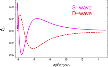
Figure 1: $S$-wave term (solid) and $D$-wave one (dashed) of coupling form factors for $D^{0}\bar{D}^{0*}$ components.

Because the $X(3872)$ is very close to the $D^{0}\bar{D}^{0*}$ threshold, the $1/(z_{X}-E)$ term will greatly enhance the contributions of $f_{ls}\mathcal{M}_{l^{\prime}s^{\prime},ls}$ near the $D^{0}\bar{D}^{0*}$ threshold, and it also leads to extreme suppression of the contributions of the $D$-wave $D\bar{D}^{*}$ components. As an example, $\frac{f_{ls}\mathcal{M}_{l^{\prime}s^{\prime},ls}}{(z_{X}-E)}$ for $S$-wave $D^{0}\bar{D}^{0*}$ or $D^{+}\bar{D}^{-*}$ to $P$-wave $\chi_{c1}\pi^{0}$ is plotted in Fig. 3. Since the flavor wave functions of $\pi^{0}$ is $(\bar{u}u-\bar{d}d)/\sqrt{2}$, the cancellation naturally happens between the neutral charmed states $D^{0}\bar{D}^{0*}$ and the charged $D^{+}\bar{D}^{-*}$ components, which is similar to that of $X(3872)\to J/\psi\rho$ Zhou and Xiao (2018). One could find that the contributions of $D^{0}\bar{D}^{0*}$ and $D^{+}\bar{D}^{-*}$ in the large momentum region will cancel each other and the contribution near the $D^{0}\bar{D}^{0*}$ threshold will be dominant.

In this calculation, the decay rates of $X(3872)$ to $\chi_{cJ}\pi^{0}$ for $J=0,1,2$ turn out to be very small, of the order of $10^{-7}$ GeV, with a ratio $\Gamma_{0}:\Gamma_{1}:\Gamma_{2}=1.5:1.3:1.0$. This ratio is comparable with the effective field theory calculations in Refs.Dubynskiy and Voloshin (2008); Fleming and Mehen (2008). Our calculation also suggests that the magnitude of the decay rates $\chi_{cJ}\pi^{0}$ might not be large even if the $D^{0}\bar{D}^{0*}$ component is dominant. In Refs.Dubynskiy and Voloshin (2008); Fleming and Mehen (2008) a factor determined by the internal dynamics cannot be determined, so they did not present the magnitudes of such decay rates.

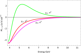
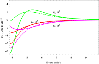
Figure 2: The scattering amplitudes without the phase space factors of $D^{0}\bar{D}^{0*}\to\chi_{c0}\pi^{0}$, $\chi_{c1}\pi^{0}$, $\chi_{c2}\pi^{0}$. The right one shows the prior (solid) and the post (dashed) contributions to the amplitudes. The left one shows the averaged amplitudes.

Figure 3: Comparison of the integrands $\frac{f_{ls}\mathcal{M}_{l^{\prime}s^{\prime},ls}}{(z_{X}-E)}$ for $D^{0}\bar{D}^{0*}\to\chi_{c1}\pi^{0}$ (solid) and $D^{+}\bar{D}^{-*}\to\chi_{c1}\pi^{0}$ (dashed), when $z_{X(3872)}$ is chosen at $3.8716$GeV as an example.

At the same time, we could also calculate the decay rates to $J/\psi\pi^{+}\pi^{-}$ and $J/\psi\pi^{+}\pi^{-}\pi^{0}$ by assuming the final states $\pi^{+}\pi^{-}$ and $\pi^{+}\pi^{-}\pi^{0}$ produced via $\rho$ and $\omega$ resonances, respectively. The interference of neutral and charged $DD^{*}$ components in $X(3872)\to J/\psi\rho$ are destructive, while it is constructive in $X(3872)\to J/\psi\omega$. For simplicity, we describe the $\rho$ and $\omega$ resonances by their Breit-Wigner distribution functions Zhang et al. (2009), and then obtain

$$\Gamma_{J/\psi\pi\pi}=\int_{2m_{\pi}}^{m_{X}-m_{J/\psi}}{\sum_{l,s}}\frac{|F{{}_{l,s}}(X\rightarrow J/\psi\rho)|^{2}\Gamma_{\rho}}{(E-m_{\rho})^{2}+\Gamma_{\rho}^{2}/4}\mathrm{d}E,$$

$$\Gamma_{J/\psi\pi\pi\pi}=\int_{3m_{\pi}}^{m_{X}-m_{J/\psi}}{\sum_{l,s}}\frac{|F{{}_{l,s}}(X\rightarrow J/\psi\omega)|^{2}\Gamma_{\omega}}{(E-m_{\omega})^{2}+\Gamma_{\omega}^{2}/4}\mathrm{d}E,$$

(17)

in which the lower limits of the integration are chosen at the experiment cutoffs as in Refs. Abe et al. (2005); del Amo Sanchez et al. (2010).

The obtained decay width of $J/\psi\pi^{+}\pi^{-}$ is of the order of keV, and the ratio of decay rates to $X(3872)\to\chi_{c0}\pi^{0}$, $\chi_{c1}\pi^{0}$, $\chi_{c2}\pi^{0}$, $J/\psi\pi^{+}\pi^{-}$, and $J/\psi\pi^{+}\pi^{-}\pi^{0}$ is about $1.5:1.3:1.0:16:26$.

This calculation is based on the Barnes-Swanson model and the meson wave functions are approximated by the simple harmonic oscillator wave functions for computing the space overlap factor. This may introduce the “prior-post” discrepancies Barnes and Swanson (1992); Barnes et al. (2001) which are shown in the right graph in Fig. 3. Despite of these discrepancies, the order of magnitudes of the prior and post contributions are similar and we take the average of them as the final amplitudes. Thus we would expect that the absolute magnitude of the decay width is just a rough estimation and only provides an order of magnitude estimate. In this calculation, the decay rate of $X(3872)$ to $\chi_{cJ}\pi^{0}$ is much smaller than to $J/\psi\pi^{+}\pi^{-}$. We think the ratio is reasonable in the mechanism proposed in this paper, because the final $\chi_{cJ}\pi^{0}$ states could only appear in $P$ wave, while the $J/\psi\rho$ states could appear in $S$ wave. Usually, the higher partial waves will be suppressed. Furthermore, the phase space of $\rho\to\pi^{+}\pi^{-}$ will enlarge the decay width of $X(3872)\to J/\psi\pi^{+}\pi^{-}$. In Dong et al. (2009), in the pure molecule picture, an effective field theory calculation gives larger decay widths of $X(3872)$ to $\chi_{cJ}\pi$. However, their branching fraction of ${\mathcal{B}(X(3872)\to\chi_{c1}\pi)}:{\mathcal{B}(X(3872)\to J/\psi\pi^{+}\pi^{-})}$ is about ${(10.2\sim 16.4)}:{(45\sim 54)}$, which also implies a much smaller decay rate to $\chi_{c1}\pi$ than to $J/\psi\pi^{+}\pi^{-}$. In our calculation, the $\chi_{c1}(2P)$ component in the $X(3872)$, which plays an important role in the short range production processes, is expected to contribute little in the long range decay processes and is ignored. As a further check, by using the estimated value of the partial decay width from pure $\chi_{c1}(2P)$ to $\chi_{c1}\pi^{0}$, which is about $0.06$ keV Dubynskiy and Voloshin (2008), and considering the portion of $\chi_{c1}(2P)$ in $X(3872)$ to be about $1/10$, its contribution to the decay width is about $6$ eV, about two orders of magnitude smaller than the contribution from $D\bar{D}^{*}$. Thus, this assumption is still valid.

In addition, the ratio $\frac{\mathcal{B}(X(3872)\to J/\psi\pi^{+}\pi^{-}\pi^{0})}{\mathcal{B}(X(3872)\to J/\psi\pi^{+}\pi^{-})}$ in our calculation is about 1.6, which is comparable with the measured result $1.0\pm 0.4\pm 0.3$ by BelleAbe et al. (2005), $0.8\pm 0.3$ by BABAR del Amo Sanchez et al. (2010) and $1.6^{+0.4}_{-0.3}\pm 0.2$ by BESIII Ablikim et al. (2009). Thus, the isospin breaking effect can be reproduced in this calculation as in Zhou and Xiao (2018).

In summary, by combining the extended Friedrichs scheme and the Barnes-Swanson model, we make a calculation of the decay rates of $X(3872)\to\chi_{c0}\pi^{0}$, $\chi_{c1}\pi^{0}$, $\chi_{c2}\pi^{0}$, $J/\psi\pi^{+}\pi^{-}$, and $J/\psi\pi^{+}\pi^{-}\pi^{0}$ in a unified framework, and find that the relative ratio will be about $1.5:1.3:1.0:16:26$. The decay rate of $X(3872)$ to $\chi_{c1}\pi^{0}$ is one order of magnitude smaller than $X(3872)$ to $J/\psi\pi^{+}\pi^{-}$ in this calculation. Our result is smaller than the central value measured by BESIII Ablikim et al. (2019), but we noticed that the result of BESIII has sizable uncertainties, and more data are needed to increase the statistics and reduce the error bar. In Belle’s experiment, no significant evidence of $X(3872)$ signal was observed in $B^{+}\to\chi_{c1}\pi^{0}K^{+}$ Bhardwaj et al. (2009), though its upper limit of $\frac{\mathcal{B}(X(3872)\to\chi_{c1}\pi^{0})}{\mathcal{B}(X(3872)\to J/\psi\pi^{+}\pi^{-})}$ does not contradict with BESIII’s result. Recently, the Belle II has started to accumulate data with higher statistics and it is expected that more accurate measurements could be obtained in the future.