Cooling of the Cassiopeia A Neutron Star and the
Effect of Diffusive Nuclear Burning

Abstract

The study of how neutron stars cool over time can provide invaluable insights into fundamental physics such as the nuclear equation of state and superconductivity and superfluidity. A critical relation in neutron star cooling is the one between observed surface temperature and interior temperature. This relation is determined by the composition of the neutron star envelope and can be influenced by the process of diffusive nuclear burning (DNB). We calculate models of envelopes that include DNB and find that DNB can lead to a rapidly changing envelope composition which can be relevant for understanding the long-term cooling behavior of neutron stars. We also report on analysis of the latest temperature measurements of the young neutron star in the Cassiopeia A supernova remnant. The 13 Chandra observations over 18 years show that the neutron star’s temperature is decreasing at a rate of 2–3% per decade, and this rapid cooling can be explained by the presence of a proton superconductor and neutron superfluid in the core of the star.

1 INTRODUCTION TO NEUTRON STAR COOLING THEORY

Neutron stars are born in the supernova explosion of a massive star and begin their lives very hot (with thermal energies $kT\gg 1\mbox{ MeV}$ or temperatures $T$ greatly exceeding $10^{10}\mbox{ K}$). They cool rapidly due to neutrino emission and later on by photon emission [1, 2, 3, 4]. Neutrino emission processes depend on physics at densities that exceed nuclear saturation (at baryon density $n_{\rm nuc}\approx 0.16\mbox{ fm${}^{-3}$}$ or mass densities $\rho_{\rm nuc}\approx 2.8\times 10^{14}\mbox{ g cm${}^{-3}$}$). The state of matter is uncertain at these densities, e.g., exotica such as a neutron superfluid and proton superconductor and hyperons, axions, and deconfined quarks could be present [5, 6]. By comparing how neutron stars cool theoretically over time with observations of neutron stars of different ages, one can extract and understand properties of fundamental physics.

Let us consider the basic two equations that govern neutron star cooling. Here for simplicity, we ignore relativistic terms, extra sources of heating, magnetic fields, etc. (see [4], for more details). Then the equations of energy balance and heat flux are

$$\frac{1}{4\pi r^{2}}\frac{\partial L_{r}}{\partial r} = -C\frac{\partial T}{\partial t}-\varepsilon_{\nu}$$ (1)

$$\frac{L_{r}}{4\pi r^{2}} = -K\frac{\partial T}{\partial r},$$ (2)

where $L_{r}$ is luminosity at radius $r$, $C$ is heat capacity, $\varepsilon_{\nu}$ is neutrino emissivity, and $K$ is thermal conductivity. The microphysics inputs that determine how a neutron star cools are $C$, $\epsilon_{\nu}$, and $K$ (see [3, 7, 8]). After a thermal relaxation time of

$$t_{\rm relax}\sim(C/K)R_{\rm crust}^{2}\sim 10-100\mbox{ yr},$$ (3)

where $R_{\rm crust}$ is crust thickness, the temperature gradient becomes small, such that the interior is effectively isothermal, and thermal evolution is determined solely by Equation (1), which can be further simplified by an integration over volume. A final important ingredient of neutron star cooling is the outer layers, or envelope, of the neutron star crust, which prescribes the outer boundary condition for the solution of the cooling equations. Properties of the envelope, such as elemental composition, determine the transition between temperature at the bottom of the envelope (at $\sim 10^{8}-10^{10}\mbox{ g cm${}^{-3}$}$) and temperature at the surface, (i.e. $T_{\rm b}$–$T_{\rm s}$), where surface temperature corresponds to that measured using telescopes such as Chandra and XMM-Newton.

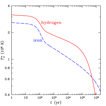
Figure 1: Neutron star (redshifted) surface temperature $T_{\rm s}^{\infty}$ as a function of age. Solid line is for a cooling simulation which uses a hydrogen envelope, while dashed line is one that uses an iron envelope.

Figure 1 illustrates some of the basic features of a cooling neutron star. For instance, there are three stages of neutron star cooling. At early times ($t<t_{\rm relax}$), there is a period of thermal relaxation when $T_{\rm s}\sim\mbox{constant}$. The neutron star core is cooling rapidly because neutrino emission is more effective at high densities. Finite thermal conductivity of lower density regions, such as the crust, delays when this temperature drop is seen at the surface. After this cooling wave from the core reaches the surface at $t\sim t_{\rm relax}$, we see a sharp decline of $T_{\rm s}$. For standard neutrino emission processes (such as the modified Urca reaction, $n+n\rightarrow n+p+e+\bar{\nu}_{\rm e}$, which scales as $\varepsilon_{\nu}\propto T^{8}$), the interior temperature is approximately isothermal and decreases as $T_{\rm b}\propto t^{-1/6}$. Once temperature decreases to the point when neutrino emission becomes less efficient than photon emission (at $t>10^{5}\mbox{ yr}$), the latter becomes the dominant cooling process, and temperature decreases as $T_{\rm b}\propto t^{-1/2}$.

We note here that, when the interior temperature drops below (density-dependent) critical temperatures for proton superconductivity and neutron (${}^{1}S_{0}$ or ${}^{3}P_{2}$) superfluidity, the accompanying phase transition causes two competing effects on cooling. First, superconducting protons and superfluid neutrons no longer participate in standard neutrino emission processes such as the modified Urca reactions, and thus cooling is suppressed (there is also a reduction of heat capacity; [3]). Second, formation and breaking of superfluid or superconducting Cooper pairs lead to a new source of neutrino emission (e.g., $n+n\rightarrow[nn]+\nu+\bar{\nu}$), which enhances cooling [3].

2 ENVELOPE/ATMOSPHERE EVOLUTION AND DIFFUSIVE NUCLEAR BURNING

Figure 1 also shows the dependence of observed surface temperature $T_{\rm s}$ on envelope composition. Since thermal conductivity is higher for light elements ($K\propto 1/Z$), a light element envelope is more transparent to the hot core than a heavy element envelope. An outer layer composed of hydrogen could exist if accretion occurs after neutron star formation. Alternatively, a helium or carbon composition could result from diffusive nuclear burning on the neutron star surface (see next). Finally, a heavy element outer layer would be present if no accretion takes place or if all lighter elements are consumed by nuclear reactions. Each of these compositions gives a different $T_{\rm s}$–$T_{\rm b}$ relation, e.g., $T_{\rm s}/10^{6}\mbox{ K}\sim 2(T_{\rm b}/10^{8}\mbox{ K})^{17/28}$ for hydrogen [9, 10] and $T_{\rm s}/10^{6}\mbox{ K}\sim(T_{\rm b}/10^{8}\mbox{ K})^{11/20}$ for iron [11]. However, these works only consider envelope compositions that do not change with time. Recently, [12] develop $T_{\rm s}$–$T_{\rm b}$ relations for mixed compositions, including H–He, He–C, and C–Fe, and find that diffusion is slow enough to not affect these relations. [13] then use these relations to conduct cooling simulations. However these works do not consider the effects of diffusive nuclear burning (DNB).

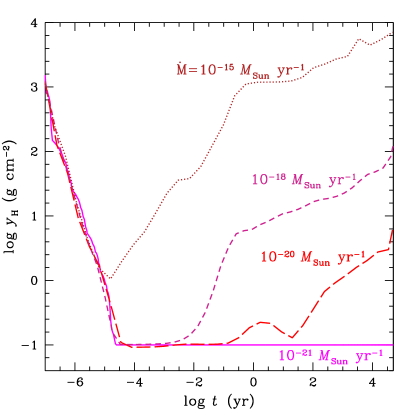
Figure 2: Hydrogen column density $y_{\rm H}$ as a function of time. An initial column of $y_{\rm H}=10^{6}\mbox{ g cm${}^{-2}$}$ and a minimum column of $y_{\rm H}=0.1\mbox{ g cm${}^{-2}$}$ are assumed. Curves are for different mass accretion rates $\dot{M}$.

DNB occurs when temperatures are high enough for nuclear burning to take place in a diffusive tail that extends from the surface into much higher density layers [14, 15, 16, 17]. This light element current can easily deplete surface layers of hydrogen in $<10^{5}\mbox{ yr}$ [17, 18] and helium in $<10^{3}\mbox{ yr}$ [19]. In [20], we account for DNB in H-He and He-C envelopes in calculating new $T_{\rm s}$–$T_{\rm b}$ relations (for H-C, see [21]), which we use in neutron star cooling simulations. Figure 2 shows examples of how the amount of hydrogen at the surface evolves for a H-C envelope, where we allow for an isolated neutron star to accrete from its surrounding environment (e.g., if the environment has a number density of $1\mbox{ cm${}^{-3}$}$ and the neutron star moves at a velocity of $20\mbox{ km s${}^{-1}$}$, then $\dot{M}\sim 10^{-15}\mbox{ $M_{\rm Sun}$\ yr${}^{-1}$}$; see [20], for details). We see that initial hydrogen is consumed within an hour due to high temperatures present soon after neutron star formation. For accretion rates $\dot{M}>10^{-20}\mbox{ $M_{\rm Sun}$\ yr${}^{-1}$}$, the amount of hydrogen builds up again, and there is a sufficient amount to produce at least a hydrogen atmosphere after a few hundred years. Such a neutron star would be observed to have a hydrogen spectrum, while a neutron star accreting at a lower $\dot{M}$ would have a carbon spectrum [22]. Whether we could detect a near real-time change in atmosphere composition is unknown.

3 COOLING OF THE CASSIOPEIA A NEUTRON STAR

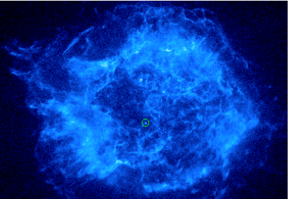
Figure 3: Chandra image (ObsID 14481) of the Cassiopeia A supernova remnant. Circle near the remnant center indicates the neutron star position.

The neutron star in the Cassiopeia A supernova remnant is one of the most important neutron stars because it is the youngest known, at an age of $\approx$340 yr. This estimated age comes from a supernova date of $1681\pm 19$, which is derived from studying the expansion of the supernova remnant [23]. While the remnant has been known about for a long time, the compact object associated with the remnant and near its center (see Figure 3) was only discovered with the launch of Chandra and use of its unparalleled spatial resolution [24]. Although no pulsations are detected from the compact object [25, 26], its identification as a neutron star with a carbon atmosphere can be made from its spectrum [27]. Figure 4 shows neutron star mass $M$ and radius $R$ confidence contours obtained from fitting the star’s spectra (see [20], for details) and assuming a distance of 3.4 kpc [28]. It is important to note that, while the best-fit values are $M=1.65M_{\rm Sun}$ and $R=12.9\mbox{ km}$, these values are not strongly constrained, and the uncertainty region is broad and encompasses many nuclear EOSs. A notable effect of this $M$–$R$ uncertainty is on temperatures derived from spectra (see next), which include fitting for gravitational redshift ($\propto 2GM/Rc^{2}$). As a result, normalization of the absolute value of temperature depends on mass and radius. However relative temperatures do not, and neither does the observed cooling rate. On the other hand, theoretical modeling of the observed cooling rate depends on mass and radius (see, e.g., [29, 30, 31]).

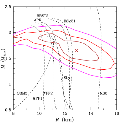
Figure 4: Neutron star mass $M$ and radius $R$. Solid lines are 1$\sigma$, 90%, and 99% confidence contours of $M$–$R$ obtained from fitting Chandra spectra of the Cassiopeia A neutron star. The cross marks the best-fit $M=1.65\,M_{\rm Sun}$ and $R=12.9\mbox{ km}$. Dashed lines indicate $M$–$R$ relation obtained from various theoretical nuclear EOSs, in particular APR [32], BBST2 [33], BSk21 [34], MS0, SQM3, WFF1, WFF2 (see [35], and references therein), and SLy [36].

Following its neutron star identification, successive surface temperature measurements from Chandra spectra show that the neutron star is cooling at a rapid rate [37, 38, 31, 20], likely due to the earlier onset of superconductivity and superfluidity in the neutron star core [29, 30]. Figure 5 shows our latest measurements using 13 Chandra ACIS-S Graded observations over 18 years, which yield ten-year cooling rates of $2.1\pm 0.2\%$ (1$\sigma$) for constant $N_{\rm H}$ and $2.7\pm 0.3\%$ (1$\sigma$) for varying $N_{\rm H}$ [20], where $N_{\rm H}$ measures the column of interstellar material between us and the neutron star that can absorb X-ray photons. In performing our spectral fits, we either fix $N_{\rm H}$ between each observation to be the same value [best-fit $N_{\rm H}=(1.67\pm 0.03)\times 10^{22}\mbox{ cm${}^{-2}$}$] or allow $N_{\rm H}$ to vary between each observation (see Figure 6). Importantly, our cooling rates agree with the latest findings which use a Chandra detector configuration (i.e., ACIS-S subarray) that is optimized for studying the Cassiopeia A neutron star. Using 2 of these observations over 6 years, [39] find no cooling ($1.3\pm 1.0\%$; 90% confidence), and [40] use a third observation that expands the time baseline to 9 years to find ten-year cooling rate upper limits of 2.4% for constant $N_{\rm H}$ and 3.3% for varying $N_{\rm H}$ (both at 3$\sigma$). To illustrate the agreement between both sets of observations, we show temperatures measured by [40] in Figure 5. Because of different values of $M$ and $R$ assumed in [40], as well as uncertainty in instrument cross-calibration, the absolute normalization is somewhat arbitrary. Therefore, we normalized the temperatures from [40] such that temperatures measured in 2015 from observations using the two different Chandra detector configurations taken less than three days apart have the same value.

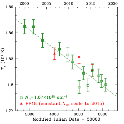
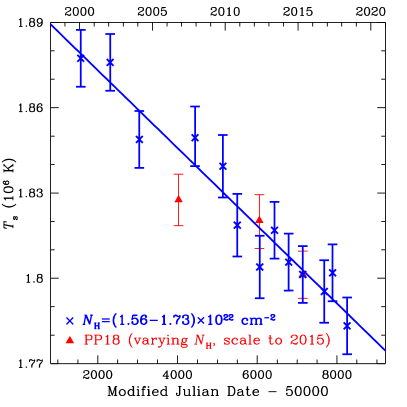
Figure 5: Surface temperature of the neutron star in the Cassiopeia A supernova remnant. Squares and crosses indicate $T_{\rm s}$ measured using Chandra ACIS-S spectra and best-fit neutron star mass $M=1.65\,M_{\rm Sun}$ and radius $R=12.9\mbox{ km}$. Error bars are 1$\sigma$. Lines show a linear fit with a slope of temperature change per decade of 2.1% (left) and 2.7% (right). Left: Interstellar absorption column $N_{\rm H}$ is held constant when fitting 13 observations over 18 years. Right: $N_{\rm H}$ is allowed to vary between each observation. Triangles are 3 values of $T_{\rm s}$ measured using Chandra ACIS-S subarray spectra by PP18 [40]; because of differences in fit parameters $M$, $R$, and $N_{\rm H}$, as well as uncertainty in instrument cross-calibration, these data are normalized by the observations in 2015, which were taken less than 3 days apart.

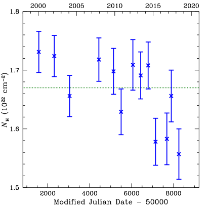
Figure 6: Interstellar X-ray absorption column $N_{\rm H}$ in the direction of the Cassiopeia A neutron star as measured using Chandra spectra. Crosses indicate $N_{\rm H}$ obtained using best-fit neutron star mass $M=1.65\,M_{\rm Sun}$ and radius $R=12.9\mbox{ km}$ and allowing $T_{\rm s}$ to vary, while the horizontal line indicates the constant value ($N_{\rm H}=1.67\times 10^{22}\mbox{ cm${}^{-2}$}$) used in the other spectral fit (see text and Figure 5). Error bars are 1$\sigma$.

4 DISCUSSION

Comparisons between observations of neutron stars and theoretical modeling of neutron star cooling provide us a unique method to understand properties of fundamental physics such as the nuclear EOS and superconductivity and superfluidity. Our recent work [20], summarized here, examines the effect DNB has on the outer layers, spectra, and cooling behavior of isolated neutron stars. Work studying DNB in accreting neutron star systems is in progress [21]. In addition, we use 13 observations made over 18 years by Chandra of the (youngest known) neutron star in the Cassiopeia A supernova remnant to show that this neutron star is cooling at a rapid rate of 2–3% per decade in temperature. Previous works use this cooling rate to infer the density dependence of the critical temperatures for proton superconductivity and neutron superfluidity, which are then compared to theoretically-predicted models [29, 30, 31]. Future work will use the new results to further improve our knowledge of nuclear physics properties (see, e.g., [41, 42]).

Meanwhile, more Chandra observations of Cassiopeia A (and other neutron stars) will be made. An important issue that is the subject of ongoing study is calibration of ACIS detectors onboard Chandra. It is known that a contaminant is building up on these detectors, and this contaminant affects temperature measurements of the Cassiopeia A neutron star [38, 39]. Our recent results [20], as well as those of [40], use the latest models that seek to offset the effects of the contaminant [43, 44]. While the measured variation of $N_{\rm H}$ with time (see Figure 6) could be due to changes in the amount of intervening X-ray absorbing material (see, e.g., [45]), this variation could alternatively be due to incomplete modeling of the contaminant. It would be interesting to determine the nature of this variation, as it affects the cooling rate determination (e.g., 2.1% for constant $N_{\rm H}$ versus 2.7% for varying $N_{\rm H}$). With continued work, future Chandra observations will become more reliable, and neutron star temperature measurements will be more accurate.

5 ACKNOWLEDGMENTS

WCGH is grateful to the organizers of the Xiamen-CUSTIPEN workshop for their support and hospitality and to the referee for their valuable comments. WCGH thanks the staff at the Chandra X-ray Center for their operation and maintenance of Chandra. WCGH acknowledges support through grant ST/R00045X/1 from Science and Technology Facilities Council in the United Kingdom.

References

- Lattimer et al. [1994] J. M. Lattimer, K. A. van Riper, M. Prakash, and M. Prakash, ApJ 425, 802–813 (1994).
- Tsuruta [1998] S. Tsuruta, Phys. Rep. 292, 1–130 (1998).
- Yakovlev, Levenfish, and Shibanov [1999] D. G. Yakovlev, K. P. Levenfish, and Y. A. Shibanov, Physics Uspekhi 42, 737–778 (1999).
- Potekhin, Pons, and Page [2015] A. Y. Potekhin, J. A. Pons, and D. Page, Space Sci. Rev. 191, 239–291 (2015).
- Lattimer [2012] J. M. Lattimer, Annual Review of Nuclear and Particle Science 62, 485–515 (2012).
- Oertel et al. [2017] M. Oertel, M. Hempel, T. Klähn, and S. Typel, Reviews of Modern Physics 89, p. 015007 (2017).
- Gnedin, Yakovlev, and Potekhin [2001] O. Y. Gnedin, D. G. Yakovlev, and A. Y. Potekhin, MNRAS 324, 725–736 (2001).
- Ho, Glampedakis, and Andersson [2012] W. C. G. Ho, K. Glampedakis, and N. Andersson, MNRAS 422, 2632–2641 (2012).
- Potekhin, Chabrier, and Yakovlev [1997] A. Y. Potekhin, G. Chabrier, and D. G. Yakovlev, A&A 323, 415–428 (1997).
- Potekhin et al. [2003] A. Y. Potekhin, D. G. Yakovlev, G. Chabrier, and O. Y. Gnedin, ApJ 594, 404–418 (2003).
- Gudmundsson, Pethick, and Epstein [1983] E. H. Gudmundsson, C. J. Pethick, and R. I. Epstein, ApJ 272, 286–300 (1983).
- Beznogov, Potekhin, and Yakovlev [2016] M. V. Beznogov, A. Y. Potekhin, and D. G. Yakovlev, MNRAS 459, 1569–1579 (2016).
- Beznogov et al. [2016] M. V. Beznogov, M. Fortin, P. Haensel, D. G. Yakovlev, and J. L. Zdunik, MNRAS 463, 1307–1313 (2016).
- Chiu and Salpeter [1964] H.-Y. Chiu and E. E. Salpeter, Physical Review Letters 12, 413–415 (1964).
- Rosen [1968] L. C. Rosen, Ap&SS 1, 372–387 (1968).
- Rosen [1969] L. C. Rosen, Ap&SS 5, 150–170 (1969).
- Chang and Bildsten [2003] P. Chang and L. Bildsten, ApJ 585, 464–474 (2003).
- Chang and Bildsten [2004] P. Chang and L. Bildsten, ApJ 605, 830–839 (2004).
- Chang, Bildsten, and Arras [2010] P. Chang, L. Bildsten, and P. Arras, ApJ 723, 719–728 (2010).
- Wijngaarden et al. [2019] M. J. P. Wijngaarden, W. C. G. Ho, P. Chang, C. O. Heinke, D. Page, M. Beznogov, and D. J. Patnaude, MNRAS 484, 974–988 (2019).
- [21] M. J. P. Wijngaarden, W. C. G. Ho, P. Chang, and et al., in preparation .
- Potekhin [2014] A. Y. Potekhin, Physics Uspekhi 57, 735–770 (2014).
- Fesen et al. [2006] R. A. Fesen, M. C. Hammell, J. Morse, R. A. Chevalier, K. J. Borkowski, M. A. Dopita, C. L. Gerardy, S. S. Lawrence, J. C. Raymond, and S. van den Bergh, ApJ 645, 283–292 (2006).
- Tananbaum [1999] H. Tananbaum, IAU Circ. 7246 (1999).
- Murray et al. [2002] S. S. Murray, S. M. Ransom, M. Juda, U. Hwang, and S. S. Holt, ApJ 566, 1039–1044 (2002).
- Halpern and Gotthelf [2010] J. P. Halpern and E. V. Gotthelf, ApJ 709, 436–446 (2010).
- Ho and Heinke [2009] W. C. G. Ho and C. O. Heinke, Nature 462, 71–73 (2009).
- Reed et al. [1995] J. E. Reed, J. J. Hester, A. C. Fabian, and P. F. Winkler, ApJ 440, p. 706 (1995).
- Page et al. [2011] D. Page, M. Prakash, J. M. Lattimer, and A. W. Steiner, Physical Review Letters 106, p. 081101 (2011).
- Shternin et al. [2011] P. S. Shternin, D. G. Yakovlev, C. O. Heinke, W. C. G. Ho, and D. J. Patnaude, MNRAS 412, L108–L112 (2011).
- Ho et al. [2015] W. C. G. Ho, K. G. Elshamouty, C. O. Heinke, and A. Y. Potekhin, Phys. Rev. C 91, p. 015806 (2015).
- Akmal, Pandharipande, and Ravenhall [1998] A. Akmal, V. R. Pandharipande, and D. G. Ravenhall, Phys. Rev. C 58, 1804–1828 (1998).
- Baldo et al. [2014] M. Baldo, G. F. Burgio, H.-J. Schulze, and G. Taranto, Phys. Rev. C 89, p. 048801 (2014).
- Potekhin et al. [2013] A. Y. Potekhin, A. F. Fantina, N. Chamel, J. M. Pearson, and S. Goriely, A&A 560, p. A48 (2013).
- Lattimer and Prakash [2001] J. M. Lattimer and M. Prakash, ApJ 550, 426–442 (2001).
- Douchin and Haensel [2001] F. Douchin and P. Haensel, A&A 380, 151–167 (2001).
- Heinke and Ho [2010] C. O. Heinke and W. C. G. Ho, ApJ 719, L167–L171 (2010).
- Elshamouty et al. [2013] K. G. Elshamouty, C. O. Heinke, G. R. Sivakoff, W. C. G. Ho, P. S. Shternin, D. G. Yakovlev, D. J. Patnaude, and L. David, ApJ 777, p. 22 (2013).
- Posselt et al. [2013] B. Posselt, G. G. Pavlov, V. Suleimanov, and O. Kargaltsev, ApJ 779, p. 186 (2013).
- Posselt and Pavlov [2018] B. Posselt and G. G. Pavlov, ApJ 864, p. 135 (2018).
- Yakovlev et al. [2011] D. G. Yakovlev, W. C. G. Ho, P. S. Shternin, C. O. Heinke, and A. Y. Potekhin, MNRAS 411, 1977–1988 (2011).
- Shternin and Yakovlev [2015] P. S. Shternin and D. G. Yakovlev, MNRAS 446, 3621–3630 (2015).
- Plucinsky et al. [2016] P. P. Plucinsky, A. Bogdan, G. Germain, and H. L. Marshall, “The evolution of the ACIS contamination layer over the 16-year mission of the Chandra X-ray Observatory,” in Space Telescopes and Instrumentation 2016: Ultraviolet to Gamma Ray, Proc. SPIE, Vol. 9905 (2016) p. 990544.
- Plucinsky et al. [2018] P. P. Plucinsky, A. Bogdan, H. L. Marshall, and N. W. Tice, “The complicated evolution of the ACIS contamination layer over the mission life of the Chandra X-ray Observatory,” in Space Telescopes and Instrumentation 2018: Ultraviolet to Gamma Ray, Society of Photo-Optical Instrumentation Engineers (SPIE) Conference Series, Vol. 10699 (2018) p. 106996B.
- Alp et al. [2018] D. Alp, J. Larsson, C. Fransson, M. Gabler, A. Wongwathanarat, and H.-T. Janka, ApJ 864, p. 175 (2018).