Shared Predictive Cross-Modal Deep Quantization

Abstract

With explosive growth of data volume and ever-increasing diversity of data modalities, cross-modal similarity search, which conducts nearest neighbor search across different modalities, has been attracting increasing interest. This paper presents a deep compact code learning solution for efficient cross-modal similarity search. Many recent studies have proven that quantization based approaches perform generally better than hashing based approaches on single-modal similarity search. In this work, we propose a deep quantization approach, which is among the early attempts of leveraging deep neural networks into quantization based cross-modal similarity search. Our approach, dubbed shared predictive deep quantization (SPDQ), explicitly formulates a shared subspace across different modalities and two private subspaces for individual modalities, representations in the shared subspace and the private subspaces are learned simultaneously by embedding them to a reproducing kernel Hilbert space where the mean embedding of different modality distributions can be explicitly compared. Additionally, in the shared subspace, a quantizer is learned to produce the semantics preserving compact codes with the help of label alignment. Thanks to this novel network architecture in cooperation with supervised quantization training, SPDQ can preserve intra- and inter-modal similarities as much as possible and greatly reduce quantization error. Experiments on two popular benchmarks corroborate that our approach outperforms state-of-the-art methods.

I Introduction

Similarity search is a fundamental subject in numerous computer vision applications, such as image and video retrieval [1, 2, 3, 4, 5, 6, 7, 8, 9, 10, 11, 12, 13, 14, 15], image classification [16], object recognition [17], etc. During the last decade, the amount of heterogeneous multimedia data continues to grow at an astonishing speed, and multimedia data on the Internet usually exist in different media types and come from different data sources, e.g., video-tag pairs from YouTube, image-short text pairs from Facebook, and text-image pairs from news website. When we search a topic, it is expected to retrieve a ranked list containing data in various media types, which can give us a comprehensive description for the query topic. So, efficient cross-modal similarity search becomes increasingly important and has also been found far more challenging.

Actually, cross-modal retrieval has been widely studied in recent years [18, 19, 20, 21, 22, 23, 24, 25, 26]. In contrast to single-modal search scenario, heterogeneous data in cross-modal retrieval usually reside in different feature spaces, and how to exploit and build the correlation between heterogeneous modalities to preserve both intra- and inter-modal data similarities is a crucial issue. In order to eliminate the diversity between different modality features, recent studies are concentrated on mapping heterogeneous data into a common latent subspace so that the learned features in this subspace can be directly compared. However, due to high storage cost and low query efficiency, these methods can not deal with large-scale multi-modal data.

To tackle the efficiency and storage challenges, we study compact coding, a promising solution approaching cross-modal similarity search, especially focusing on a common real-world cross-modal search scenario: image-to-text search. Compact coding methods transform high-dimensional data points to indexable short binary codes, with which similarity search can be executed very efficiently. Most research efforts have been made on cross-modal similarity search with typical solutions including hashing [27, 28, 29, 30, 31, 32, 33, 34, 35, 36, 37, 38, 39, 40, 41, 42, 43, 44] and quantization [39, 45, 46]. Hashing based methods are usually proposed by mapping original heterogeneous high-dimensional data into a common low-dimensional Hamming space and representing the original data by using a set of compact binary codes. Quantization based methods, rather than using binary codes, usually approximate the original data by concatenating or adding a set of learned quantizers. It has been proven that quantization enjoys a more powerful representation ability than hashing, thanks to the more accuracy distance approximation [47, 48, 49, 50]. However, previous cross-modal hashing or quantization methods relying on shallow learning architectures cannot effectively exploit the intrinsic relationships among different modalities.

Recently, deep hashing methods for cross-modal search [51, 21] emerge and yield attractive results on a number of benchmarks. Performance of those methods largely depends on whether those deep hashing models can effectively capture nonlinear correlations between different modalities. To further reduce quantization error, deep quantization method [52] is proposed for cross-modal similarity search, where a deep representation and a quantizer for each modality are jointly learned with an end-to-end architecture. Unfortunately, a common shortcoming of such deep methods, whether hashing or quantization, is that they individually construct two networks for different modalities and then learn their corresponding deep representations, which isolates the relationships among different modalities. Moreover, current quantization strategies do not consider the impact of semantic information (such as labels) on the quality of quantization and similarity preserving.

In this paper, we propose a novel quantization approach for cross-modal similarity search, dubbed Shared Predictive Deep Quantization (SPDQ), aiming at adequately exploiting the intrinsic correlations among multiple modalities and learning compact codes of higher quality in a joint deep network architecture. Specifically, we first adopt deep neural networks to construct a shared subspace and two private subspaces respectively. The private subspaces are used to capture modality specific properties, while the shared subspace is used to capture the representations shared by multiple modalities. Fig.  1 illustrates the difference between traditional common subspace learning methods and the proposed method. Compared with traditional common subspace learning methods [53, 54], by finding a shared subspace that is independent of the private subspaces, our proposed model can capture intrinsic semantic information shared between multi-modal data more efficiently. Actually, representations in shared subspace and private subspaces are learned simultaneously by embedding them to a reproducing kernel Hilbert space where the mean embedding of different modality distributions can be explicitly compared. Moreover, we quantize the representations to produce compact codes in the shared subspace, where label alignment is introduced to enforce semantic similarities. In doing so, data points in the same class are encouraged to have the same representation, therefore greatly reducing intra-class dissimilarity, then both intra- and inter-modal similarities are well preserved. Compared with existing works, main contributions of the proposed SPDQ method are summarized as follows:

• By explicitly learning a shared subspace and two private subspaces, our method can extract the correlated information between different modalities more efficiently.

• Representations from different classes are transformed and aligned using label information, which can greatly reduce the intra-class diversity, and both intra-modal and inter-modal semantic similarities are well preserved.

• By integrating shared and private subspace learning and representation quantization in an end-to-end mechanism, our method can jointly optimize each part and generate more discriminative representations which are suitable for quantization.

• Experimental results on two popular cross-modal datasets show that our approach significantly outperforms state-of-the-arts in terms of search accuracy and search efficiency.

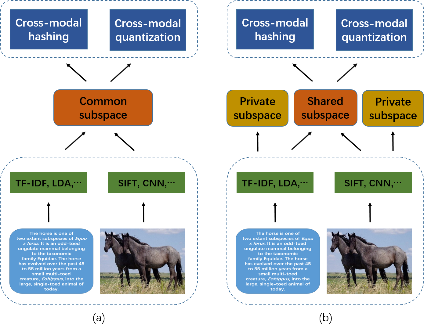
Figure 1: The difference between traditional common subspace learning methods and the proposed SPDQ method: (a) traditional common subspace learning methods, (b) the proposed SPDQ method.

The rest of this paper is organized as follows. We review the relevant literature in Section II. We present our novel deep quantization approach for cross-modal search in Section III. Section V shows the experiments, followed by the concluding remarks in Section VI.

II Related Work

A variety of compact coding approaches for cross-modal similarity search have been developed over the last decade, which include hashing based approaches, quantization based approaches, and more recently deep learning based approaches. We briefly review some work related to our proposed method in this paper.

II-A Cross-modal Hashing

Cross-modal hashing schemes [55] aim at conducting fast similarity search across data from different modalities, which are also similar to the link prediction [56]. In these methods, multi-modal data are usually embedded into a common Hamming space so that hash codes of different modalities can be directly compared using the Hamming distance. Such an embedding can be considered as a hash function acting on input data trying to preserve some underlying similarities. The main challenge in cross-modal hashing lies in how to exploit and build the intrinsic relationships between multiple modalities.

Recently, various cross-modal hashing methods have been proposed. Sensitive hashing (CMSSH) [27] aligns similarities between points in a Hamming space shared across different modalities, where the similarity between a pair of embedded data points is expressed as a superposition of weak classifier. Semantics preserving hashing (SePH) [42] transforms the provided semantic affinities to a probability distribution and approximates it with hash codes in a Hamming space. Considering the learned hash codes as supervised information, SePH learns the hash functions by kernel logistic regression. Co-regularized hashing (CRH) [57] learns hash functions by minimizing an intra-modality loss and an inter-modality loss. Inter-media hashing (IMH) [58] and cross-view hashing (CVH) [33] extend spectral hashing to multi-modal setting. Meanwhile, some endeavors, such as multimodal similarity-preserving hashing [51], sparse hashing [59], composite hashing [38], and collective matrix factorization [60], have been made to exploit similarity relationships to learn hash codes accounting for different modalities.

II-B Cross-modal Quantization

Quantization based methods try to approximate original data using some quantizers. Recently, many kinds of quantization techniques have been proposed including product quantization [61], additive quantization [62] and composite quantization [47]. Product quantization splits the input vector into distinct subvectors which are quantized separately using distinct quantizers. Additive quantization approximates the input vectors using sums of several codewords from different codebooks. Composite quantization is similar to additive quantization and introduces some extra constraints on the inner product between codewords from different codebooks to further improve the query efficiency.

Currently, based on these quantization techniques, some approaches [46, 45, 63] were proposed for cross-modal similarity search. Quantized correlation hashing [46] simultaneously learns hash functions and quantization of hash codes by minimizing the inter-modality similarity disagreement as well as the binary quantization over each modality. Compositional correlation quantization (CCQ) [45] transforms different modalities to an isomorphic latent space, and then quantizes the isomorphic latent features into compact binary codes by learning compositional quantizers. Collaborative quantization [63] jointly learns quantizers for both modalities through aligning the quantized representations for each pair of image and text belonging to a document. Besides, to make the representations in different modalities comparable, collaborative quantization simultaneously learns the common space for both modalities via matrix factorization, and then conducts quantization to enable efficient and effective search via the Euclidean distance in the common space.

II-C Deep Learning Based Cross-modal Methods

Deep learning has revolutionized computer vision [64], machine learning and other related areas, and has also demonstrated its effectiveness in improving accuracy of cross-modal hashing [21, 20] and cross-modal quantization [52]. Deep cross-model hashing (DCMH) [21] exploits pair-wise labels across different modalities to encourage semantic similar data points to have similar hash codes and semantic dissimilar data points to have dissimilar hash codes. Moreover, DCMH integrates feature learning and hash code learning into an unified deep framework. Deep visual-semantic hashing (DVSH) [20] utilizes a convolution neural network for image modality and a recurrent neural network for text modality. It first generates unified compact hash codes by combining information from images and sentences, and then tries to approximate these learned hash codes by training a CNN for image modality and a RNN for text modality. After training, hash codes for instances from different modalities can be directly generated from the corresponding network. Collective deep quantization (CDQ) [52] solves the compact codes learning problem by using a Bayesian learning framework, and learns deep representations and quantizers for all modalities by jointly optimizing these two parts.

Unlike these existing deep cross-modal methods [52, 20, 21], SPDQ is the first attempt to explicitly and jointly model a private subspace for each modality and a shared subspace between different modalities. Additionally, in the process of quantization, we utilize label alignment to greatly improve the quantization quality. Finally, we incorporate these two parts into an end-to-end architecture.

III Formulation

Suppose we have a database $\mathcal{D}$ with two modalities, $\mathcal{D}=\{{(\mathbf{X}_{i},\mathbf{X}_{t}),\mathbf{L}}\}$, where $\mathbf{X}_{i}=\{\mathbf{x}_{i1},\mathbf{x}_{i2},...,\mathbf{x}_{iN}\}$ are data points from image modality, $\mathbf{X}_{t}=\{\mathbf{x}_{t1},\mathbf{x}_{t2},...,\mathbf{x}_{tN}\}$ are data points from text modality, $\mathbf{L}=\{\mathbf{l}_{1},\mathbf{l}_{2},...,\mathbf{l}_{N}\}$ are their corresponding labels with $\mathbf{l}_{n}\in{\{0,1\}}^{K}$, $N$ is the number of data points, and $K$ is the number of classes. $\mathbf{X}_{i}$ can also be formulated as $\mathbf{X}_{i}=\{\mathbf{X}_{i}^{1},\mathbf{X}_{i}^{2},...,\mathbf{X}_{i}^{K}\}$, where $\mathbf{X}_{i}^{k}=\{\mathbf{x}^{k}_{i1},\mathbf{x}^{k}_{i2},...,\mathbf{x}^{k}_{iN_{k}}\}$ are image data points belonging to the $k$-th class, ${N}_{k}$ is the data point number belonging to the $k$-th class. $\mathbf{X}_{t}^{k}$ for text modality is defined similarly.

Given an image (text) query $\mathbf{x}_{iq}$ $\left(\mathbf{x}_{tq}\right)$, the goal of cross-modal similarity search is to retrieve the closest matches in the text (image) database. In this paper, we first exploit convolutional neural networks (CNNs) to learn a shared subspace across different modalities and a private subspace for each modalities. Subsequently, in the shared subspace, we learn common representations by using label alignment and adopt additive quantization [62] to obtain the compact codes. The resulting deep network model is depicted in Fig. 2.

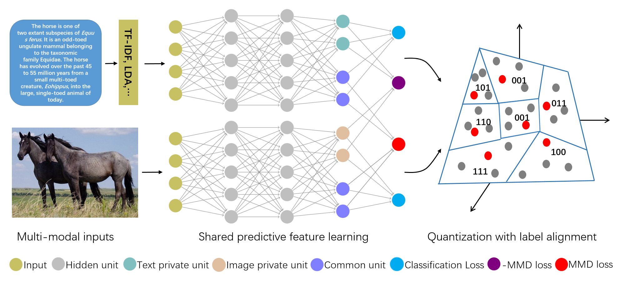
Figure 2: Framework of the proposed method, where text private units and image private units exist in their corresponding modality-specific subspaces and common units exist in the shared subspace.

III-A Shared Predictive Representation Learning

In cross-modal similarity search, representations of two related data points (e.g., an image and an associated text) from different modalities should contain some shared components since they describe the same object. Meanwhile, they should also have private components since they come from different modalities. To achieve accurate search results, the intuitive way is to simply preserve shared components among these representations as much as possible and ignore their private components. However, private components are coupled with shared components in the original representation. According to the idea of subspace decomposition [65] [66] and component analysis [67], explicitly modeling private components can enhance the ability to capture shared components across different modality, thus can achieve more accurate searching. So, in this paper we explicitly model shared components and private components simultaneously.

Concretely, we project the multi-modal data points into a shared subspace and two private subspaces, where the shared components and the private components are captured separately. And we utilize multiple kernel maximum mean discrepancy (MK-MMD) [68] as the distance metric in those subspaces. MK-MMD is a kernel based distance function first proposed for two sample test, and has been successfully used in transfer learning [69] and domain adaptation [70]. In the following, we first give a brief introduction to MK-MMD distance and then elaborate the learning process of the shared subspace and the private subspace.

Let $x$ and $y$ be random variables from distribution $p$ and $q$. The empirical estimate of the distance between $p$ and $q$, as defined by MK-MMD, is

$${d}_{k}^{2}(p,q)={\left\|\mathbb{E}_{x\sim p}[\phi({x})]-\mathbb{E}_{y\sim q}[\phi({y})]\right\|}_{{\mathcal{H}}_{k}}^{2},$$ (1)

where ${\mathcal{H}}_{k}$ is a universal reproducing kernel Hilbert space (RKHS) endowed with a characteristic kernel $k$, $\phi$ is the mapping from original data points to ${\mathcal{H}}_{k}$, and we have $k(x,y)=\left\langle\phi(x),\phi(y)\right\rangle$. For MK-MMD, the characteristic kernel $k$ is a convex combination of $m$ positive semi-definite kernels ${{k}_{u}}$

$$\mathcal{K}:=\left\{k=\mathop{\sum}_{u=1}^{m}{\beta}_{u}{k}_{u}:\mathop{\sum}_{u=1}^{m}{\beta}_{u}=1,{\beta}_{u}\geq 0,\forall u\right\},$$ (2)

where the coefficients $\beta_{u}$ are constrained to guarantee the derived multi-kernel $k$ characteristic. Having a range of kernels is beneficial since the distributions of the features change during learning and different components of the multi-kernel might be responsible at different times, so that we can get a large distance when the distributions are not similar.

In this paper, we exploit MK-MMD as the distance function for learning representations in the shared subspace and the private subspace. As analyzed before, the shared subspace captures common components between different modalities, and the private subspace captures unique components for each modality. So in the shared subspace, representations of data points with the same class from different modalities should be as similar as possible, and in the private subspace, the representations from different modalities reflecting modality-specific information should be as dissimilar as possible. Thus, we can get the following loss function

$$\mathcal{L}_{1} =\mathop{\sum}_{k=1}^{K}\{{\left\|\mathbb{E}[\phi(\mathbf{s}_{i}^{k})]-\mathbb{E}[\phi(\mathbf{s}_{t}^{k})]\right\|}_{{\mathcal{H}}_{k}}^{2}$$ (3)

$$-{\left\|\mathbb{E}[\phi(\mathbf{r}_{i}^{k})]-\mathbb{E}[\phi(\mathbf{r}_{t}^{k})]\right\|}_{{\mathcal{H}}_{k}}^{2}\},$$

where $\mathbf{s}_{i}^{k}$ and $\mathbf{s}_{t}^{k}$ are representations for $\mathbf{x}_{i}^{k}$ and $\mathbf{x}_{t}^{k}$ in the shared subspace, $\mathbf{r}_{i}^{k}$ and $\mathbf{r}_{t}^{k}$ are the corresponding representations in their private subspaces.

To ensure that the modality-specific representations are useful (avoiding trivial solutions) and enhance the discriminative ability of representations in both private subspace and shared subspace, for each modality we concatenate the representations learned from shared subspace and private subspace into a complete representation as $\mathbf{h}_{i}=[\mathbf{s}_{i},\mathbf{r}_{i}]$ and $\mathbf{h}_{t}=[\mathbf{s}_{t},\mathbf{r}_{t}]$. Then, we introduce a classification loss for these complete representations as

$$\mathcal{L}_{2}=\mathcal{L}_{c}(\mathbf{h}_{i},\mathbf{l})+\mathcal{L}_{c}(\mathbf{h}_{t},\mathbf{l}),$$ (4)

where $\mathcal{L}_{c}$ is the sigmoid cross-entropy loss, $\mathbf{l}$ is the corresponding label vector.

Combine (3) and (4), we can formulate the overall objective function for shared predictive representation learning as

$$\mathcal{O}_{l}=\mathcal{L}_{1}+\alpha\mathcal{L}_{2},$$ (5)

where $\alpha$ is the weight to balance these two parts.

For each modality, we design a neural network to learn the shared and private representations as depicted in Fig. 2, which will be elaborated in Section V. By utilizing the designed networks and optimizing the objective function $\mathcal{O}_{l}$, we can explicitly map data points from different modalities into a shared subspace and their modality-specific private subspaces. The networks for the shared subspace learning can be used to predict shared representations for data points from different modalities. Since shared representations contain all the correlated information across different modalities which are crucial for cross-modal retrieval and private components contain only modality-specific information which are inapplicable to cross-modal retrieval, so for the following quantization procedure, we only use the representations in the shared subspace.

III-B Quantization with Label Alignment

If multi-modal data points sharing the same semantic meaning (belong to same categories), it is natural to assume that they share some common structures which are correlated with their labels. Therefore, to preserve the semantic similarity and reduce the intra-class diversity, we assume that representations in shared subspace are composed of category-specific structures which reflect the shared characteristics inside heterogeneous data points, and we use label information to discover and preserve these category-specific structures. The objective function can be defined as

$${\mathcal{L}}_{3}= {\left\|\mathbf{C}_{i}\mathbf{S}_{i}-\mathbf{Z}\mathbf{L}\right\|}^{2}_{F}+{\left\|\mathbf{C}_{t}\mathbf{S}_{t}-\mathbf{ZL}\right\|}^{2}_{F}$$ (6)

$$s.t.\;\mathbf{C}_{i}\mathbf{C}_{i}^{T}=\mathbf{I},\mathbf{C}_{t}\mathbf{C}_{t}^{T}=\mathbf{I},$$

where $\mathbf{S}_{i}=[\mathbf{s}_{i1},\mathbf{s}_{i1},...,\mathbf{s}_{iN}]$ are the representations for image data points in the shared subspace, $\mathbf{S}_{t}=[\mathbf{s}_{t1},\mathbf{s}_{t1},...,\mathbf{s}_{tN}]$ are the representations for text data points in the shared subspace, and $\mathbf{C}_{i}$ and $\mathbf{C}_{t}$ are the transformation matrixes that align $\mathbf{S}_{i}$ and $\mathbf{S}_{t}$ in the label space. In addition, the constraints $\mathbf{C}_{i}\mathbf{C}_{i}^{T}=\mathbf{I},\mathbf{C}_{t}\mathbf{C}_{t}^{T}=\mathbf{I}$ are used to make $\mathbf{C}_{i}$ and $\mathbf{C}_{t}$ be orthogonal projections. We construct an auxiliary matrix $\mathbf{Z}=\left[\mathbf{z}_{1},\mathbf{z}_{2},...\mathbf{z}_{K}\right]$ to reflect the category-specific structures, where $\mathbf{z}_{i}$ is the representation for $i$-th class in the label space. Since all data points sharing the same labels have the same $\mathbf{ZL}$, by optimizing ${\mathcal{L}}_{3}$ we can explicitly reduce the intra-class diversity, and $\mathbf{ZL}$ can be regarded as the surrogate of $\mathbf{C}_{i}\mathbf{S}_{i}$ and $\mathbf{C}_{t}\mathbf{S}_{t}$ in the label space.

Based on the surrogate representations $\mathbf{ZL}$, we adopt additive quantization [62] to learn the final compact codes. Additive quantization aims to approximate representations as the sum of $M$ elements selected from $M$ dictionaries. We can approximate $\mathbf{ZL}$ by minimizing

$${\mathcal{L}}_{4}={\|\mathbf{ZL}-\mathbf{DB}\|}_{F}^{2}.$$ (7)

Here $\mathbf{D}=[\mathbf{D}_{1},\mathbf{D}_{2},...\mathbf{D}_{M}]$ corresponds to $M$ dictionaries, $\mathbf{D}_{m}=[\mathbf{d}_{m1},\mathbf{d}_{m2},...,\mathbf{d}_{mK}]$ corresponds to the $m$-th dictionary with $K$ elements, and $\mathbf{B}=[\mathbf{B}_{1},\mathbf{B}_{2},...,\mathbf{B}_{N}]$ with $\mathbf{B}_{n}=[\mathbf{b}_{n1},\mathbf{b}_{n2},...,\mathbf{b}_{nM}]$ is the indicator matrix, where each $\mathbf{b}_{nm}$ is a 1-of-$K$ binary vector indicating which one (and only one) of the $K$ dictionary elements is selected to approximate the data points.

Combine (6) and (7), we obtain the overall objective function for quantization as

$$\mathcal{O}_{q} =\mathcal{L}_{3}+\beta\mathcal{L}_{4}$$ (8)

$$={\left\|\mathbf{C}_{i}\mathbf{S}_{i}-\mathbf{ZL}\right\|}^{2}_{F}+{\left\|\mathbf{C}_{t}\mathbf{S}_{t}-\mathbf{ZL}\right\|}^{2}_{F}$$

$$+\beta{\left\|\mathbf{ZL}-\mathbf{DB}\right\|}^{2}_{F}$$

$$s.t.\;\mathbf{C}_{i}\mathbf{C}_{i}^{T}=\mathbf{I},\mathbf{C}_{t}\mathbf{C}_{t}^{T}=\mathbf{I},$$

where $\beta$ are weights to balance the two parts.

III-C Overall Objective Function

When merging (5) and (8) together, the overall objective function for learning shared predictive representations and quantizing these representations into compact codes with label alignment can be expressed as

$$\mathcal{O}=\mathcal{O}_{l}+\lambda\mathcal{O}_{q}$$ (9)

$$s.t.\;\mathbf{C}_{i}\mathbf{C}_{i}^{T}=\mathbf{I},\mathbf{C}_{t}\mathbf{C}_{t}^{T}=\mathbf{I},$$

where $\lambda$ is the weight to balance the representation learning and quantization parts. By minimizing (9), we can jointly optimize these two parts which will help to learn more suitable representations for quantization and generate more effectively compact codes.

III-D Search Process

Approximate nearest neighbor (ANN) search based on inner product distance is a powerful technique for quantization methods. Given an image query $\mathbf{x}_{iq}$, we first compute its common representation $\mathbf{s}_{iq}$ using the trained image modality network, and obtain its corresponding representation in the label space denoted as $\mathbf{C}_{i}\mathbf{s}_{iq}$. Similarly to [52], we use Asymmetric Quantizer Distance (AQD) to calculate the distance between the query $\mathbf{x}_{iq}$ and text point $\mathbf{x}_{td}$ in database as

$$AQD(\mathbf{x}_{iq},\mathbf{x}_{td})={\mathbf{C}_{i}\mathbf{s}_{iq}}^{\top}\cdot(\mathop{\sum}_{m=1}^{M}\mathbf{D}_{m}\mathbf{b}_{dm})$$ (10)

where $\mathbf{DB}_{d}=\sum^{M}_{m=1}\mathbf{D}_{m}\mathbf{b}_{dm}$ is the quantized representation for text database point $\mathbf{x}_{ti}$. Given a query, the inner products for all $M$ dictionaries and all $K$ possible values of $\mathbf{b}_{im}$ can be pre-computed and stored in a $M\times K$ lookup table, which is used to compute AQD between the query and all database points. Each AQD calculation entails $M$ table lookups and $M$ additions, and is slightly more costly than Hamming distance.

IV Optimization

We optimize the proposed problem by alternatively solving two sub-problems: updating network parameters with quantization parameters fixed, and updating quantization parameters with the network parameters fixed.

1) Fix quantization parameters $\mathbf{C}_{i}$, $\mathbf{C}_{t}$, $\mathbf{Z}$, $\mathbf{D}$ and $\mathbf{B}$, update network parameters. In this paper, we adopt the unbiased estimate of MK-MMD [68]. Specifically,

$$d_{k}^{2}\left(p,q\right)=\frac{2}{N}\mathop{\sum}_{n=1}^{{N}/{2}}\eta\left(\mathbf{u}_{n}\right),$$ (11)

where, for shared representations, quad-tuple $\mathbf{u}_{n}\triangleq(\mathbf{s}_{i(2n-1)},\mathbf{s}_{i(2n)},\mathbf{s}_{t(2n-1)},\mathbf{s}_{t(2n-1)})$, $N$ is the number of points in a mini-batch, and

$${\eta}(\mathbf{u}_{n}) =k(\mathbf{s}_{i(2n-1)},\mathbf{s}_{i(2n)})-k(\mathbf{s}_{i(2n-1)},\mathbf{s}_{t(2n)})$$ (12)

$$+k(\mathbf{s}_{t(2n-1)},\mathbf{s}_{t(2n)})-k(\mathbf{s}_{t(2n-1)},\mathbf{s}_{i(2n)}).$$

The distance between private representations is similar to the shared representations. When we optimize the network parameters by mini-batch SGD, we only need to consider the gradients of (9) with respect to each data point. Actually we only need to compute the gradients of ${\eta}(\mathbf{u}_{n})$ for the quad-tuple $\mathbf{u}_{n}=(\mathbf{s}_{i(2n-1)},\mathbf{s}_{i(2n)},\mathbf{s}_{t(2n-1)},\mathbf{s}_{t(2n-1)})$. Given kernel $k$ as the convex combination of $m$ Gaussian kernels $\{k_{a}(\mathbf{x}_{i},\mathbf{x}_{j})={e}^{-{\left\|\mathbf{x}_{i}-\mathbf{x}_{j}\right\|}^{2}/{\tau}_{a}}\}$, since:

$$\frac{\partial{k(\mathbf{s}_{i(2n-1)},\mathbf{s}_{i(2n)})}}{\partial\mathbf{s}_{i(2n)}}= -{\sum}_{a=1}^{m}\frac{2{\beta}_{a}}{{\tau}_{a}}{k}_{a}(\mathbf{s}_{i(2n-1)},\mathbf{s}_{i(2n)})$$ (13)

$$\times(\mathbf{s}_{i(2n-1)}-\mathbf{s}_{i(2n)})$$

Combine (1) and (3), the gradient $\frac{\partial{\mathcal{L}_{1}}}{\partial\mathbf{s}_{i\cdot}}$ and $\frac{\partial{\mathcal{L}_{1}}}{\partial\mathbf{r}_{i\cdot}}$ can be readily computed. Since we adopt sigmoid cross-entropy loss for the classification loss in (4), the gradient $\frac{\partial{\mathcal{L}_{2}}}{\partial\mathbf{s}_{in}}$ and $\frac{\partial{\mathcal{L}_{2}}}{\partial\mathbf{r}_{in}}$ can also be readily computed. Then we can get

$$\frac{\partial{\mathcal{O}}}{\partial\mathbf{r}_{in}}=\frac{\partial\mathcal{L}_{1}}{\partial\mathbf{r}_{in}}+\alpha\frac{\partial{\mathcal{L}_{2}}}{\partial\mathbf{r}_{in}},$$ (14)

$$\frac{\partial{\mathcal{O}}}{\partial\mathbf{r}_{tn}}=\frac{\partial\mathcal{L}_{1}}{\partial\mathbf{r}_{tn}}+\alpha\frac{\partial{\mathcal{L}_{2}}}{\partial\mathbf{r}_{tn}}.$$

Fix $\mathbf{C}_{i}$, $\mathbf{C}_{t}$ and $\mathbf{Z}$, we can get

$$\frac{\partial{\mathcal{O}_{q}}}{\partial\mathbf{s}_{in}}=2\mathbf{C_{i}}^{T}(\mathbf{C}_{i}\mathbf{s}_{in}-\mathbf{Zl}_{n}),$$ (15)

$$\frac{\partial{\mathcal{O}_{q}}}{\partial\mathbf{s}_{tn}}=2\mathbf{C_{t}}^{T}(\mathbf{C}_{t}\mathbf{s}_{tn}-\mathbf{Zl}_{n}).$$

Thus we can compute the gradient of the overall objective function $\mathcal{O}$ with regard to $\mathbf{s}_{i}$ and $\mathbf{s}_{t}$ as

$$\frac{\partial{\mathcal{O}}}{\partial\mathbf{s}_{in}}=(\frac{\partial\mathcal{L}_{1}}{\partial\mathbf{s}_{in}}+\alpha\frac{\partial{\mathcal{L}_{2}}}{\partial\mathbf{s}_{in}})+\lambda(\frac{\partial{\mathcal{O}_{q}}}{\partial\mathbf{s}_{in}}),$$ (16)

$$\frac{\partial{\mathcal{O}}}{\partial\mathbf{s}_{tn}}=(\frac{\partial\mathcal{L}_{1}}{\partial\mathbf{s}_{tn}}+\alpha\frac{\partial{\mathcal{L}_{2}}}{\partial\mathbf{s}_{tn}})+\lambda(\frac{\partial{\mathcal{O}_{q}}}{\partial\mathbf{s}_{tn}}).$$

Then using (14) and (16), we can update the parameters of image modality network and text modality network with chain rule.

2) Fix parameters of image modality network and text modality network, $\mathbf{C}_{i}$, $\mathbf{Z}$, when $\mathbf{S}_{i}$ are known, we update the transform matrix $\mathbf{C}_{i}$ by

$${\min}_{\mathbf{C}_{i}}{\left\|\mathbf{C}_{i}\mathbf{S}_{i}-\mathbf{ZL}\right\|}_{F}^{2},$$ (17)

$$s.t.\;\mathbf{C}_{i}\mathbf{C}_{i}^{T}=\mathbf{I}.$$

(17) can be considered as the Orthogonal Procrustes problem and is solved by SVD algorithms. Specifically, we perform SVD as $\mathbf{(ZL)}\mathbf{{S}_{i}}^{T}=\mathbf{U}_{i}\mathbf{Y}_{i}\mathbf{W}^{T}_{i}$, and then we can update $\mathbf{C}_{i}$ by:

$$\mathbf{C}_{i}=\mathbf{U}_{i}\mathbf{W}^{T}_{i}.$$ (18)

3) Fix parameters of image modality network and text modality network, $\mathbf{C}_{t}$ and $\mathbf{Z}$. Similarly to $\mathbf{C}_{i}$, Given $\mathbf{(ZL)}\mathbf{{S}_{t}}^{T}=\mathbf{U}_{t}\mathbf{Y}_{t}\mathbf{W}^{T}_{t}$, We can update the transform matrix $\mathbf{C}_{t}$ by

$$\mathbf{C}_{t}=\mathbf{U}_{t}\mathbf{W}^{T}_{t}.$$ (19)

4) Fix $\mathbf{C}_{i}$, $\mathbf{C}_{t}$, $\mathbf{D}$ and $\mathbf{B}$, let the derivation of $O$ with regard to $\mathbf{Z}$ equals to zero, we can get

$$\mathbf{Z}={[(\mathbf{C}_{i}\mathbf{S}_{i}+\mathbf{C}_{t}\mathbf{S}_{t})+\beta\mathbf{DB}]\mathbf{L}}^{T}{((2+\beta)(\mathbf{L}\mathbf{L}^{T}))}^{-1},$$ (20)

5) Fix $\mathbf{Z}$ and $\mathbf{B}$, and neglect the irrelevant items, we can update the dictionary $\mathbf{D}$ by optimizing

$${\min}_{\mathbf{D}}{\left\|\mathbf{DB-ZL}\right\|}_{F}^{2}.$$ (21)

Eq. (21) is an unconstrained quadratic problem with analytic solution, so we can update $\mathbf{D}$ by

$$D=[\mathbf{ZL}\mathbf{B}^{T}]{[\mathbf{B}\mathbf{B}^{T}]}^{-1}.$$ (22)

6) Fix $\mathbf{D}$ and $\mathbf{Z}$, since each $\mathbf{b}_{n}$ is independent on ${\mathbf{b}_{{n}^{{}^{\prime}}}}\left({{n}^{{}^{\prime}}}\not=n\right)$, the optimization problem for $B$ is decomposed to $N$ subproblems,

$${\min}_{\mathbf{b}_{n}}{\left\|\mathbf{Z}\mathbf{l}_{n}-{\sum}_{m=1}^{M}\mathbf{D}_{m}\mathbf{b}_{nm}\right\|}^{2}$$ (23)

$$s.t.{\left\|\mathbf{b}_{nm}\right\|}_{0}=1,\mathbf{b}_{nm}\in{\{0,1\}}^{K}.$$

This optimization problem in (23) is generally NP-hard. We approximately solve this problem by the Iterated Conditional Modes (ICM) algorithm. Fixing ${\{\mathbf{b}_{n{m}^{{}^{\prime}}}}\}_{{m}^{{}^{\prime}}\not=m}$, $\mathbf{b}_{nm}$ is updated by exhaustively checking all the elements in $\mathbf{D}_{m}$, finding the element such that the objective function is minimized, and setting the corresponding entry of $\mathbf{b}_{nm}$ to be 1 and all the others to be 0. This algorithm is guaranteed to converge and can be terminated if maximum iterations are reached.

Altogether, SPDQ is summarized in Algorithm 1.

Training Stage

Input: Image $\mathbf{X}_{i}$ text $\mathbf{X}_{t}$, semantic labels $\mathbf{L}$, code length $k$, parameters $\alpha$, $\beta$, and $\lambda$.

Output: Parameters for image network and text network, parameters for quantization learning $\mathbf{C}_{i}$, $\mathbf{C}_{t}$, $\mathbf{Z}$, $\mathbf{D}$ and compact codes $\mathbf{B}$.

Procedure:

1. Initialize parameters for image network and text network, initialize $\mathbf{C}_{i}$, $\mathbf{C}_{t}$, $\mathbf{Z}$, $\mathbf{D}$ and $\mathbf{B}$ by random matrices, Mini-batch size $N_{i}=N_{t}=128$.

repeat

      2.1 Randomly sample $N_{i}$ points for $\mathbf{X}_{i}$ and $N_{t}$ points from $\mathbf{X}_{t}$ to construct a mini-batch.

      2.2 Calculate the outputs $\mathbf{s}_{i}$, $\mathbf{s}_{t}$, $\mathbf{r}_{i}$ and $\mathbf{r}_{t}$.

      2.3 Update parameters of image network by (14) and (16).

      2.4 Update parameters of text network by (14) and (16).

      2.5 Update $\mathbf{C}_{i}$ by (18).

      2.6 Update $\mathbf{C}_{t}$ by (19).

      2.7 Update $\mathbf{Z}$ by (20).

      2.8 Update $\mathbf{D}$ by (22).

      2.9 Update $\mathbf{B}$ by the ICM algorithm.

      until Until convergency;

     Testing Stage

      Input: Image query $\mathbf{x}_{i}$ or text query $\mathbf{x}_{t}$, parameters for image network and text network, $\mathbf{C}_{i}$, ${C}_{t}$, $\mathbf{D}$ and $\mathbf{B}$.

      Output: Ranked neighbor list for query

      Procedure:

      1. Calculate the shared representation $\mathbf{s}_{i}$ or $\mathbf{s}_{t}$ by forward the image network or text network.

2. Calculate the distance between query point and the database by (10).

Algorithm 1 Shared predictive Deep quantization

V Experiments

TABLE I: Comparison with baselines with hand-crafted features in terms of MAP. The best accuracy is shown in boldface.

Task	method	FLICKR25K				NUS-WIDE
		16 bits	32 bits	64 bits	128 bits	16 bits	32 bits	64 bits	128 bits
Image Query v.s. Text Database	CMSSH	0.6500	0.6052	0.6106	0.6667	0.7223	0.7354	0.7483	0.7532
	SCM	0.6976	0.6875	0.7089	0.7186	0.6976	0.6854	0.7089	0.7186
	CVH	0.5922	0.5900	0.5913	0.6369	0.6095	0.5917	0.5987	0.6211
	SePH	0.6214	0.6416	0.6433	0.6469	0.6225	0.6296	0.6377	0.6288
	DCMH	0.7576	0.7985	0.8152	0.8369	0.7353	0.7628	0.7805	0.7912
	CDQ	0.9047	0.9094	0.9109	0.8587	0.7917	0.7978	0.8102	0.8214
	Ours	0.9443	0.9476	0.9482	0.8725	0.9276	0.9344	0.9251	0.9299
Text Query v.s. Image Database	CMSSH	0.5014	0.4988	0.5002	0.5015	0.6250	0.6315	0.6445	0.6616
	SCM	0.5693	0.5710	0.5918	0.6028	0.5549	0.5914	0.5991	0.6007
	CVH	0.5352	0.5254	0.5011	0.4705	0.5601	0.5439	0.5160	0.4821
	SePH	0.5506	0.5686	0.5750	0.5837	0.5943	0.5835	0.6119	0.6320
	DCMH	0.7013	0.7288	0.7458	0.7698	0.6898	0.7102	0.7358	0.7557
	CDQ	0.8848	0.8768	0.8841	0.8736	0.8227	0.8184	0.8283	0.8201
	Ours	0.9278	0.9318	0.9313	0.9109	0.8914	0.8983	0.8959	0.8900

TABLE II: Comparison with baselines with CNN features in terms of MAP. The best accuracy is shown in boldface.

Task	method	FLICKR25K				NUS-WIDE
		16 bits	32 bits	64 bits	128 bits	16 bits	32 bits	64 bits	128 bits
Image Query v.s. Text Database	CMSSH	0.6484	0.6484	0.6784	0.5967	0.7074	0.7346	0.7353	0.7450
	SCM	0.7749	0.7868	0.8012	0.8024	0.7885	0.7970	0.8131	0.8209
	CVH	0.7100	0.6776	0.6438	0.6154	0.7157	0.6988	0.6573	0.5993
	SePH	0.7991	0.8199	0.8435	0.8480	0.7893	0.8052	0.8198	0.8333
	DCMH	0.7576	0.7985	0.8152	0.8369	0.7353	0.7628	0.7805	0.7912
	CDQ	0.9047	0.9094	0.9109	0.8587	0.7917	0.7978	0.8102	0.8214
	Ours	0.9443	0.9476	0.9482	0.8725	0.9276	0.9344	0.9251	0.9299
Text Query v.s. Image Database	CMSSH	0.5890	0.5752	0.5795	0.5714	0.6556	0.6749	0.7065	0.7230
	SCM	0.6624	0.6663	0.6837	0.6880	0.6922	0.6854	0.7140	0.7244
	CVH	0.7220	0.6522	0.5972	0.5784	0.7085	0.7383	0.7553	0.7475
	SePH	0.7454	0.7421	0.7614	0.7893	0.6947	0.7062	0.7235	0.7251
	DCMH	0.7013	0.7288	0.7458	0.7698	0.6898	0.7102	0.7358	0.7557
	CDQ	0.8848	0.8768	0.8841	0.8736	0.8227	0.8184	0.8283	0.8201
	Ours	0.9278	0.9318	0.9313	0.9109	0.8914	0.8983	0.8959	0.8900

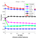
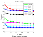
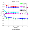
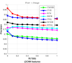
Figure 3: Precision values at various numbers of top retrieved data points on FLICKR25K with code length 16.

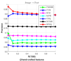
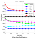
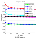
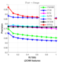
Figure 4: Precision values at various numbers of top retrieved data points on FLICKR25K with code length 32.

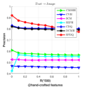
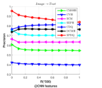
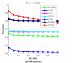
Figure 5: Precision values at various numbers of top retrieved data points on NUS-WIDE with code length 16.

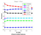
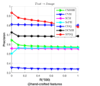
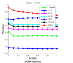
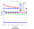
Figure 6: Precision values at various numbers of top retrieved data points on NUS-WIDE with code length 32.

V-A Setup

Datasets. We evaluate our method on two popular benchmark datasets, FLICKR25K and NUS-WIDE. All the data sets have two modalities, i.e. image and text. Some statistics of them are introduced below.

FLICKR25K originally contains 25,000 images collected from the Flickr website. Each image associates with several textual tags and is manually annotated with at least one of 24 provided unique labels. In our experiment, we only keep those textual tags appearing at least 20 times and remove image-tag pairs without manually annotated labels. Then we get 20,015 image-tag pairs for experiment. The text for each point is represented as a 1,386-dimensional bag-of-words vector. The hand-crafted feature for each image is represented by a 512-dimensional GIST feature vector.

NUS-WIDE contains 269,648 images with associated tags, where each pair is annotated with multiple labels among 81 concepts. Following prior works [60, 57], we use the subset of 186,577 image-text pairs that belong to 10 most popular concepts. The text for each point is represented as a 1,000-dimensional bag-of-words vector. The hand-crafted feature for each image is a 500-dimensional bag-of-visual words (BOVW) vector.

For our proposed approach and deep learning based compared methods, we directly use raw pixels as the image modality inputs. For traditional shallow methods, besides the shallow features introduced above, we extract 4096-dimensional feature vectors from the last fully connected layer by using AlexNet architecture [71] pre-trained on ImageNet dataset. So, we compared our method with traditional shallow methods with hand-crafted features as well as deep features. For FLICKR25K, we randomly select 2,000 instances as a test set, the rest are used as a validation set, from which we randomly select 10,000 instances as a training set. For NUS-WIDE, following [72], we randomly select 1866 of the dataset as a test set, the rest are used as a validation set, from which we randomly select 10,000 instances as a training set.

Evaluation. Two evaluation criteria are adopted to evaluate the performance of the proposed method, namely mean of average precision (MAP) and topN-precision. These two criteria are based on Hamming ranking which ranks all the data points based on the Hamming distances to the query.

MAP is one of the most widely-used criteria to evaluate retrieval accuracy. Given a query and a list of $R$ ranked retrieval results, the average precision (AP) for this query is defined as

$$AP=\frac{1}{N}\mathop{\sum}_{r=1}^{R}P(r)\delta{(r)},$$ (24)

where $N$ in the number of ground-truth relevant instances in the database for the query, and $P(r)$ presents the precision for the top $r$ retrieved instances. $\delta{(r)}=1$ when the $r$-th retrieval instance is relevant to the query, otherwise $\delta{(r)}=0$. MAP is defined as the average of APs for all the queries. $R$ is set to 50 in our experiments. The ground-truth relevant instances for a query are defined as those sharing at least one label with it. TopN-precision shows the precision at different numbers of retrieved instances.

Compared methods. We compare the proposed approach with various state-of-the-art cross-modal similarity search methods. Specifically, we take six supervised methods: SCM[73], SePH[42], CMSSH [27], CVH [33], DCMH [21], CDQ [52], as baselines, where DCMH is deep hashing cross-modal method, and CDQ is deep quantization cross-modal method. Source codes of all baseline methods are kindly provided by the authors. Since, SePH is a kernel-based method, we use RBF kernel and take 500 randomly selected points as kernel bases by following its authors’ suggestion. The parameters for all the above methods are set according to the original papers.

Implementation details. As shown in Fig. 2, the hybrid deep architecture constitutes an image network and a text network. For the image network, we adopt the AlexNet architecture [71], and replace the last fully connected layer by a shared layer and a private layer. We set the shared layer with 256 units and the private layer with 48 units and use the hyperbolic tangent (tanh) function as the activation functions. Parameters for the shared layers and the private layers are learned from scratch, and all parameters for the preceding layers are fine-tuned from the model pre-trained on ImageNet dataset. For text modality, we use a three-layer MLP, where the first and the second fully connected layers both have 4,096 units, and the last fully connected layer is replaced by a shared layer and a private layer, which have the same number units as in the image network. All of the parameters for the text network are learned from scratch. We employ the standard stochastic gradient descent algorithm for optimization with 0.9 momentum, fix min-batch size to 128, and the learning rate is chosen from $10^{-6}$ to $10^{-1}$ with a validation set. All experiments are run for five times, and the average performance is reported. Similarly to [45], we set the number of elements in each dictionary as $K=256$, so for each data point, the binary code length $M=C{\log}_{2}D=8C$ bits. We can set $C={M}\verb|/|{8}$ when $M$ is known.

V-B Results and Discussions

For all the datasets, we first present MAP values of all the methods for various code lengths to providing a global evaluation. Then we report the topN-precision curves with code length 16 and 32 to make a comprehensive contrastive study.

The MAP results for SPDQ, DCMH, CDQ and other baselines with hand-crafted features on FLICKR25K and NUS-WIDE datasets are reported in Table I. Here, “$I\to T$” represents the case where the query is image and the database is text, and “$T\to I$” represents the case where the queries are texts and the database are images. We can find that DCMH, CDQ and SPDQ which are both deep learning based methods outperform all the other shallow baselines with hand-crafted features by a large margin. There may be two possible reasons. The first is that since all these deep learning based methods are build upon some existing deep architectures, and the features extracted from these deep architectures have shown to achieve far superior performance than traditional hand-crafted features in various tasks, so the better performance obtained by these deep learning based methods may be from superior features. The second reason may be that by designing more suitable loss functions or architectures and jointly optimizing the feature extraction and hash code learning, these methods can better capture the semantic information than other methods.

To further verify the effectiveness of our SPDQ, for image modality, we extract CNN features from AlexNet pre-trained on ImageNet dataset, which is the same as the initial CNN for image modality in SPDQ. Then, all the shallow baselines are trained based on these CNN features. Table II shows the MAP values for all the methods with code length varying from 16-bit to 128-bit. Compared Table I and Table II, we can see that most of the shallow methods obtain an increase in MAP values in all code lengths, which demonstrates that features extracted from existing deep architectures can usually preserve more semantic information and achieve better performance than traditional hand-crafted features. Despite that, SPDQ and CDQ usually outperform other baseline methods, and DCMH achieves comparable results in many cases. One of the reasons may be that by incorporating feature learning and hash code learning in an end-to-end architecture, these methods can jointly optimize these two parts thus causing better results. Besides, as shown in Table II, the proposed SPDQ outperforms all shallow baselines using CNN features with different code lengths on all retrieval tasks, and also outperforms DCMH, the state-of-the-art deep cross-modal hashing method, as well as CDQ the state-of-the-art deep cross-modal quantization method, which well demonstrates the superiority of the proposed method.

TopN-precision curves on FLICKR25K and NUS-WIDE are showed in Fig. 3, Fig. 4, Fig. 5, and Fig. 6, where Fig. 3 and Fig. 4 show the result with code length 16, and Fig. 5 and Fig. 6 show the results with code length 32. For each figure, the first two sub-figures are based on hand-crafted features and the last two sub-figures are based on CNN features for shallow baseline methods. It can be seen that the proposed approach outperforms all the baseline methods for both hand-crafted features and CNN features. Our SPDQ can also achieve the best performance on other cases with different code lengths, such as 64 and 128. Those results are omitted due to space limitation. The result of TopN-precision curves are consistent with the mAP evaluation. In retrieval system, since the users always focus on the front returned results, the relevance of the top returned instances with the query is usually more important. From the topN-precision curves, we can find that the proposed approach usually outperforms other methods by a large margin when the number of the returned instances are relatively small.

V-C Effect of Training Size

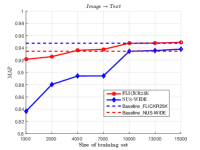
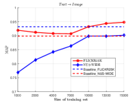
Figure 7: MAP versus the size of training set.

In this subsection, we analyze the effects of training set size on the performance of SPDQ on FLICKR25K and NUS-WIDE dataset. Specifically, we fix the hash code length at 32 bits, and vary the training set size from 1,000 to 15,000. Then we measure MAP values of SPDQ and show the results in Fig. 7. MAP values with training set size 10,000 are chosen as the baseline values. It is easy to see that SPDQ usually obtain better retrieval performance with larger training set size. The increasing trend is particularly apparent for NUS-WIDE dataset, which may be because that NUS-WIDE dataset contains far more data points than FLICKR25K and have more diversities, thus needs more training data to capture the relationships of the whole dataset.

V-D Parameter Sensitivity Analysis

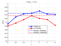
Figure 8: MAP versus parameter $\alpha$.

In this part, we evaluate the effects of the parameters of SPDQ. MAP values on the query dataset are reported to study the performance variation with respect to different parameter values. In this experiments, hash code length is fixed as 32 bits, and we conduct the analysis for one parameter by varying its value while fixing the other parameters. The MAP values of SPDQ with $\alpha=1$, $\beta=1$, $\lambda=0.01$ are selected as the baseline values.

The parameter $\alpha$ controls the importance of the classification loss. We vary its value from $0.1$ to $10$. As shown in Fig. 8, it can be found that the MAP values on both tasks increase with $\alpha$ increasing from $0.1$ to $1$, which may prove that adding the classification loss can enhance the discriminative ability of the learned features. But when $\alpha$ is too large, the classification loss will dominate the training process and effect the quantization learning. In our experiments, we choose $\alpha$ as $1$.

The parameter $\beta$ leverages the importance of label alignment and quantization. When $\beta$ is large, quantization error will be small and approximate error in label alignment part will be large, and vice versa. To measure the concrete influence of $\beta$, we fix other parameters and report the MAP values by varying the value of $\beta$ between the range of $[0.1,10]$. As shown in Fig. 9, we can observe that the performance usually is improved with the increase of $\beta$ from $0.1$ to $1$. When $\beta$ is larger than $1$, the performance of SPDQ will decrease with the increase of $\beta$. So, in our experiments, we set $\beta$ to $1$.

Figure 9: MAP versus parameter $\beta$.

The parameter $\gamma$ reflects the importance of the shared feature learning part and the label alignment quantization part. A proper value of $\gamma$ will enable SPDQ to learn shared features more suitable for quantization. To decide the optimal value of $\gamma$, we fix the hash code length as 32, and calculate the MAP values on FLICKR25K and NUS-WIDE dataset by varying $\gamma$ from $10^{-5}$ to $1$. The results are reported in Fig. 10. It can be observed that the performance on both datasets are relatively stable when $\gamma$ is small than $0.005$, and will decrease apparently when $\gamma$ is larger than $0.005$. Actually, we can select $\gamma$ from the range of $[10^{-5},5\times 10^{-3}]$.

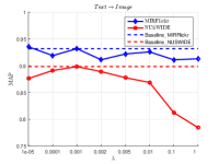
Figure 10: MAP versus parameter $\gamma$.

VI Conclusions

In this paper, we proposed a novel quantization approach, namely shared predictive deep quantization (SPDQ), for efficient cross-modal similarity search. The superiority of the proposed approach lies in: 1) firstly exploiting a deep neural network to construct the shared subspace across different modalities and the private subspace for each modality, in which the correlations between multiple modalities can be well discovered and the specific characteristics of each modality can also be maintained; 2) introducing label alignment to the quantization training procedure, thus preserving the semantic similarities of image-text pairs and greatly improving the search accuracy. The experimental results on two benchmark multi-modal datasets demonstrate that the proposed approach surpasses the existing methods.

References

- [1] W. Liu, J. Wang, R. Ji, Y. Jiang, and S.-F. Chang, “Supervised hashing with kernels,” in CVPR, 2012, pp. 2074–2081.
- [2] Q. Liu, G. Liu, L. Li, X.-T. Yuan, M. Wang, and W. Liu, “Reversed spectral hashing,” IEEE Transactions on Neural Networks and Learning Systems, 2017.
- [3] J. Gui, T. Liu, Z. Sun, D. Tao, and T. Tan, “Fast supervised discrete hashing,” IEEE Transactions on Pattern Analysis and Machine Intelligence, 2017.
- [4] J. Wang, W. Liu, S. Kumar, and S.-F. Chang, “Learning to hash for indexing big data a survey,” Proceedings of the IEEE, vol. 104, no. 1, pp. 34–57, 2016.
- [5] C. Deng, R. Ji, W. Liu, D. Tao, and X. Gao, “Visual reranking through weakly supervised multi-graph learning,” in ICCV, 2013, pp. 2600–2607.
- [6] S. Chang, G.-J. Qi, C. C. Aggarwal, J. Zhou, M. Wang, and T. S. Huang, “Factorized similarity learning in networks,” in Data Mining (ICDM), 2014 IEEE International Conference on. IEEE, 2014, pp. 60–69.
- [7] W. Liu, J. Wang, S. Kumar, and S.-F. Chang, “Hashing with graphs,” in Proceedings of the 28th international conference on machine learning (ICML-11). Citeseer, 2011, pp. 1–8.
- [8] L. Liu and L. Shao, “Sequential compact code learning for unsupervised image hashing,” IEEE Transactions on Neural Networks and Learning Systems, vol. 27, no. 12, pp. 2526–2536, 2016.
- [9] J. Gui, T. Liu, Z. Sun, D. Tao, and T. Tan, “Supervised discrete hashing with relaxation,” IEEE Transactions on Neural Networks and Learning Systems, 2016.
- [10] F. Zhao, Y. Huang, L. Wang, and T. Tan, “Deep semantic ranking based hashing for multi-label image retrieval,” in Proceedings of the IEEE Conference on Computer Vision and Pattern Recognition, 2015, pp. 1556–1564.
- [11] K. Ding, C. Huo, B. Fan, S. Xiang, and C. Pan, “In defense of locality-sensitive hashing,” IEEE Transactions on Neural Networks and Learning Systems, 2016.
- [12] Z. Yu, H.-S. Wong, J. You, and G. Han, “Visual query processing for efficient image retrieval using a som-based filter-refinement scheme,” Information Sciences, vol. 203, pp. 83–101, 2012.
- [13] G.-J. Qi, C. Aggarwal, Q. Tian, H. Ji, and T. Huang, “Exploring context and content links in social media: A latent space method,” IEEE Transactions on Pattern Analysis and Machine Intelligence, vol. 34, no. 5, pp. 850–862, 2012.
- [14] S. You, C. Xu, C. Xu, and D. Tao, “Learning from multiple teacher networks,” in Proceedings of the 23rd ACM SIGKDD International Conference on Knowledge Discovery and Data Mining. ACM, 2017, pp. 1285–1294.
- [15] X. Liu, C. Deng, Y. Mu, and Z. Li, “Boosting complementary hash tables for fast nearest neighbor search.” in AAAI, 2017, pp. 4183–4189.
- [16] B. Kulis and K. Grauman, “Kernelized locality-sensitive hashing for scalable image search,” in ICCV, 2009, pp. 2130–2137.
- [17] J. R. R. Uijlings, K. E. A. Van De Sande, T. Gevers, and A. W. M. Smeulders, “Selective search for object recognition,” International Journal of computer vision, vol. 104, no. 2, pp. 154–171, 2013.
- [18] J. Zhou, G. Ding, and Y. Guo, “Latent semantic sparse hashing for cross-modal similarity search,” in Proceedings of the 37th international ACM SIGIR conference on Research & development in information retrieval, 2014, pp. 415–424.
- [19] C. Deng, X. Tang, J. Yan, W. Liu, and X. Gao, “Discriminative dictionary learning with common label alignment for cross-modal retrieval,” IEEE Transactions on Multimedia, vol. 18, no. 2, pp. 208–218, 2016.
- [20] Y. Cao, M. Long, J. Wang, Q. Yang, and P. S. Yu, “Deep visual-semantic hashing for cross-modal retrieval,” in SIGKDD, 2016, pp. 1445–1454.
- [21] Q. Jiang and W. Li, “Deep cross-modal hashing,” arXiv preprint arXiv:1602.02255, 2016.
- [22] X. Liu, L. Huang, C. Deng, J. Lu, and B. Lang, “Multi-view complementary hash tables for nearest neighbor search,” in Proceedings of the IEEE International Conference on Computer Vision, 2015, pp. 1107–1115.
- [23] X. Liu, L. Huang, C. Deng, B. Lang, and D. Tao, “Query-adaptive hash code ranking for large-scale multi-view visual search,” IEEE Transactions on Image Processing, vol. 25, no. 10, pp. 4514–4524, 2016.
- [24] Y. Luo, D. Tao, C. Xu, C. Xu, H. Liu, and Y. Wen, “Multiview vector-valued manifold regularization for multilabel image classification,” IEEE Transactions on Neural Networks and Learning Systems, vol. 24, no. 5, pp. 709–722, 2013.
- [25] L. Duan, D. Xu, and I. W.-H. Tsang, “Domain adaptation from multiple sources: A domain-dependent regularization approach,” IEEE Transactions on Neural Networks and Learning Systems, vol. 23, no. 3, pp. 504–518, 2012.
- [26] G.-J. Qi, C. C. Aggarwal, and T. S. Huang, “On clustering heterogeneous social media objects with outlier links,” in Proceedings of the fifth ACM international conference on Web search and data mining. ACM, 2012, pp. 553–562.
- [27] M. M. Bronstein, A. M. Bronstein, F. Michel, and N. Paragios, “Data fusion through cross-modality metric learning using similarity-sensitive hashing,” in CVPR, 2010, pp. 3594–3601.
- [28] W. Liu, J. Wang, Y. Mu, S. Kumar, and S.-F. Chang, “Compact hyperplane hashing with bilinear functions,” arXiv preprint arXiv:1206.4618, 2012.
- [29] C. Deng, H. Deng, X. Liu, and Y. Yuan, “Adaptive multi-bit quantization for hashing,” Neurocomputing, vol. 151, pp. 319–326, 2015.
- [30] C. Deng, X. Liu, Y. Mu, and J. Li, “Large-scale multi-task image labeling with adaptive relevance discovery and feature hashing,” Signal Processing, vol. 112, pp. 137–145, 2015.
- [31] T. Ji, X. Liu, C. Deng, L. Huang, and B. Lang, “Query-adaptive hash code ranking for fast nearest neighbor search,” in Proceedings of the 22nd ACM international conference on Multimedia. ACM, 2014, pp. 1005–1008.
- [32] J. Liu, S. Zhang, W. Liu, C. Deng, Y. Zheng, and D. N. Metaxas, “Scalable mammogram retrieval using composite anchor graph hashing with iterative quantization,” IEEE Transactions on Circuits and Systems for Video Technology, vol. 27, no. 11, pp. 2450–2460, 2017.
- [33] S. Kumar and R. Udupa, “Learning hash functions for cross-view similarity search,” in IJCAI, 2011, pp. 1360–1365.
- [34] X. Liu, C. Deng, B. Lang, D. Tao, and X. Li, “Query-adaptive reciprocal hash tables for nearest neighbor search,” IEEE Transactions on Image Processing, vol. 25, no. 2, pp. 907–919, 2016.
- [35] Y. Liu, Z. Chen, C. Deng, and X. Gao, “Joint coupled-hashing representation for cross-modal retrieval,” in Proceedings of the International Conference on Internet Multimedia Computing and Service. ACM, 2016, pp. 35–38.
- [36] X. Liu, X. Fan, C. Deng, Z. Li, H. Su, and D. Tao, “Multilinear hyperplane hashing,” in Proceedings of the IEEE Conference on Computer Vision and Pattern Recognition, 2016, pp. 5119–5127.
- [37] E. Yang, C. Deng, W. Liu, X. Liu, D. Tao, and X. Gao, “Pairwise relationship guided deep hashing for cross-modal retrieval.” in AAAI, 2017.
- [38] D. Zhang, F. Wang, and L. Si, “Composite hashing with multiple information sources,” in SIGIR, 2011, pp. 225–234.
- [39] G. Irie, H. Arai, and Y. Taniguchi, “Alternating co-quantization for cross-modal hashing,” in ICCV, 2015, pp. 1886–1894.
- [40] W. Liu, C. Mu, S. Kumar, and S.-F. Chang, “Discrete graph hashing,” in Advances in Neural Information Processing Systems, 2014, pp. 3419–3427.
- [41] X. Liu, J. He, C. Deng, and B. Lang, “Collaborative hashing,” in Proceedings of the IEEE Conference on Computer Vision and Pattern Recognition, 2014, pp. 2139–2146.
- [42] Z. Lin, G. Ding, M. Hu, and J. Wang, “Semantics-preserving hashing for cross-view retrieval,” in CVPR, 2015, pp. 3864–3872.
- [43] M. Yu, L. Liu, and L. Shao, “Binary set embedding for cross-modal retrieval,” IEEE Transactions on Neural Networks and Learning Systems, 2016.
- [44] K. Li, G.-J. Qi, J. Ye, and K. A. Hua, “Linear subspace ranking hashing for cross-modal retrieval,” IEEE transactions on pattern analysis and machine intelligence, vol. 39, no. 9, pp. 1825–1838, 2017.
- [45] M. Long, J. Cao, Y.and Wang, and P. S. Yu, “Composite correlation quantization for efficient multimodal retrieval,” in SIGIR, 2016, pp. 579–588.
- [46] B. Wu, Q. Yang, W. Zheng, Y. Wang, and J. Wang, “Quantized correlation hashing for fast cross-modal search,” in IJCAI, 2015, pp. 3946–3952.
- [47] T. Zhang, C. Du, and J. Wang, “Composite quantization for approximate nearest neighbor search.” in ICML, no. 2, 2014, pp. 838–846.
- [48] Z. Yu and H.-S. Wong, “Quantization-based clustering algorithm,” Pattern Recognition, vol. 43, no. 8, pp. 2698–2711, 2010.
- [49] K. He, F. Wen, and J. Sun, “K-means hashing: An affinity-preserving quantization method for learning binary compact codes,” in CVPR, 2013, pp. 2938–2945.
- [50] T. Zhang, G.-J. Qi, J. Tang, and J. Wang, “Sparse composite quantization,” in Proceedings of the IEEE Conference on Computer Vision and Pattern Recognition, 2015, pp. 4548–4556.
- [51] J. Masci, M. M. Bronstein, A. M. Bronstein, and J. Schmidhuber, “Multimodal similarity-preserving hashing,” IEEE Trans. on pattern analysis and machine intelligence, vol. 36, no. 4, pp. 824–830, 2014.
- [52] Y. Cao, M. Long, J. Wang, and S. Liu, “Collective deep quantization for efficient cross-modal retrieval,” in AAAI, 2017.
- [53] Z. Yu, L. Li, J. Liu, and G. Han, “Hybrid adaptive classifier ensemble,” IEEE transactions on cybernetics, vol. 45, no. 2, pp. 177–190, 2015.
- [54] Z. Yu, H. Chen, J. Liu, J. You, H. Leung, and G. Han, “Hybrid -nearest neighbor classifier,” IEEE transactions on cybernetics, vol. 46, no. 6, pp. 1263–1275, 2016.
- [55] H. Peng, C. Deng, L. An, X. Gao, and D. Tao, “Learning to multimodal hash for robust video copy detection,” in Image Processing (ICIP), 2013 20th IEEE International Conference on. IEEE, 2013, pp. 4482–4486.
- [56] G.-J. Qi, C. C. Aggarwal, and T. Huang, “Link prediction across networks by biased cross-network sampling,” in Data Engineering (ICDE), 2013 IEEE 29th International Conference on. IEEE, 2013, pp. 793–804.
- [57] Y. Zhen and D. Yeung, “Co-regularized hashing for multimodal data,” in NIPS, 2012, pp. 1376–1384.
- [58] J. Song, Y. Yang, Y. Yang, Z. Huang, and H. Shen, “Inter-media hashing for large-scale retrieval from heterogeneous data sources,” in SIGMOD, 2013, pp. 785–796.
- [59] F. Wu, Z. Yu, Y. Yang, S. Tang, Y. Zhang, and Y. Zhuang, “Sparse multi-modal hashing,” IEEE Trans. on Multimedia, vol. 16, no. 2, pp. 427–439, 2014.
- [60] G. Ding, Y. Guo, and J. Zhou, “Collective matrix factorization hashing for multimodal data,” in Proceedings of the IEEE Conference on Computer Vision and Pattern Recognition, 2014, pp. 2075–2082.
- [61] H. Jegou, M. Douze, and C. Schmid, “Product quantization for nearest neighbor search,” IEEE transactions on pattern analysis and machine intelligence, vol. 33, no. 1, pp. 117–128, 2011.
- [62] A. Babenko and V. Lempitsky, “Additive quantization for extreme vector compression,” in Proceedings of the IEEE Conference on Computer Vision and Pattern Recognition, 2014, pp. 931–938.
- [63] T. Zhang and J. Wang, “Collaborative quantization for cross-modal similarity search,” in CVPR, 2016, pp. 2036–2045.
- [64] G.-J. Qi, “Loss-sensitive generative adversarial networks on lipschitz densities,” arXiv preprint arXiv:1701.06264, 2017.
- [65] K. Bousmalis, G. Trigeorgis, N. Silberman, D. Krishnan, and D. Erhan, “Domain separation networks,” in NIPS, 2016, pp. 343–351.
- [66] C. Deng, Z. Lv, W. Liu, J. Huang, D. Tao, and X. Gao, “Multi-view matrix decomposition: A new scheme for exploring discriminative information.” in IJCAI, 2015, pp. 3438–3444.
- [67] C. Lu, J. Feng, Y. Chen, W. Liu, Z. Lin, and S. Yan, “Tensor robust principal component analysis: Exact recovery of corrupted low-rank tensors via convex optimization,” in Proceedings of the IEEE Conference on Computer Vision and Pattern Recognition, 2016, pp. 5249–5257.
- [68] A. Gretton, D. Sejdinovic, H. Strathmann, S. Balakrishnan, M. Pontil, K. Fukumizu, and B. Sriperumbudur, “Optimal kernel choice for large-scale two-sample tests,” in Advances in neural information processing systems, 2012, pp. 1205–1213.
- [69] M. Baktashmotlagh, M. Harandi, and M. Salzmann, “Distribution-matching embedding for visual domain adaptation,” The Journal of Machine Learning Research, vol. 17, no. 1, pp. 3760–3789, 2016.
- [70] M. Long, Y. Cao, J. Wang, and M. I. Jordan, “Learning transferable features with deep adaptation networks.” in ICML, 2015, pp. 97–105.
- [71] A. Krizhevsky, I. Sutskever, and G. E. Hinton, “Imagenet classification with deep convolutional neural networks,” in Advances in neural information processing systems, 2012, pp. 1097–1105.
- [72] D. Wang, X. Gao, X. Wang, L. He, and B. Yuan, “Multimodal discriminative binary embedding for large-scale cross-modal retrieval,” IEEE Transactions on Image Processing, vol. 25, no. 10, pp. 4540–4554, 2016.
- [73] D. Zhang and W.-J. Li, “Large-scale supervised multimodal hashing with semantic correlation maximization.” in AAAI, vol. 1, 2014, p. 7.