Using Dynamic Analysis to Generate Disjunctive Invariants

Abstract

Program invariants are important for defect detection, program verification, and program repair. However, existing techniques have limited support for important classes of invariants such as disjunctions, which express the semantics of conditional statements. We propose a method for generating disjunctive invariants over numerical domains, which are inexpressible using classical convex polyhedra. Using dynamic analysis and reformulating the problem in non-standard “max-plus” and “min-plus” algebras, our method constructs hulls over program trace points. Critically, we introduce and infer a weak class of such invariants that balances expressive power against the computational cost of generating nonconvex shapes in high dimensions.

Existing dynamic inference techniques often generate spurious invariants that fit some program traces but do not generalize. With the insight that generating dynamic invariants is easy, we propose to verify these invariants statically using $k$-inductive SMT theorem proving which allows us to validate invariants that are not classically inductive.

Results on difficult kernels involving nonlinear arithmetic and abstract arrays suggest that this hybrid approach efficiently generates and proves correct program invariants.

1 Introduction

Program invariants are logical properties that hold at certain program locations. Invariants are important for defect detection (e.g., [3, 21, 12]), program verification (e.g., [13, 9, 28]), and even program repair (e.g., [41, 42]). Invariants can be found using static or dynamic program analyses. Static reasoning about source code can generate invariants without executing the program, but is often expensive and therefore considers relatively simple forms of invariants. In contrast, dynamic analyses infer invariants from execution traces [18]. The quality and completeness of these traces determine the accuracy of the inferred invariants. As a result, dynamic analyses often produce spurious invariants that match some observations but are not sound with respect to general program behavior. However, dynamic analyses are generally more efficient and can be targeted to discover more complex forms of invariants.

Existing invariant inference techniques tend to focus on conjunctive, polynomial and convex invariants. Polynomial invariants, which are relations among polynomials over numerical program variables, are particularly important for many applications. As one example, polynomial inequalities are used to represent pointer arithmetic and other memory related properties [9]. Inspired by abstract interpretation approaches in static analysis [8, 10], recent dynamic analysis methods use geometric shapes to represent polynomial invariants [30, 31]. Although these convex shapes capture conjunctions of polynomial relations, they cannot represent disjunctive program properties.

Disjunctive invariants, which represent the semantics of branching, are more difficult to analyze but crucial to many programs. For example, after if (p) {a=1;} else {a=2;} neither $a=1$ nor $a=2$ is an invariant, but $(p\wedge a=1)\vee(\neg p\wedge a=2)$ is a disjunctive invariant. Disjunctive invariants thus capture path-sensitive reasoning, such as those found in most sorting and searching tasks, as well as functions like strncpy in the C standard library.

Existing approaches thus suffer from the twin problems of soundness and expressive power: Sound static approaches are too inefficient to target complex and expressive invariants, while efficient dynamic approaches often yield spurious invariants. For example, Interproc [22], a popular static analyzer that employs different abstract domains, and Astr$\acute{\text{e}}$e [9, 4], a successful program analyzer used for verifying the absence of run-time errors in Airbus avionic systems, consider only conjunctive invariants, and thus lack expressive power. Dynamic convex hull methods capture complex structures but can yield many spurious invariants. In fact, such approaches are not used by default because of false positive issues [31], and instead users are asked to specify invariant shapes manually.

We address both expressive power and soundness with a hybrid technique combining a novel method for inferring expressive invariants dynamically with a static approach for validating invariants by formal proof. At the heart of our dynamic analysis is the insight that disjunctive invariants, which are not classically convex, can be reformulated in a non-standard algebra. Once reformulated, inference proceeds using a variant of existing geometric hull approaches. Our static verification technique rests on the observation that many practical program invariants are $k$-inductive but not classically inductive [39, 25, 16]. That is, they can be proved by considering $k$ base cases with an inductive step that has access to the $k$ previous instances. Our hybrid algorithm leverages the fact that it is easier to infer complex candidate invariants dynamically and verify them statically.

We build convex hulls for a special type of nonconvex polyhedra called max-plus to capture certain disjunctive information. A polyhedron using max-plus algebra is a set of relations of the form $\max(c_{0},c_{1}+v_{1},\dots,c_{n}+v_{n})\geq\max(d_{0},d_{1}+v_{1},\dots,d_{n}+v_{n})$ over program variables $v_{i}$ with coefficients $c_{i},d_{i}\in\mathbb{R}\cup\{-\infty\}$. For instance, the max-plus polyhedron $\max(x,y)\geq\max(-\infty,z)$ encodes the disjunctive information $(x<y\wedge y\geq z)\vee(x\geq y\wedge x\geq z)$ or simply $y\geq z\;\vee\;x\geq z$. Max-plus polyhedra are the analogues of classical convex polyhedra in the max-plus algebra, which operate over the reals and $-\infty$ with $\max$ as the additive and $+$ as the multiplicative operator [1, 26]. Dually, we also consider min-plus polyhedra and combined max- and min-plus relations capturing if-and-only-if information.

We augment our dynamic analysis with a theorem prover based on $k$-induction and SMT solving to verify candidate invariants. Proven results are true invariants of the program. Iterative reasoning using $k$-induction allows us to prove invariants that cannot be proved using standard induction, and in some cases to prove results that are not $k$-inductive. Moreover, recent advances in SMT solving (e.g., [23, 34, 13]) allow for efficient analysis over formulas in more expressive logical theories, such as the theory of nonlinear arithmetic.

In summary, the paper makes the following contributions:

• A new algorithm to infer certain disjunctive invariants dynamically by constructing nonconvex max- and min-plus polyhedra over observed traces.

• The definition of a novel restricted class of max- and min-plus invariants, called “weak” invariants, that strike a balance between expressive power and computational complexity. Weak invariants express useful max- and min-plus relations and can be computed efficiently.

• KIP, a theorem prover based on iterative $k$-induction and SMT solving to verify dynamically inferred invariants against program source code. When parallelized, KIP efficiently and correctly processes many complex and potentially spurious invariants.

• An experimental evaluation on difficult kernels involving nonlinear arithmetic and abstract arrays. Our approach is efficient, both at learning disjunctive invariants and at proving them correct.

2 Motivating Example

We illustrate our methods with a simple example program containing a disjunctive invariant.

⬇

void ex1(int x){

int y=5;

if (x>y) x=y;

while[L](x$\,\leq\,$10){

if(x$\,\geq\,$5)

y=y+1;

x=x+1;

}

assert(y==11);

}

$x$	$y$
-1	5
$\vdots$	$\vdots$
5	5
6	6
$\vdots$	$\vdots$
11	11

Figure 1: Program ex1, the observed traces on input $x=-1$, and the geometric representation of its invariant $(x<5\wedge y=5)~{}\vee~{}(5\leq x\leq 11\wedge x=y)$ at location $L$.

Figure 1 shows program ex1, adapted from Gulwani and Jojic [19]. The program ex1 initializes $y$ to 5 and ensures $x\leq y$, then enters a loop that increments $y$ conditionally on the value of $x$. Figure 1 also shows the trace values for $x,y$ at location $L$ on the input $x=-1$, and it depicts the nonconvex region (a bent line) covering these trace points. Validating the postcondition y==11 requires analyzing the semantics of the loop by identifying the invariants at $L$.

From the given trace, existing tools such as Daikon [18, 17] and DIG [30, 31] can generate only conjunctive invariants such as

$$\small\begin{array}[]{ccccc}11&\geq&x\\ 11&\geq&y&\geq&5\\ y&\geq&x\end{array}$$

These relations are not expressive enough to capture the disjunctive dependency between $x$ and $y$, and they fail to prove the desired postcondition.

By building a max-plus polyhedra over the trace points in Figure 1, we obtain relations that simplify to:

$$\small\begin{array}[]{ccccc}11&\geq&x&\geq&-1\\ 11&\geq&y&\geq&5\\ 0&\geq&x-y&\geq&-6\\ \end{array}$$

$$\small(x<5\wedge 5\geq y)~{}\vee~{}(x\geq 5\wedge x\geq y)$$

Note that the last relation is disjunctive. Next, we verify these candidate invariants against the source code (Figure 1) using $k$-induction and remove the spurious relations $x\geq-1$ and $x-y\geq-6$. The rest are true invariants at $L$.

We note that the invariant $y\geq x$ is not directly $k$-inductive for $k\leq 5$. However, by using the previously proven results $y\geq 5$ and $(x<5\wedge 5\geq y)\vee(x\geq 5\wedge x\geq y)$ as lemmas, our prover also verifies this relation $y\geq x$. Further, the prover shows that $11\geq x$ is redundant (i.e., implied by other proved results) and can be removed. The remaining invariants are:

$$\small\begin{array}[]{ccccc}11&\geq&y&\geq 5\\ 0&\geq&x-y&\\ \end{array}$$

$$\small(x<5\wedge 5\geq y)~{}\vee~{}(x\geq 5\wedge x\geq y)$$

Intuitively, the code in Figure 1 has two phases: either $x<5$ (at which point the if inside the while loop is not true and $y$ remains 5) or $x$ is between 5 and 11 (at which point the if inside the while loop is true, and $y=x$ because they are both incremented). The inferred invariants are mathematically equivalent to the encoding of that intuitive explanation:

$$\small\begin{array}[]{ccc}(x<5~{}\wedge~{}y=5)&\vee&(5\leq x\leq 11~{}\wedge~{}y=x)\end{array}$$

They are also the precise invariants of the loop and can prove the postcondition y==11. This example required that the dynamic analysis be expressive and efficient enough to generate disjunctive invariants, and it required that the static prover be expressive and efficient enough to remove spurious invariants and prove the others correct. In the remainder of the paper we describe these methods in detail.

3 Invariant Inference Algorithm

This section describes our algorithm for inferring disjunctive invariants from dynamic traces. We consider the construction of max-plus, weak max-plus, and min-plus invariants. We begin in Section 3.1 with a discussion of existing approaches to inferring convex geometric invariants. We then explain how to apply such techniques to the inference of disjunctive invariants by reformulating the problem in the max-plus algebra in Section 3.2. In Section 3.3 we formalize that intuition and present our algorithm pseudocode. We then introduce in Section 3.4 an efficient and expressive restricted subclass, which we call weak max-plus invariants. In Section 3.5 we describe the dual, min-plus invariants. Finally, in Section 3.6 we analyze the guaranteed properties of our algorithm.

3.1 Inferring Convex Geometric Invariants

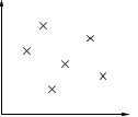
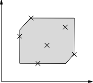
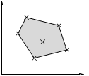
Figure 2: (a) A set of points in 2D and its approximation using a (b) zone and (c) polygon region.

We review the problem of learning convex geometric invariants. Figure 2 visualizes these invariants, showing 2D points (panel a) and two examples of increasingly precise, but also increasingly expensive, convex shapes containing those points (panels b and c). The inferred invariants correspond to the relations defining the enclosing shapes given the trace points from panel a.

The dynamic analysis tool DIG [30, 31] generates different forms of polynomial invariants by building geometric shapes, such as those shown in Figure 2, enclosing the trace points. DIG first determines if the points lie in a simple hyperplane. If such a plane does not exist, DIG then computes a convex hull over the trace points. Such hulls are bounded convex polyhedra—each polyhedron is enclosed by a finite number of facets and contains the line joining any pair of its points. The half-space representation of such a polyhedron is a set of finite linear relations of the form $c_{1}v_{1}+\dots+c_{n}v_{n}\geq c_{0}$. The facets of the polyhedron, corresponding to the solutions of the set of linear inequalities, give a set of candidate inequality invariants among the variables $v_{i}$. Figure 2c shows a 2D polyhedron with five facets, represented by five linear inequalities. For efficiency, DIG also considers more restricted forms of inequalities representing simpler geometric shapes, such as the six-edged zone relation [9, 29] in Figure 2b and the eight-edged octagon relation [9].

To support nonlinear relations, DIG lifts its analysis to terms representing nonlinear polynomials over program variables. For example, rather than analyzing variables $v_{1}$ and $v_{2}$ directly, relations can be constructed among the terms $t_{1}=v_{1},t_{2}=v_{1}v_{2}$ (note that $t_{2}$ is nonlinear). Thus, equations such as $t_{1}+t_{2}=1$ can be generated, which represents a line over $t_{1},t_{2}$ but a hyperbola over $v_{1},v_{2}$. When additional traces are available, filtering step removes spurious invariants [30].

These existing approaches lack the expressive power to learn disjunctive invariants, a gap that we address in the following subsection by reformulating in the max-plus algebra.

3.2 Max-Plus Invariants

As discussed earlier, programs containing loops or conditional branches are not adequately modeled by purely conjunctive invariants. Figure 1 depicts the nonconvex region defined by the loop invariant $(x<5\wedge y=5)\vee(5\leq x\leq 11\wedge x=y)$ in our program ex1. Such disjunctive information cannot be expressed as a conjunction of polynomial relations, including octagon or even general polyhedron forms. Although disjunctive invariants can be simulated using polynomials of higher order (e.g., $a=0\vee b=0$ is equivalent to $a\times b=0$), this approach generates terms with impractically high degree and computational cost, especially when there are more than two disjunctions. We thus require a fundamentally different approach.

To model disjunctive invariants, we use formulas representing max-plus polyhedra [1], i.e., nonconvex hulls that are convex over a max-plus algebra. Max-plus formulas allow disjunctions of zone relations [9, 29]: inequalities of the forms $\pm v\geq c$ and $v_{1}-v_{2}\geq c$. Formally, max-plus relations have the structure

$$\begin{array}[]{l}\max(c_{0},c_{1}+v_{1},\dots,c_{n}+v_{n})\geq\\ \max(d_{0},d_{1}+v_{1},\dots,d_{n}+v_{n}),\end{array}$$

where $v_{i}$ are program variables, $c_{i},d_{i}$ are real numbers or $-\infty$, and $\max(t_{0},\dots,t_{m})$ returns the largest $t_{i}$. That is, $\max(x,y)\equiv\mathsf{if}\;x>y\;\mathsf{then}\;x\;\mathsf{else}\;y$. We note that $\max(v_{0},v_{1}-\infty,v_{2},\dots,v_{n})=\max(v_{0},v_{2},\dots,v_{n})$ and thus we often drop $-\infty$ $\max$-arguments.

The $\max$ operator allows max-plus formulas to encode certain disjunctions. For example, the max-plus relation $\max(0,x-5,y-\infty)=\max(-\infty,x-\infty,y-5)$, i.e., $\max(0,x-5)=\max(y-5)$, encodes the disjunction $(5>x\wedge y=5)\vee(5\leq x\wedge x=y)$, or $y=5\vee x=y$.

Max-plus relations are analogous to polyhedra relations, but use $(\max,+)$ instead of the $(+,\times)$ of standard arithmetic. These operators allow max-plus relations to form geometric shapes that are nonconvex in the classical sense. For example, the max-plus relation $x=y\vee y=5$ represents a nonconvex region consisting of two lines $x=y$ and $y=5$. Moreover, the structure of max-plus relations produces a relatively peculiar geometric shape. Figure 3a shows the three possible shapes of a max-plus line segment in 2D. In general dimensions, two points are always connected by lines that run parallel, perpendicular, or at a 45 degree angle to all the coordinate axes. A max-plus polyhedron consists of these connections and the area surrounded by them. Figure 3b depicts a max-plus polyhedron represented by a set of four lines connecting the four marked points. Although a max-plus polyhedron is not convex in the classical sense, it is convex in the max-plus sense using max-plus algebra. That is, it contains any max-plus line segment between any pair of its points. This allows us to generate max-plus polyhedra over a finite set of traces, as shown in Figure 3b. Where there is no confusion, we shorten max-plus (resp. min-plus) to max (resp. min) when describing polyhedra, formula, or relations.

Figure 3: (a) Three possible shapes of a max-plus line segment: $\max(x+a,b)\geq y$ (top), $\max(y+a,b)\geq x$ (right), $\max(x+a,y+b)\geq c$ (left) and (b) a max-plus convex hull built over four points using these line segments.

A bounded max polyhedron can have finitely many facets representing max relations, e.g., even a 2D complex polygon may contain multiple edges. Thus, a disjunctive formula representing a max polyhedron has no fixed bounds on the number of disjuncts used. However, computing a max polyhedron over $n$ points in $d$ dimensions is computationally expensive $O(n^{d})$ [1], similar to classical polyhedron computations. Next, we propose heuristics to avoid generating these high-dimensional polyhedra in Section 3.3. Section 3.4 then introduces a simpler form of max relations that strikes a reasonable compromise between efficiency and precision.

3.3 Dynamically Inferring Max-Plus Invariants

input : set of variables $V$, set of traces $X$, max degree $d$

output : set $S$ of polynomial inequalities

$T\leftarrow$ genTerms($V$,$d$)

$P\leftarrow$ genPoints($T$,$X$)

$H\leftarrow$ createMaxPlusPolyhedron($P$)

$S\leftarrow$ extractFacets($H$)

return $S$

Algorithm 1 High-level algorithm for finding disjunctive polynomial inequalities.

We infer max invariants dynamically using a procedure similar to that used for classical polyhedra invariants. Figure 1 outlines the main steps of the algorithm: using terms to represent program variables; instantiating points from terms using input traces; creating a max polyhedron enclosing the points; and extracting its facets to represent max relations among terms.

Because program invariants often involve only a small subset of all possible program variables, we employ heuristics to search iteratively for invariants containing all possible combinations of a small, fixed number of variables. We propose to consider max relations over triples of program variables, i.e., $\max(c_{0},c_{1}+v_{1},c_{2}+v_{2},c_{3}+v_{3})\geq\max(d_{0},d_{1}+v_{1}+d_{2}+v_{2},d_{3}+v_{3})$ representing max polyhedra in three-dimensional space.

Our algorithm also supports nonlinear max relations by using terms to represent nonlinear polynomials over variables. However, the number of possible terms is exponential in the number of degrees [30] and thus we target linear max relations by default for efficiency. The user of DIG can change the parameter $d$ in Figure 1 to generate higher degree relations (e.g., $d=2$ for quadratic relations) and can also manually define terms to capture other desirable properties. For example, a user with knowledge about the shape of the desired invariants might hypothesize a spherical shape $\max(c_{0},c_{1}+x^{2},c_{2}+y^{2})\geq\max(d_{0},d_{1}+x^{2},d_{2}+y^{2})$. With that as input, the algorithm searches for that exact shape (i.e., computes the coefficients $c_{i},d_{i}$) from the polyhedron built over the trace points of the terms representing the nonlinear polynomials $x^{2}$ and $y^{2}$.

Example

We illustrate the algorithm by deriving the invariant $(x<5\wedge y=5)\vee(5\leq x\leq 10\wedge x=y)$ at location $L$ in program ex1 in Figure 1. The trace values for $x,y$ in Figure 1 form a set of eleven points (e.g., the first is $(-1,5)$). We then compute a max polyhedron over these points. The half-space representation of that polyhedron consists of the max relations:

$$\small\begin{array}[]{ccccc}11&\geq&x&\geq&-1\\ 11&\geq&y&\geq&5\\ 0&\geq&x-y&\geq&-6\\ \max(0,x-5)&\geq&y-5\end{array}$$

The conjunction $0\geq x-y\;\wedge\;11\geq x\;\wedge\;\max(x-5,0)\geq y-5$, which forms the nonconvex region in Figure 1, is logically equivalent to the invariant $(x<5\wedge 5=y)\vee(5\leq x\leq 11\wedge x=y)$.

Note that $x\geq-1$ and $x-y\geq-6$ are spurious relations because $x$ has no lower bound. Additional traces, such as running ex1 on $x=-5$, would remove these spurious invariants. More generally, the static technique in Section 4 formally verifies candidate invariants and removes spurious results.

3.4 Weak Max-Plus Invariants

We introduce and define a weaker form of max relations that retains much expressive power but avoids the high computational cost of computing a max polyhedron. Our approach is inspired by earlier methods for finding simpler forms of inequalities (e.g., zone and octagon) to avoid the cost of finding general polyhedra [29]. To the best of our knowledge, this is the first attempt to consider a simpler form of max inequalities for program analysis.

We define a weak max relation to be of the form:

$$\begin{array}[]{l}\max(c_{0},c_{1}+v_{1},\dots,c_{k}+v_{k})\geq v_{j}+d,\\ v_{j}+d\geq\max(c_{0},c_{1}+v_{1},\dots,c_{k}+v_{k}),\end{array}$$

where $v_{i}$ are program variables, $c_{i}\in\{0,-\infty\}$, $d$ is a real numbers or $-\infty$, and $k$ is a constant, e.g., $k=2$. Unlike general max relations, weak max relations have some convenient properties:

1. They restrict the values of the coefficients $c_{i}$ to $\{0,-\infty\}$. The general form allows $c_{i}\in\mathbb{R}\cup\{-\infty\}$.

2. They fix the number of variables $k$ to a small constant. The general form allows $n$ variables.

3. They allow only one unknown parameter $d$. The general form allows $d_{0}\dots d_{n}$.

Weak max relations are thus a strict subset of general max relations. For example, the weak max form cannot represent general max relations like $\max(x+7,y)\geq z$ or $\max(x,y)\geq\max(z,w)$, but it does support zone relations like $x-y\geq 10,x=y$ and disjunctive relations like $\max(x,y)\geq z$ and $\max(x,0)\geq y+7$.

Geometrically, weak max relations are a restricted kind of max polyhedra. While general max line segments have the possible three shapes shown in Figure 3, weak max line segments have only two shapes represented by the formulas $\max(x,b)\geq y$ and $\max(y,b)\geq x$. That is, weak max shapes include only lines that run in parallel or at a 45 degree angle. Lines with a perpendicular shape cannot occur because their formula, $\max(x,y)\geq 0$, is inexpressible using the weak max form.

The advantage of these restrictions is that they admit a straightforward algorithm to compute the bounded weak max polyhedron over a set of finite points in $k$ dimensions. The algorithm first enumerates all possible weak relations over $k$ variables and then finds the unknown parameter $d$ in each relation from the given points. The resulting set of relations is the half-space representation of the weak max polyhedron enclosing the points.

Note that this algorithm does not apply to the general max form because the coefficients $c_{i}$ are not enumerable over the reals. Moreover, the problem becomes more complex when more than one unknown is involved. For instance, it is nontrivial to compute the unknowns $c,d$ in the max relation $\max(c,x)\geq y+d$ because the values of $c$ and $d$ depend on each other.

Example

We illustrate this algorithm by finding the weak max polyhedron enclosing the points $\{(x_{1},y_{1}),\dots,(x_{n},y_{n})\}$ in 2D. First, we enumerate relations of the weak max form by instantiating the coefficients $c_{i}$ over $\{0,-\infty\}$. For the form $\max(c_{0},c_{1}+x,c_{2}+y)\geq x+d$ we obtain eight max relations (two choices each for three coefficients):

$$\small\begin{array}[]{lr}\max(0,x,y)\geq x+d,&\dots\\ \max(0,x)\geq x+d,&-\infty\geq x+d\\ \end{array}$$

The eight additional max relations for each of the other three forms $\max(c_{0},c_{1}+x,c_{2}+y)\geq y+d$, $x+d\geq\max(c_{0},c_{1}+x,c_{2}+y)$, $y+d\geq\max(c_{0},c_{1}+x,c_{2}+y)$ are obtained similarly. Redundant relations can be removed (e.g., $\max(y,0)\geq x$ implies $\max(x,y,0)\geq x$).

Next, we compute the parameter $d$ in each of the 32 obtained relations using the given points $\{(x_{1},y_{1}),\dots,(x_{n},y_{n})\}$. For instance, $\max(y,0)\geq x+d$ has $d=\min(\max(y_{i},0)-x_{i})$ and $x+d\geq\max(y,0)$ has $d=\max(\max(y_{i},0)-x_{i})$. The resulting relations form an intersecting region that represents a bounded weak max polygon over the given points.

In general, the number of weak max relations enumerated over $k$ variables is $O(k2^{k+2})$ and the time to find the single parameter $d$ in each relation is linear in the number of points. Thus, the complexity for computing a weak max polyhedron over $n$ points in $k$ dimensions is $O(n2^{k})$. The complexity is therefore polynomial in the number of points when $k$ is a constant and is exponential in the number of dimensions when $k$ is not fixed. Note that even this worst case is still smaller than $O(n^{d})$, the complexity of building a general max polyhedron. Importantly, the number of facets of a weak max polyhedron has a fixed upper bound for each $k$. For example, $k=2$ has at most 32 facets. This is thus more manageable than the number of facets of general max polyhedron, which can be arbitrarily finitely many.

3.5 Min-Plus Invariants

We also consider min relations of the form

$$\begin{array}[]{l}\min(c_{0},c_{1}+v_{1},\dots,c_{n}+v_{n})\geq\\ \min(d_{0},d_{1}+v_{1},\dots,d_{n}+v_{n}),\end{array}$$

where $v_{i}$ are program variables and $c_{i},d_{i}\in\mathbb{R}\cup\{\infty\}$. Similar to its max dual, a min polyhedron is a formed by the intersection of finite min lines. However, min and max relations describe different forms of disjunction information and have different geometric shapes. For instance, the relation $\min(x,y)=z$ encodes the disjunction $(x<y\Rightarrow x=z)\wedge(x\geq y\Rightarrow y=z)$ that is not expressible as a max relation. Figure 4 depicts the min version of the shapes in Figure 3.

Figure 4: (a) Three possible shapes of a min-plus line segment and (b) a min-plus polyhedron built over four points.

A conjunction of max and min invariants can describe information that is inexpressible using either max or min relations alone. Consider program ex2 in Figure 5, which has the invariant $y\leq 10\Leftrightarrow b=0$ at location $L$. By building max and min polyhedra over the traces given in Figure 5, we obtain $1\geq b\geq 0$, $\max(y-10,0)\geq b$, and $b+10\geq\min(y,11)$. Given $1\geq b\geq 0$, the max relation implies $b=0\Rightarrow y\leq 10$ and the min relation implies $b\neq 0\Rightarrow y>10$. These disjunctions are mathematically equivalent to the $\mathsf{iff}$ condition $y\leq 10\Leftrightarrow b=0$.

⬇

int ex2(int x){

int y, b;

if (x>=0) {y=x+1;}

else {y=x-1;}

b=(y>10);

[L]

return b;

}

$x$	$y$	b
-50	-51	0
-33	-34	0
9	10	0
10	11	1
12	13	1
40	41	1

Figure 5: Program ex2 and its trace data at location $L$ for several input values.

Dually, we also define weak min relations:

$$\begin{array}[]{l}\min(c_{0},c_{1}+v_{1},\dots,c_{k}+v_{k})\geq v_{j}+d_{i},\\ v_{j}+d_{i}\geq\min(c_{0},c_{1}+v_{1},\dots,c_{k}+v_{k}),\end{array}$$

where $v_{i}$ are program variables, $k$ is a constant, $c_{i}\in\{0,-\infty\}$, and $d_{i}\in\mathbb{R}\cup\{-\infty\}$. The algorithm for computing weak min polyhedra over finite points is similar to the one for weak max polyhedra and has equivalent theoretical complexity as given in Section 3.4.

3.6 Algorithmic Analysis

We analyze important properties associated with our algorithm. There are two key concerns: the production of spurious invariants that underapproximate general program behavior (too strong relations that hold only for some inputs) and invariants that overapproximate general program behavior (weak invariants that may not be useful).

By building max or min polyhedra over trace points, which are convex in the corresponding max or min algebra, our algorithm guarantees that it produces candidate invariants that always underapproximate, or are equivalent to, program invariants expressible under the max or min-plus forms. The proof of this claim follows from the facts that (1) the given set of observed traces is a subset of all possible program traces and (2) our constructed max polyhedron over a set of points is the smallest max polyhedron represented by those points. The proof details follow those of the underapproximation argument for inferring classically convex shapes [31]. Thus, if the program invariants are expressible in our system, our algorithm never overapproximates.

This underapproximation property is important because its violation—a candidate invariant strictly overapproximating the program invariant—indicates a bug in the subject program. For example, if the expected invariant is $t\geq 1$ but our algorithm discovers $t\geq 0$, then the underapproximation property guarantees the value $t=0$ exists in the observed traces. The trace with $t=0$ represents a counterexample that violates the expected property of $t$ being positive.

Underapproximation properties also represent spurious invariants. One way of understanding why spurious results occur is that (1) a max or min polyhedron has many facets in high-dimensional space, and (2) inadequate traces may result in a constructed polyhedra with facets representing spurious relations. For instance, if $x,y$ can take any value over the reals, then an $n$-facet max polygon built over any set of trace points for $x,y$ produces $n$ spurious invariants because no bounded max-plus polygons can capture the unbounded ranges of $x,y$. Both filtering against additional traces and restricting attention to the weaker forms of max and min relations help reduce spurious invariants. In the next section we describe a more general technique, based on theorem proving, to distinguish between true and spurious invariants.

4 Verifying Candidate Invariants

Our algorithm, and convex hull methods in general, can generate many powerful but potentially incorrect relations due to trace incompleteness. We augment dynamic invariant generation with static theorem proving to produce sound program invariants with respect to the program source code. Specifically, we verify program invariants using $k$-induction. In this approach, $k$ base cases are specified, and the $k$ previous instances are available for proving the inductive step (e.g., [16]). This additional power allows us to prove many invariants relevant to program verification that do not admit standard induction.

Our theorem prover design, called KIP, is based on iterative $k$-induction and uses SMT solving to verify candidate invariants. In addition, its architecture supports parallel checking of invariants, dramatically improving efficiency. Recent advances in SMT solving [23, 34, 13] allow for efficient analysis over formulas encoding complex programs and properties in powerful theories. This means that we can reason about, and verify, invariants involving theories such as nonlinear arithmetic and data structures such as arrays, bit vectors, and pointers.

⬇

int sqrt(int x){

assert(x>=0);

int a=0,s=1,t=1;

while[L](s<=x){

a += 1;

t += 2;

s += t;

}

return a;

}

Consider the program sqrt on the right, which computes the square root of an integer using only addition. From observed traces at location $L$, our algorithm generates candidate loop invariants such as $t=2a+1,4s=t^{2}+2t+1,s=(a+1)^{2},s\geq t$ and $x\leq 9989$. KIP successfully distinguishes true and false invariants from these results. Specifically, we prove $t=2a+1$ and $4s=t^{2}+2t+1$ are inductive invariants and $s=(a+1)^{2}$ is a $1$-inductive invariant (i.e., cannot be proved using standard induction). By using proved results as lemmas, KIP is able to show the invariant $s\geq t$, which is not $k$-inductive for $k\leq\mathsf{maxK}$, where $\mathsf{maxK}=5$ is the default setting of KIP. The prover also rejects spurious relations such as $x\leq 9989$ by producing counterexamples that invalidate those relations in sqrt. The parallel implementation allows the prover to check these candidate results simultaneously.

4.1 Analyzing Programs using $k$-Induction

A program execution can be modeled as a state transition system $M=(I,T)$ with $I$ representing the initial state of $M$, and $T$ specifying the transition relation of $M$ from a state $n-1$ to a state $n$. To prove that $p$ is a state invariant that holds at every state of $M$, $k$-induction requires that $p$ hold for the first $k+1$ states (base case) and that $p$ hold for the state $n+k+1$ assuming that it holds for the $k+1$ previous states (induction step). Formally, $k$-induction proves the state invariant $p$ of $M=(I,T)$ by checking the base case and induction step formulas:

$$I\wedge T_{1}\wedge\dots\wedge T_{k}\; \Rightarrow\;p_{0}\wedge\dots\wedge p_{k}$$ (1)

$$p_{n}\wedge T_{n+1}\wedge\dots\wedge p_{n+k}\wedge T_{n+k+1}\; \Rightarrow\;p_{n+k+1}$$ (2)

If both formulas hold then $p$ is a $k$-inductive invariant. If the base case (1) fails then $p$ is disproved and thus is not an invariant (assuming that $M$ correctly models the program). However, if the base case holds but the induction step (2) fails, then $p$ is not a $k$-inductive invariant, but it could still be a program invariant. Thus, $k$-induction is a sound but incomplete proof technique.

By considering multiple consecutive transitions, $k$-induction can prove invariants that cannot be proved by standard induction ($0$-induction in this formulation). For instance, the invariant $x\neq y$ of the machine $M(I:(x=0\wedge y=1\wedge z=2)_{0}$, $T_{n}:x_{n}=y_{n-1}\wedge y_{n}=z_{n-1}\wedge z_{n}=x_{n-1}$) that rotates the values $0,1,2$ through the variables $x,y,z$ is not provable by standard induction but is $k$-inductive with $k\geq 3$. The notation $(P)_{i}$ denotes the formula $P$ with all free variables subscripted by $i$, e.g., $(x+y=1)_{0}$ is $x_{0}+y_{0}=1$.

4.2 $k$-Induction and SMT Solving

input : $\mathit{I,T,p}$

output : $\{\mathit{proved,disproved,unproved}\}$

for $\mathit{k=0}$ to $\mathsf{maxK}$ do

      

      // base case

      

      if $\mathit{k=0}$ then $\mathit{S_{b}.assert(I)}$

       else $\mathit{S_{b}.assert(T_{k})}$

      

      if $\mathit{\neg S_{b}.entail(p_{k})}$ then  return ($\mathit{disproved,S_{b}.cex}$)

      

      // induction step

       $\mathit{S_{s}.assert(p_{k},T_{k+1})}$

       if $\mathit{\neg S_{s}.entail(p_{k+1})}$ then return $\mathit{proved}$

      

return $\mathit{unproved}$

Algorithm 2 Procedure $\mathsf{kprove}$ for incremental $k$-induction using SMT solvers $S_{b}$ and $S_{s}$.

Figure 2 outlines the procedure for verifying a property $p$ using inductive $k$-induction with SMT solving. The procedure consists of a loop that performs incremental $k$-induction, starting from $k=0$. The loop terminates when either the base case fails ($P$ is not an invariant), both the base case and the induction step hold ($P$ is an invariant), or $\mathsf{maxK}$ is reached ($P$ is not a $\mathsf{maxK}$-inductive invariant).

We use two independent SMT solvers $\mathit{S_{b}}$ and $\mathit{S_{s}}$ to check the two formulas corresponding to the base case (1) and induction step (2). For a solver $S$ and a formula $f$, we append $f$ to $S$ through assertion and check if the assertions in $S$ imply $f$ using entailment [13]. If $S$ does not entail $f$, then the solver returns a counterexample (cex) satisfying $a_{1}\wedge\dots\wedge a_{n}$ but not $f$.

4.3 The Architecture of KIP

input : $\mathit{S,L,P}$

output : $\mathit{P_{i},P_{r},P_{d},P_{u}}$

$\mathit{I,T\leftarrow vcgen(S,L)}$

$\mathit{P_{p}\leftarrow\emptyset;P_{d}\leftarrow\emptyset;P_{u}\leftarrow\emptyset}$

repeat

      

      $\mathit{New_{p}\leftarrow\emptyset;New_{u}\leftarrow\emptyset}$

      

      foreach $\mathit{p\in P}$ do

             $\mathit{r\leftarrow kprove(I,T,p)}$

            

            if $\mathit{r=proved}$ then

                   $\mathit{P_{p}.add(p)};\mathit{New_{p}.add(p)}$

                  

            else if $\mathit{r=unproved}$ then  $\mathit{New_{u}.add(p)}$

            

             else $P_{d}.add(p)$

            

      

      $\mathit{KIP.addLemmas(New_{p})}$

       $\mathit{P\leftarrow New_{u}}$

      

until $\mathit{New_{p}=\emptyset\;\vee\;New_{u}=\emptyset}$

$\mathit{P_{u}\leftarrow P}$

$P_{i},P_{r}=check\_redundancy(P_{p})$

return $P_{i},P_{r},P_{d},P_{u}$

Algorithm 3 Procedure to verify candidate invariants. $P_{i}$ and $P_{r}$ are proved results, however $P_{r}$ are redundant because $P_{i}\Rightarrow P_{r}$. $P_{d}$ and $P_{u}$ are disproved and unknown results, respectively.

At a high level, verifying a candidate invariant against a program requires two steps: (1) computing a formula that encodes the program’s semantics; and (2) proving whether the candidate invariant is consistent with that formula or not. To increase expressive power in practice, we also (3) incorporate knowledge of all invariants learned thus far.

Figure 3 outlines the architecture of KIP, our $k$-inductive parallel theorem prover, to verify a set $P$ of candidate obtained at location $L$ for program $S$. We first generate from the program $S$ and the location $L$ the formulas $I,T$. These formulas can be thought of as representing the state transition system $M=(I,T)$ described above. Equivalently, $I,T$ can be thought of as verification conditions (vcs) based on weakest preconditions (wps) from program analysis using Hoare logic.

The backward analysis method [15] provides the necessary rules to create $I,T$ for imperative programming constructs such as assignments, conditional branches, and loops. This area is well-established—tools such as Microsoft Boogie [27] and ESC [14] implement various methods based on backward analysis to automatically generate vcs using wps.

Our algorithm progresses by trying to prove the invariants in the context of the vcs. While unproved invariants remain, the procedure attempts to re-prove them by adding newly proved results as lemmas to KIP. In many cases, this additional knowledge allows KIP to prove properties that could not be proved previously (see Sections 2 and 5.2). A disproved invariant is likely spurious (e.g., assuming $I,T$ correctly models the program), a proved invariant is definitely correct, and an unproved invariant (e.g., one that is not $\mathsf{maxK}$-inductive) can be conservatively rejected.

The algorithm supports parallelism, which can check candidate invariants (the for loop in Figure 3) simultaneously using multiple threads. In a post-processing step, KIP uses implication to partition all proved invariants into two sets: those that are independent (i.e., strongest) and those that can be implied by the others (i.e., weaker). The implied invariants are redundant and need not be presented to the developer. This partitioning uses the backend SMT solver to check if each invariant $p\in P_{p}$ can be inferred by the conjunction of other proved invariants $P_{p}\setminus\{p\}$.

Overall, KIP’s design represents a novel combination of established techniques and provides the five properties we desire for the efficient verification of complex invariants: (1) use of $k$-induction for expressive power; (2) use of SMT solvers for reasoning about program-critical theories like nonlinear arithmetic; (3) learning of lemmas to prove otherwise non-inductive properties; (4) explicit parallelism for performance; and (5) removing weaker implied results for human consumption.

5 Experimental Evaluation

This section evaluates the efficiency and expressive power of our methods. We consider the research questions:

• RQ1: Can the hybrid algorithm efficiently generate powerful disjunctive invariants and prove them correct?

• RQ2: Is the hybrid algorithm effective on complex correctness properties, such as those that are not classically inductive or involve nonlinear arithmetic?

To investigate RQ1 we applied our algorithms to a Disjunctive Invariant benchmark suite of kernels involving abstractions of string and array processing. To investigate RQ2 we used a Nonlinear Arithmetic benchmark suite. Each program comes equipped with “gold standard” full-correctness annotations (e.g., assertions, postconditions, or formalized documented invariants).

Each program was run on 300 random inputs to provide traces for invariant generation and 100 random inputs for filtering, as described in [30]. For small kernels, this yields sufficient traces to generate accurate invariants [38, 33]. Our test programs come with annotated invariants at various locations such as loop heads and function exits. For evaluation purpose, we instrumented the values of variables at those locations and find invariants among the resulting traces. We use only the weak max and min forms given in Section 3.4 unless the number of variables is three or less, in which case it is also practical to use the general forms.

We implemented our algorithms in the dynamic analysis framework DIG [30, 31] using the Sage mathematical environment [40]. Our prototype uses the Tropical Polyhedra Library TPLib [2] to manipulate max and min polyhedra and uses built-in Sage functions to solve equations and construct convex hulls for classical polyhedra. The prototype KIP prover uses Z3 [13] to check the satisfiability of SMT formulas. As mentioned, we consider linear max-plus relations and set $\mathsf{maxK}=5$ by default. The prototype constructs the verification conditions corresponding to $M=(I,T)$ (Section 4.3) directly; a more efficient tool such as Microsoft Boogie could also be used. The experiments were performed on a 64-core 2.60GHz Intel Linux system with 128 GB of RAM; KIP used 64 threads of parallelism.

Table 1: Disjunctive Invariant experimental results.

Prog	Loc	Var	Gen	T${}_{\text{Gen}}$	Val	T${}_{\text{Val}}$	Hoare
ex1	1	2	15	0.2	4	1.5	✓
strncpy	1	3	69	1.1	4	7.7	✓
oddeven3	1	6	286	3.7	8	16.0	✓
oddeven4	1	8	867	12.7	22	46.0	✓
oddeven5	1	10	2334	56.8	52	1319.4	✓
bubble3	1	6	249	4.1	8	4.9	✓
bubble4	1	8	832	11.7	22	47.6	✓
bubble5	1	10	2198	53.9	52	938.2	✓
partd3	4	5	479	10.5	10	50.8	✓
partd4	5	6	1217	23.3	15	181.1	✓
partd5	6	7	2943	53.3	21	418.1	✓
parti3	4	5	464	10.3	10	45.5	✓
parti4	5	6	1148	22.4	15	165.1	✓
parti5	6	7	2954	53.6	21	405.6	✓
total			16055	317.6	264	3647.5	14/14

5.1 RQ1: Disjunctive Invariants

We evaluate our approach on several benchmark kernels for disjunctive invariant analysis [1], listed in Table 1. These programs typically have many execution paths, e.g., oddeven5 contains 12 serial “if” blocks and thus $2^{12}$ paths. The documented correctness assertions for these programs require reasoning about disjunctive invariants, but do not involve higher-order logic. For example, the sorting procedures are asserted to produce sorted output, but are not asserted to produce a permutation of the input.

Table 1 report experimental results. The Loc column lists the number of locations where invariants were generated. The Var column reports the number of distinct variables involved in the invariants. The Gen column counts the number of unique candidate invariants generated by our dynamic algorithm. The T${}_{\text{Gen}}$ column reports the generation and filtering time, in seconds, averaged over five runs. The number of generated invariants speaks to the expressive power of the algorithm: higher is better, indicating that we can reason about more disjunctive relationships over program variables. Time indicates the efficiency of our algorithm: lower is better. The Val column reports the number of generated invariants that KIP proved correct and non-redundant with respect to the program. The other generated invariants were disproved three times as often as they were proved redundant. A few invariants, just under 2% on average, could neither be proved nor disproved. The T${}_{\text{Val}}$ column counts the time, in seconds, to analyze all of the generated invariants.

We desire validated invariants to statically prove each program’s annotated correctness condition via Hoare logic. The Hoare column indicates whether the validated invariants were sufficient to prove program correctness. For all of these programs, the invariants generated and validated by our hybrid approach—an average of 18 per programs—were sufficient for a static proof of full correctness.

For example, for the C string function strncpy, which copies the first $n$ characters from a (null-terminated) source $s$ to a (unconstrained) destination $d$, we inferred the relation:

$$\small(n\geq|s|~{}\wedge~{}|d|=|s|)~{}\vee~{}(n<|s|~{}\wedge~{}|d|\geq n)$$

This captures the desired semantics of the function: if $n\geq|s|$, then the copy stops at the null terminator of $s$, which is also copied to $d$, so $d$ ends up with the same length as $s$. However, if $n<|s|$, then the terminator is not copied to $d$, so $|d|\geq n$.

As a second example, for bubble_N and oddeven_N, which sort the input elements $x_{0},\dots,x_{N}$ and store the results in $y_{0},\dots,y_{N}$, our inferred invariants prove the outputs $y_{0}$ and $y_{N}$ hold the smallest and largest elements of the input. However, we cannot show that $y$ is a permutation of $x$ because that is expressible only under higher-order logics (our results here are similar to those of purely static analyses [1]).

Table 1 shows that our method is efficient. We can infer about 3000 disjunctive relations per minute, on average, and validate about 300 per minute. The method is also effective. We produced 264 non-redundant, proved-correct disjunctive invariants, and those invariants were sufficient to statically prove each program’s contract.

5.2 RQ2: Complex Invariants

Table 2: Nonlinear Arithmetic experimental results.

Prog	Loc	Var	Gen	T${}_{\text{Gen}}$	Val	$k$I	T${}_{\text{Val}}$	Hoare
cohendv	2	6	152	26.2	7	14	8.2	✓
divbin	2	5	96	37.7	8	15	8.7	–
manna	1	5	49	19.2	3	2	5.6	✓
hard	2	6	107	14.2	11	4	9.2	–
sqrt1	1	4	27	25.3	3	1	4.3	✓
dijkstra	2	5	61	30.7	8	6	10.9	–
freire1	1	3	25	22.5	2	0	2.2	✓
freire2	1	4	35	26.0	3	1	5.1	✓
cohencb	1	5	31	23.6	4	1	4.2	✓
egcd1	1	8	108	43.1	1	8	12.8	–
egcd2	2	10	209	60.8	8	12	14.6	✓
egcd3	3	12	475	67.0	14	25	23.4	✓
lcm1	3	6	203	38.9	12	0	14.2	✓
lcm2	1	6	52	14.9	1	10	0.9	✓
prodbin	1	5	61	28.3	3	10	1.1	–
prod4br	1	6	42	9.6	4	7	8.6	✓
fermat1	3	5	217	75.7	6	1	6.2	✓
fermat2	1	5	70	25.8	2	0	5.2	✓
knuth	1	8	113	57.1	4	6	24.6	✓
geo1	1	4	25	16.7	2	4	1.5	✓
geo2	1	4	45	24.1	1	10	2.1	✓
geo3	1	5	65	22.1	1	12	2.7	✓
ps2	1	3	25	21.1	2	0	4.0	✓
ps3	1	3	25	21.9	2	0	4.2	✓
ps4	1	3	25	23.5	2	0	4.9	✓
ps5	1	3	24	24.9	2	0	7.4	✓
ps6	1	3	25	25.0	2	0	69.5	✓
total			2392	825.9	118	149	266.3	22/27

We also evaluate our technique on more complex programs, such as those that are not classically inductive or use nonlinear arithmetic, by studying the NLA (nonlinear arithmetic) test suite [30]. The suite consists of 27 programs from various sources collected by Rodríguez-Carbonell and Kapur [6, 36, 5]. The programs are relatively small, on average two loops of 20 lines of code each. However, they implement nontrivial mathematical algorithms and are often used to benchmark static analysis methods. For these programs, we generate and check loop invariants of two polynomial forms: nonlinear equations and linear max-plus inequalities among program variables. We consider at most 200 generated terms per polynomial equality, e.g., invariants up to degree five if four variables are involved. The documented correctness assertions for these 27 programs require nonlinear invariants, mostly equalities among nonlinear polynomials.

Table 2 shows the results, in a format similar to that of Table 1. The large number of candidate invariants generated—over 80 per program, on average—highlights the expressive power of our technique. The generation is slightly slower than for the disjunctive benchmarks because these require equation solving for large numbers of terms representing nonlinear polynomials. However, our weak forms take an order of magnitude less time than do the general equality relations. The overall generation process remains efficient, averaging thirty seconds per program.

Our hybrid approach is able to formally validate 118 of those invariants, or 4.3 per program on average, proving them correct and non-redundant. The validation is rapid (0.1 seconds per candidate invariant, on average, compared to 0.2 for the disjunctive benchmarks) but here shows its reliance on the underlying SMT theorem prover. For 18 of these 27 programs, some of the theorem prover queries issued caused the Z3 SMT solver to return an unknown error or stop responding. This is likely due to the recent addition of support for nonlinear arithmetic, and we reported these errors to the Z3 developers. In the interim, however, such candidate invariants must be rejected.

The $k$I column in Table 2 counts the number of invariants that require $k$-induction to be proved or disproved. Similarly, an additional 39 of the proved invariants required considering discovered invariants as lemmas, and were not otherwise $\mathsf{maxK}$-inductive. The significant presence of invariants requiring $k$-induction or learned lemmas validates the KIP architecture design choice.

Ultimately, the invariants generated and validated by our technique can be used to statically prove the correctness of 22 of these 27 programs using Hoarse logic. Of the remainder, two require novel invariant forms, one requires invariants that are not $k$-inductive, and two are correct but beyond our current SMT solver. For the first type, divbin requires the invariant $\exists k.x=2^{k}$, and our algorithm does not support exponential forms. The hard program also has similar exponential invariants. For the second type, our dynamic algorithm generates three non-linear equalities that precisely capture egcd1’s semantics, and manual inspection verifies that they are not $k$-inductive for any $k$, and thus KIP cannot prove them. For the third type, our dynamic algorithm generates invariants that precisely capture the semantics of prodbin and dijkstra and KIP can process them, but the backend SMT solver hangs instead of proving them (we have manually verified that they are otherwise correct). Thus we could prove two more programs with a better SMT solver, two more programs with a better theorem prover architecture, and could not prove the last without a new algorithm for invariant generation.

6 Related Work

Dynamic invariant analyses. Daikon [18] is a popular and influential dynamic invariant analysis that infers candidate invariants using templates. Daikon comes with a large list of invariant templates and returns those that hold over a set of program traces. Daikon can use “splitting” conditions [17] to find disjunctive invariants such as “$\mathsf{if}\;c\;\mathsf{then}\;a\;\mathsf{else}\;b$”. Our algorithm does not depend on splitting conditions and our max- and min-plus disjunctive invariants are more expressive than those currently supported by Daikon.

Recently, Sharma et al. [38] proposed a machine-learning based approach to find disjunctive invariants. Their method operates on traces representing good and bad program states: good traces are obtained by running the program on random inputs and bad traces correspond to runs on which an assertion or postcondition is violated. They use a probably approximately correct machine learning model to find a predicate, representing a candidate program invariant, that separates the good and bad traces. For efficiency, they restrict attention to the octagon domain and search only for predicates that are arbitrary boolean combinations of octagon inequalities. Finally, they use standard induction technique to check the candidate invariants using Z3 [13]. While our method shares their focus on disjunctive invariants, a key difference is that the strength of their results depends strictly on existing annotated program assertions. For example, in ex1, if the line assert(y==11) is not provided by the programmer then their method will only produce the trivial invariant $\mathsf{True}$. By contrast, our approach does not make such assumptions about the input program, and in some sense the purpose of our approach is to generate those assertions.

Hybrid approaches. Nimmer and Ernst integrated the ESC/Java static checker framework [32] with Daikon, allowing them to validate candidate invariants using a Hoare logic verification approach. This work is very similar in motivation and architecture to ours. Key differences include our detection of richer disjunctive invariants, our verification with respect to full program correctness (“Rather than proving complete program correctness, ESC detects only certain types of errors” [32, Sec. 2]), and our larger evaluation (our system proves over four times as many non-redundant invariants valid and considers over four times as many benchmark kernels).

Static max-plus analyses. The static analysis work of Allamigeon et al. [1] uses abstract interpretation to approximate program properties under the max- and min-plus domains. In contrast to our work, which computes max-plus formulas from dynamic traces, their method starts directly from a formula representing an initial approximation of the program state space and gradually improves that approximation based on the program structure until a fixed point is reached. As with other abstract interpretation approaches for inferring disjunctive invariants such as [37, 35], their method uses an ad-hoc widening operator to ensure termination.

The recent static analysis work of Kapur et al. [26] uses quantifier elimination to find max invariants over pairs of variables. Their method uses table look-ups to modify max relations based on the program structures (e.g., to determine how the max relation is changed after an assignment $a=a+10$). For scalability the approach restricts attention to specific program constructs. For example, they only support analysis on assignments or guards that do not involve multiplication.

A high-level difference between such techniques and our work is that we focus on the efficient inference of invariants from dynamic traces. More generally, we hypothesize that the weak max and min forms introduced in this paper would allow such static techniques to be practically applied to more general classes of programs.

Uses of $k$-induction. The application of $k$-induction is becoming increasingly popular for formulas that may not admit classic induction. Sheeran et al. applied $k$-induction to verify hardware designs using SAT solvers [39]. The PKIND model checker of Kahsai and Tinelli [24, 25] uses $k$-induction and SAT/SMT solvers to verify synchronous programs in the Lustre language. Recently, Donaldson et al. [16] applied $k$-induction to imperative programs with multiple loops. A key distinction between our KIP architecture and these approaches is that none of them offers all four of the other properties (SMT, lemma re-use, redundancy elimination and parallelism) that we find critical for efficiently verifying large numbers of candidate invariants over programs with complex properties such as nonlinear arithmetic. However, we note that the programs and candidate invariants learned in this paper could serve as a benchmark suite for the evaluation of such theorem provers (i.e., hundreds of valid and invalid formulas involving nonlinear arithmetic, many of which are $k$-inductive).

7 Conclusion

Program invariants are important for defect detection, program verification, and automated repair. Existing approaches struggle with soundness and expressive power and cannot learn disjunctive invariants. We propose a hybrid approach to invariant inference that finds complex invariants dynamically and proves them statically.

We present the first dynamic algorithm to learn the max-plus class of disjunctive invariants, allowing us to capture conditional behavior. To do so, we reformulate the problem of convex invariant detection in a non-standard max-plus algebra. We gain expressive power with dual min-plus constraints, capturing if-and-only-if behavior.

Critically, we also define and infer a new class of weak max- and min-plus invariants that retain useful expressive power while requiring only polynomial complexity. To the best of our knowledge, this is the first use of a restricted form of max- or min-plus invariants.

These weak forms suggest new theoretical research directions for max- and min-plus algebras. Although we provide the algorithm for computing weak relations given points, the dual problem for computing extremal points given relations remains open. The cost of computing general polyhedra inspired general research work on weaker abstract domains (e.g., interval, box, zone and octagon) and formal logic [29]. We see the relationship between our weak max-plus form and general max-plus as analogous to that between octagons and general polyhedra (e.g., fixed coefficients, only one open parameter, etc.), and hope that other max-plus researchers may find our weak form somewhat as useful as polyhedra practitioners have found octagon forms.

We also propose a static approach to invariant verification based on iterative, parallel $k$-inductive SMT theorem proving. Many program invariants are not classically inductive, and $k$-induction allows us to prove them. Similarly, the re-use of learned invariants as lemmas allows our system to prove non-$\mathsf{maxK}$-inductive invariants in practice. Our design’s explicit parallel structure is critical for performance. By construction, our algorithm never overapproximates if the real invariant is expressible in our system, and validating each candidate against the program means that our system never underapproximates: this approach helps address the issue of spurious or incorrect invariants.

We evaluate our algorithm by extending the DIG framework and considering difficult benchmark kernels involving nonlinear arithmetic and abstract arrays. Our approach is efficient and effective at finding and validating disjunctive, non-linear and complex invariants. Ultimately we find and verify invariants that are powerful enough to prove 36 of 41 programs correct using Hoare logic, taking two minutes per program, on average, and producing no spurious answers.

8 ACKNOWLEDGMENTS

Nguyen is grateful for an internship at the Naval Research Laboratory, which introduced him to $k$-induction proving and led to KIP. We thank Matthias Horbach and Hengjun Zhao for insightful discussions. We gratefully acknowledge the partial support of AFORSR (FA9550-07-1-0532, FA9550-10-1-0277), DARPA (P-1070-113237), DOE (DE-AC02-05CH11231), NSF (SHF-0905236, CCF-0729097, CNS-0905222, CCF-1248069, DMS-1217054) and the Santa Fe Institute.

References

- [1] X. Allamigeon, S. Gaubert, and É. Goubault. Inferring min and max invariants using max-plus polyhedra. In Static Analysis Symposium, pages 189–204. Springer, 2008.
- [2] X. Allamigeon and R. D. Katz. Minimal external representations of tropical polyhedra. Journal of Combinatorial Theory, Series A, 120(4):907–940, 2013.
- [3] T. Ball and S. K. Rajamani. Automatically validating temporal safety properties of interfaces. In SPIN Symposium on Model Checking of Software, pages 103–122. Springer, May 2001.
- [4] B. Blanchet, P. Cousot, R. Cousot, J. Feret, L. Mauborgne, A. Miné, D. Monniaux, and X. Rival. A static analyzer for large safety-critical software. In Programming Languages Design and Implementation, pages 196–207, 2003.
- [5] E. R. Carbonell. Automatic generation of polynomial invariants for system verification. PhD thesis, Technical University of Catalonia, Barcelona, Spain, 2006.
- [6] E. R. Carbonell and D. Kapur. Generating all polynomial invariants in simple loops. Journal of Symbolic Computation, 42(4):443–476, 2007.
- [7] J.-P. Comet. Application of max-plus algebra to biological sequence comparisons. Theoretical computer science, 293(1):189–217, 2003.
- [8] P. Cousot and R. Cousot. Abstract interpretation: a unified lattice model for static analysis of programs by construction or approximation of fixpoints. In Principles of Programming Languages, pages 238–252. ACM, 1977.
- [9] P. Cousot, R. Cousot, J. Feret, L. Mauborgne, A. Miné, D. Monniaux, and X. Rival. The Astrée analyzer. In European Symposium on Programming, pages 21–30. Springer, 2005.
- [10] P. Cousot and N. Halbwachs. Automatic discovery of linear restraints among variables of a program. In Principles of Programming Languages, pages 84–96. ACM, 1978.
- [11] M. Daniel-Cavalcante, M. F. Magalhaes, and R. Santos-Mendes. The max-plus algebra and the network calculus. In International Workshop on Discrete Event Systems, pages 433–438. IEEE, 2006.
- [12] M. Das, S. Lerner, and M. Seigle. ESP: Path-sensitive program verification in polynomial time. SIGPLAN Notices, 37(5):57–68, 2002.
- [13] L. De Moura and N. Bjørner. Z3: An efficient SMT solver. In Internal Conference on Tools and Algorithms for the Construction and Analysis of Systems, pages 337–340. Springer, 2008.
- [14] D. L. Detlefs, K. R. M. Leino, G. Nelson, and J. B. Saxe. Extended static checking. Technical report, HP Labs, 1998.
- [15] E. W. Dijkstra. Guarded commands, nondeterminacy and formal derivation of programs. Communications of the ACM, 18:453–457, 1975.
- [16] A. F. Donaldson, L. Haller, D. Kroening, and P. Rümmer. Software verification using k-induction. In Static Analysis Symposium, pages 351–368. Springer, 2011.
- [17] M. D. Ernst, W. G. Griswold, Y. Kataoka, and D. Notkin. Dynamically discovering program invariants involving collections. Technical report, University of Washington, 2000.
- [18] M. D. Ernst, J. H. Perkins, P. J. Guo, S. McCamant, C. Pacheco, M. S. Tschantz, and C. Xiao. The Daikon system for dynamic detection of likely invariants. Science of Computer Programming, pages 35–45, 2007.
- [19] S. Gulwani. Program verification as probabilistic inference. In Principles of Programming Languages, pages 277–289. ACM, 2007.
- [20] B. Heidergott and J. W. van der Woude. Max Plus at work: modeling and analysis of synchronized systems: a course on Max-Plus algebra and its applications. Princeton Press, 2006.
- [21] T. A. Henzinger, R. Jhala, R. Majumdar, and G. Sutre. Lazy abstraction. In Principles of Programming Languages, pages 58–70. ACM, 2002.
- [22] B. Jeannet. Interproc analyzer for recursive programs with numerical variables, 2014. http://pop-art.inrialpes.fr/interproc/interprocweb.cgi.
- [23] D. Jovanović and L. De Moura. Solving non-linear arithmetic. In Automated Reasoning, pages 339–354. Springer, 2012.
- [24] T. Kahsai, Y. Ge, and C. Tinelli. Instantiation-based invariant discovery. In NASA Formal Methods, pages 192–206. Springer, 2011.
- [25] T. Kahsai and C. Tinelli. PKIND: a parallel -induction based model checker. In International Workshop on Parallel and Distributed Methods in Verification, pages 55–62, 2011.
- [26] D. Kapur, Z. Zhang, M. Horbach, H. Zhao, Q. Lu, and T. Nguyen. Geometric Quantifier Elimination Heuristics for Automatically Generating Octagonal and Max-plus Invariants. In Automated Reasoning and Mathematics: Essays in Memory of William W. McCune, volume 7788, pages 189–228. Springer, 2013.
- [27] K. R. M. Leino. This is Boogie 2. Technical report, Microsoft Research, 2008.
- [28] X. Leroy. Formal certification of a compiler back-end or: programming a compiler with a proof assistant. In Principles of Programming Languages, pages 42–54. ACM, 2006.
- [29] A. Miné. Weakly relational numerical abstract domains. PhD thesis, École Polytechnique, France, 2004.
- [30] T. Nguyen, D. Kapur, W. Weimer, and S. Forrest. Using Dynamic Analysis to Discover Polynomial and Array Invariants. In International Conference on Software Engineering (ICSE), pages 683–693. IEEE, 2012.
- [31] T. Nguyen, D. Kapur, W. Weimer, and S. Forrest. DIG: A Dynamic Invariant Generator for Polynomial and Array Invariants. Transactions on Software Engineering Methodology (TOSEM), 23(4):30:1–30:30, 2014.
- [32] J. W. Nimmer and M. D. Ernst. Static verification of dynamically detected program invariants: Integrating Daikon and ESC/Java. Electronic Notes in Theoretical Computer Science, 55(2):255–276, 2001.
- [33] J. W. Nimmer and M. D. Ernst. Automatic generation of program specifications. In International Symposium on Software Testing and Analysis, pages 232–242. ACM, Jul 2002.
- [34] P. Nuzzo, A. Puggelli, S. A. Seshia, and A. Sangiovanni-Vincentelli. CalCS: SMT solving for non-linear convex constraints. In Formal Methods in Computer-Aided Design, pages 71–80. IEEE, 2010.
- [35] C. Popeea and W. Chin. Inferring disjunctive postconditions. In Advances in Computer Science, pages 331–345. Springer, 2007.
- [36] E. Rodríguez-Carbonell and D. Kapur. Automatic generation of polynomial invariants of bounded degree using abstract interpretation. Science of Computer Programming, 64(1):54–75, Jan. 2007.
- [37] S. Sankaranarayanan, F. Ivančić, I. Shlyakhter, and A. Gupta. Static analysis in disjunctive numerical domains. In Static Analysis Symposium, pages 3–17. Springer, 2006.
- [38] R. Sharma, S. Gupta, B. Hariharan, A. Aiken, and A. V. Nori. Verification as learning geometric concepts. In Static Analysis Symposium, pages 388–411. Springer, 2013.
- [39] M. Sheeran, S. Singh, and G. Stålmarck. Checking safety properties using induction and a SAT-solver. In Formal Methods in Computer-Aided Design, pages 127–144. IEEE, 2000.
- [40] W. A. Stein et al. Sage Mathematics Software, 2014. http://www.sagemath.org.
- [41] Y. Wei, Y. Pei, C. A. Furia, L. S. Silva, S. Buchholz, B. Meyer, and A. Zeller. Automated fixing of programs with contracts. In International Symposium on Software Testing and Analysis, pages 61–72. ACM, 2010.
- [42] W. Weimer. Patches as better bug reports. In Generative Programming and Component Engineering, pages 181–190. ACM, 2006.