A modified adaptive cubic regularization method for large-scale unconstrained optimization problem

Abstract In this paper, we modify the adaptive cubic regularization method for large-scale unconstrained optimization problem by using a real positive definite scalar matrix to approximate the exact Hessian. Combining with the nonmonotone technique, we also give a variant of the modified algorithm. Under some reasonable conditions, we analyze the global convergence of the proposed methods. Numerical experiments are performed and the obtained results show satisfactory performance when compared to the standard trust region method, adaptive regularization algorithm with cubics and the simple model trust-region method.

Keywords: Unconstrained optimization; Barzilai-Borwein step length; Adaptive cubic regularization method; Nonmonotone line search

AMS Subject Classifications(2010): 65K05; 90C30; 49M37

1 Introduction

Consider the following unconstrained optimization problem

$$\min f(x),x\in\mathbb{R}^{n}$$ (1)

where $f:\mathbb{R}^{n}\rightarrow\mathbb{R}$ is a continuously differentiable function and its gradient $g(x)$ is available. In addition to the trust-region (TR) [10] and line-search [24] methods, Cartis et al. [8] suggested a third alternative for solving (1) — the use of a cubic overestimator of the objective function as a regularization technique.

Let $x_{k}$ be the current iterate point, $g_{k}=g(x_{k})$ and $B_{k}$ denotes the exact Hessian of $f$ at $x_{k}$ or its symmetric approximation. According to the adaptive regularization algorithm using cubics (ARC) proposed in [8], at each iteration $k$, the cubic model is

$$m_{k}(s)=f(x_{k})+s^{T}g_{k}+\frac{1}{2}s^{T}B_{k}s+\frac{1}{3}\sigma_{k}\|s\|^{3},$$ (2)

where $\sigma_{k}>0$ is an adaptive parameter which can be viewed as the reciprocal of the trust-region radius. The trial step $s_{k}$ is computed as an approximate global minimizer of $m_{k}(s)$. The next iterate $x_{k}+s_{k}$ is accepted if the value of the metric function

$$\rho_{k}=\frac{f(x_{k})-f(x_{k}+s_{k})}{f(x_{k})-m_{k}(s_{k})}$$

is greater than some positive constant of $\eta_{1}$. The adaptive parameter $\sigma_{k}$ is updated by a similar mechanism in the trust region method.

Compared to the standard trust region approach, the ARC method has a better numerical performance for small- and medium-scale test problems, see [8] for more details. Another good point for ARC method is its worst-case complexity when the exact second order information is provided, which means that we can find an $\epsilon$-approximate first-order critical point for an unconstrained problem with Lipschitz continuous Hessians in at most $O(\epsilon^{-2/3})$ evaluations of the objective function (and its derivatives).

Since then, more and more researchers take their attention to this new topic. Bianconcini et al. [5] supplied a viable alternative to the implementation of ARC method using the GLRT routine of GALAHAD library [16]. Bergou et al. [3] considered the energy norm of $\|s\|_{M}=\sqrt{s^{T}Ms}$ instead of the general Euclidean norm $\|s\|$, where $M$ is a symmetric positive definite matrix. Bianconcini and Sciandrone [4] introduced the line search and nonmonotone techniques to the ARC algorithm. Some worst-case evaluation complexity results can be found in [6, 7, 9]. We refer the readers to [2, 15, 18, 21, 22] and references therein for more related work.

However, from the view of numerical simulation, the TR or ARC method will be not suitable for large-scale problems, it may be very expensive to evaluate the exact Hessians. Moreover, choosing the true or a quasi-Newton approximate Hessian as $B_{k}$ will make finding the minimizer of the cubic model (2) more difficult and more complex, see more details in [8]. Such of these drawbacks can restrict the applications of the TR and ARC methods in practice.

Recently, Zhou et al. [30] introduced a nonmonotone adaptive trust region method with line search based on diagonal updating the Hessians, then Zhou et al. [31] embedded the Barzilai-Borwein step length [1] in the framework of simple model trust-region method. The resulted algorithm simplifies the computation of solving the trust-region subproblems and shows better numerical performance when compared with the global Barzilai-Borwein method [25].

In this paper, we will take $B_{k}$ as a real positive definite scalar matrix $\gamma_{k}I$, where $\gamma_{k}>0$ is the Barzilai-Borwein step length or some of its variants, which will inherit some certain quasi-Newton property. The minimizer of the resulted cubic model can be easily determined, and at the same time, the convergence of the algorithm is also maintained.

The rest of this paper is organized as follows. In Sect. 2, we propose a modified adaptive regularization algorithm by introducing the Barzilai-Borwein parameter. Under some certain conditions, the global and strong convergence of the modified method is studied in Sect. 3. With nonmonotone technique, we also present a variant of the MARC algorithm and analyze the corresponding convergence in Sect. 4. Numerical experiments are performed in Sect. 5. Finally, in Sect. 6, we give some conclusions to end this paper.

2 The MARC Method

We first review the Barzilai-Borwein gradient method [1] which is given by

$$x_{k+1}=x_{k}-D_{k}g_{k},$$

where $D_{k}=\frac{1}{\gamma_{k}}I$. Ask $D_{k}$ to have the certain quasi-Newton property, that is,

$$\gamma_{k}=\arg\min\limits_{\gamma}\|s_{k-1}-\frac{1}{\gamma}y_{k-1}\|=\frac{s_{k-1}^{T}y_{k-1}}{s_{k-1}^{T}s_{k-1}},$$ (3)

where $s_{k-1}=x_{k}-x_{k-1}$ and $y_{k}=g_{k}-g_{k-1}$.

Due to its very satisfactory performance compared to the steepest descent method and better convergence property, Barzilai-Borwein gradient method now has been developed into a competitive method for large scale problems and got broad attention of numerous experts. Moreover, the Barzilai-Borwein step length is also widely applied in other optimization algorithms, such as the trust region method [31] and the conjugate gradient method [12], and was used to solve constrained optimization problem [11, 20], multiobjective optimization problem [23] and so on.

By using the real positive definite scalar matrix $\gamma_{k}I$ to approximate the Hessian, where $\gamma_{k}$ is defined by (3) as before, the subproblem (2) in the ARC algorithm can be written as

$$\min m_{k}(s)=f(x_{k})+g_{k}^{T}s+\frac{1}{2}\gamma_{k}s^{T}s+\frac{1}{3}\sigma_{k}\|s\|^{3},s\in\mathbb{R}^{n},$$ (4)

which can be easily solved.

Since $\nabla m_{k}(s)=g_{k}+\gamma_{k}s+\sigma_{k}\|s\|s$, the solution $s_{k}$ of problem (4) is parallel to $-g_{k}$. Let $s_{k}=-\alpha_{k}g_{k}$, (4) is equivalent to

$$\min\limits_{\alpha>0}\phi(\alpha)=f(x_{k})-\|g_{k}\|^{2}\alpha+\frac{1}{2}\gamma_{k}\|g_{k}\|^{2}\alpha^{2}+\frac{1}{3}\sigma_{k}\|g_{k}\|^{3}\alpha^{3}.$$

Asking $\phi^{\prime}(\alpha)=\|g_{k}\|^{2}(\sigma_{k}\|g_{k}\|\cdot\alpha^{2}+\gamma_{k}\cdot\alpha-1)=0$ yields a positive solution of

$$\alpha_{k}=\frac{-\gamma_{k}+\sqrt{\gamma_{k}^{2}+4\sigma_{k}\|g_{k}\|}}{2\sigma_{k}\|g_{k}\|}=\frac{2}{\gamma_{k}+\sqrt{\gamma_{k}^{2}+4\sigma_{k}\|g_{k}\|}}.$$

Thus the exact solution of (4) is

$$s_{k}=-\frac{2}{\gamma_{k}+\sqrt{\gamma_{k}^{2}+4\sigma_{k}\|g_{k}\|}}g_{k},$$ (5)

which implies that

$$\|s_{k}\|\leq\sqrt{\frac{\|g_{k}\|}{\sigma_{k}}}.$$ (6)

Since the Barzilai-Borwein steplength $\gamma_{k}$ would be very large or negative, the truncation technique will be used, we restrict $\gamma_{k}$ to the interval $[\gamma_{\min},\gamma_{\max}]$. Now, recall the framework of the adaptive cubic regularization algorithm and the trust region method, we state our algorithm as below:

Algorithm 1 Modified Adaptive Regularization algorithm using Cubics (MARC)

0:  $x_{0}$, $\eta_{2}\geq\eta_{1}>0$, $c_{1}\geq 1\geq c_{2}>0$, $\gamma_{\max}>\gamma_{0}>\gamma_{\min}>0$ and $\sigma_{0}>0$.For $k=0,1,\cdots$ until convergence,

1:  Compute $s_{k}$ by (5).

2:  Compute $f(x_{k}+s_{k})$ and

$$\rho_{k}=\frac{f(x_{k})-f(x_{k}+s_{k})}{f(x_{k})-m_{k}(s_{k})};$$ (7)

3:  Set

$$x_{k+1}=\left\{\begin{array}[]{ll}x_{k}+s_{k}&\text{if}~{}\rho_{k}\geq\eta_{1},\\ x_{k}&\text{otherwise}.\end{array}\right.$$

4:  Set

$$\sigma_{k+1}=\left\{\begin{array}[]{lll}c_{2}\sigma_{k},&\text{if}~{}\rho_{k}>\eta_{2},&\text{[very successful iteration]},\\ \sigma_{k},&\text{if}~{}\eta_{1}\leq\rho_{k}\leq\eta_{2},&\text{[successful iteration]},\\ {c_{1}\sigma_{k}},&\text{otherwise},&\text{[unsuccessful iteration]}.\end{array}\right.$$ (8)

5:  Compute $\gamma_{k+1}$ by (3), (9) or (10). Set $\gamma_{k+1}=\max\{\gamma_{\min},\min\{\gamma_{k+1},\gamma_{\max}\}\}$.

Note that the scalar $\gamma_{k}$ plays an important role in Algorithm 1, hence, another two formulas developed by Yabe et al. [27] and Zheng et al. [29] to compute $\gamma_{k}$ are considered, they are defined as

$$\gamma_{k+1}=\frac{s_{k}^{T}y_{k}+\theta_{k}[2(f_{k}-f_{k+1})]+(g_{k}+g_{k+1})^{T}s_{k}}{s_{k}^{T}s_{k}},$$ (9)

where $\theta_{k}\in[0,3]$, and

$$\gamma_{k+1}=\frac{r_{k}^{T}w_{k}}{r_{k}^{T}r_{k}},$$ (10)

where $r_{k}=s_{k}-\psi_{k}s_{k-1}$ and $w_{k}=y_{k}-\psi_{k}y_{k-1}$, $\psi_{k}\geq 0$ is a scalar. The $\gamma_{k+1}$ in (10) reduces to (3) if $\psi_{k}=0$ for all $k$.

3 Convergence Analysis

Our convergence analysis is similar to that of the ARC method in [8]. However, the real positive scalar matrix, a special approximation of Hessian can simplify the analyses of some conclusions in some sense. Throughout this and the next section, we denote the index set of all successful iterations of the MARC algorithm by

$$\mathcal{S}\triangleq\{k\geq 0:k~{}\text{is successful or very successful}\}.$$

We first give a lower bound on the decrease in $f$ predicted from the cubic model.

Lemma 3.1.

Let $f\in C^{1}$. Suppose that the step $s_{k}$ is computed by (5). Then for all $k\geq 0$, we have that

$$f(x_{k})-m_{k}(s_{k})\geq\frac{\|g_{k}\|}{12}\min\Bigg{\{}\frac{\|g_{k}\|}{\gamma_{k}},\frac{1}{2}\sqrt{\frac{\|g_{k}\|}{\sigma_{k}}}\Bigg{\}}.$$ (11)

Proof.

By a direct computation, we have

$$f(x_{k})-m_{k}(s_{k})= f(x_{k})-m_{k}(-\alpha_{k}g_{k})$$

$$= \alpha_{k}\|g_{k}\|^{2}\Big{\{}1-\frac{1}{2}\gamma_{k}\alpha_{k}-\frac{1}{3}\sigma_{k}\|g_{k}\|\alpha_{k}^{2}\Big{\}}$$

$$\geq \frac{\|g_{k}\|^{2}}{6(\gamma_{k}+2\sqrt{\sigma_{k}\|g_{k}\|})}$$

$$\geq \frac{\|g_{k}\|}{12}\min\Bigg{\{}\frac{\|g_{k}\|}{\gamma_{k}},\frac{1}{2}\sqrt{\frac{\|g_{k}\|}{\sigma_{k}}}\Bigg{\}},$$

since $\frac{1}{\gamma_{k}+2\sqrt{\sigma\|g_{k}\|}}\leq\frac{1}{\sqrt{\gamma_{k}^{2}+4\sigma\|g_{k}\|}}\leq\alpha_{k}\leq\frac{1}{\gamma_{k}}$ and $\alpha_{k}\leq\frac{1}{\sqrt{\sigma_{k}\|g_{k}\|}}$. ∎

In the above proof, we remark that $\alpha_{k}$ is also less than $\frac{2}{\frac{1}{2}\gamma_{k}+\sqrt{\frac{1}{4}\gamma_{k}^{2}+\frac{4}{3}\sigma_{k}\|g_{k}\|}}$, which is the positive root of $h(\alpha)=1-\frac{1}{2}\gamma_{k}\alpha-\frac{1}{3}\sigma_{k}\|g_{k}\|\alpha^{2}=0$. This fact gives that $h(\alpha_{k})>0$. Furthermore, $h(\alpha_{k})>\frac{1}{6}$ since $\alpha_{k}\leq\frac{1}{\gamma_{k}}$ gives $\gamma_{k}\alpha_{k}\leq 1$ and $\alpha_{k}\leq\frac{1}{\sqrt{\sigma_{k}\|g_{k}\|}}$ gives $\sigma_{k}\|g_{k}\|\alpha_{k}^{2}\leq 1$.

An auxiliary lemma is given next.

Lemma 3.2.

Let $f\in C^{1}$. Suppose that $\epsilon>0$ and $\mathcal{I}$ is an infinite index set such that

$$\|g_{k}\|\geq\epsilon,k\in\mathcal{I},$$ (12)

and

$$\sqrt{\frac{\|g_{k}\|}{\sigma_{k}}}\rightarrow 0,k\rightarrow\infty,k\in\mathcal{I}.$$ (13)

Furthermore, if for some $x_{*}\in\mathbb{R}^{n}$,

$$x_{k}\rightarrow x_{*},k\rightarrow\infty,k\in\mathcal{I},$$ (14)

then each iteration $k\in\mathcal{I}$ that is sufficiently large is very successful, and

$$\sigma_{k+1}\leq\sigma_{k}$$

holds for all $k\in\mathcal{I}$ sufficiently large.

Proof.

We first estimate the difference between the function and the model at $x_{k}+s_{k}$. A Taylor expansion of $f(x_{k}+s_{k})$ around $x_{k}$ gives

$$f(x_{k}+s_{k})-m_{k}(s_{k})=\big{(}g(\xi_{k})-g_{k}\big{)}^{T}s_{k}-\frac{1}{2}\gamma_{k}\|s_{k}\|^{2}-\frac{1}{3}\sigma_{k}\|s_{k}\|^{3}$$

for some $\xi_{k}$ on the line segment $(x_{k},x_{k}+s_{k})$, which, together with (6), further gives

$$f(x_{k}+s_{k})-m_{k}(s_{k})\leq\Bigg{\{}\|g(\xi_{k})-g_{k}\|+\frac{\gamma_{k}}{2}\sqrt{\frac{\|g_{k}\|}{\sigma_{k}}}\Bigg{\}}\cdot\sqrt{\frac{\|g_{k}\|}{\sigma_{k}}}.$$ (15)

On the other hand, it follows from (11) and the boundedness of $\gamma_{k}$ that

$$f(x_{k})-m_{k}(s_{k})\geq\frac{\|g_{k}\|}{12}\min\Bigg{\{}\frac{\|g_{k}\|}{\gamma_{\max}},\frac{1}{2}\sqrt{\frac{\|g_{k}\|}{\sigma_{k}}}\Bigg{\}}$$

holds for all $k$. By employing the limit in (13), for all $k\in\mathcal{I}$ sufficiently large, we have

$$f(x_{k})-m_{k}(s_{k})\geq\frac{\|g_{k}\|}{24}\sqrt{\frac{\|g_{k}\|}{\sigma_{k}}}.$$

Thus, by (15), we obtain that

$$r_{k}:= f(x_{k}+s_{k})-f(x_{k})-\eta_{2}[m_{k}(s_{k})-f(x_{k})]$$

$$= f(x_{k}+s_{k})-m_{k}(s_{k})+(1-\eta_{2})[m_{k}(s_{k})-f(x_{k})]$$

$$\leq \sqrt{\frac{\|g_{k}\|}{\sigma_{k}}}\Bigg{\{}\|g(\xi_{k})-g_{k}\|+\frac{\gamma_{\max}}{2}\sqrt{\frac{\|g_{k}\|}{\sigma_{k}}}-\frac{(1-\eta_{2})\epsilon}{24}\Bigg{\}},$$ (16)

for all $k\in\mathcal{I}$ sufficiently large.

Since $\xi_{k}\in(x_{k},x_{k}+s_{k})$, we have $\|\xi_{k}-x_{*}\|\leq\|x_{k}-x_{*}\|+\|s_{k}\|$. Also, (6) and (13) imply that $\|s_{k}\|\rightarrow 0$ as $k\rightarrow\infty$, $k\in\mathcal{I}$. Therefore $\xi_{k}\rightarrow x_{*}$ as $k\rightarrow\infty$, $k\in\mathcal{I}$ due to (14). Since $g$ is continuous, we conclude that $\|g(\xi_{k})-g_{k}\|\rightarrow 0$ as $k\rightarrow\infty$, $k\in\mathcal{I}$. Thus, the limits in (13) and (3) imply that $r_{k}<0$, for all $k\in\mathcal{I}$ sufficiently large. Recalling that

$$r_{k}<0\Leftrightarrow\rho_{k}=\frac{f(x_{k})-f(x_{k}+s_{k})}{f(x_{k})-m_{k}(s_{k})}>\eta_{2},$$

which means that the $k$-th iteration is very successful, and hence $\sigma_{k+1}\leq\sigma_{k}$. ∎

The following lemma shows that if there are only finitely many successful iterations, then all later iterates are first-order critical points.

Lemma 3.3.

Let $f\in C^{1}$. Suppose that there are only finitely many successful iterations. Then $x_{k}=x_{*}$ for all sufficiently large $k$ and $g(x_{*})=0$.

Proof.

See the proof of Lemma 2.4 in [8]. ∎

Now, we are ready to show the global convergence of the MARC algorithm. We conclude that if $f$ is bounded from below, either $g_{k}=0$ for some finite $k$, or there is a subsequence of $\{g_{k}\}$ converging to zero.

Theorem 3.1.

Let $f\in C^{1}$, $\{x_{k}\}$ is the sequence generated by Algorithm 1. If $\{f(x_{k})\}$ is bounded below, then

$$\liminf_{k\rightarrow\infty}\|g_{k}\|=0.$$ (17)

Proof.

Lemma 3.3 shows that (17) is true when there are only finitely many successful iterations. Now we assume that infinitely many successful iterations occur, and recall the notation $\mathcal{S}$.

We prove (17) by contradiction. Assume that there is some $\epsilon>0$ such that

$$\|g_{k}\|\geq\epsilon$$ (18)

holds for all $k\geq 0$. We first prove that (18) implies that

$$\sum\limits_{k\in\mathcal{S}}\sqrt{\frac{\|g_{k}\|}{\sigma_{k}}}<+\infty,$$ (19)

which further gives that $\sqrt{\|g_{k}\|/\sigma_{k}}\rightarrow 0$, and hence $\sigma_{k}\rightarrow\infty$ as $k\rightarrow\infty$.
It follows from (11), (18) and the construction of algorithm that

$$f(x_{k})-f(x_{k+1})\geq \eta_{1}[f(x_{k})-m_{k}(s_{k})]$$

$$\geq \frac{\eta_{1}\epsilon}{12}\min\Bigg{\{}\frac{\epsilon}{\gamma_{\max}},\frac{1}{2}\sqrt{\frac{\|g_{k}\|}{\sigma_{k}}}\Bigg{\}},k\in\mathcal{S}.$$ (20)

Since the sequence $\{f(x_{k})\}$ is monotonically decreasing and bounded below, it is convergent. As $k\rightarrow\infty$, the minimum on the right-hand side of (3) will be attained at $\sqrt{\|g_{k}\|}/(2\sqrt{\sigma_{k}})$ and the left-hand side of (3) converges to zero. Thus we obtain

$$f(x_{k})-f(x_{k+1})\geq\frac{\eta_{1}\epsilon}{24}\sqrt{\frac{\|g_{k}\|}{\sigma_{k}}},$$ (21)

for all $k\in\mathcal{S}$ sufficiently large. Summing up (21) over all sufficiently large iterations provides that

$$f(x_{k_{0}})-f(x_{j+1})=\sum\limits_{k=k_{0},k\in\mathcal{S}}^{j}[f(x_{k})-f(x_{k+1})]\geq\frac{\eta_{1}\epsilon}{24}\sum\limits_{k=k_{0},k\in\mathcal{S}}^{j}\sqrt{\frac{\|g_{k}\|}{\sigma_{k}}}$$ (22)

holds for some index $k_{0}$ sufficiently large and for any $j\in\mathcal{S}$, $j\geq k_{0}$. Since $\{f(x_{j+1})\}$ is convergent, letting $j\rightarrow\infty$ in (22) yields (19).

Now we show that the sequence of iterates $\{x_{k}\}$ is a Cauchy sequence. It follows from (6) and the construction of the algorithm that

$$\|x_{l+r}-x_{l}\|\leq \sum\limits_{k=l}^{l+r-1}\|x_{k+1}-x_{k}\|=\sum\limits_{k=l,k\in\mathcal{S}}^{l+r-1}\|s_{k}\|$$

$$\leq \sum\limits_{k=l,k\in\mathcal{S}}^{l+r-1}\sqrt{\frac{\|g_{k}\|}{\sigma_{k}}},$$

for $l\geq 0$ sufficiently large and any $r\geq 0$, whose right-hand term tends to zero as $l\rightarrow\infty$ due to (19). Thus $\{x_{k}\}$ is a Cauchy sequence, and there is some $x_{*}\in\mathbb{R}^{n}$ such that

$$x_{k}\rightarrow x_{*},k\rightarrow\infty.$$ (23)

Then all the conditions of Lemma 3.3 hold with $\mathcal{I}:=\mathcal{S}$, and all $k\in\mathcal{S}$ sufficiently large are very successful. Now, if all $k$ sufficiently large belong to $\mathcal{S}$, then by (8), $\sigma_{k+1}\leq\sigma_{k}$ for all $k$ sufficiently large, and so $\{\sigma_{k}\}$ is bounded above. This, however, contradicts $\sigma_{k}\rightarrow\infty$. Thus (18) cannot hold.

It remains to show that all sufficiently large iterations belong to $\mathcal{S}$. Conversely, let $\{k_{i}\}$ denote an infinite subsequence of very successful iterations such that $k_{i}-1$ is unsuccessful for all $i\geq 0$. Then, $\sigma_{k_{i}}=c_{1}\sigma_{k_{i}-1}$ and $g_{k_{i}}=g_{k_{i}-1}$ for all $i$. Thus, we deduce that

$$\sqrt{\|g_{k_{i}-1}\|/\sigma_{k_{i}-1}}\rightarrow 0,i\rightarrow\infty.$$ (24)

It follows from (18), (23) and (24) that (12)–(14) are satisfied with $\mathcal{I}:=\{k_{i}-1:i\geq 0\}$, and so Lemma 3.2 provides that $k_{i}-1$ is very successful for all $i$ sufficiently large. This contradicts our assumption that $k_{i}-1$ is unsuccessful for all $i$. ∎

Furthermore, if we assume that $g$ is uniformly continuous, the whole sequence of gradients $\{g_{k}\}$ converges to zero.

Theorem 3.2.

Let $f\in C^{1}$ and its gradient $g$ is uniformly continuous, $\{x_{k}\}$ is the sequence generated by Algorithm 1. If $\{f(x_{k})\}$ is bounded below, then

$$\lim_{k\rightarrow\infty}\|g_{k}\|=0.$$ (25)

Proof.

Lemma 3.3 implies that (25) holds if there are finitely many successful iterations. Now assume that there is an infinite subsequence $\{t_{i}\}\subseteq\mathcal{S}$ such that $\|g_{t_{i}}\|\geq 2\epsilon$, for some $\epsilon>0$ and for all $i$. By Theorem 3.1, for each $t_{i}$, there exists a first successful iteration $l_{i}>t_{i}$ such that $\|g_{l_{i}}\|<\epsilon$. Thus $\{l_{i}\}\subseteq\mathcal{S}$, and we have

$$\|g_{t_{i}}\|\geq\epsilon,$$ (26)

for all $i$ and for all $k$ with $t_{i}\leq k<l_{i}$. Let $\mathcal{K}\triangleq\{k\in\mathcal{S}:t_{i}\leq k<l_{i}\}$, where $\{t_{i}\}$ and $\{l_{i}\}$ were defined above. Since $\mathcal{K}\subseteq\mathcal{S}$, it follows from (11), (18) and the construction of algorithm that

$$f(x_{k})-f(x_{k+1})\geq\frac{\eta_{1}\epsilon}{12}\min\Bigg{\{}\frac{\epsilon}{\gamma_{\max}},\frac{1}{2}\sqrt{\frac{\|g_{k}\|}{\sigma_{k}}}\Bigg{\}},k\in\mathcal{K}.$$ (27)

Since $\{f(x_{k})\}$ is monotonically decreasing and bounded from below, it is convergent, i.e., $f(x_{k})-f(x_{k+1})\rightarrow 0$ as $k\rightarrow\infty$, thus

$$\sqrt{\|g_{k}\|/\sigma_{k}}\rightarrow 0,k\rightarrow\infty,k\in\mathcal{K},$$

which, together with (6) and (27), implies for all $t_{i}\leq k<l_{i}$, $k\in\mathcal{S}$, $i$ sufficiently large,

$$f(x_{k})-f(x_{k+1})\geq\frac{\eta_{1}\epsilon}{24}\|s_{k}\|.$$

Summing up the above inequation over $k$ with $t_{i}\leq k<l_{i}$, we have

$$\|x_{t_{i}}-x_{l_{i}}\|\leq\sum\limits_{k=t_{i}}^{l_{i}-1}\|x_{k+1}-x_{k}\|=\sum\limits_{k=t_{i}}^{l_{i}-1}\|s_{k}\|\leq\frac{24}{\eta_{1}\epsilon}[f(x_{t_{i}})-f(x_{l_{i}})],$$

for all $i$ sufficiently large. Since $\{f(x_{k})\}$ is convergent, $\{f(x_{t_{i}})-f(x_{l_{i}})\}$ converges to zero as $i\rightarrow\infty$. Thus $\|x_{t_{i}}-x_{l_{i}}\|\rightarrow 0$ as $i\rightarrow\infty$, and hence $\|g_{t_{i}}-g_{l_{i}}\|\rightarrow 0$ since $g$ is uniformly continuous. Then we have reached a contradiction, since $\|g_{t_{i}}-g_{l_{i}}\|\geq\|g_{t_{i}}\|-\|g_{l_{i}}\|\geq\epsilon$ for all $i>0$. ∎

Remark: We could set $\gamma_{\min}=0$ in Algorithm 1, which means that we will ignore the second-order term when $\gamma_{k}<0$. In this case, the model

$$m_{k}(s)=f(x_{k})+g_{k}^{T}s+\frac{\sigma_{k}}{3}\|s\|^{3}$$

is just the linear model plus a term of cubic regularization, the minimizer of $m_{k}(s)$ is $s=-\frac{g_{k}}{\sqrt{\sigma_{k}\|g_{k}\|}}$, which can be reduced from (2) with $\gamma_{k}=0$, and $\|s_{k}\|=\sqrt{\|g_{k}\|/{\sigma_{k}}}$. Furthermore,

$$f(x_{k})-m_{k}(s_{k})=\frac{2}{3}\sqrt{\frac{\|g_{k}\|}{\sigma_{k}}}\|g_{k}\|.$$

Then the argument of Lemma 3.1 still holds. Thus this change will not affect our above analysis.

4 A Variant of MARC Algorithm

Recently, nonmonotone technique is always applied to develop more efficient optimization algorithms. Combining with the nonmonotone line search of Grippo et al. [19], Raydan [25] proposed a globally convergent Barzilai and Borwein gradient method for large scale unconstrained optimization problem, Deng et al. [13] and Sun [26] generalized the above nonmonotone rule into the trust region framework. Bianconcini and Sciandrone [4] introduced the line search and nonmonotone techniques to the ARC algorithm. In this section, we will present a variant of MARC algorithm based on Hager and Zhang’s nonmonotone technique [28].

To determine the step-size in the line search methods, Hager and Zhang [28] considered the following type of nonmonotone line search rule

$$f(x_{k}+\alpha_{k}d_{k})\leq C_{k}+\sigma\alpha_{k}g_{k}^{T}d_{k},$$

where $C_{k}$ is defined as

$$C_{k}=\frac{\eta_{k-1}Q_{k-1}C_{k-1}+f(x_{k})}{Q_{k}},$$

in which $Q_{k}=\eta_{k-1}Q_{k-1}+1$. The initial value $C_{0}=f_{0}$ and $Q_{0}=1$.

Replacing $f(x_{k})$ with $C_{k}$ in (7), then we state a variant of MARC algorithm in Algorithm 2.

Algorithm 2 A Variant of MARC Algorithm (VMARC)

0:  $x_{0}$, $\eta_{2}\geq\eta_{1}>0$, $c_{1}\geq 1\geq c_{2}$, $\gamma_{\max}>\gamma_{0}>\gamma_{\min}>0$, $\sigma_{0}>0$, $C_{0},Q_{0}$For $k=0,1,\cdots$ until convergence,

1:  Compute $s_{k}$ by (5).

2:  Compute $f(x_{k}+s_{k})$ and

$$\rho_{k}=\frac{C_{k}-f(x_{k}+s_{k})}{f(x_{k})-m_{k}(s_{k})};$$

3:  Set

$$x_{k+1}=\left\{\begin{array}[]{ll}x_{k}+s_{k}&\text{if}~{}\rho_{k}\geq\eta_{1},\\ x_{k}&\text{otherwise}.\end{array}\right.$$

4:  Set

$$\sigma_{k+1}=\left\{\begin{array}[]{lll}c_{2}\sigma_{k},&\text{if}~{}\rho_{k}>\eta_{2}&\text{[very successful iteration]},\\ \sigma_{k},&\text{if}~{}\eta_{1}\leq\rho_{k}\leq\eta_{2}&\text{[successful iteration]},\\ {c_{1}\sigma_{k}},&\text{otherwise}&\text{[unsuccessful iteration]}.\end{array}\right.$$ (28)

5:  Compute $\gamma_{k+1}$ by (3), (9) or (10). Set $\gamma_{k+1}=\max\{\gamma_{\min},\min\{\gamma_{k+1},\gamma_{\max}\}\}$.

6:  Update $C_{k}$ and $Q_{k}$ when $k$ is a very successful or successful iteration.

Now we analyze the convergence of this variant of the MARC algorithm. Some of the following analysis is similar to that of MARC method in Sect. 3. For the completeness of the paper, we give a sketch of the proof.

Lemma 4.1.

Let $\{x_{k}\}$ be the sequence generated by Algorithm 2. Then for any $k\geq 0$, we have

$$f_{k+1}\leq C_{k+1}\leq C_{k}.$$ (29)

Proof.

Obviously, there is $f(x_{k+1})\leq C_{k}$. Since $C_{k+1}$ is a convex combination of $C_{k}$ and $f(x_{k+1})$, we have $f_{k+1}\leq C_{k+1}\leq C_{k}$ for each $k$. ∎

We note that the conclusions of Lemma 3.2 and Lemma 3.3 in Section 2 also hold in this case.

Lemma 4.2.

Let $f\in C^{1}$. Suppose that $\epsilon>0$ and $\mathcal{I}$ is an infinite index set such that

$$\|g_{k}\|\geq\epsilon,k\in\mathcal{I},$$

and

$$\sqrt{\frac{\|g_{k}\|}{\sigma_{k}}}\rightarrow 0,k\rightarrow\infty,k\in\mathcal{I}.$$

Furthermore, if for some $x_{*}\in\mathbb{R}^{n}$, $x_{k}\rightarrow x_{*},k\rightarrow\infty,k\in\mathcal{I}$, then each iteration $k\in\mathcal{I}$ that is sufficiently large is very successful, and

$$\sigma_{k+1}\leq\sigma_{k}$$

holds for all $k\in\mathcal{I}$ sufficiently large.

Proof.

Firstly, we have that

$$f(x_{k}+s_{k})-m_{k}(s_{k})\leq\Bigg{\{}\|g(\xi_{k})-g_{k}\|+\frac{\gamma_{k}}{2}\sqrt{\frac{\|g_{k}\|}{\sigma_{k}}}\Bigg{\}}\cdot\sqrt{\frac{\|g_{k}\|}{\sigma_{k}}},$$

and

$$f(x_{k})-m_{k}(s_{k})\geq\frac{\|g_{k}\|}{24}\sqrt{\frac{\|g_{k}\|}{\sigma_{k}}},$$

for all $k\in\mathcal{I}$ sufficiently large. Thus, by (15), we obtain that

$$r_{k}:= f(x_{k}+s_{k})-C_{k}-\eta_{2}[m_{k}(s_{k})-f(x_{k})]$$

$$= f(x_{k}+s_{k})-m_{k}(s_{k})+(1-\eta_{2})[m_{k}(s_{k})-f(x_{k})]+(f_{k}-C_{k})$$

$$\leq \sqrt{\frac{\|g_{k}\|}{\sigma_{k}}}\Bigg{\{}\|g(\xi_{k})-g_{k}\|+\frac{\gamma_{\max}}{2}\sqrt{\frac{\|g_{k}\|}{\sigma_{k}}}-\frac{(1-\eta_{2})\epsilon}{24}\Bigg{\}}+(f_{k}-C_{k}),$$ (30)

for all $k\in\mathcal{I}$ sufficiently large.

Since $\xi_{k}$ belongs to the line segment $(x_{k},x_{k}+s_{k})$, we have $\|\xi_{k}-x_{*}\|\leq\|x_{k}-x_{*}\|+\|s_{k}\|$. In addition, $\|s_{k}\|\rightarrow 0$ and $\xi_{k}\rightarrow x_{*}$, as $k\rightarrow\infty$, $k\in\mathcal{I}$ and $g$ is continuous, we conclude that $\|g(\xi_{k})-g_{k}\|\rightarrow 0$ as $k\rightarrow\infty$, $k\in\mathcal{I}$.

Thus, the limit of $\sqrt{\|g_{k}\|/\sigma_{k}}$, (4) and (29) imply that $r_{k}<0$, for all $k\in\mathcal{I}$ sufficiently large. Recalling that

$$r_{k}<0\Leftrightarrow\rho_{k}=\frac{f(x_{k})-f(x_{k}+s_{k})}{f(x_{k})-m_{k}(s_{k})}>\eta_{2},$$

we conclude that the $k$-th iteration is very successful, and hence $\sigma_{k+1}\leq\sigma_{k}$. ∎

Theorem 4.1.

Let $f\in C^{1}$. Suppose that $\{x_{k}\}$ is the sequence generated by Algorithm 2. If $\{f(x_{k})\}$ is bounded below, then

$$\liminf_{k\rightarrow\infty}\|g_{k}\|=0.$$ (31)

Proof.

By way of contradiction, we assume that there is some $\epsilon>0$ such that

$$\|g_{k}\|\geq\epsilon$$ (32)

holds for all $k\geq 0$. It follows from $\rho_{k}\geq\eta_{1}$ and Lemma 2 that

$$f(x_{k+1})\leq C_{k}-\frac{\eta_{1}\epsilon}{6\sqrt{2}}\min\Bigg{\{}\frac{\epsilon}{\gamma_{\max}},\frac{1}{2}\sqrt{\frac{\|g_{k}\|}{\sigma_{k}}}\Bigg{\}},k\in\mathcal{S}.$$

which, together with (32) and the definition of $C_{k}$, implies

$$C_{k}-C_{k+1}= C_{k}-\frac{\eta_{k}Q_{k}C_{k}+f_{k+1}}{Q_{k+1}}$$

$$\geq C_{k}-\frac{\eta_{k}Q_{k}C_{k}+C_{k}-\frac{\eta_{1}\epsilon}{6\sqrt{2}}\min\Big{\{}\frac{\epsilon}{\gamma_{\max}},\frac{1}{2}\sqrt{\frac{\|g_{k}\|}{\sigma_{k}}}\Big{\}}}{Q_{k+1}}$$

$$= \frac{\eta_{1}\epsilon}{12Q_{k+1}}\min\Bigg{\{}\frac{\epsilon}{\gamma_{\max}},\frac{1}{2}\sqrt{\frac{\|g_{k}\|}{\sigma_{k}}}\Bigg{\}}.$$ (33)

Since $\{f(x_{k})\}$ is bounded below and $f_{k}\leq C_{k}$, so $\{C_{k}\}$ is bounded below. Also, (4) implies that $\{C_{k}\}$ is monotonically decreasing, and hence it is convergent. Therefore the left-hand side of (4) converges to zero as $k\rightarrow\infty$, thus,

$$\sqrt{\|g_{k}\|/\sigma_{k}}\rightarrow 0,k\rightarrow\infty.$$

The rest analysis is similar to that of Theorem 3.1, so we omit it. ∎

Furthermore, if we assume that $g$ is uniformly continuous, we have the strong convergence of the VMARC method.

Theorem 4.2.

Let $f\in C^{1}$ and its gradient $g$ is uniformly continuous, $\{x_{k}\}$ is the sequence generated by Algorithm 2. If $\{f(x_{k})\}$ is bounded below, then

$$\lim_{k\rightarrow\infty}\|g_{k}\|=0.$$

Proof.

The proof is similar to that of Theorem 3.2, so we omit it. ∎

5 Numerical Experiments

In this section, through testing a set of 54 unconstrained optimization problems from CUTEst library [17], we analysis the effectiveness of Algorithm VMARC and compare it with the TRMSM algorithm of Zhou et al. [31], the standard trust region method and adaptive regularization algorithm with cubics. All the codes were written in Fortran 77 with double precision and run on a personal desktop computer with 3.60 GHz CPU, 4.0 GB memory and 64-bit Ubuntu operation system.

In all our tests, the parameters in Algorithm VMARC are as follows: $\sigma_{0}=1$, $\eta_{1}=0.1$, $\eta_{2}=0.75$, $c_{1}=5$, $c_{2}=0.2$, $\gamma_{\max}=10^{6}$, $\psi_{k}=0.2$ and $\eta_{k}=0.7$. We call the VMARC type method employing (3), (9), (10) as the $\gamma_{k}$ parameter the MARC1 method, MARC2 method and MARC3 method, respectively. The corresponding TRMSM type methods are the TRMSM1 method, TRMSM2 method and TRMSM3 method.

Our experiments contains two parts. In the first part, we give some numerical comparisons between TRMSM3, MARC3, standard TR and ARC methods. During this work, the TRU and ARC packages (Fortran implementation of the standard TR and ARC methods) of GALAHAD [16] are used and we change the stopping criteria of MARC3 and TEMSM3 methods as TRU and ARC packages, that is, we stop the iteration when

$$\|g_{k}\|\leq\max\{10^{-5},10^{-9}\|g_{0}\|\}.$$

The detailed numerical results are included in Table 1 with the the number of iterations (iter), the number of function-gradient evaluations (nf) and the cost time (cpu). The sign ‘-’ denotes a failure of the algorithm.

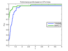
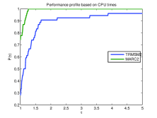
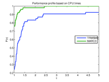
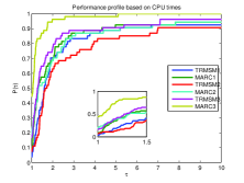
Figure 1: Performance profiles based on CPU time

For each problem, some more information are also given in Table 1, $r$ is the ratio of the cost time of computing the exact Hessians once and cost time of one function-gradient calculation, the 4th column Time gives the cost time of 20 function-gradient calculations. For different $r$, when the exact Hessian is used, the TRU and ARC method always need less iterations but more cost time than the TRMSM3 and MARC3 methods. Firstly, when $r$ is very large, such as 3641 for problem VARDIM, calculating the exact Hessians even once could cost much computing resource. On the other hand, even if $r$ is small, another inner iterative algorithm for solving trust region or cubic model subproblems is still needed and this step may cost much time. But for the TRMSM3 or MARC3 method, we only use the function value and the gradient information, and at each step, $O(n)$ operations are needed to form $\gamma_{k}$.

Next, we mainly compare MARC with TRMSM methods when employing different $\gamma_{k}$. We terminate the iteration when

$$\|g_{k}\|_{\infty}\leq 10^{-6}(1+|f(x_{k})|).$$

In addition, we also stop the algorithm if the number of iterations exceeds 5000. The detailed numerical results are given in Tables 2–3. Dolan and Moré’s [14] performance profiles are used to display the behaviors of these methods.

Figure 1 shows comparison of different methods based on cpu time. By using the same $\gamma_{k}$ parameter, the VMARC algorithm obviously outperform the TRMSM algorithm. Among these six methods, the MARC3 method has the best numerical performance, which can solve about 45% of the tested problems in the shortest time. Similar conclusions can be draw from Figure 2, which show the performance profiles based on iterations and function evaluations.

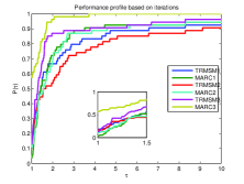
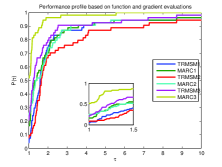
Figure 2: Performance profiles based on iterations and function evaluations

6 Conclusion

In this paper, combing with the Barzilai-Borwein step size, we present a modified adaptive cubic regularization method for large-scale unconstrained optimization problem. With nonmonotone technique, a variant of the modified method is also proposed. Convergence of the method is analyzed under some reasonable assumptions. Numerical experiments are performed to show the effectiveness of the new methods.

Table 1: Numerical comparisons between ARC/TR and TRMSM/MARC methods

Problem Dim $r$ Time ARC TRU TRMSM3 MARC3 iter cpu iter cpu iter ng cpu iter ng cpu POWER 5000 8328.6 2.67-03 26 27.497 33 32.747 55 125 0.023 92 170 0.032 VARDIM 2000 3641.1 1.59-03 27 6.873 719 182.221 52 157 0.015 5 36 0.003 BROWNAL 200 586.47 1.49-02 7 0.349 7 0.315 6 23 0.004 4 11 0.002 PENALTY1 1000 456.2 1.02-03 28 0.759 37 0.933 12 46 0.003 6 14 0.001 FMINSURF 1024 246.9 2.41-03 373 32.209 117 8.416 1172 1799 0.242 821 1548 0.202 SPARSQUR 5000 218.2 1.07-02 22 0.205 20 0.153 22 41 0.024 17 22 0.013 DQRTIC 2000 180.7 3.11-03 28 0.009 36 0.012 39 82 0.007 31 47 0.004 SROSENBR 5000 140.9 4.05-03 12 0.016 10 0.012 27 59 0.015 29 49 0.013 NONDIA 5000 102.1 5.61-03 29 0.033 24 0.03 4 25 0.008 5 14 0.004 WOODS 4000 87.8 4.23-03 56 0.062 67 0.077 195 329 0.089 453 860 0.224 DQDRTIC 5000 73.1 7.72-03 9 0.013 2 0.004 20 29 0.014 35 36 0.017 ARWHEAD 5000 70.5 8.26-03 10 0.015 6 0.009 13 29 0.013 14 21 0.01 ENGVAL1 5000 65.8 8.70-03 12 0.035 9 0.026 25 34 0.018 22 23 0.012 SINQUAD 5000 63.1 9.38-03 34 0.089 45 0.118 - - - 305 591 0.428 CRAGGLVY 5000 40.8 1.44-02 17 0.102 15 0.082 144 246 0.234 138 263 0.252 DIXMAANJ 3000 36.7 5.79-03 50 0.273 76 0.28 683 1075 0.355 444 839 0.277 DIXMAANJ 9000 275.1 1.72-02 68 1.086 80 0.873 531 840 0.826 410 776 0.752 DIXMAAND 3000 35.7 5.91-03 16 0.082 17 0.056 10 17 0.005 11 12 0.004 DIXMAAND 9000 108.3 1.74-02 17 0.326 43 0.275 9 16 0.016 12 13 0.014 MOREBV 5000 31.2 1.90-02 2 0.286 1 0.312 134 213 0.083 129 247 0.091 COSINE 2000 24.2 3.69-03 42 0.053 - - 11 13 0.004 15 17 0.005 EDENSCH 2000 21.3 4.42-03 17 0.027 16 0.024 27 36 0.009 29 30 0.008 BROYDN7D 5000 20.2 2.92-02 767 13.791 679 6.553 2325 3563 6.938 2039 3688 7.159 EXTROSNB 5000 13.3 1.01-03 685 16.134 703 1.788 35 45 0.015 76 143 0.045 EG2 1000 6.9 1.96-03 7 0.003 3 0.001 5 16 0.002 6 11 0.001 SENSORS 1000 1.7 5.24-00 683 316.162 33 36.078 42 66 22.958 29 33 9.99

Table 2: Numerical results of VMARC and TRMSM methods

Problem n TRMSM1 MARC1 TRMSM2 MARC2 TRMSM3 MARC3 iter nf cpu iter nf cpu iter nf cpu iter nf cpu iter nf cpu iter nf cpu ARWHEAD 10000 10 27 0.0250 10 18 0.0170 10 27 0.0264 9 17 0.0161 13 30 0.0285 12 20 0.0197 BDQRTIC 2000 3832 5964 1.3863 2469 4801 1.0979 3366 5242 1.1989 2188 4213 0.9635 1007 1584 0.3808 884 1691 0.4010 BOX 10000 3015 4689 6.1013 2009 3891 4.9861 2770 4305 5.5816 1793 3462 4.4329 698 1085 1.4385 668 1278 1.6854 BROWNAL 400 8 27 0.0200 10 17 0.0129 8 27 0.0198 10 17 0.0129 10 29 0.0212 12 19 0.0146 BROYDN7D 5000 2448 3752 7.1970 2178 3961 7.5734 2152 3272 6.2765 2195 3949 7.5585 2252 3455 6.6699 2007 3656 7.0330 BRYBND 10000 36 48 0.0695 39 44 0.0641 41 60 0.0862 47 56 0.0808 41 60 0.0877 37 42 0.0625 CHAINWOO 4000 2418 3739 1.6920 1781 3402 1.5169 2543 3923 1.7780 1901 3602 1.6060 - - - 714 1372 0.6252 CHNROSNB 50 4153 6365 0.0286 3289 6174 0.0269 4154 6387 0.0282 3199 5986 0.0272 2339 3626 0.0169 1592 3015 0.0134 COSINE 1000 8 10 0.0013 9 11 0.0014 7 9 0.0011 8 10 0.0012 8 10 0.0018 10 12 0.0016 CRAGGLVY 10000 131 230 0.4323 153 296 0.5551 593 935 1.7850 127 244 0.4611 151 261 0.4977 117 227 0.4377 CURLY10 5000 1201 1858 0.8318 945 1770 0.7834 1208 1860 0.8360 857 1622 0.7156 711 1096 0.5082 515 969 0.4398 DIXMAANA 9000 7 11 0.0111 10 11 0.0109 7 12 0.0112 9 10 0.0096 8 12 0.0119 10 11 0.0114 DIXMAANB 9000 7 12 0.0121 10 11 0.0109 8 14 0.0130 9 10 0.0098 8 13 0.0127 9 10 0.0104 DIXMAANC 9000 7 13 0.0126 12 13 0.0128 9 16 0.0150 11 12 0.0117 9 15 0.0146 12 13 0.0134 DIXMAAND 9000 8 15 0.0144 12 13 0.0128 11 19 0.0180 11 12 0.0120 10 17 0.0164 13 14 0.0144 DIXMAANE 9000 4155 6379 6.3765 3932 7401 6.9272 3855 5922 6.1231 3757 7040 6.5577 2448 3778 3.6779 1858 3517 3.3661 DIXMAANF 9000 4567 6988 7.1188 3718 6922 6.5570 4322 6629 6.5669 3434 6486 6.0325 2718 4203 4.0829 1387 2618 2.5130 DIXMAANG 9000 4504 6907 7.1448 3770 7073 6.5246 3715 5689 5.8587 3801 7159 6.8260 2527 3885 3.8372 1589 3019 2.8511 DIXMAANH 9000 4500 6904 7.6149 3414 6453 6.0810 3891 5982 6.5304 3560 6701 6.4195 1993 3094 3.0510 1564 2989 2.8864 DIXMAANJ 9000 1925 2966 3.0635 1343 2548 2.3553 1685 2604 2.5713 1461 2752 2.5503 1244 1928 1.8484 780 1470 1.3879 DIXMAANL 9000 1053 1633 1.5780 817 1560 1.4602 1100 1726 1.6520 940 1771 1.6585 757 1188 1.1570 482 908 0.8718 DQDRTIC 10000 27 36 0.0324 36 37 0.0339 27 36 0.0319 36 37 0.0338 24 33 0.0304 32 33 0.0317 DQRTIC 2000 55 90 0.0078 51 65 0.0059 45 79 0.0068 41 51 0.0046 58 101 0.0092 58 85 0.0080 EDENSCH 5000 21 30 0.0197 19 25 0.0156 18 31 0.0191 23 28 0.0174 19 28 0.0186 29 38 0.0243 EG2 1000 3 14 0.0017 4 9 0.0011 3 14 0.0016 4 9 0.0010 4 15 0.0017 5 10 0.0012 ENGVAL1 10000 14 23 0.0219 17 18 0.0178 10 18 0.0170 17 18 0.0179 16 25 0.0246 17 18 0.0187 EXTROSNB 5000 69 101 0.0314 52 54 0.0176 - - - 91 172 0.0510 45 55 0.0186 77 144 0.0452

Table 3: Numerical results of VMARC and TRMSM methods (Continued)

Problem n TRMSM1 MARC1 TRMSM2 MARC2 TRMSM3 MARC3 iter nf cpu iter nf cpu iter nf cpu iter nf cpu iter nf cpu iter nf cpu FMINSURF 5625 - - - 4877 9110 6.6111 - - - 4299 8054 5.7941 3324 5094 3.7929 2540 4745 3.4735 FLETCBV3 10000 9 10 0.0166 10 11 0.0172 9 10 0.0163 11 12 0.0188 9 10 0.0171 10 11 0.0177 FREUROTH 5000 1195 1849 1.1744 943 1768 1.1088 465 735 0.4651 289 554 0.3447 282 452 0.2908 51 105 0.0665 HILBERTA 50 3257 4964 0.2494 2214 4156 0.2076 3253 4970 0.2476 2274 4211 0.2110 1247 1923 0.0968 496 941 0.0479 HILBERTB 50 8 12 0.0007 8 9 0.0005 8 12 0.0007 8 9 0.0005 8 12 0.0007 8 9 0.0005 GENROSE 500 - - - 4960 9190 0.3893 - - - - - - 3969 6062 0.2706 3625 6721 0.2996 INDEF 5000 - - - - - - - - - - - - - - - 3179 5816 3.4597 LIARWHD 1000 2950 4619 0.3932 1744 3393 0.2869 2935 4581 0.4010 1644 3223 0.2738 905 1433 0.1316 624 1195 0.1044 MOREBV 5000 174 269 0.0985 156 301 0.1079 197 309 0.1126 157 302 0.1073 134 213 0.0810 129 247 0.0912 NCB20 1010 1526 2326 3.5559 1626 3038 4.6309 1688 2591 3.9688 1725 3190 4.8743 926 1442 2.2099 868 1634 2.5030 NCB20B 2000 90 162 0.5026 62 125 0.3866 74 137 0.4245 64 130 0.4018 58 102 0.3162 65 128 0.3975 NONDIA 5000 25 64 0.0208 26 53 0.0176 26 65 0.0211 38 80 0.0264 20 55 0.0181 21 45 0.0153 PENALTY1 1000 50 84 0.0053 123 234 0.0140 96 153 0.0092 35 43 0.0028 132 251 0.0152 130 239 0.0144 POWER 5000 2268 3520 0.6415 1761 3278 0.5582 2587 3974 0.7455 1990 3717 0.6410 1468 2301 0.4365 1283 2367 0.4311 POWELLSG 1000 - - - - - - - - - - - - - - - 603 1147 0.0521 QUARTC 1000 46 73 0.0033 40 44 0.0022 48 83 0.0036 36 46 0.0021 50 83 0.0038 31 35 0.0018 SCHMVETT 5000 20 23 0.0313 37 38 0.0507 54 94 0.1237 35 42 0.0562 30 58 0.0766 39 40 0.0545 SENSORS 1000 30 39 15.1534 22 26 8.1429 23 31 9.6644 20 24 6.1264 31 55 16.9737 24 28 7.2498 SINQUAD 10000 32 44 0.0637 23 40 0.0566 19 33 0.0469 18 24 0.0344 29 46 0.0677 25 41 0.0604 SPARSQUR 5000 29 44 0.0261 29 34 0.0200 26 46 0.0265 26 34 0.0196 39 70 0.0407 23 28 0.0172 SROSENBR 5000 21 39 0.0100 18 28 0.0071 16 33 0.0084 21 35 0.0091 28 60 0.0152 33 53 0.0140 TOINTGOR 50 191 308 0.0032 171 327 0.0033 201 324 0.0032 160 306 0.0031 134 227 0.0024 132 253 0.0026 TOINTPSP 50 212 344 0.0016 252 481 0.0020 238 381 0.0015 231 441 0.0017 142 232 0.0010 181 343 0.0014 TOINTQOR 50 44 59 0.0002 42 46 0.0002 44 59 0.0002 42 46 0.0002 37 42 0.0002 36 37 0.0001 VARDIM 5000 369 639 0.1533 345 636 0.1499 369 639 0.1518 346 640 0.1500 369 639 0.1608 339 636 0.1575 VAREIGVL 50 28 32 0.0003 27 28 0.0002 118 204 0.0016 104 202 0.0015 28 32 0.0003 27 28 0.0002 WOODS 10000 84 156 0.0972 799 1534 0.9510 1590 2475 1.5742 1147 2171 1.3462 481 773 0.5111 72 107 0.0720

References

- [1] J. Barzilai and J. Borwein, Two-point step size gradient methods, IMA J. Numer. Anal. 8 (1988), pp. 141–148.
- [2] H.Y. Benson and D.F. Shanno, Cubic regularization in symmetric rank-1 quasi-Newton methods, Math. Program. Comput. 10 (2018), pp. 457–486.
- [3] E. Bergou, Y. Diouane, and S. Gratton, On the use of the energy norm in trust-region and adaptive cubic regularization subproblems, Comput. Optim. Appl. 68 (2017), pp. 533–554.
- [4] T. Bianconcini and M. Sciandrone, A cubic regularization algorithm for unconstrained optimization using line search and nonmonotone techniques, Optim. Methods Softw. 31 (2016), pp. 1008–1035.
- [5] T. Bianconcini, G. Liuzzi, B. Morini, and M. Sciandrone, On the use of iterative methods in cubic regularization for unconstrained optimization, Comput. Optim. Appl. 60 (2015), pp. 35–57.
- [6] E.G. Birgin, J.L. Gardenghi, J.M. Martínez, S.A. Santos, and P.L. Toint, Worst-case evaluation complexity for unconstrained nonlinear optimization using high-order regularized models, Math. Program. 163 (2017), pp. 359–368.
- [7] C. Cartis, N. Gould, and P. Toint, Worst-case evaluation complexity of regularization methods for smooth unconstrained optimization using Hölder continuous gradients, Optim. Methods Softw. 32 (2017), pp. 1273–1298.
- [8] C. Cartis, N.I.M. Gould, and P.L. Toint, Adaptive cubic regularisation methods for unconstrained optimization. Part I: motivation, convergence and numerical results, Math. Program. 127 (2011), pp. 245–295.
- [9] C. Cartis, N.I.M. Gould, and P.L. Toint, Adaptive cubic regularisation methods for unconstrained optimization. Part II: worst-case function- and derivative-evaluation complexity, Math. Program. 130 (2011), pp. 295–319.
- [10] A.R. Conn, N.I. Gould, and P.L. Toint, Trust-Region Methods (MPS-SIAM Series on Optimization), SIAM, Philadelphia, 2000.
- [11] Y.H. Dai and R. Fletcher, Projected Barzilai-Borwein methods for large-scale box-constrained quadratic programming, Numer. Math. 100 (2005), pp. 21–47.
- [12] Y.H. Dai and C.X. Kou, A nonlinear conjugate gradient algorithm with an optimal property and an improved Wolfe line search, SIAM J. Optim. 23 (2013), pp. 296–320.
- [13] N. Deng, Y. Xiao, and F. Zhou, Nonmonotonic trust region algorithm, J. Optim. Theory Appl. 76 (1993), pp. 259–285.
- [14] E.D. Dolan and J.J. Moré, Benchmarking optimization software with performance profiles, Math. Program. 91 (2002), pp. 201–213.
- [15] J.P. Dussault, ARC q : a new adaptive regularization by cubics, Optim. Methods Softw. 33 (2018), pp. 322–335.
- [16] N.I.M. Gould, D. Orban, and P.L. Toint, GALAHAD, a library of thread-safe Fortran 90 packages for large-scale nonlinear optimization, ACM Trans. Math. Softw. 29 (2003), pp. 353–372.
- [17] N.I.M. Gould, D. Orban, and P.L. Toint, CUTEst: a Constrained and Unconstrained Testing Environment with safe threads for mathematical optimization, Comput. Optim. Appl. 60 (2015), pp. 545–557.
- [18] N.I.M. Gould, M. Porcelli, and P.L. Toint, Updating the regularization parameter in the adaptive cubic regularization algorithm, Comput. Optim. Appl. 53 (2012), pp. 1–22.
- [19] L. Grippo, F. Lampariello, and S. Lucidi., A nonmonotone line search technique for Newton’s method, SIAM J. Numer. Anal. 23 (1986), pp. 707–716.
- [20] Y. Huang, H. Liu, and S. Zhou, An efficient monotone projected Barzilai-Borwein method for nonnegative matrix factorization, Appl. Math. Lett. 45 (2015), pp. 12–17.
- [21] J.M. Martínez, On High-order Model Regularization for Constrained Optimization, SIAM J. Optim. 27 (2017), pp. 2447–2458.
- [22] J.M. Martínez and M. Raydan, Cubic-regularization counterpart of a variable-norm trust-region method for unconstrained minimization, J. Glob. Optim. 68 (2017), pp. 367–385.
- [23] V. Morovati, L. Pourkarimi, and H. Basirzadeh, Barzilai and Borwein’s method for multiobjective optimization problems, Numer. Algorithms 72 (2016), pp. 539–604.
- [24] J. Nocedal and S.J. Wright, Numerical Optimization, Springer, New York, 2006.
- [25] M. Raydan, The Barzilai and Borwein gradient method for the large scale unconstrained minimization problem, SIAM J. Optim. 7 (1997), pp. 26–33.
- [26] W. Sun, Nonmonotone trust region method for solving optimization problems, Appl. Math. Comput. 156 (2004), pp. 159–174.
- [27] H. Yabe, H. Ogasawara, and M. Yoshino, Local and superlinear convergence of quasi-Newton methods based on modified secant conditions, J. Comput. Appl. Math. 205 (2007), pp. 617–632.
- [28] H. Zhang and W.W. Hager, A nonmonotone line search technique and its application to unconstrained optimization, SIAM J. Optim. 14 (2004), pp. 1043–1056.
- [29] Y. Zheng and B. Zheng, A New Modified Barzilai–Borwein Gradient Method for the Quadratic Minimization Problem, J. Optim. Theory Appl. 172 (2017), pp. 179–186.
- [30] Q. Zhou and D. Hang, Nonmonotone adaptive trust region method with line search based on new diagonal updating, Appl. Numer. Math. 91 (2015), pp. 75–88.
- [31] Q. Zhou, W. Sun, and H. Zhang, A new simple model trust-region method with generalized Barzilai-Borwein parameter for large-scale optimization, Sci. China Math. 59 (2016), pp. 2265–2280.