Complex trainable ISTA for linear and nonlinear inverse problems

Abstract

Complex-field signal recovery problems from noisy linear/nonlinear measurements appear in many areas of signal processing and wireless communications. In this paper, we propose a trainable iterative signal recovery algorithm named complex-field TISTA (C-TISTA) which treats complex-field nonlinear inverse problems. C-TISTA is based on the concept of deep unfolding and consists of a gradient descent step with the Wirtinger derivatives followed by a shrinkage step with a trainable complex-valued shrinkage function. Importantly, it contains a small number of trainable parameters so that its training process can be executed efficiently. Numerical results indicate that C-TISTA shows remarkable signal recovery performance compared with existing algorithms.

Index Terms—  deep learning, deep unfolding, Wirtinger derivative, compressed sensing, amplitude clipping

1 Introduction

Inverse problems are prevalent topics in signal processing and wireless communications. For example, linear inverse problems consider estimating inputs $\bm{x}\in\mathbb{R}^{n}$ from noisy observations $\bm{y}=\bm{A}\bm{x}+\bm{w}\in\mathbb{R}^{m}$ and can model, for example, signal detection in multiple access systems with a channel matrix $\bm{A}$ such as multiple-input multiple-output (MIMO) and orthogonal frequency-division multiplexing (OFDM) systems [1]. In these cases, we have prior information that the inputs take discrete values defined by a signal constellation. Compressed sensing (CS) [2, 3, 4] is another popular class of inverse problems widely applied to wireless communication techniques [5]. CS enables recovery of sparse signals accurately even in underdetermined cases, i.e., $m<n$, which is the case, e.g. in overloaded non-orthogonal multiple-access systems.

Recently machine learning methods have been shown to be a powerful tool for inverse problems in wireless communications [6]. In particular, deep unfolding which originated in learned iterative soft thresholding algorithm (LISTA) [7] is a promising technique to derive tailored deep networks due to its high scalability and ability to use prior information efficiently [8]. Deep unfolding is based on starting with iterative algorithms and then unrolling their recursive structures to deep networks with trainable parameters. These parameters are trained by supervised signals using deep learning techniques. A number of deep unfolding-based algorithms have been proposed: learned approximate message passing (LAMP) [9] and trainable ISTA (TISTA) for CS [10], MIMO detectors [11, 12], OFDM signal detectors [13], trainable robust principle component analysis [14], and decoders for error-correcting codes [15, 16]. They are mainly based on signal recovery algorithms for real-valued linear systems.

A drawback of these algorithms is a limitation to complex-field nonlinear inverse problems with nonlinear observations $\bm{y}=f(\bm{A}\bm{x})+\bm{w}$, where $f:\mathbb{C}\rightarrow\mathbb{C}$ is an element-wise function. For complex-valued problems, a conventional transformation from complex vectors to real vectors is typically used. However, it possibly breaks correlations between real and imaginary parts of signals, which can degrade signal recovery performance. Adaptability to nonlinearity is another crucial issue. Amplitude clipping and quantization are important in nonlinear CS [17]. In wireless communications, amplitude clipping arises in OFDM systems to reduce peak power [18], and quantization corresponds to the use of analog-to-digital converters.

In this paper, we propose a trainable signal recovery algorithm to treat complex-field nonlinear inverse problems in a direct and general manner by deep unfolding. The algorithm named complex-field TISTA (C-TISTA) is constructed as an extension of TISTA using the Wirtinger derivative and complex-valued shrinkage function with trainable parameters. Numerical simulations demonstrate that C-TISTA outperforms existing algorithms in complex-valued CS and clipped OFDM signal detection.

Throughout the paper, we use the following notation: For a function $f:\mathbb{C}\rightarrow\mathbb{C}$ and $\bm{v}=(v_{1},\dots,v_{n})^{T}\in\mathbb{C}^{n}$, we define $f(\bm{v}):=(f(v_{1}),\dots,f(v_{n}))^{T}$. For a vector $\bm{z}$, $\bm{z}^{\ast}$ represents its conjugate. For a matrix $\bm{A}:=(A_{i,j})\in\mathbb{C}^{m\times n}$, $\bm{A}^{H}:=(A_{j,i}^{\ast})$ is its Hermitian transpose. We define $\mathcal{CN}(\mu,\sigma^{2})$ as a complex Gaussian distribution with mean $\mu$ and variance $\sigma^{2}$. The p.d.f. of $\mathcal{CN}(\mu,\sigma^{2})$ is defined by

$$G(x;\mu,\sigma^{2}):=\frac{1}{\pi\sigma^{2}}\exp\left(-\frac{|x-\mu|^{2}}{\sigma^{2}}\right).$$ (1)

For a random variable $\bm{x}\in\mathbb{C}^{n}$ and a function $g:\mathbb{C}^{n}\rightarrow\mathbb{C}^{n}$, $\mathsf{E}_{\bm{x}}g(\bm{x})$ denotes the expectation of $g(\bm{x})$ with respect to $\bm{x}$.

2 Brief review of TISTA

We first briefly review TISTA for real-valued linear observations defined by

$$\bm{y}=\bm{A}\bm{x}+\bm{w},$$ (2)

where $\bm{A}\in\mathbb{R}^{m\times n}(n\geq m)$ and $\bm{x}\in\mathbb{R}^{n}$. Each entry of the noise vector $\bm{w}\in\mathbb{R}^{m}$ follows a zero-mean Gaussian distribution with variance $\sigma^{2}$. We also assume that the prior information on $\bm{x}$ is known.

For a sparse input $\bm{x}$, LASSO formulation [19] is conventionally used for its estimation, leading to

$$\bm{\hat{x}}=\mathrm{minimize}_{\bm{x}\in\mathbb{R}^{n}}\|\bm{y}-\bm{A}\bm{x}\|_{2}^{2}+\lambda\|\bm{x}\|_{1},$$ (3)

where $\|\cdot\|_{1}$ is the $\ell_{1}$ norm and $\lambda$ is a positive constant.

ISTA [20] is a simple iterative algorithm to solve (3). It consists of the following recursions:

$$\bm{s}^{(t+1)}:=\eta_{s}(\bm{s}^{(t)}+\beta\bm{A}^{T}(\bm{y}-\bm{A}\bm{s}^{(t)});\tau),$$ (4)

where $\beta(>0)$ is a step size and $\eta_{s}(r;\tau)={\sf sign}(r)\max\{|r|-\tau,0\}$ is the element-wise soft thresholding function with threshold $\tau\in\mathbb{R}$ $(\tau>0)$ related to $\lambda$. Since the soft thresholding function is the proximal operator of the $\ell_{1}$-regularizer, ISTA can be seen as a proximal gradient descent algorithm for solving (3). Note that, in order to have convergence, the step size $\beta$ should be carefully chosen [20].

LISTA [7] is a trainable algorithm based on ISTA. As deep unfolding, the signal-flow graph of ISTA is expanded to a deep network with embedded trainable parameters such as a step size. The recursive formula is given by

$$\bm{s}^{(t+1)}:=\eta_{s}(\bm{B}_{t}\bm{y}+\bm{C}_{t}\bm{s}^{(t)};\tau_{t}),$$ (5)

where $\{\bm{B}_{t},\bm{C}_{t},\tau_{t}\}_{t=1}^{T}$ is a set of trainable parameters. These parameters are learned by back propagation and stochastic gradient descent using training data. Although the convergence speed of LISTA is significantly faster than that of ISTA, its training process is costly and sometimes unstable because the number of trainable parameters is large, i.e., $(mn+n^{2}+1)T$ in $T$ iterations.

TISTA [10] is another trainable algorithm for the system (2), which is based on orthogonal AMP [21] and defined by

$$\bm{r}^{(t)} :=\bm{s}^{(t)}+\gamma_{t}\bm{W}(\bm{y}-\bm{A}\bm{s}^{(t)}),$$ (6)

$$\bm{s}^{(t+1)} :=\eta_{m}(\bm{r}^{(t)};\tau_{t}^{2}),$$ (7)

$$v_{t}^{2} :=\max\left\{\frac{\|\bm{y}-\bm{A}\bm{s}^{(t)}\|_{2}^{2}-m\sigma^{2}}{{\sf tr}(\bm{A}^{T}\bm{A})},\epsilon\right\},$$ (8)

$$\tau_{t}^{2} :=\frac{v_{t}^{2}}{n}(n+(\gamma^{2}_{t}-2\gamma_{t})m)+\frac{\gamma_{t}^{2}\sigma^{2}}{n}{\sf tr}(\bm{W}\bm{W}^{T}),$$ (9)

where the matrix $\bm{W}\!=\!\bm{A}^{T}(\bm{A}\bm{A}^{T})^{-1}$ is the pseudo-inverse matrix of $\bm{A}$. The shrinkage function $\eta_{m}(\cdot)$ is an element-wise minimum mean square error (MMSE) shrinkage function whose shape is similar to the soft shrinkage function. The parameter $\gamma_{t}$ is a trainable parameter that can be optimized in training process. TISTA has only $T$ trainable parameters in $T$ iterations. This fact leads to scalable and stable training process compared with LISTA. In addition, TISTA can improve signal recovery performance and adaptability to wide range of measurement matrices in CS [10].

In this paper, we propose a TISTA-based algorithm for complex-field nonlinear systems. We will modify (6)-(9) using the Wirtinger derivative and a trainable shrinkage function corresponding to various prior information including sparsity and discreteness.

3 Complex-field TISTA

3.1 System Model

We consider a complex-field nonlinear system given by

$$\bm{y}=f(\bm{A}\bm{x})+\bm{w},$$ (10)

where $\bm{A}\in\mathbb{C}^{m\times n}$ is a measurement matrix. The vector $\bm{x}\in\mathbb{C}^{n}$ is the input vector on which a certain prior information such as sparsity or discreteness is imposed. Each component of the the noise vector $\bm{w}\in\mathbb{C}^{m}$ follows ${\cal CN}(0,\sigma^{2})$. The inverse problem is the estimation the input from the observation $\bm{y}$ based on $\bm{A}$ and $f$.

3.2 Complex-field TISTA

We now propose C-TISTA for complex-field nonlinear inverse problems. We apply the Wirtinger derivative and trainable complex-valued shrinkage function to TISTA. The recursive formulas of C-TISTA are given as follows:

$$\bm{r}^{(t)} :=\bm{s}^{(t)}+\beta_{t}h(\bm{s}^{(t)}),$$ (11)

$$\bm{s}^{(t+1)} :=C_{t}(\eta(\bm{r}^{(t)};\lambda^{(t)})-D_{t}\bm{r}_{t}),$$ (12)

$$h(\bm{s}) :=\bm{V}\left[\{\bm{y}-f(\bm{A}\bm{s})\}^{\ast}\odot\frac{\partial f}{\partial z^{\ast}}(\bm{A}\bm{s})\right.$$

$$\left.\qquad\qquad\quad+\{\bm{y}-f(\bm{A}\bm{s})\}\odot\frac{\partial f^{\ast}}{\partial z^{\ast}}(\bm{A}\bm{s})\right],$$ (13)

where $\eta(z;\lambda):\mathbb{C}\rightarrow\mathbb{C}$ is a nonlinear function with a parameter $\lambda$ and $\odot$ is the Hadamard product. The definition of the Wirtinger derivative and derivation of (13) can be found in Appendix A. As a matrix $\bm{V}$, we can use $\bm{A}^{{H}}$ or the pseudo-inverse matrix $\bm{W}:=(\bm{A}^{H}\bm{A})^{-1}\bm{A}^{H}$ ($m\leq n$) similar to TISTA. Starting from an initial point $\bm{s}^{(1)}$, the estimate after $T$ iterations is given by $\bm{\hat{x}}:=\bm{s}^{(T+1)}$. The trainable parameters of C-TISTA are $4T$ real scalars $\{\beta_{t},\lambda_{t},C_{t},D_{t}\}_{t=1}^{T}$, which is constant to $n$ and $m$ and leads to scalable and stable training process.

The first update rule (11) is a gradient step using the Wirtinger derivative whose step size is a trainable parameter $\beta_{t}(>0)$. In the second update rule (12) called a shrinkage step, an estimate is updated by a trainable divergence free (DF)-like function [21, 22] with shrinkage function $\eta(\cdot)$ to reflect prior information on $\bm{x}$ and trainable parameters $\{\lambda_{t},C_{t},D_{t}\}$.

In this paper, we use two shrinkage functions depending on prior information. The first one is the complex-valued soft shrinkage function for sparse prior. It is defined by

$$\eta_{{cs}}(x;\lambda):=\eta_{s}(x;\lambda)e^{\mathrm{j}\varphi(x)},$$ (14)

where $\varphi(x)$ is the phase of $x$ and $\lambda(>0)$ means the threshold [23]. The second one is an MMSE estimator for discrete signals. Let $x$ be a random variable uniformly chosen from a signal constellation $S:=\{s_{1},s_{2},\ldots,s_{M}\}\subset\mathbb{C}$ of size $M$. For a virtual AWGN channel $p(y|x)=G(y;x,\lambda)$ with variance $\lambda$, the MMSE function is given by

$$\eta(y;\lambda):={\sf E}_{{x}}[x|y]=\frac{\sum_{s\in S}s\exp\left(-\frac{|y-s|^{2}}{\lambda}\right)}{\sum_{s\in S}\exp\left(-\frac{|y-s|^{2}}{\lambda}\right)}.$$ (15)

4 Numerical Results

We here examine the recovery performance of C-TISTA in complex-valued CS and clipped OFDM signal detection.

4.1 Implementation Details

C-TISTA is implemented by PyTorch 1.2 [24]. We set an initial point to $\bm{s}^{(1)}\!=\!\bm{W}\bm{y}$ and use the pseudo-inverse matrix $\bm{W}$ as $\bm{V}$ in (13). The training parameter $\lambda_{t}$ is replaced by $a_{t}^{2}$ to satisfy the identity $\lambda_{t}\!>\!0$. Training process is executed by incremental training similar to TISTA [10] to avoid a vanishing-gradient problem. Adam optimizer [25] with learning rate $0.005$ is used to minimize the MSE loss function between the true signal $\bm{x}$ and estimate $\bm{\hat{x}}$. The parameters are initialized as $(\beta_{t},a_{t},C_{t},D_{t})=(0.1,1,1,0)$ for $t=1,\dots,T$.

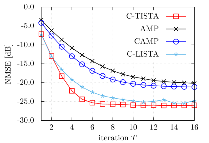
Fig. 1: Signal recovery in complex-valued CS ($n\!=\!240$, $m\!=\!120$, $p\!=\!0.1$). NMSEs are plotted as functions of iteration $T$. Symbols represent C-TISTA (squares), AMP (cross marks), CAMP (circles), and C-LISTA (asterisks).

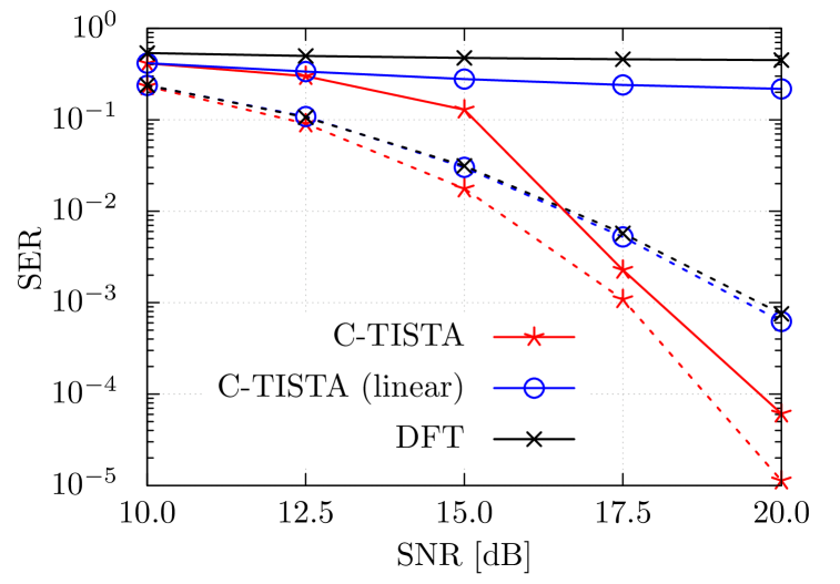
(a) SER as a function of SNR.

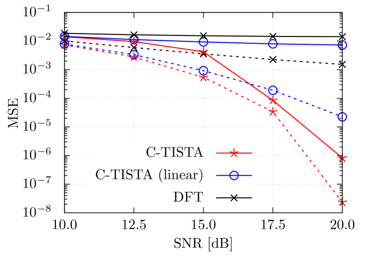
(b) MSE as a function of SNR.

Fig. 2: Signal detection in clipped OFDM systems ($n=192$). Symbols represent C-TISTA (stars), C-TISTA without nonlinearity (C-TISTA (linear); circles), and DFT (cross marks) and lines represent PAPR$=1.5$dB (solid) and $5$dB (broken).

4.2 Complex-Valued Compressed Sensing

We first consider complex-field CS related to spectrum sensing [26] and angle-of-arrival detection [27].

We consider an underdetermined linear system $\bm{y}=\bm{A}\bm{x}+\bm{w}$ of size $(n,m)=(240,120)$. As sparse prior, we assume that each element of $\bm{x}$ follows the complex Gaussian-Bernoulli prior $p(x)=(1-p)\delta(x)+pG(x;0,\sigma_{\mathrm{x}}^{2})$ with $p=0.1$ and $\sigma_{\mathrm{x}}^{2}=1.0$. This means that there are around 10% non-zero elements in $\bm{x}$. Each component of $\bm{A}$ follows ${\cal CN}(0,1/{m})$ and the noise variance of $\bm{w}$ is $\sigma^{2}=0.03^{2}$.

The soft thresholding function $\eta_{cs}(\cdot)$ is used in C-TISTA. The number of mini-batches is $K=2000$ and the batch size is $L=200$ in its training process.

As baselines, we perform AMP [28] and complex AMP (CAMP) [23]. Complex numbers are transformed to real numbers to execute AMP. In addition, complex-field LISTA (C-LISTA) is also executed for comparison. It is defined by

$$\bm{s}^{(t+1)}:=\eta_{cs}(\bm{B}\bm{y}+\bm{C}\bm{s}^{(t)};\tau_{t}),$$ (16)

with trainable parameters $\bm{B}\in\mathbb{C}^{n\times m}$, $\bm{C}\in\mathbb{C}^{n\times n}$, and $\tau_{t}\in\mathbb{R}$ ($t=1,\dots,T$). For stable training and reasonable performance, trainable parameters are are shared with all iterations, i.e., $\bm{B}$ and $\bm{C}$ unlike the real-valued case (5).

Figure 1 shows normalized MSE (NMSE) performance as a function of the number of iterations $T$. It is found that the NMSE of C-TISTA decreases most rapidly. C-TISTA reaches to NMSE$=$$-25$dB at $T=6$ and almost converges to $-26$dB at $T=8$. AMP and CAMP show slower convergence reaching to around $-20$dB and $-21$dB at $T=15$, respectively. Neglecting correlations of complex vectors by a complex-to-real transformation in AMP degrades signal recovery performance. Although C-LISTA shows better NMSE performance than AMP and CAMP, C-TISTA outperforms C-LISTA in terms of convergence speed and convergent NMSE (about $-25$dB by C-LISTA) with faster training process. This is because C-TISTA is more flexible thanks to trainable step sizes $\{\beta_{t}\}_{t=1}^{T}$ and a tunable DF-like function. It is emphasized that C-TISTA has only $4T$ trainable parameters while C-LISTA has $n^{2}+nm+T$ parameters in total. These results show that C-TISTA successfully recovers complex-valued sparse signals with fast convergence and improved accuracy.

4.3 16-QAM Signal Detection in Clipped OFDM Systems

We next examine a clipped OFDM system as a nonlinear system with discrete inputs. Amplitude clipping limits peaks of a time-domain signal containing the sum of contributions from multiple carriers. It reduces the peak-to-average power ratio (PAPR) with low complexity [18] and is useful to avoid signal saturation at an amplifier. However, it causes signal distortion that degrades performance of the zero-forcing detector by the discrete Fourier transformation (DFT).

The clipped OFDM system is formulated as the nonlinear system $\bm{y}\!=\!f_{c}(\bm{F}\bm{x})\!+\!\bm{w}$ of $n$ carriers. We assume that each signal $x_{i}$ is uniformly chosen from 16-QAM signal points, i.e., $x_{i}\!=\!p\!+\!\mathrm{j}q$ ($p,q\!\in\!\{\pm 1,\pm 3\}$). The matrix $\bm{F}$ is the $n\times n$ inverse DFT matrix whose $(l,m)$-element is given by $\exp\left(\mathrm{j}{2\pi lm}/{n}\right)/{\sqrt{n}}$. The function $f_{c}(z)$ is a clipping function defined by

$$f_{c}(z):=\begin{cases}z&(|z|\leq\alpha)\\ \alpha e^{\mathrm{j}\varphi(z)}&(|z|>\alpha)\end{cases}.$$ (17)

The clipping level $\alpha(>0)$ is defined as the PAPR given by $10\log_{10}({\max_{1\leq k\leq n}|\tilde{x}_{k}|^{2}}/{\mathsf{E}_{\bm{x}}\|\bm{Fx}\|_{2}^{2}})$, where $\bm{\tilde{x}}\!:=\!f_{c}(\bm{Fx})$. Small PAPR indicates large distortion. Here, we set $n\!=\!128$ and PAPR$=\!1.5$dB or $5$dB as strongly clipped systems.

As a shrinkage function of C-TISTA, we use the MMSE function (15) based on the uniform distribution over the 16-QAM constellation. In addition to C-TISTA, we also perform C-TISTA without nonlinearity to study influence of nonlinearlity. C-TISTA without nonlinearity named C-TISTA (linear) has a gradient corresponding to $f_{c}(z)=z$. In the training process, we set $K=500$, $L=200$, and $T=10$.

Figure 2 (a) shows the symbol error ratio (SER) performance as a function of the signal-to-noise ratio (SNR). The results show that SERs of DFT and C-TISTA (linear) are largely affected by the value of PAPR. In contrast, C-TISTA shows nearly the same SER performance even when the clipping level is small. It suggests that the signal distortion introduced by amplitude clipping is correctly compensated by C-TISTA. In fact, compared with DFT and C-TISTA (linear), C-TISTA exhibits better detection performance: the gain of C-TISTA is about $2$dB when SER$=\!1.0\times 10^{-3}$ and PAPR$=$5dB, which becomes much larger when PAPR$=1.5$dB.

MSE performance is also important if a belief propagation decoder for LDPC codes is applied to the system to deal with in-band distortion [29]. Fig. 2 (b) shows the SNR dependency of the MSE performance in the same setting. The result shows that C-TISTA also detects transmitted signals with high accuracy. These results suggest that C-TISTA can detect a discrete signal even in nonlinear inverse problems.

5 Conclusion

In this paper, we propose C-TISTA for complex-field nonlinear inverse problems that have wide applications such as complex-valued CS and signal detection from nonlinear measurements. C-TISTA consists of a gradient step with Wirtinger derivatives followed by a shrinkage step with a trainable complex shrinkage function. Its training is scalable and stable because it has a small number of trainable parameters. Numerical studies reveal that C-TISTA shows remarkable signal recovery performance in complex-valued CS and clipped OFDM systems. These results indicate a promising potential of C-TISTA for wide range of inverse problems in signal processing and wireless communications.

Appendix A Gradient Descent by the Wirtinger Derivative

In this Appendix, we briefly review Wirtinger derivative and derive a gradient descent method for solving the least mean square (LMS) problem for (10), i.e.,

$$\mathrm{Minimize}_{\bm{x}\in\mathbb{C}^{n}}g(\bm{x}):=\frac{1}{2}\|\bm{y}-f(\bm{A}\bm{x})\|_{2}^{2},$$ (18)

without prior information.

A simple extension of the gradient descent method for a real-valued problem is not applicable to the complex-valued problem (18) because the function $g(\bm{x})$ does not have complex differentiability. To overcome this difficulty, we here use Wirtinger derivative in complex analysis as an extension of partial derivative with respect to real variables. For a function $f:\mathbb{C}\rightarrow\mathbb{C}$ and ${z}:={z}_{\mathrm{r}}+\mathrm{j}{z}_{\mathrm{i}}\in\mathbb{C}$ (${z}_{\mathrm{r}}=\mathrm{Re}(z),{z}_{\mathrm{i}}=\mathrm{Im}(z)$), we introduce a function $F:\mathbb{R}^{2}\rightarrow\mathbb{C}$ such that $F({z}_{\mathrm{r}},{z}_{\mathrm{i}})=f(z)$. Wirtinger derivative is then defined by

$$\frac{\partial f(z)}{\partial z} :=\frac{1}{2}\left[\frac{\partial}{\partial{z}_{\mathrm{r}}}-\mathrm{j}\frac{\partial}{\partial{z}_{\mathrm{i}}}\right]F({z}_{\mathrm{r}},{z}_{\mathrm{i}}),$$ (19)

$$\frac{\partial f(z)}{\partial z^{\ast}} :=\frac{1}{2}\left[\frac{\partial}{\partial{z}_{\mathrm{r}}}+\mathrm{j}\frac{\partial}{\partial{z}_{\mathrm{i}}}\right]F({z}_{\mathrm{r}},{z}_{\mathrm{i}}),$$ (20)

by using partial derivatives [30]. For a complex vector $\bm{z}\in\mathbb{C}^{n}$, we define differential operators $\frac{\partial}{\partial\bm{z}}:=\left(\frac{\partial}{\partial z_{1}},\dots,\frac{\partial}{\partial z_{n}}\right)^{\mathrm{T}}$, and $\frac{\partial}{\partial\bm{z}^{\ast}}:=\left(\frac{\partial}{\partial z_{1}^{\ast}},\dots,\frac{\partial}{\partial z_{n}^{\ast}}\right)^{\mathrm{T}}$. It is known that the steepest descent direction is given by $-\partial f/\partial\bm{z}^{\ast}$ [31], not $-\partial f/\partial\bm{z}$. We thus calculate $\nabla g(\bm{x}):=-\partial g/\partial\bm{x}^{\ast}$ of (18) to solve the LMS problem by gradient descent.

We first calculate the Wirtinger derivative with respect to the first variable $x_{1}^{\ast}$ based on the assumption that the function $f$ is applied to a vector component-wisely. We have

$$\frac{\partial}{\partial x_{1}^{\ast}}g(\bm{x})= -\frac{1}{2}\sum_{i=1}^{m}\left[\{y_{i}-f(\bm{A}_{i,:}\bm{x})\}^{\ast}\frac{\partial}{\partial x_{1}^{\ast}}\left(f(\bm{A}_{i,:}\bm{x})\right)\right.$$

$$\left.\qquad\qquad+\{y_{i}-f(\bm{a}_{i,:}\bm{x})\}\frac{\partial}{\partial x_{1}^{\ast}}\left(f^{\ast}(\bm{A}_{i,:}\bm{x})\right)\right]$$

$$= -\frac{1}{2}\sum_{i=1}^{m}A_{i1}^{\ast}\left[\{y_{i}-f(\bm{A}_{i,:}\bm{x})\}^{\ast}\frac{\partial f}{\partial z^{\ast}}(\bm{A}_{i,:}\bm{x})\right.$$

$$\left.\qquad\qquad\quad+\{y_{i}-f(\bm{A}_{i,:}\bm{x})\}\frac{\partial f^{\ast}}{\partial z^{\ast}}(\bm{A}_{i,:}\bm{x})\right],$$ (21)

where $\bm{A}_{i,:}:=(A_{i1},\dots,A_{in})$ ($1\leq i\leq m$) of the matrix $\bm{A}$ and $\frac{\partial f}{\partial z^{\ast}}\left(\bm{u}\right):=\left.\frac{\partial f(z)}{\partial z^{\ast}}\right|_{z=\bm{u}}$. We use a chain rule [30], i.e.,

$$\frac{\partial}{\partial z^{\ast}}(f_{1}\circ f_{2})=\left(\frac{\partial f_{1}}{\partial z}\circ f_{2}\right)\frac{\partial f_{2}}{\partial z^{\ast}}+\left(\frac{\partial f_{1}}{\partial z^{\ast}}\circ f_{2}\right)\frac{\partial f_{2}^{\ast}}{\partial z^{\ast}},$$ (22)

for functions $f_{1},f_{2}:\mathbb{C}\rightarrow\mathbb{C}$, and an identity $\partial z/\partial z^{\ast}=\partial z^{\ast}/\partial z=0$ in the second line of (21).

Combining it with derivatives with respect to other variables, we finally obtain

$$\nabla g(\bm{x}) =-\frac{1}{2}\bm{A}^{H}\left[\{\bm{y}-f(\bm{A}\bm{x})\}^{\ast}\odot\frac{\partial f}{\partial z^{\ast}}(\bm{A}\bm{x})\right.$$

$$\left.\qquad\qquad\quad+\{\bm{y}-f(\bm{A}\bm{x})\}\odot\frac{\partial f^{\ast}}{\partial z^{\ast}}(\bm{A}\bm{x})\right],$$ (23)

where $\frac{\partial f}{\partial z^{\ast}}\left(\bm{u}\right):=\left.\frac{\partial f(z)}{\partial z^{\ast}}\right|_{z=\bm{u}}$. It corresponds to (13) in the gradient step of C-TISTA when $\bm{V}=\bm{A}^{H}$.

Based on the gradient (23), the update rule of the gradient descent method is given by

$$\bm{x}^{(t+1)}=\bm{x}^{(t)}-2\beta\nabla g(\bm{x}^{(t)})$$ (24)

with a step-size parameter $\beta(>0)$ and an initial value $\bm{x}^{(1)}$. The factor $2$ in (24) is necessary to keep consistency with the real-valued case.

It would be useful to simplify (23) for several special cases. For a linear model in which $f(z)=z$, we have

$$\nabla g(\bm{x})=-\frac{1}{2}\bm{A}^{H}(\bm{y}-\bm{A}\bm{x}).$$ (25)

This corresponds to the gradient descent step in ISTA (4) for real-valued linear systems.

If $f(z)$ is an analytic function, we have

$$\nabla g(\bm{x})=-\frac{1}{2}\bm{A}^{H}\left[\{\bm{y}-f(\bm{A}\bm{x})\}\odot f^{\prime}(\bm{A}\bm{x})\right],$$ (26)

where $f^{\prime}(z)$ is a complex derivative with respect to $z$. Similarly, for a real-valued system in which $\bm{A}\in\mathbb{R}^{m\times n}$, $\bm{x},\bm{w}\in\mathbb{R}^{n}$, and $f:\mathbb{R}\rightarrow\mathbb{R}$, we obtain

$$\nabla g(\bm{x})=-\frac{1}{2}\bm{A}^{T}\left[\{\bm{y}-f(\bm{A}\bm{x})\}\odot f^{\prime}(\bm{A}\bm{x})\right].$$ (27)

References

- [1] D. Tse and P. Viswanath, Fundamentals of Wireless Communication. Cambridge University Press, 2005.
- [2] D. L. Donoho, “Compressed Sensing,” IEEE Trans. Info. Theory, vol. 52, no. 4, pp. 1289–1306, Apr. 2006.
- [3] Y. C. Eldar and G. Kutyniok, Compressed Sensing: Theory and Applications. Cambridge University Press, 2012.
- [4] Y. C. Eldar, Sampling Theory: Beyond Bandlimited Systems. Cambridge University Press, 2015.
- [5] K. Hayashi, M. Nagahara, and T. Tanaka, “A user’s Guide to Compressed Sensing for Communications Systems”, IEICE Trans. Comm., vol. E96.B, pp. 685–712, Mar., 2013.
- [6] C. Jiang, H. Zhang, Y. Ren, Z. Han, K. Chen and L. Hanzo, “Machine Learning Paradigms for Next-Generation Wireless Networks,” IEEE Wireless Comm., vol. 24, no. 2, pp. 98-105, Apr. 2017.
- [7] K. Gregor and Y. LeCun, “Learning Fast Approximations of Sparse Coding,” Proc. 27th Int. Conf. Machine Learning, pp. 399–406, 2010.
- [8] A. Balatsoukas-Stimming and C. Studer, “Deep Unfolding for Communications Systems: A Survey and Some New Directions,” arXiv:1906.05774, 2019.
- [9] M. Borgerding, P. Schniter, and S. Rangan, ”AMP-Inspired Deep Networks for Sparse Linear Inverse Problems,” IEEE Trans. Signal Proc., vol. 65, no. 16, pp. 4293-4308, Aug.15, 2017.
- [10] D. Ito, S. Takabe, and T. Wadayama, “Trainable ISTA for Sparse Signal Recovery,” IEEE Trans. Signal Proc., vol. 67, no. 12, pp. 3113-3125, Jun., 2019.
- [11] N. Samuel, T. Diskin, and A. Wiesel, “Deep MIMO Detection,” 2017 IEEE 18th Int. Workshop Signal Process. Advances in Wireless Comm., Jul. 2017, pp. 1-5.
- [12] S. Takabe, M. Imanishi, T. Wadayama, R. Hayakawa and K. Hayashi, “Trainable Projected Gradient Detector for Massive Overloaded MIMO Channels: Data-Driven Tuning Approach,” IEEE Access, vol. 7, pp. 93326-93338, 2019.
- [13] J. Zhang, H. He, C. Wen, S. Jin, and G. Y. Li, ”Deep Learning Based on Orthogonal Approximate Message Passing for CP-Free OFDM,” 2019 IEEE Int. Conf. Acoustics, Speech, Signal Process. (ICASSP), Brighton, United Kingdom, 2019, pp. 8414-8418.
- [14] O. Solomon et al., “Deep Unfolded Robust PCA with Application to Clutter Suppression in Ultrasound,” to appear in IEEE Trans. Med. Imaging, 2019.
- [15] E. Nachmani, Y. Beéry and D. Burshtein, “Learning to Decode Linear Codes Using Deep Learning,” 2016 54th Ann. Allerton Conf. Comm., Control, Comp., Monticello, IL, 2016, pp. 341-346.
- [16] T. Wadayama and S. Takabe, “Deep Learning-Aided Trainable Projected Gradient Decoding for LDPC Codes,” IEEE Int. Symp. Info. Theory (ISIT), 2019.
- [17] Z. Yang, Z. Wang, H. Liu, Y. C. Eldar, T. Zhang, “Sparse Nonlinear Regression: Parameter Estimation under Nonconvexity,” 33rd Int. Conf. Machine Learning (ICML), vol. 48, pp. 2472-2481, 2016.
- [18] H. Han and J. H. Lee, “An Overview of Peak-to-Average Power Ratio Reduction Techniques for Multicarrier Transmission,” IEEE Wireless Commun. Mag., Vol. 12, No. 2, pp. 56–65, April 2005.
- [19] R. Tibshirani, “Regression Shrinkage and Selection via the Lasso,” J. Royal Stat. Society, Series B, vol. 58, pp. 267–288, 1996.
- [20] A. Chambolle, R. A. DeVore, N. Lee, and B. J. Lucier, “Nonlinear Wavelet Image Processing: Variational Problems, Compression, and Noise Removal Through Wavelet Shrinkage,” IEEE Trans. Image Process., vol. 7, no. 3, pp. 319–335, Mar, 1998.
- [21] J. Ma and L. Ping, “Orthogonal AMP,” IEEE Access, vol. 5, pp. 2020-2033, Jan. 2017.
- [22] H. He, C. Wen, S. Jin, and G. Y. Li, ”Model-Driven Deep Learning for Joint MIMO Channel Estimation and Signal Detection,” arXiv:1907.09439, 2019.
- [23] A. Maleki, L. Anitori, Z. Yang, and R. G. Baraniuk, “Asymptotic Analysis of Complex LASSO via Complex Approximate Message Passing (CAMP),” IEEE Trans. Info. Theory, vol. 59, no. 7, pp. 4290–4308, July 2013.
- [24] A. Paszke et al., “Automatic Differentiation in PyTorch,” 31st Conf. Neural Inf. Process. Syst., pp. 1–4, 2017; https://pytorch.org
- [25] D. P. Kingma and J. L. Ba, “Adam: A Method for Stochastic Optimization,” arXiv:1412.6980, 2014.
- [26] Z. Tian and G. B. Giannakis, “Compressed Sensing for Wideband Cognitive Radios,” 2007 IEEE Int. Conf. Acoustics, Speech and Sig. Proc. (ICCASP), Honolulu, HI, April 2007, pp. IV-1357–IV-1360.
- [27] A. C. Gurbuz, J. H. McClellan, and V. Cevher, “A Compressive Beamforming Method,” 2008 IEEE Int. Conf. Acoustics, Speech and Sig. Proc. (ICCASP), Las Vegas, NV, 2008, pp. 2617–2620.
- [28] D. L. Donoho, A. Maleki, and A. Montanari, “Message Passing Algorithms for Compressed Sensing,” Proc. Natl. Acad. Sci., vol. 106, pp. 18914–18919, 2009.
- [29] R. D. Soriano and J. S. Marciano, “The Effect of Signal Distortion Techniques for PAPR Reduction on the BER Performance of LDPC and Turbo Coded OFDM System,” 2006 IEEE Region 10 Conf., Hong Kong, pp. 1-4, 2006.
- [30] R. Remmert, Theory of Complex Functions. Harrisonburg, VA: Springer-Verlag, 1991.
- [31] B. Widrow, J. McCool, and M. Ball, “The Complex LMS Algorithm,” Proc. IEEE, vol. 63, no. 4, pp. 719-720, April 1975.