Dynamical phase behavior of the single- and multi-lane asymmetric simple exclusion process via matrix product states

Abstract

We analyze the dynamical phases of the current-biased 1D and multi-lane open asymmetric simple exclusion processes (ASEP), using matrix product states and the density matrix renormalization group (DMRG) algorithm. In the 1D ASEP, we present a systematic numerical study of the current cumulant generating function and its derivatives, which serve as dynamical phase order parameters. We further characterize the microscopic structure of the phases from local observables and the entanglement spectrum. In the multi-lane ASEP, which may be viewed as finite width 2D strip, we use the same approach and find the longitudinal current-biased dynamical phase behavior to be sensitive to transverse boundary conditions. Our results serve to illustrate the potential of tensor networks in the simulation of classical nonequilibrium statistical models.

I Introduction

Connecting microscopic states to macroscopic properties is a central goal of statistical mechanics. At equilibrium, this connection is expressed through the Gibbs-Boltzmann framework, which defines the free energy and its derivatives in terms of microscopic states. Large deviation theory (LDT) provides an analogous framework for nonequilibrium systems. Large deviation functions (LDFs), such as the cumulant generating function (CGF) $\psi$, and the rate function $\phi$, are analogs of the equilibrium free energy and entropy. Their derivatives provide information on dynamical order parameters and rare fluctuations as a system is driven away from equilibrium  Donsker and Varadhan (1975); Ellis (1985); Touchette (2009).

For LDT to be applied to practical problems requires the development of robust numerical tools to compute LDFs. Monte Carlo sampling methods, such as the cloning algorithm and transition path sampling Lasanta, A. et al. (2016); Nemoto et al. (2017); Ray et al. (2018a) augmented with importance sampling Nemoto et al. (2016); Klymko et al. (2018); Ray et al. (2018b) as well as recent direct rate function evaluation techniques Jacobson and Whitelam (2019) have been applied to lattice and continuum nonequilibrium systems Derrida et al. (2003); Bodineau and Derrida (2005); Garrahan et al. (2009); de Gier and Essler (2011); Gorissen and Vanderzande (2011); Gorissen et al. (2012); Prados et al. (2012); Lasanta, A. et al. (2016); Carollo et al. (2018); Ray et al. (2018a); Brewer et al. (2018); Schile and Limmer (2018); GrandPre and Limmer (2018); Gao and Limmer (2018). Alternatively, tensor network (TN) methods provide analytic or numerical representations of the steady state of a master equation, with some common examples being the matrix ansatz Derrida et al. (1993); Blythe and Evans (2007) and the density matrix renormalization group (DMRG) algorithm  Carlon et al. (1999); Gorissen et al. (2009, 2012); Gorissen and Vanderzande (2011); Johnson et al. (2010). Recently, the TN approach has been applied to kinetically constrained models of glasses Bañuls and Garrahan (2019).

In this report, we compute the current cumulant generating function and other properties of the dynamical phases of the 1D (single-lane) and multi-lane asymmetric simple exclusion process (ASEP), under open boundary conditions, using matrix product states (MPS) and the DMRG. In 1D, the ASEP is a paradigmatic model of nonequilibrium statistical mechanics that can be solved semi-analytically with the matrix ansatz and functional Bethe ansatz and has been studied via many numerical approaches Derrida and Lebowitz (1998); Prolhac (2009); Lazarescu (2015); Lazarescu and Pasquier (2014), though detailing the microscopic structure in all regions of the phase diagram remains challenging. While DMRG has previously been used to compute high-order current cumulants of the 1D ASEP to verify analytic expressions Gorissen et al. (2012), a systematic application across the phase diagram of this model has yet to be presented. Thus we start with a short benchmarking study of the 1D ASEP using the DMRG, focusing on the phases induced by a current bias and the associated macro and microscopic behaviors. We then examine the phase behavior of the multi-lane version of the ASEP under a longitudinal current bias for systems with up to 4 lanes. The multi-lane model can be thought of as a finite-width version of the 2D ASEP and it is the first time, to our knowledge, that this family of models has been studied.

II Large Deviation Theory and Matrix Product States

We first briefly summarize some relevant concepts in large deviation theory, the theory of matrix product states and the density matrix renormalization group. A more complete description can be found in recent reviews Touchette (2009, 2011); Ray et al. (2018a); Schollwöck (2011).

In a nonequilibrium system, the state vector $|P_{t}\rangle$ evolves from an initial state $|P_{0}\rangle$ according to a master equation with dynamics generated by a non-Hermitian Markov operator $\mathcal{W}$,

$$\partial_{t}|P_{t}\rangle=\mathcal{W}|P_{t}\rangle,$$ (1)

with the probability of a system configuration $\mathcal{C}$ at time $t$ given by $\text{Prob}(\mathcal{C}_{t})\equiv\langle\mathcal{C}|P_{t}\rangle$. The long-time limit yields the final (steady) state $|P_{\infty}\rangle$. The probability of observing a given trajectory of configurations $\mathscr{C}(t_{N})=\{\mathcal{C}_{0},\mathcal{C}_{1},\dots,\mathcal{C}_{t_{N}}\}$ at times $\{t_{0},\cdots,t_{N}\}$ ($dt=t_{N}/N$) is,

$$\text{Prob}(\mathscr{C}(t_{N}))=\text{Prob}(\mathcal{C}_{0})\prod_{i=0}^{t_{N-1}}\langle\mathcal{C}_{i+1}|e^{dt\mathcal{W}}|\mathcal{C}_{i}\rangle.$$ (2)

We can define dynamical observables along such a trajectory, such as a time-local observable ${\mathcal{O}}=\sum_{i=0}^{t_{N-1}}o(\mathcal{C}_{i+1},\mathcal{C}_{i})$, with $o$ being an arbitrary function of time-adjacent configurations ($\mathcal{C}_{i+1}$ and $\mathcal{C}_{i}$). To characterize the steady-state expectation value and fluctuations of this observable, we define a cumulant generating function, $\psi(\lambda)$,

$$\psi(\lambda) =\lim_{t_{N}\rightarrow\infty}\ln\left<e^{-\lambda\mathcal{O}}\right>$$

$$=\lim_{t_{N}\rightarrow\infty}\ln\sum_{\mathscr{C}(t_{N})}\text{Prob}(\mathscr{C}(t_{N}))e^{-\lambda\mathcal{O}},$$ (3)

where $\lambda$ is a field conjugate to the observable. At $\lambda=0$, the first derivative of $\psi$ is the observable’s steady-state expectation value $\langle o\rangle$; characterizations of the fluctuations of $o$, via its cumulants, are obtained from higher-order derivatives of $\psi$. A fundamental result in LDT is that $\psi(\lambda)$ is the largest eigenvalue of a tilted operator $\mathcal{W}_{\lambda}$, i.e.,

$$\mathcal{W}_{\lambda}|P^{\lambda}\rangle=\psi(\lambda)|P^{\lambda}\rangle,$$ (4)

where, for discrete configurations,

$$\mathcal{W}_{\lambda}(\mathcal{C},\mathcal{C}^{\prime})=\mathcal{W}(\mathcal{C},\mathcal{C}^{\prime})e^{-\lambda o(\mathcal{C},\mathcal{C}^{\prime})}(1-\delta_{\mathcal{C},\mathcal{C}^{\prime}})-R(\mathcal{C})\delta_{\mathcal{C},\mathcal{C}^{\prime}}$$ (5)

with $R(\mathcal{C})=\sum_{\mathcal{C}\neq\mathcal{C}^{\prime}}\mathcal{W}(\mathcal{C},\mathcal{C}^{\prime})$. Furthermore, the corresponding right (left) eigenvector $|P^{\lambda}\rangle$ ($\langle P^{\lambda}|$) gives the probability of a configuration in the final (initial) state conditioned on trajectories satisfying $\langle o\rangle=d\psi(\lambda)/d\lambda$ Lebowitz and Spohn (1999).

The computation of $\psi(\lambda)$ from the eigenvalue problem in Eq. (4) can be recast as a generalized variational problem,

$$\langle\delta P^{\lambda}|\mathcal{W}_{\lambda}|P^{\lambda}\rangle-\psi(\lambda)\langle\delta P^{\lambda}|P^{\lambda}\rangle=0.$$ (6)

Because $\mathcal{W}_{\lambda}$ is non-Hermitian, for an approximate $|P^{\lambda}\rangle$, $\langle P^{\lambda}|$, $\langle P^{\lambda}|\mathcal{W}_{\lambda}|P^{\lambda}\rangle$ may be above or below the exact $\psi(\lambda)$.

In this work, we use an MPS as an ansatz for $|P^{\lambda}\rangle$ and perform the optimization in Eq. (6) using the DMRG algorithm for non-Hermitian operators Carlon et al. (1999); Chan and Van Voorhis (2005). For a lattice of length $L$, a configuration $\mathcal{C}$ is an ordered list of the local states $\sigma_{i}$ of sites $i=1\ldots L$,

$$|\mathcal{C}\rangle=\ket{\sigma_{1},\cdots,\sigma_{L}}$$ (7)

An MPS expresses the configurational probability $\text{Prob}(\mathcal{C})$ as a matrix product

$$\text{Prob}(\mathcal{C})=\bm{M}^{\sigma_{1}}\bm{M}^{\sigma_{2}}\cdots\bm{M}^{\sigma_{L-1}}\bm{M}^{\sigma_{L}}$$ (8)

where the matrices $\bm{M}^{\sigma_{i}}$ ($i=2\ldots L-1$) are of dimension $D\times D$, and the first and last matrices are of dimension $1\times D$ and $D\times 1$ respectively. The bond dimension $D$ controls the accuracy of the ansatz and may be increased until the ansatz is exact. The matrix product contains a local gauge (i.e. $\{\bm{M}^{\sigma_{i}}\}$ can be varied while keeping the matrix product invariant) which can be fixed by choosing a canonical form,

$$\text{Prob}(\mathcal{C})=\bm{L}^{\sigma_{1}}\bm{L}^{\sigma_{2}}\cdots\bm{F}^{\sigma_{i}}\cdots\bm{R}^{\sigma_{L-1}}\bm{R}^{\sigma_{L}},$$ (9)

where $\sum_{\sigma}{\bm{L}^{\sigma}}^{\dagger}\bm{L}^{\sigma}=\bm{I}$ and $\sum_{\sigma}\bm{R}^{\sigma}{\bm{R}^{\sigma}}^{\dagger}=\bm{I}$.

The canonical form of Eq. (9) also simplifies the computation of the bipartite entanglement entropy $S(i)$ at site $i$, a quantification of the non-factorizable correlations between the states of sites to the left and right of site $i$. By reshaping the central rank-3 tensor into a matrix, with $\bm{G}_{\sigma_{i}p,q}=\bm{F}^{\sigma_{i}}_{pq}$, $S(i)$ is conveniently computed as,

$$S(i)=-\sum_{m}s_{m}^{2}\log_{2}s_{m}^{2},$$ (10)

where {$s_{m}$} are the singular values of $\bm{G}$.

Figure 1: A diagrammatic representation of the mapping of a 2D lattice with nearest neighbor interactions onto a 1D lattice with long range interactions. The arrows indicate how our DMRG optimization traverses the 2D lattice and the dashed line shows the bond over which the reported entanglement entropy is measured.

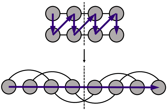
Because the MPS representation of a state requires a 1D site ordering, associated with the sequence of matrices in Eq. (8), we must define a 1D traversal pattern for the multi-lane ASEP. We do so using a zig-zag ordering of sites, shown in Fig. 1. Note that for fixed accuracy, the bond dimension of the matrices in the MPS usually needs to increase exponentially with the number of lanes studied, reflecting independent fluctuations in the different lanes.

III Model

Figure 2: The ASEP model where particles on a 1D lattice stochastically hop to a vacant neighboring right (left) site at a rate of $p$ ($q$) and enter (exit) at the left and right boundaries at rates $\alpha$ ($\gamma$) and $\beta$ ($\delta$).

The 1D Simple Exclusion Process (SEP) (Fig. 2) takes place on a 1D lattice of $L$ sites. Particles hop stochastically to vacant nearest-neighbor sites at the following rates. In the lattice interior, particles hop right (left) with rate $p$ ($q$) with asymmetry enforced via $p\neq q$ (ASEP). At the edges, particles enter (exit) at the left with rate $\alpha$ ($\gamma$) and at the right with rate $\beta$ ($\delta$). In this work we focus on phases induced by the current bias $\lambda$ in the parameter regime $\alpha=\beta=\gamma=\delta=1/2$ and $p+q=1$. The tilted operator for the current cumulant generating function is,

$$\mathcal{W}^{\text{1D}}_{\lambda}= \alpha\left(e^{\lambda}\bm{a}_{1}^{\dagger}-\bm{v}_{1}\right)+\gamma\left(e^{-\lambda}\bm{a}_{1}-\bm{n}_{1}\right)$$ (11)

$$+\sum_{i=1}^{L-1}p\left(e^{\lambda}\bm{a}_{i}\bm{a}_{i+1}^{\dagger}-\bm{n}_{i}\bm{v}_{i+1}\right)$$

$$+\sum_{i=1}^{L-1}q\left(e^{-\lambda}\bm{a}_{i}^{\dagger}\bm{a}_{i+1}-\bm{v}_{i}\bm{n}_{i+1}\right)$$

$$+\beta\left(e^{-\lambda}\bm{a}_{L}^{\dagger}-\bm{v}_{L}\right)+\delta\left(e^{\lambda}\bm{a}_{L}-\bm{n}_{L}\right),$$

where $\bm{a}_{i}$, $\bm{a}_{i}^{\dagger}$, $\bm{n}_{i}$ and $\bm{v}_{i}$ are annihilation, creation, particle number, and vacancy number operators. Note that the tilted operator is invariant with respect to the combined operation of particle-hole transformation/inversion ($\bm{a}^{\dagger}\leftrightarrow\bm{a}$ and $\{...,i,i+1,...\}\leftrightarrow\{...,i+1,i,...\}$). The eigenvalues of $\mathcal{W}^{\text{1D}}_{\lambda}$ also exhibit a Gallavotti-Cohen (GC) symmetry Gallavotti and Cohen (1995); Lebowitz and Spohn (1999) of the form $\psi(\lambda)=\psi(\lambda^{*})$ where, for the specified ASEP parameters, $\lambda^{*}=-\frac{L-1}{L+1}\ln(p/q)-\lambda$.

The multi-lane ASEP is defined on a 2D lattice of $L_{y}\times L_{x}$ sites. It augments the 1D ASEP with bulk hopping in the vertical (transverse) direction (at rates $p_{y}$, $q_{y}$) and particles inserted and removed at the vertical boundaries (at rates $\alpha_{y},\beta_{y},\gamma_{y},\delta_{y}$). We apply the current bias in the (longitudinal) $x$-direction, with a tilted operator that takes the form,

$$\mathcal{W}^{\mathrm{2D}}_{\lambda}=\mathcal{W}^{\mathrm{1D_{x}}}_{\lambda}+\mathcal{W}^{\mathrm{1D_{y}}}_{0},$$ (12)

and retains the above GC and particle-hole/inversion symmetries. To understand the effects of the transverse parameters on the longitudinal system’s phase behavior, we focus on two multi-lane parameter sets, namely open and closed vertical boundaries. Both require $p_{x}+q_{x}=1$, $p_{y}=q_{y}=1/2$, and $\alpha_{x}=\beta_{x}=\gamma_{x}=\delta_{x}=1/2$, while the open (closed) case specifies $\alpha_{y}=\beta_{y}=\gamma_{y}=\delta_{y}=1/2$ ($\alpha_{y}=\beta_{y}=\gamma_{y}=\delta_{y}=0$).

To characterize the system, the DMRG algorithm is used to determine the largest eigenvalue of each tilted operator, through which the steady-state total current and current susceptibility are computed as $J=\partial\psi(\lambda)/d\lambda$ and $\chi=\partial^{2}\psi(\lambda)/d\lambda^{2}$. Local densities, currents, and activities may also be computed by contracting the resulting left and right eigenvector with the appropriate operator, i.e.,

$$\rho_{i} =\bra{P^{\lambda}}\bm{n}_{i}\ket{P^{\lambda}},$$ (13)

$$J_{i} =\bra{P^{\lambda}}pe^{\lambda}\bm{a}_{i}\bm{a}_{i+1}^{\dagger}-qe^{-\lambda}\bm{a}_{i}^{\dagger}\bm{a}_{i+1}\ket{P^{\lambda}},$$

$$K_{i} =\bra{P^{\lambda}}pe^{\lambda}\bm{a}_{i}\bm{a}_{i+1}^{\dagger}+qe^{-\lambda}\bm{a}_{i}^{\dagger}\bm{a}_{i+1}\ket{P^{\lambda}},$$

assuming $\bra{P^{\lambda}}\ket{P^{\lambda}}=1$.

IV Results

Figure 3: (a) Rudimentary sketches of the density profiles in the three possible phases. Blue curves represent approximate steady-state density profiles while green curves depict typical particle configurations. (b) A map of the dynamical phase behavior of the ASEP showing the steady-state current $J$ as a function of $p$ and $\lambda$ for a length $L=20$ lattice as determined via DMRG. Additionally shown in black are lines indicating the center of the GC symmetry (solid) and the predicted boundaries between the MC and shock phases (dotted, via macroscopic fluctuation theory Bertini et al. (2002, 2015); Lazarescu (2015)) and the shock and HD+LD phases (dashed, via functional Bethe ansatz Prolhac and Mallick (2008); Lazarescu (2015)).

IV.1 Benchmark MPS calculations of the 1D ASEP

Figure 4: The behavior of the 1D ASEP with lattice lengths of $L=[10,100]$. The DMRG results for the normalized (a) CGF $\overline{\psi}=E_{0}/L$, (b), current $\overline{J}=\partial_{\lambda}\psi/L$, and (e) current susceptibility $\overline{\chi}=\partial_{\lambda}\psi/L^{2}$ compared with the analytic functional Bethe ansatz expressions (red), valid for $\lambda\to 0^{-}$ and $\lambda>0$; additionally (f) shows the gap between the ground and first excited state energies. Plots (c) and (d) show the density $\rho$ and recurrent hopping $K-|J|$ as a function of position in a $L=10$ lattice, $x$, and $\lambda$. (g) shows the entanglement entropy $S$ of a bipartition at the center bond as a function of $\lambda$ with the upper (lower) subfigures in (h) showing the corresponding ordered entanglement spectrum, with $\hat{S}_{m}=-s_{m}^{2}\log_{2}s_{m}^{2}$, at $\lambda=-0.3$ ($\lambda=0.3$).

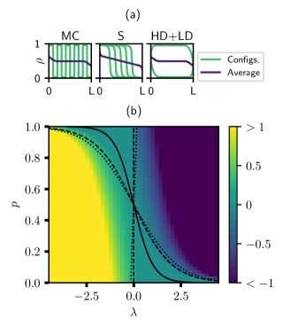
We begin by using MPS and DMRG to characterize the phase behavior in the aforementioned parameter space and benchmark this approach against earlier results from the semi-analytical functional Bethe ansatz and the approximate macroscopic fluctuation theory Lazarescu (2015). In this space, there are three expected phases, which are described in Fig. 3(a) via rudimentary sketches of both the steady-state density profile and the most probable particle configurations. These are the Maximal Current (MC) phase, where, in the most probable microscopic configurations, particles are evenly spaced throughout the lattice, allowing a maximal amount of biased hopping, the Shock (S) phase, where particles conglomerate on one side of the lattice to form a shock that, in path-space simulations, performs a Brownian walk on the lattice, and the High-Density/Low-Density Coexistence (HD+LD) phase, where the entirely filled and empty states (with some boundary effects) are degenerate in the thermodynamic limit and correspond to a steady-state density profile of $\rho=1/2$.

The predicted phase diagram is mapped in Fig. 3(b) where the lines indicate the line of GC symmetry (solid), the boundary between the MC and S phases (dotted, via macroscopic fluctuation theory), and the boundary between the S and HD+LD phases (dashed, via functional Bethe ansatz). The steady-state current is also shown, computed via DMRG for an $L=20$ ASEP, showing that current functions as a dynamical order parameter for the transition from S to HD+LD, going effectively to zero in the HD+LD phase. While the boundary between the MC and S phases is commonly defined as the point where the per site current is $J=1/4$, we are not aware of an order parameter for this transition, which instead appears as a smooth crossover in the current rather than a true phase boundary. Also note that because of the symmetries of the system, the remaining analysis can be limited to the lower left region of the parameter space ($p<1/2$ to the left of the line of GC symmetry), with the rest of the diagram mapped out by symmetry.

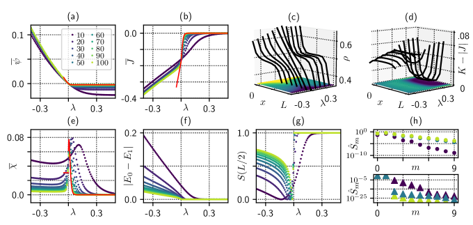
Finite size errors can be converged rapidly by increasing the lattice size. In Fig. 4, we characterize this behavior using system properties such as the cumulant generating function, current, current susceptibility, and excited state gap for a range of $\lambda$ near $\lambda=0$ with $p=0.1$ and for lattice sizes up to $L=100$ via DMRG with bond dimension $D$ between $50$ and $300$. As a benchmark, the solid red line in Fig. 4 (a), (b), and (e) corresponds to the functional Bethe ansatz results, which is valid only in the HD+LD phase and near $\lambda=0$ in the S phase.

As $L\to\infty$, a number of interesting behaviors are observed, particularly at the interface between the S and HD+LD phases. In this region, the cumulant generating function transitions from having a finite negative slope to become nearly flat, signifying a transition to a low current regime. We also see that the system becomes gapless here due to the degeneracy of the high-density and low-density configurations. Because the two degenerate states are of the same particle-hole/inversion symmetry while $\partial_{\lambda}\mathcal{W}_{\lambda}$ is odd under this symmetry, the closing gap does not contribute to the spike in the current susceptibility.

The MPS representation also provides the state’s full configurational information, enabling us to study the microscopic structure of the phases and quantities that are not derivatives of the cumulant generating function. Fig. 4 (c) and (d) show the steady-state density, $\rho$, and recurrent hopping, $K-|J|$, computed as specified in Eq. (13), as a function of the position in the lattice $x$ and the current bias $\lambda$. These density profiles correspond to those shown in Fig. 3(a), with the linear profile near $\lambda=0$ corresponding to the shock phase. The HD+LD and MC phases can here be distinguished via the rate of recurrent hopping; particles and holes are spatially dispersed in the MC phase, allowing frequent opportunities to hop back and forth, as indicated by the finite observed recurrent hopping at $\lambda<0$. When the transition is made into the HD+LD phase, the recurrent hopping drops to nearly zero in the lattice bulk, attributable to the lattice being nearly entirely filled or empty in this phase and thus providing few opportunities for recurrent hops.

An additional way to summarize the microscopic information (and the associated correlations in the system) is via the entanglement entropy and entanglement spectrum ($S(i)$ and $\{s_{m}\}$ in Eq. (10)) which we measure at the middle of the lattice. These are plotted for the right eigenvector $|P^{\lambda}\rangle$ in Fig. 4 (g). The entanglement spectrum provides details on the maximum bond dimension required to accurately represent a state and can be used as a generalized order parameter Kitaev and Preskill (2006); Pollmann et al. (2010). There are two clear regions present in the entanglement entropy, one corresponding to the MC phase, the other to the HD+LD phase. For the MC phase, the spectrum decays slowly, indicating that a relatively large bond dimension is required to accurately represent the given state. In the HD+LD phase, the entanglement entropy is larger and appears to be exactly $1$ ($\log_{2}2$). The entanglement spectrum shows that only two modes contribute, arising from the filled and empty configurations, indicating the state can be represented exactly by an MPS of bond dimension $2$. It is evident that the entanglement entropy converges as a function of $L$, indicating an area law.

IV.2 Multi-lane ASEP model

We now consider a system comprised of multiple ASEP lanes, with particles that may hop vertically ($y$-direction) or horizontally ($x$-direction), where we will examine the unexplored interplay between vertical and horizontal currents that can generate new phase behaviour.

IV.2.1 Closed Multi-lane ASEP

Figure 5: The behavior of the closed multi-lane ASEP showing the DMRG results for the normalized (a) CGF $\overline{\psi}=E_{0}/(L_{x}L_{y})$, (b) current $\overline{J}=\partial_{\lambda}\psi/(L_{x}L_{y})$, and (e) current susceptibility $\overline{\chi}=\partial_{\lambda}^{2}\psi/(L_{x}^{2}L_{y})$ as well as (f) the gap between the ground and first excited state energies for the four lane systems with lengths up to $L_{x}=50$. Plots (c) and (d) show the density $\rho$ and vertical hopping activity $K_{y}$ between lanes for a two-lane ASEP with $L_{x}=20$. (g) Shows the entanglement entropy $S$ of a bipartition of the system at the center bond as a function of $\lambda$.

Figure 6: Representations of the measured microscopic observables for a lattice of size $2\times 20$ for systems with both closed vertical boundary conditions, in (a) the MC phase ($\lambda=-0.3$) and (c) the HD+LD phase ($\lambda=0.3$), and open vertical boundary conditions, in (b) the MC phase ($\lambda=-0.3$) and (d) the HD+LD phase ($\lambda=0.3$). The grayscale shading of lattice sites indicates the measured steady-state density $\rho$ while the color of the arrows corresponds to the steady-state number of hops $K$ in the given direction. Only the five edge sites on each side are included because the behavior in the lattice bulk resembles what is seen at the center-most included sites.

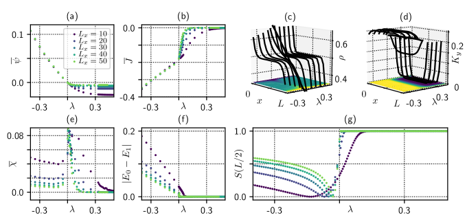
A simple, but nontrivial, extension of the 1D ASEP into multiple lanes, as specified in Sec. III, is to augment horizontal hopping and entry/exit parameters with equal vertical hopping rates $p_{y}=q_{y}=1/2$ and no entry/exit at the vertical bounds, i.e. closed boundary conditions. To understand the phase behavior here, we again carried out DMRG calculations mapping out the behavior as a function of the longitudinal current bias $\lambda_{x}$ for fixed $p_{x}=0.1$, with bond dimensions $D$ between $50$ and $300$ and with system widths and lengths of up to $L_{y}=4$ and $L_{x}=50$.

The resulting cumulant generating function, current, current susceptibility, and first excited state gap are displayed respectively in Fig. 5 (a), (b), (d) and (e) for the $L_{y}=4$ ASEP (with the $L_{y}=[2,3]$ results being essentially indistinguishable from these). A comparison between this figure and Fig. 4 shows no qualitative difference between the single lane and closed multi-lane ASEP. We can analyze the ground state MPS to confirm whether the microscopic configurations in the multi-lane system correspond to those seen in 1D.

Fig. 5 (c) and (d) show the behaviors of key observables as a function of $\lambda$ while Fig. 6 (a) and (c) compare snapshots of microscopic observable behaviors when the system is respectively in the MC and HD+LD phases. Using results from a two lane calculation, Fig. 5 (c) shows the density profile in one of the lanes as a function of $\lambda$, with the most notable point being the linear profile near $\lambda=0$, indicative of a shock phase. The MC and HD+LD phases are again indistinguishable by their density profiles, emphasized in Fig. 6 (a) and (c) where the steady-state density corresponds to the shading of the lattice sites. As an means of distinguishing the two phases, we can use either the horizontal recurrent hopping rate profile (as done in 1D and not shown here) or the vertical activities between the two lanes as demonstrated in both Fig. 5 (d) and a comparison of Fig. 6 (a) and (c). Here, the bulk vertical activity is near $K_{y}=1/4$ per site when in the MC phase, supporting a microscopic structure where particles neighbor holes with probability $1/2$ and the probability of a vertical hop when such a configuration occurs is $p_{y}=q_{y}=1/2$. After crossing the 1D ASEP phase boundary at $\lambda=0$, the bulk vertical activity approaches zero, indicating that hops are prevented by an entirely full or empty lattice and demonstrated by the lack of any hopping shown in Fig. 6 (c).

This picture is further supported by the profile of the entanglement entropy for the two-lane ASEP shown in Fig. 5 (g), which again mimics the behavior seen for the 1D ASEP. If an area law holds, the entanglement entropy across the central cut should grow linearly with the width of the system. Instead, here the similarity to the 1D profile arises because the HD+LD phase results from entirely empty and full configurations (where particle occupancy is perfectly correlated between the two lanes in both configurations). Also, similarly to in 1D, the entanglement entropy converges as a function of lattice length $L_{x}$.

IV.2.2 Open Multi-lane ASEP

Figure 7: The behavior of the open multi-lane ASEP showing the DMRG results for the normalized (a) CGF $\overline{\psi}=E_{0}/(L_{x}L_{y})$, (b) current $\overline{J}=\partial_{\lambda}\psi/(L_{x}L_{y})$, and (e) current susceptibility $\overline{\chi}=\partial_{\lambda}^{2}\psi/(L_{x}L_{y})$ as well as (f) the gap between the ground and first excited state energies for the two- and three-lane systems with lengths up to $L_{x}=30$. Plots (c) and (d) show the density $\rho$ and vertical hopping activity $K_{y}$ between lanes for a two-lane ASEP with $L_{x}=20$. (g) shows the entanglement entropy $S$ of a bipartition of the system at the center bond as a function of $\lambda$.

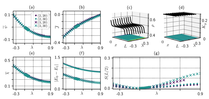
To quantify the effects of vertical boundaries on the horizontally biased dynamical phase behavior of this multi-lane ASEP, we further consider a vertically open multi-lane ASEP, where vertical entry/exit rates are $1/2$, as specified in Sec. III. In these calculations, we employed DMRG to study the ASEP behavior as a function of the horizontal bias, $\lambda_{x}$, near $\lambda_{x}=0$, with $p_{x}=0.1$ for systems of up to length $L_{x}=50$ with up to three lanes ($L_{y}=3$) using a maximum bond dimension of $D=50$.

The results are displayed in Fig. 7, with the cumulant generating function, current, current susceptibility, and first excited state gap being shown in subfigures (a), (b), (e), and (f). The per site macroscopic observables are nearly indistinguishable for the various system sizes, with the only noticeable difference caused by the requisite shifting of the point of GC symmetry as a function of system length. While in the closed multi-lane model the current detected a transition into the HD+LD phase, no such transition is apparent here.

This is further supported by a microscopic analysis for a lattice of size $2\times 20$. The density and activity profiles are shown in Fig. 7 (c) and (d) as a function of $\lambda$ and with more detailed observable information in the snapshots at $\lambda=-0.3$ and $\lambda=0.3$, shown respectively in Fig. 6 (b) and (d). The $\lambda$ sweep show no changes in the behavior of the density and vertical activity. This is also true at $\lambda=0$, where the phase transition would be expected to occur. The snapshots show no distinguishable differences in the density profiles in the regions where the MC and HD+LD phases would be expected. While the steady-state number of hops between lattice sites does not seem to indicate any phase transition, evidenced in the snapshots by comparisons of the vertical hopping rates between lanes, we note that the desired low current behavior is created in a MC-like density profile by causing a small current to flow to the left in the bulk to counter the large current flowing to the right at the boundaries. This also illustrates a significant difference between the single-lane and multi-lane systems, namely that the steady-state current need not be spatially homogenous.

The lack of the phase transition in the open multi-lane system contrasts with the behaviour of the closed multi-lane system. The behavior of the open model likely arises due to the availability of a vertical particle bath that enables rapid relaxation when jammed phases begin to form.

V Conclusions

In conclusion, we have used MPS and DMRG to conduct a systematic study of the 1D and multi-lane ASEP with open horizontal boundary conditions under a current bias. In addition to providing a simple numerical route to compute macroscopic quantities out of equilibrium, such as the cumulant generating function and its derivatives, these methods also provide access to details of the underlying microscopic configurations. We find that the entanglement entropy and spectrum provides a global summary of the correlations in the system, identifying the sharp structure of the transition into the HD+LD phase in the 1D ASEP. This transition is additionally marked by changes in the steady-state density and activity profiles. In the case of the multi-lane ASEP, we find that the shock and HD+LD phases develop when vertical particle entry/exit is prohibited, but the phase boundary disappears entirely when this is reintroduced. This emphasizes the complex interplay between vertical and horizontal hopping parameters in this class of boundary driven processes.

The MPS and DMRG are numerical realizations of the matrix ansatz method that has long been used to produce semi-analytical solutions in driven lattice models. As this and other recent work shows Bañuls and Garrahan (2019), the flexibility of the purely numerical approach allows this framework to be applied to problems where analytical techniques are difficult to use, such as the multi-lane ASEP. In addition, more general tensor network approaches beyond MPS and DMRG allow for a natural treatment of two-dimensional, three-dimensional, and thermodynamic lattice systems Verstraete et al. (2008); Orús (2014); Phien et al. (2015). Applying these to two- and three-dimensional nonequilibrium statistical models is an exciting possibility in the future.