Anomaly Inflow for M5-branes on Punctured Riemann Surfaces

Abstract

We derive the anomaly polynomials of 4d ${\cal N}=2$ theories that are obtained by wrapping M5-branes on a Riemann surface with arbitrary regular punctures, using anomaly inflow in the corresponding M-theory setup. Our results match the known anomaly polynomials for the 4d ${\cal N}=2$ class ${\cal S}$ SCFTs. In our approach, the contributions to the ’t Hooft anomalies due to boundary conditions at the punctures are determined entirely by $G_{4}$-flux in the 11d geometry. This computation provides a top-down derivation of these contributions that utilizes the geometric definition of the field theories, complementing the previous field-theoretic arguments.

1 Introduction

Geometric engineering has become a standard tool for constructing and exploring quantum field theories, especially in their strong coupling regimes. A large class of generically strongly coupled QFTs in four dimensions is realized in M-theory by wrapping a stack of M5-branes on a Riemann surface with defects. These constructions fit in the larger framework of the class $\mathcal{S}$ program, in which 4d QFTs are obtained by dimensional reduction of a 6d SCFT, generically with a partial topological twist. In this work we focus on the case of the 6d (2,0) theory of type $A_{N-1}$, which is the worldvolume theory on a stack of $N$ M5-branes. Depending on the choice of twist, the theories of class ${\cal S}$ can preserve ${\cal N}=2$ or ${\cal N}=1$ supersymmetry. The ${\cal N}=2$ theories were first constructed in Gaiotto:2009we ; Gaiotto:2009hg , building on work in Witten:1997sc . A large class of ${\cal N}=1$ theories of class ${\cal S}$ were constructed in Bah:2011vv ; Bah:2012dg , building on work in Maruyoshi:2009uk ; Benini:2009mz ; Bah:2011je . Strong evidence for the existence of these SCFTs is the construction of their large-$N$ gravity duals. The holographic duals of the ${\cal N}=2$ theories were identified in Gaiotto:2009gz , and for the ${\cal N}=1$ theories in Bah:2011vv ; Bah:2012dg ; Bah:2013qya ; Bah:2015fwa .

’t Hooft anomalies provide crucial insight into the properties of QFTs, and are especially useful observables in the study of strongly coupled theories. In an interacting SCFT, anomalies are related to central charges by the superconformal algebra Kuzenko:1999pi ; Anselmi:1997am ; in a free theory, they directly specify the matter content. Thus, they provide a measure of the degrees of freedom in a QFT. The anomalies of a $d$-dimensional QFT can be organized in a $(d+2)$-form known as the anomaly polynomial, which is a polynomial in the curvatures of background gauge and gravitational fields associated to global symmetries AlvarezGaume:1983ig ; AlvarezGaume:1984dr ; Bardeen:1984pm . The geometric nature of anomalies makes them especially amenable to computation in geometrically engineered constructions.

The 6-form ’t Hooft anomaly polynomial for a 4d theory of class $\mathcal{S}$ depends on the parent 6d theory, on the genus-$g$, $n$-punctured Riemann surface $\Sigma_{g,n}$ used in the compactification, and on the boundary conditions for the 6d theory at the punctures. The total anomaly polynomial $I_{6}^{\rm CFT}$ can be decomposed as a sum of a “universal” or “bulk” term, and of individual terms for each puncture Bah:2018gwc ,

$$I_{6}^{\text{CFT}}=I_{6}^{\text{CFT}}(\Sigma_{g,n})+\sum_{\alpha=1}^{n}I_{6}^{\text{CFT}}(P_{\alpha})\ .$$ (1.1)

The bulk term $I_{6}^{\text{CFT}}(\Sigma_{g,n})$ depends on the surface only through its Euler characteristic, $\chi(\Sigma_{g,n})=-2(g-1)-n$, and is insensitive to the choice of boundary conditions at the punctures. This contribution for the ${\cal N}=2$ theories of class ${\cal S}$ was first computed in Gaiotto:2009gz using S-duality, and can be computed by integrating the 8-form anomaly polynomial of the 6d theory over the Riemann surface Alday:2009qq ; Bah:2011vv ; Benini:2009mz ; Bah:2012dg .

The individual puncture contribution $I_{6}^{\text{CFT}}(P_{\alpha})$ depends on the choice of boundary conditions at the puncture $P_{\alpha}$, and contains information about the ’t Hooft anomalies of the flavor symmetry associated to it. These contributions can be obtained by S-duality and anomaly matching arguments Gaiotto:2009gz ; Chacaltana:2010ks ; Chacaltana:2012zy ; Tachikawa:2015bga .

The main goal of this paper is a first-principles derivation of the anomalies of the ${\cal N}=2$ class ${\cal S}$ theories of type $A_{N-1}$ from their geometric construction via M5-branes. Using anomaly inflow in M-theory, we determine both the bulk term $I_{6}^{\text{CFT}}(\Sigma_{g,n})$ and the puncture term $I_{6}^{\text{CFT}}(P_{\alpha})$, for any regular puncture. Our analysis is inspired and motivated by the holographic duals of these theories Gaiotto:2009gz . The present work is a follow up to Bah:2018jrv , where the results of the computation and main features of the derivation were presented.

The outline of the rest of the paper is as follows. In section 2 we provide an overview of the main strategy used in the computation of the inflow anomaly polynomial. In section 3 we describe in greater detail the M5-brane setup, and we discuss the bulk contribution to anomaly inflow. Section 4 is devoted to the discussion of the local geometry and $G_{4}$-flux configuration near a puncture. These data are used in section 5 to compute the puncture contribution to anomaly inflow. In section 6 we compare the total inflow result with the known CFT anomaly polynomial. In the conclusion we summarize our findings and discuss future directions. Some technical aspects of our derivation are relegated to the appendices, together with useful background material.

2 Outline of Computation

Our goal is an anomaly-inflow derivation of the ’t Hooft anomaly polynomial of 4d $\mathcal{N}=2$ class $\mathcal{S}$ theories with regular punctures. In this section we provide a summary and overview of the strategy used in the main computations in this paper.

Anomaly cancellation for M5-branes in M-theory was analyzed in Duff:1995wd ; Witten:1996hc ; Freed:1998tg ; Harvey:1998bx ; Intriligator:2000eq ; Yi:2001bz . The quantum anomaly generated by the chiral degrees of freedom localized on the M5-brane stack is cancelled by a classical inflow from the 11d ambient space. In section 2.1, we briefly review this mechanism and argue that it can be neatly summarized by introducing a 12-form characteristic class $\mathcal{I}_{12}$. The class $\mathcal{I}_{12}$ is related via standard descent relations to the classical anomalous variation of the 11d action, see (2.7), (2.8) below. Upon integrating $\mathcal{I}_{12}$ along the $S^{4}$ surrounding the M5-brane stack, one recovers the 8-form anomaly polynomial of the 6d $(2,0)$ theory of type $A_{N-1}$, up to the decoupling of center-of-mass modes.

In this work we study 4d theories obtained by considering an M5-brane stack with worldvolume $W_{6}=W_{4}\times\Sigma_{g,n}$, where $W_{4}$ is external 4d spacetime and $\Sigma_{g,n}$ is a Riemann surface of genus $g$ with $n$ punctures. In section 2.2, we consider the case without punctures, and argue that the 6-form anomaly polynomial of the resulting 4d theory can be computed by integrating $\mathcal{I}_{12}$ on a suitable 6d space $M_{6}$, which is an $S^{4}$ fibration over $\Sigma_{g,0}$. In section 2.3, we outline a two-step procedure for introducing punctures. Firstly, one constructs a modified version of $M_{6}$, by excising $n$ small disks from the Riemann surface, together with the $S^{4}$ fibers on top of them. Secondly, the “holes” in $M_{6}$ are “filled” with new geometries supported by non-trivial $G_{4}$-flux. The latter encode all data about the punctures.

2.1 Anomaly Inflow and the Class $\mathcal{I}_{12}$

Consider a stack of $N$ coincident M5-branes with a smooth 6d worldvolume $W_{6}$. The 11d tangent bundle of the ambient space $M_{11}$, restricted to $W_{6}$, decomposes as

$$TM_{11}|_{W_{6}}=TW_{6}\oplus NW_{6}\ ,$$ (2.1)

where $TW_{6}$, $NW_{6}$ are the tangent bundle and normal bundle to the M5-brane stack, respectively. The normal bundle $NW_{6}$ is isomorphic to a small tubular neighborhood of $W_{6}$ inside $M_{11}$. From this point of view, the M5-brane stack sits at the origin of the $\mathbb{R}^{5}$ fibers of $NW_{6}$, which encode the five directions transverse to the stack. The normal bundle admits an $SO(5)$ structure group. It induces an $SO(5)$ action onto the degrees of freedom on the brane; this is identified with the R-symmetry of the quantum field theory living on the branes.

The M5-brane stack acts as a singular magnetic source for the M-theory 4-form flux $G_{4}$. The Bianchi identity $dG_{4}=0$ is modified to

$$dG_{4}=2\pi\,N\,\delta^{5}(y)\,dy^{1}\wedge dy^{2}\wedge dy^{3}\wedge dy^{4}\wedge dy^{5}\ ,$$ (2.2)

where $y^{A}$, $A=1,\dots,5$, are local Cartesian coordinates in the $\mathbb{R}^{5}$ fibers of $NW_{6}$, and $\delta^{5}(y)$ is the standard 5d delta function. The relation (2.2) should only be considered as a schematic expression. As explained in Freed:1998tg ; Harvey:1998bx , (2.2) must be improved in two respects in order to implement anomaly inflow.

In the first step, we regularize the delta-function singularity in (2.2). This is achieved by excising a small tubular neighborhood $B_{\epsilon}$ of radius $\epsilon$ of the M5-brane stack. Next, we introduce a radial bump function $f(r)$, with $r$ denoting the radial coordinate $r^{2}=\delta_{AB}y^{A}y^{B}$. The function $f$ is equal to $-1$ at $r=\epsilon$, and approaches $0$ monotonically as we increase $r$. The relation (2.2) is thus replaced by

$$dG_{4}=2\pi\,N\,df\wedge{\rm vol}_{S^{4}}\ .$$ (2.3)

The 4-form ${\rm vol}_{S^{4}}$ is the volume form on the $S^{4}$ surrounding the origin of the $\mathbb{R}^{5}$ transverse directions, normalized to integrate to $1$.

The second step is to gauge the $SO(5)$ action of the normal bundle. This requires that we replace $N\,{\rm vol}_{S^{4}}$ with a multiple of the global angular form,

$$\frac{dG_{4}}{2\pi}=df\wedge E_{4}\ .$$ (2.4)

Let us stress that, in our notation, we absorb the factor $N$ inside $E_{4}$,

$$\int_{S^{4}}E_{4}=N\ .$$ (2.5)

The closed and $SO(5)$ invariant 4-form $E_{4}$ is constructed with the coordinates $y^{A}$ and the $SO(5)$ connection $\Theta_{[AB]}$ on $NW_{6}$. We refer the reader to appendix A.2 for the explicit expression of $E_{4}$.

After excising a small tubular neighborhood $B_{\epsilon}$ of the M5-brane stack, the 11d spacetime $M_{11}$ acquires a non-trivial boundary $M_{10}$ at $r=\epsilon$, which is an $S^{4}$ fibration over the worldvolume $W_{6}$,

$$M_{10}\equiv\partial(M_{11}\setminus B_{\epsilon})\ ,\qquad S^{4}\hookrightarrow M_{10}\rightarrow W_{6}\ .$$ (2.6)

The M-theory effective action $S_{\rm M}$ on $M_{11}\setminus B_{\epsilon}$ is no longer invariant under diffeomorphisms and gauge transformations of the M-theory 3-form $C_{3}$. The classical variation of the action $S_{M}$ under such a transformation takes the form

$$\frac{\delta S_{\rm M}}{2\pi}=\int_{M_{10}}\mathcal{I}_{10}^{(1)}\ ,$$ (2.7)

where $\mathcal{I}_{10}^{(1)}$ is a 10-form proportional to the gauge parameters. By virtue of the Wess-Zumino consistency conditions, the quantity $\mathcal{I}_{10}^{(1)}$ is related via descent to a formal 12-form characteristic class,

$$d\mathcal{I}_{10}^{(1)}=\delta\mathcal{I}_{11}^{(0)}\ ,\qquad d\mathcal{I}_{11}^{(0)}=\mathcal{I}_{12}\ .$$ (2.8)

We are adopting a standard descent notation, with the superscript $(0)$, $(1)$ indicating the power of the variation parameter. The class $\mathcal{I}_{12}$ originates from the topological couplings in the M-theory effective action, and is given by

$$\mathcal{I}_{12}=-\frac{1}{6}\,E_{4}\wedge E_{4}\wedge E_{4}-E_{4}\wedge X_{8}\ .$$ (2.9)

We refer the reader to appendix A.4 for a review of the derivation, based on Freed:1998tg ; Harvey:1998bx . In (2.9), $X_{8}$ is the 8-form characteristic class

$$X_{8}=\frac{1}{192}\bigg{[}p_{1}(TM_{11})^{2}-4\,p_{2}(TM_{11})\bigg{]}\ ,$$ (2.10)

where $TM_{11}$ is the tangent bundle to 11d spacetime $M_{11}$, and $p_{i}(TM_{11})$ denote its Pontryagin classes. Let us stress that a pullback to $M_{10}$ is implicit in (2.9).

The relevance of the 12-form characteristic class $\mathcal{I}_{12}$ stems from the fact that, upon integrating it along the $S^{4}$ transverse to the M5-brane stack, we obtain the inflow anomaly polynomial of the 6d theory living on the stack Freed:1998tg ; Harvey:1998bx ,

$$I_{8}^{\rm inflow}=\int_{S^{4}}\mathcal{I}_{12}\ .$$ (2.11)

Notice that (2.11) makes use implicitly of the fact that descent and integration over $S^{4}$ commute. We offer an argument for the previous statement in appendix A.5.

The anomaly polynomial $I_{8}^{\rm inflow}$ cancels against the quantum anomalies of the chiral degrees of freedom on the M5-brane stack. In the IR, the latter are organized into the interacting degrees of freedom of the 6d $(2,0)$ theory of type $A_{N-1}$, together with one free 6d $(2,0)$ tensor multiplet, related to the center of mass of the M5-brane stack. We may then write

$$I_{8}^{\rm inflow}+I_{8}^{\rm CFT}+I_{8}^{\rm decoup}=0\ ,$$ (2.12)

where $I_{8}^{\rm CFT}$ is the anomaly polynomial of the interacting $(2,0)$ theory, and $I_{8}^{\rm decoup}$ is the anomaly polynomial of a free $(2,0)$ tensor multiplet.

2.2 Four-Dimensional Anomalies from Integrals of $\mathcal{I}_{12}$

The discussion of the previous subsection is readily specialized to the case in which the M5-brane worldvolume is $W_{6}=W_{4}\times\Sigma_{g,0}$, where $W_{4}$ is external 4d spacetime, and $\Sigma_{g,0}$ is a Riemann surface of genus $g$ without punctures. In such a setup, the structure group of the normal bundle $NW_{6}$ is reduced from $SO(5)$ to $SO(2)\times SO(3)$ or $SO(2)\times SO(2)$, for compactifications preserving 4d $\mathcal{N}=2$ or $\mathcal{N}=1$ supersymmetry, respectively. A more detailed explanation of this point is found in section 3.1 below.

The space $M_{10}$ introduced in (2.6) is now an $S^{4}$ fibration over $W_{4}\times\Sigma_{g,0}$. The connection splits into an external part with legs on $W_{4}$ and an internal part with legs on $\Sigma_{g,0}$. The external part of the connection on $NW_{6}$ is a background gauge field for the continuous global symmetries of the 4d field theory. When these background gauge fields are turned off, the space $M_{10}$ decomposes as the product of $W_{4}$ and a 6d space, denoted $M_{6}^{n=0}$ to emphasize that we are considering a setup with no punctures. The space $M_{6}^{n=0}$ is an $S^{4}$ fibration over $\Sigma_{g,0}$,

$$S^{4}\hookrightarrow M_{6}^{n=0}\rightarrow\Sigma_{g,0}\ .$$ (2.13)

It is fixed by the supersymmetry conditions of M-theory, as discussed in section 3.1. We can now regard $M_{10}$ as an $M_{6}^{n=0}$ fibration over $W_{4}$,

$$M_{6}^{n=0}\hookrightarrow M_{10}\rightarrow W_{4}\ .$$ (2.14)

The topology of the above fibration encodes the information originally contained in (2.6).

We argue that the inflow anomaly polynomial $I_{6}^{\rm inflow}$ for the 4d field theory is given by

$$I_{6}^{\rm inflow}=\int_{M_{6}^{n=0}}\mathcal{I}_{12}\ ,$$ (2.15)

with $\mathcal{I}_{12}$ given in (2.9). We should bear in mind that, in analogy with the uncompactified case, the inflow anomaly polynomial $I_{6}^{\rm inflow}$ balances against the contributions of an interacting CFT as well as of decoupling modes,

$$I_{6}^{\rm inflow}+I_{6}^{\rm CFT}+I_{6}^{\rm decoup}=0\ .$$ (2.16)

The decoupling modes are precisely those arising from the compactification of a free 6d $(2,0)$ tensor multiplet on $\Sigma_{g,0}$. We stress that (2.16) generically fails in the case of emergent symmetries in the IR, in which case $I_{6}^{\rm inflow}$ might not capture all the anomalies of the CFT.

2.3 Inclusion of Punctures

Let us now outline a general strategy for extending (2.15) to the case of a compactification of an M5-brane stack on a Riemann surface $\Sigma_{g,n}$ of genus $g$ with $n$ punctures. Let $P_{\alpha}$ be the point on the Riemann surface where the $\alpha^{\rm th}$ puncture is located, for $\alpha=1,\dots,n$.

Our starting point is the space $M_{6}^{n=0}$ as in (2.13). Let $D_{\alpha}$ denote a small disk on the Riemann surface, centered around the point $P_{\alpha}$. We can present the space $M_{6}^{n=0}$ as

$$M_{6}^{n=0}=M_{6}^{\rm bulk}\cup\bigcup_{\alpha=1}^{n}(D_{\alpha}\times S^{4})\ ,$$ (2.17)

where $M_{6}^{\rm bulk}$ denotes the space obtained from $M_{6}^{n=0}$ by excising the small disk $D_{\alpha}$ around each point $P_{\alpha}$, together with the $S^{4}$ fiber on top of it. It follows that $M_{6}^{\rm bulk}$ is an $S^{4}$ fibration over $\Sigma_{g,n}$,

$$S^{4}\hookrightarrow M_{6}^{\rm bulk}\rightarrow\Sigma_{g,n}\ .$$ (2.18)

To introduce punctures, we replace each term $D_{\alpha}\times S^{4}$ in (2.17) with a new geometry $X_{6}^{\alpha}$ that encodes the puncture data. We denote the resulting space as $M_{6}$,

$$M_{6}=M_{6}^{\rm bulk}\cup\bigcup_{\alpha=1}^{n}X_{6}^{\alpha}\ .$$ (2.19)

Smoothness of $M_{6}$ constrains the gluing of $X_{6}^{\alpha}$ onto $M_{6}^{\rm bulk}$. In analogy with (2.14), the 10d space $M_{10}$ is an $M_{6}$ fibration over external spacetime $W_{4}$,

$$M_{6}\hookrightarrow M_{10}\rightarrow W_{4}\ .$$ (2.20)

Each local geometry $X_{6}^{\alpha}$ in (2.19) is supported by a non-trivial $G_{4}$-flux configuration, which is encoded in the class $E_{4}$ on $M_{10}$. The geometry $X_{6}^{\alpha}$, together with $E_{4}$ near the puncture, encodes the details of the puncture at $P_{\alpha}$. In contrast with (2.13), the space $X_{6}^{\alpha}$ is not an $S^{4}$ fibration over a 2d base space.

The class $E_{4}$ in $\mathcal{I}_{12}$ is understood as a globally-defined object on $M_{10}$. In this work we construct local expressions for $E_{4}$, both in the bulk of the Riemann surface and near each puncture, which are then constrained by regularity and flux quantization. These conditions turn out to be enough to determine the inflow anomaly polynomial.

The structure of $M_{6}$ in (2.19) implies that the total inflow anomaly polynomial can be written as a sum of a bulk contribution, associated to $M_{6}^{\rm bulk}$, and the individual contributions of punctures, associated to $X_{6}^{\alpha}$,

$$I_{6}^{\rm inflow}=\int_{M_{6}}\mathcal{I}_{12}=I_{6}^{\rm inflow}(\Sigma_{g,n})+\sum_{\alpha=1}^{n}I_{6}^{\rm inflow}(P_{\alpha})\ ,$$ (2.21)

where one has

$$I_{6}^{\rm inflow}(\Sigma_{g,n})=\int_{M_{6}^{\rm bulk}}\mathcal{I}_{12}\ ,\qquad I_{6}^{\rm inflow}(P_{\alpha})=\int_{X_{6}^{\alpha}}\mathcal{I}_{12}\ .$$ (2.22)

Several comments are in order regarding the decomposition (2.21). First of all, we stress that one should think of $M_{6}^{\rm bulk}$ as a space with boundaries. Accordingly, one has to assign suitable boundary conditions at the punctures for the connection in the fibration (2.18). Notice also that Bah:2018gwc

$$I_{6}^{\rm inflow}(\Sigma_{g,n})=\int_{M_{6}^{\rm bulk}}\mathcal{I}_{12}=\int_{\Sigma_{g,n}}I_{8}^{\rm inflow}\ ,$$ (2.23)

where the integration over $M_{6}^{\rm bulk}$ is performed by first integrating along the $S^{4}$ fibers, and then integrating on $\Sigma_{g,n}$. The class $I_{8}^{\rm inflow}$ is given by (2.11) and captures the anomalies of the 6d (2,0) SCFT that lives on a stack of flat M5-branes.

The local geometry $X_{6}^{\alpha}$ and its $G_{4}$-flux configuration are constrained by several consistency conditions. As mentioned earlier, we must be able to glue the local geometry $X_{6}^{\alpha}$ smoothly onto the bulk geometry $M_{6}^{\rm bulk}$. Moreover, the gluing must preserve all the relevant symmetries of the problem (including the correct amount of supersymmetry). Section 4 below is devoted to describing all the relevant features of the geometries $X_{6}^{\alpha}$ and associated $E_{4}$ configurations that describe regular punctures for $\mathcal{N}=2$ class $\mathcal{S}$ theories.

3 M5-brane Setup

This section is devoted to the description of the M-theory setup of a stack of $N$ M5-branes wrapping a Riemann surface $\Sigma_{g,n}$ of genus $g$ with $n$ punctures. In particular, we recall the properties of the normal bundle to the M5-branes in this scenario, and its role in implementing a partial topological twist of the parent 6d $(2,0)$ theory on $\Sigma_{g,n}$, which is essential to preserve supersymmetry in four dimensions. We then discuss the properties of the class $E_{4}$ and of the $S^{4}$ fibration $M_{6}^{n=0}$, introduced in (2.4) and (2.13). We proceed to analyze $M_{6}^{\rm bulk}$. This enables us to compute the bulk contribution to the inflow anomaly polynomial $\mathcal{I}_{6}^{\rm inflow}(\Sigma_{g,n})$ according to (2.21).

3.1 Normal Bundle to the M5-brane Stack

The 11d tangent space restricted to the M5-brane worldvolume decomposes according to (2.1). We are interested in the case in which the worldvolume $W_{6}$ wraps a Riemann surface $\Sigma_{g,n}$ of genus $g$ with $n$ punctures. The tangent space to $W_{6}$ decomposes according to

$$TW_{6}=TW_{4}\oplus T\Sigma_{g,n}\ .$$ (3.1)

The Chern root of $T\Sigma_{g,n}$ is denoted $\hat{t}$ and satisfies

$$\int_{\Sigma_{g,n}}\hat{t}=\chi(\Sigma_{g,n})=-2(g-1)-n\ .$$ (3.2)

We consider setups preserving $\mathcal{N}=2$ supersymmetry in four dimensions, in which the structure group of $NW_{6}$ reduces from $SO(5)$ to $SO(2)\times SO(3)$. Accordingly, $NW_{6}$ decomposes in a direct sum,

$$NW_{6}=N_{SO(2)}\oplus N_{SO(3)}\ ,$$ (3.3)

where $N_{SO(2)}$ is a bundle over $W_{6}$ with fiber $\mathbb{R}^{2}$ and structure group $SO(2)$, and $N_{SO(3)}$ is a bundle with fiber $\mathbb{R}^{3}$ and structure group $SO(3)$. Let $\hat{n}$ denote the Chern root of $N_{SO(2)}$. We can write

$$\hat{n}=-\hat{t}+\hat{n}^{\rm 4d}\ ,$$ (3.4)

where $\hat{n}^{\rm 4d}$ denotes the part of $\hat{n}$ depending on external spacetime. The part of $\hat{n}$ depending on $\Sigma_{g,n}$ is fixed to be $-\hat{t}$. This identification amounts to a topological twist of the parent 6d $(2,0)$ $A_{N-1}$ theory compactified on $\Sigma_{g,n}$, and is necessary to preserve 4d $\mathcal{N}=2$ supersymmetry Gaiotto:2009hg . The angular directions in the fibers of $NW_{6}$ are identified with the $S^{4}$ fiber in (2.13), (2.18) in the absence of punctures and in the presence of punctures, respectively.

The decomposition (3.3) suggests a presentation of the $S^{4}$ as an $S^{1}\times S^{2}$ fibration over an interval with coordinate $\mu\in[0,1]$. This is readily achieved by the following parametrization of $y^{A}$, $A=1,\dots,5$:

$$y^{1,2,3}=r\,\mu\,\hat{y}^{1,2,3}\ ,\qquad(\hat{y}^{1})^{2}+(\hat{y}^{2})^{2}+(\hat{y}^{3})^{2}=1\ ,\qquad y^{4}+i\,y^{5}=r\,\sqrt{1-\mu^{2}}\,e^{i\phi}\ .$$ (3.5)

We use the symbol $S^{2}_{\Omega}$ for the 2-sphere defined by the second relation. The isometries of $S^{2}_{\Omega}$ are related to the $SU(2)_{R}$ R-symmetry of the 4d theory. We refer the symbol $S^{1}_{\phi}$ for the circle parametrized by the angle $\phi$. Throughout this work, the angle $\phi$ has periodicity $2\pi$. The isometry of $S^{1}_{\phi}$ corresponds to the $U(1)_{r}$ R-symmetry in four dimensions. As apparent from (3.5), the circle $S^{1}_{\phi}$ shrinks for $\mu=1$, while the 2-sphere $S^{2}_{\Omega}$ shrinks for $\mu=0$.

The gauge-invariant differential for the angle $\phi$ reads

$$D\phi=d\phi-\mathcal{A}\ ,$$ (3.6)

where $\mathcal{A}$ is the total connection for the bundle $N_{SO(2)}$. The field strength of $\mathcal{A}$ is $\mathcal{F}=d\mathcal{A}$, and $\mathcal{F}/(2\pi)$ is identified with the Chern character $\hat{n}$. Both $\mathcal{A}$ and $\mathcal{F}$ can be split into an internal part, with legs on the Riemann surface, and a part with legs along external spacetime. We use the notation

$$\mathcal{A}=A_{\Sigma}+A_{\phi}\ ,\qquad\mathcal{F}=F_{\Sigma}+F_{\phi}\ ,$$ (3.7)

where the first term is the internal piece, and the second is the external piece. Thanks to (3.4), we have

$$\int_{\Sigma_{g,n}}\frac{\mathcal{F}}{2\pi}=\int_{\Sigma_{g,n}}\frac{F_{\Sigma}}{2\pi}=-\chi(\Sigma_{g,n})\ .$$ (3.8)

3.2 The Form $E_{4}$ away from Punctures

In this section we discuss the form $E_{4}$ in the bulk of the Riemann surface, i.e. away from punctures. As per the general discussion of subsection 2.3, the 4-form $E_{4}$ is a closed form invariant under the action of the structure group of the $S^{4}$ fibration $M_{6}^{\rm bulk}$. It is natural to exploit the decomposition (3.3) and use a factorized $E_{4}$ of the form

$$E_{4}=\mathcal{E}_{2}\wedge e_{2}^{\Omega}\ .$$ (3.9)

Let us explain our notation. The form $e_{2}^{\Omega}$ is the global, $SO(3)$ invariant angular form for the $N_{SO(3)}$ bundle. If we turn off the $N_{SO(3)}$ connection, the form $e_{2}^{\Omega}$ reduces to a multiple of the volume form on $S^{2}_{\Omega}$. We normalize $e_{2}^{\Omega}$ according to

$$\int_{S^{2}_{\Omega}}e_{2}^{\Omega}=1\ .$$ (3.10)

The explicit expression for $e_{2}^{\Omega}$ can be found in appendix A.2. The 2-form $\mathcal{E}_{2}$ is closed and gauge-invariant. We can write

$$\mathcal{E}_{2}=N\,\bigg{[}d\gamma\wedge\frac{D\phi}{2\pi}-\gamma\,\frac{\mathcal{F}}{2\pi}\bigg{]}\ .$$ (3.11)

The function $\gamma=\gamma(\mu)$ is constrained by regularity conditions. If we turn off all $N_{SO(2)}$ and $N_{SO(3)}$ connections, $E_{4}$ becomes proportional to the volume form on an $S^{4}$. Regularity of $E_{4}$ in the region where $S^{2}_{\Omega}$ shrinks demands $\gamma(0)=0$. The normalization of $E_{4}$, (2.5), then fixes $\gamma(1)=1$. To summarize,

$$\gamma(0)=0\ ,\qquad\gamma(1)=1\ .$$ (3.12)

Let us stress that, in our conventions, the integral of $E_{4}$ over any 4-cycle must be integrally quantized. A trivial example of a flux quantization condition is (2.5), which simply states that $E_{4}$ counts the total number of M5-branes in the stack. A more interesting example of flux quantization is the relation

$$\int_{\Sigma_{g,n}\times S^{2}_{\Omega}}E_{4}=N\,\chi(\Sigma_{g,n})\ ,$$ (3.13)

which follows from (3.8), (3.9), (3.11), and (3.12). In the integral above, $\Sigma_{g,n}\times S^{2}_{\Omega}$ denotes the 4-cycle obtained by combining the Riemann surface and $S^{2}_{\Omega}$, at fixed $\mu=1$, where $S^{1}_{\phi}$ shrinks. Even though flux quantization conditions for $E_{4}$ are straightforward in the bulk of the Riemann surface, they will play an essential role in section 4 in constraining the local puncture geometries and flux configurations.

3.3 The Bulk Contribution to Anomaly Inflow

In the previous section we have fixed a local expression for $E_{4}$ in the bulk of the Riemann surface. We are therefore in a position to compute the bulk contribution $I_{6}^{\rm inflow}(\Sigma_{g,n})$ to anomaly inflow, defined in (2.22). The derivation follows standard techniques, and makes use of a result of Bott and Cattaneo bott1999integral . We refer the reader to appendix A.6 for more details. The result reads

$$I_{6}^{\rm inflow}(\Sigma_{g,n}) =\frac{1}{12}\,\chi(\Sigma_{g,n})\,N^{3}\,\hat{n}^{\rm 4d}\,p_{1}(N_{SO(3)})$$

$$-\frac{1}{48}\,\chi(\Sigma_{g,n})\,N\,\hat{n}^{\rm 4d}\,\bigg{[}p_{1}(TW_{4})+p_{1}(N_{SO(3)})-(\hat{n}^{\rm 4d})^{2}\bigg{]}\ .$$ (3.14)

The notation $\hat{n}^{\rm 4d}$ was introduced in (3.4). The quantities $p_{1}(TW_{4})$, $p_{1}(N_{SO(3)})$ are the first Pontryagin classes of the tangent bundle to external spacetime, and the $N_{SO(3)}$ normal bundle, respectively.

The quantities $\hat{n}^{\rm 4d}$ and $p_{1}(N_{SO(3)})$ are given in terms of the 4d Chern classes as

$$\hat{n}^{\rm 4d}=2\,c_{1}^{r}\ ,\qquad p_{1}(N_{SO(3)})=-4\,c_{2}^{R}\ ,$$ (3.15)

where $c_{1}^{r}$ is a shorthand notation for the first Chern class of the 4d $U(1)_{r}$ R-symmetry bundle, while $c_{2}^{R}$ is a shorthand notation for the second Chern class of the 4d $SU(2)_{R}$ R-symmetry bundle. The bulk contribution to $I_{6}^{\rm inflow}$ then takes the form

$$I_{6}^{\rm inflow}(\Sigma_{g,n})=-\frac{1}{6}\,\chi(\Sigma_{g,n})\,(4N^{3}-N)\,c_{1}^{r}\,c_{2}^{R}-\frac{1}{24}\,\chi(\Sigma_{g,n})\,N\,c_{1}^{r}\,\bigg{[}p_{1}(TW_{4})-4\,(c_{1}^{r})^{2}\bigg{]}\ .$$ (3.16)

4 Introduction of Punctures

In this section we discuss punctures and analyze the properties of the local geometries $X_{6}^{\alpha}$ introduced in section 2.3. This analysis can be carried out separately for each puncture. Therefore in what follows, we omit the puncture label $\alpha$, and write $X_{6}$ for $X_{6}^{\alpha}$, $X_{4}$ for $X_{4}^{\alpha}$, and so on. We demonstrate that the puncture data are encoded in monopole sources for a suitable circle fibration, and we analyze the form of $E_{4}$ in the vicinity of a puncture.

4.1 Warm-up: Reformulation of a Non-puncture

According to the strategy outlined in section 2.3, a non-trivial puncture can be described by removing a small disk $D$ from the Riemann surface and replacing $D\times S^{4}$ with a new geometry $X_{6}$. In order to gain insight into the properties of $X_{6}$ for punctures, we first analyze the case of a non-puncture, i.e. we set $X_{6}=D\times S^{4}$ and seek a reformulation of this trivial geometry that is best suited for generalizations to non-trivial spaces. We show that $X_{6}=D\times S^{4}$ can be recast as an $S^{2}_{\Omega}$ fibration over a 4d space $X_{4}$, which is in turn a circle fibration over $\mathbb{R}^{3}$. We also provide a reformulation of the class $E_{4}$ that will prove beneficial in the discussion of genuine punctures.

Geometry for the Non-puncture

Our starting point is $X_{6}=D\times S^{4}$. The disk $D$ is parametrized by standard polar coordinates $(r_{\Sigma},\beta)$. As usual, $S^{4}$ is realized as an $S^{1}_{\phi}\times S^{2}_{\Omega}$ fibration over the $\mu$ interval. The line element on $X_{6}$ is simply

$$ds^{2}(X_{6})=dr_{\Sigma}^{2}+r_{\Sigma}^{2}\,d\beta^{2}+\frac{d\mu^{2}}{1-\mu^{2}}+(1-\mu^{2})\,D\phi^{2}+\mu^{2}\,ds^{2}(S^{2}_{\Omega})\ ,\qquad D\phi=d\phi-A_{\Sigma}\ .$$ (4.1)

We have recalled that $S^{1}_{\phi}$ is fibered over the Riemann surface with a connection $A_{\Sigma}$. For simplicity, we have temporarily turned off all external connections. The connection $A_{\Sigma}$ on the disk $D$ can be taken to be of the form

$$A_{\Sigma}=U(r_{\Sigma})\,d\beta\ ,$$ (4.2)

where the function $U$ goes to zero as $r_{\Sigma}\rightarrow 0$ to ensure that $A_{\Sigma}$ is defined at the center of the disk. The 2d space spanned by $r_{\Sigma}$ and $\mu$ is a half strip in the $(r_{\Sigma},\mu)$ plane, described by

$$r_{\Sigma}\geq 0\ ,\qquad 0\leq\mu\leq 1\ ,$$ (4.3)

see figure 1 plot (a). More precisely, the interior of the disk $D$ corresponds to a region of the form $r_{\Sigma}<r_{0}$, with $r_{0}$ constant, which is the shaded region in figure 1 plot (a).

Let us introduce a new angular coordinate $\chi$, defined by

$$\chi=\phi+\beta\ .$$ (4.4)

We can rewrite the line element (4.1) in the form

$$ds^{2}(X_{6}) =ds^{2}(X_{4})+\mu^{2}\,ds^{2}(S^{2}_{\Omega})\ ,$$

$$ds^{2}(X_{4}) =ds^{2}(B_{3})+R^{2}_{\beta}\,D\beta^{2}\ ,$$

$$ds^{2}(B_{3}) =dr_{\Sigma}^{2}+\frac{d\mu^{2}}{1-\mu^{2}}+\frac{r_{\Sigma}^{2}\,(1-\mu^{2})}{R^{2}_{\beta}}\,d\chi^{2}\ ,$$ (4.5)

where we have introduced

$$D\beta=d\beta-L\,d\chi\ ,\qquad L=\frac{1-\mu^{2}}{R^{2}_{\beta}}\ ,\qquad R^{2}_{\beta}=r^{2}_{\Sigma}+(1+U)^{2}\,(1-\mu^{2})\ .$$ (4.6)

We have reinterpreted $X_{6}$ as an $S^{2}_{\Omega}$ fibration over a 4d space $X_{4}$. The latter is in turn written as an $S^{1}_{\beta}$ fibration with connection $L\,d\chi$ over the 3d base space $B_{3}$ parametrized by $(r_{\Sigma},\mu,\chi)$. We can make the following observations:

1. The $S^{2}_{\Omega}$ shrinks on the locus $(\mu=0,r_{\Sigma}\geq 0)$, the thick black line in figure 1 plot (a).

2. In the $(r_{\Sigma},\mu)$ strip, the only point where the $D\beta$ circle shrinks is $(r_{\Sigma},\mu)=(0,1)$, where the dot-dashed blue line and the dashed red line meet in figure 1 plot (a).

3. The $\chi$ circle in the 3d base space (which is specified in $X_{4}$ by $D\beta=0$, as opposed to $d\beta=0$) shrinks on the loci $(r_{\Sigma}=0,0\leq\mu\leq 1)$ and $(\mu=1,r_{\Sigma}\geq 0)$, which correspond to the dot-dashed blue line and the dashed red line in figure 1 plot (a), respectively.

4. The function $L$ is smooth in the interior of the $(r_{\Sigma},\mu)$ strip. Moreover, $L(r_{\Sigma},\mu)=1$ on the locus $(r_{\Sigma}=0,0\leq\mu\leq 1)$, i.e. on the dot-dashed blue line. Similarly, $L(r_{\Sigma},\mu)=0$ on the locus $(\mu=1,r_{\Sigma}\geq 0)$, i.e. on the dashed red line.

We see that $L$ has a discontinuity at the point $(r_{\Sigma},\mu)=(0,1)$ where the $D\beta$ circle shrinks. The metric on $X_{4}$ near this point can be modeled by a single-center Taub-NUT space, showing that the $D\beta$ fibration has a monopole source. We write the Taub-NUT metric as

$$ds^{2}({\rm TN}) =V^{-1}\,D\beta^{2}+V\,(d\rho^{2}+d\eta^{2}+\rho^{2}\,d\chi^{2})\ ,$$

$$dD\beta =-*_{\mathbb{R}^{3}}dV\ ,\qquad V=\frac{1/2}{\sqrt{\rho^{2}+(\eta-\eta_{\rm max})^{2}}}\ ,$$ (4.7)

where $\rho$, $\eta$, $\chi$ are standard cylindrical coordinates on $\mathbb{R}^{3}$. The factor $1/2$ is related to the fact that, in our conventions, $\beta$ has periodicity $2\pi$. The coordinates $\rho$, $\eta$ are related to $r_{\Sigma}$, $\mu$ by

$$\rho=r_{\Sigma}\,\sqrt{1-\mu^{2}}\ ,\qquad\eta=\eta_{\rm max}+\frac{1}{2}(r_{\Sigma}^{2}-1+\mu^{2})\ ,$$ (4.8)

as verified by comparing $ds^{2}(X_{4})$ and $ds^{2}({\rm TN})$ near $(r_{\Sigma},\mu)=(0,1)$, with $U=0$ for simplicity.

Figure 1: The plot on the left depicts the $(r_{\Sigma},\mu)$ strip, with $r_{\Sigma}$ on the horizontal axis, and $\mu$ on the vertical axis. Lines of constant $\mu$ (solid, grey) and lines of constant $r_{\Sigma}$ (dashed, grey) are also included. The plot on the right depicts the $(\rho,\eta)$ quadrant, with $\rho$ on the horizontal axis, and $\eta$ on the vertical axis. We include the image of lines of constant $\mu$ and $r_{\Sigma}$. The shaded regions in both plots correspond to the subregion $r_{\Sigma}<r_{0}$, with $r_{0}$ constant.

The coordinate change (4.8) near $(r_{\Sigma},\mu)=(0,1)$ is a specific example of a general class of maps with the qualitative features depicted in figure 1 plot (b). First of all, the $(r_{\Sigma},\mu)$ half strip is mapped to the quadrant in the $(\rho,\eta)$ plane with $\eta\geq 0$, $\rho\geq 0$. Second of all, the thick black line is mapped to $\eta=0$. Finally, the union of the dot-dashed blue line and the dashed red line is mapped to the $\eta$ semi-axis. The corner $(r_{\Sigma},\mu)=(0,1)$ is mapped to the point $\eta=\eta_{\rm max}$ on the $\eta$ axis. The dot-dashed blue line is mapped to the region $0\leq\eta\leq\eta_{\rm max}$, while the dashed red line is mapped to $\eta\geq\eta_{\rm max}$. Figure 1 plot (b) also shows the shaded region corresponding to the interior of the disk $D$ in the new coordinates $(\rho,\eta)$.

We have shown that the space $X_{6}=D\times S^{4}$ can be reformulated as an $S^{2}_{\Omega}$ fibration over a space $X_{4}$, which is in turn a non-trivial $S^{1}_{\beta}$ fibration over $\mathbb{R}^{3}$, parametrized by cylindrical coordinates $(\rho,\eta,\chi)$,

$$S^{2}_{\Omega}\hookrightarrow X_{6}\rightarrow X_{4}\ ,\qquad S^{1}_{\beta}\hookrightarrow X_{4}\rightarrow\mathbb{R}^{3}\ .$$ (4.9)

In the above discussion, we have not included the external connection $A_{\phi}$ for $\phi$. If we turn $A_{\phi}$ on, (4.4) indicates that $d\chi$ should be replaced everywhere by

$$D\chi=d\chi-A_{\phi}\ .$$ (4.10)

In particular, we must replace $d\chi$ with $D\chi$ inside $D\beta$, thus obtaining the quantity

$$\widetilde{D\beta}=d\beta-L\,D\chi\ .$$ (4.11)

The Form $E_{4}$ for the Non-puncture

As explained in section 3.2, the form $E_{4}$ away from punctures takes the form (3.9) with $\mathcal{E}_{2}$ given by (3.11). In light of the results of the previous section, we seek a re-writing of $\mathcal{E}_{2}$ in terms of the 1-forms $D\chi$ and $\widetilde{D\beta}$ introduced in (4.10), (4.11), respectively. We are thus led to consider the ansatz

$$\mathcal{E}_{2}=d\bigg{[}Y\,\frac{D\chi}{2\pi}-W\,\frac{\widetilde{D\beta}}{2\pi}\bigg{]}\ ,$$ (4.12)

where $Y$, $W$ are functions of $\rho$, $\eta$. In order to match the above $\mathcal{E}_{2}$ with (3.11) we have to set

$$Y(\rho,\eta)=N\,\gamma\,\Big{[}1-(1+U)\,L\Big{]}\ ,\qquad W(\rho,\eta)=N\,\gamma\,(1+U)\ .$$ (4.13)

Along the $\eta$ axis, $Y$ is piecewise constant,

$$Y(0,\eta)=\left\{\begin{array}[]{ll}0&\qquad\text{for $0<\eta<\eta_{\rm max}$}\ ,\\ N&\qquad\text{for $\eta>\eta_{\rm max}$}\ .\end{array}\right.$$ (4.14)

In particular, $Y$ is discontinuous at $\eta=\eta_{\rm max}$. In contrast, $W$ is regular everywhere, because both $\gamma$ and $U$ are regular in the entire $(r_{\Sigma},\mu)$ strip, or equivalently the entire $(\rho,\eta)$ quadrant. It is worth noting that

$$W(0,\eta_{\rm max})=N\ .$$ (4.15)

Finally, we observe that both $Y$ and $W$ vanish at $\eta=0$ for any $\rho$,

$$Y(\rho,0)=0\ ,\qquad W(\rho,0)=0\ .$$ (4.16)

This is necessary to ensure regularity of $E_{4}$, and follows from the fact that $Y$ and $W$ are proportional to $\gamma$. Recall the factorized form (3.9) and that $e_{2}^{\Omega}$ contains the volume form on $S^{2}_{\Omega}$, which shrinks at $\eta=0$.

Even though $L$ and $Y$ are discontinuous along the $\eta$ axis at $\eta=\eta_{\rm max}$, the form $\mathcal{E}_{2}$ is smooth there. To check this, we write $\mathcal{E}_{2}$ in the form

$$\mathcal{E}_{2}=(dY+W\,dL+L\,dW)\,\frac{D\chi}{2\pi}-(Y+L\,W)\frac{F_{\phi}}{2\pi}-dW\,\frac{d\beta}{2\pi}\ .$$ (4.17)

The terms $dY$ and $dL$ are a potential source of $\delta$ function singularities,

$$dY\Big{|}_{\rho=0}=(+N)\,\delta(\eta-\eta_{\rm max})\,d\eta\ ,\qquad dL\Big{|}_{\rho=0}=(-1)\,\delta(\eta-\eta_{\rm max})\,d\eta\ ,$$ (4.18)

where the prefactor of the $\delta$ function is simply the jump of $Y$, $L$ across $\eta_{\rm max}$. As we can see, the $\delta$ function singularities cancel against each other in (4.17), by virtue of (4.15). Notice also that the function $Y+L\,W$ is continuous along the $\eta$ axis across the monopole location.

4.2 Local Geometry and Form $E_{4}$ for a Puncture

We are now in a position to discuss the geometry and the form $E_{4}$ for non-trivial punctures. In this section we show that all puncture data are encoded in the fluxes of $E_{4}$ along the non-trivial 4-cycles of the geometry $X_{6}$.

Geometry for a Puncture

The reformulation of the non-puncture geometry of section 4.1 provides a natural starting point for the construction of a genuine puncture geometry $X_{6}$, and determines the correct gluing prescription of $X_{6}$ to $M_{6}^{\rm bulk}$. We utilize the same fibration structure (4.9), repeated here for the reader’s convenience:

$$S^{2}_{\Omega}\hookrightarrow X_{6}\rightarrow X_{4}\ ,\qquad S^{1}_{\beta}\hookrightarrow X_{4}\rightarrow\mathbb{R}^{3}\ .$$ (4.19)

The space $\mathbb{R}^{3}$ is again parametrized by cylindrical coordinates $(\rho,\eta,\chi)$, and $S^{2}_{\Omega}$ shrinks at $\eta=0$. The $S^{1}_{\beta}$ fibration is of the form

$$D\beta=d\beta-L\,d\chi\ ,$$ (4.20)

but with a more general $L(\rho,\eta)$ than in the non-puncture case. In the base space $\mathbb{R}^{3}$, the relevant portion of the $(\rho,\eta)$ quadrant is a region analogous to the shaded region in figure 1 plot (b). The unshaded region outside is identified with the bulk of the Riemann surface.

In the non-puncture case, the $S^{1}_{\beta}$ fibration has only one unit-charge monopole source located at $\eta=\eta_{\rm max}$. We now consider several monopoles and allow for charges greater than one. More precisely, we consider a configuration with $p\geq 1$ monopoles, located at $(\rho,\eta)=(0,\eta_{a})$, $a=1,\dots,p$. The last monopole location is identified with $\eta_{\rm max}$, $\eta_{p}=\eta_{\rm max}$. For uniformity of notation, we also define $\eta_{0}:=0$. The function $L(\rho,\eta)$ is piecewise constant along the $\eta$ axis, with jumps across each monopole location $\eta_{a}$. We introduce the notation

$$L(0,\eta)=\ell_{a}\qquad\text{for}\qquad\eta_{a-1}<\eta<\eta_{a}\ .$$ (4.21)

We also demand

$$L(0,\eta)=0\qquad\text{for}\qquad\eta>\eta_{p}=\eta_{\rm max}\ .$$ (4.22)

This condition guarantees that, along the $\eta$ axis for $\eta>\eta_{\rm max}$, the $\chi$ circle in the base (i.e. setting $D\beta=0$) coincides with the $\phi$ circle. This allows us to glue the local puncture geometry to the bulk of the Riemann surface in a straightforward way.

The charge of the monopole at $\eta=\eta_{a}$ is measured by the discontinuity of the $L$ connection across $\eta=\eta_{a}$. If $S^{2}_{a}$ denotes a small 2-sphere of radius $\epsilon$ surrounding $\eta=\eta_{a}$ in the base space spanned by $(\rho,\eta,\chi)$, we have

$$-\int_{S^{2}_{a}}\frac{dD\beta}{2\pi}=\Big{[}L\Big{]}_{\eta=\eta_{a}-\epsilon}^{\eta=\eta_{a}+\epsilon}=\ell_{a+1}-\ell_{a}=:-k_{a}\ ,$$ (4.23)

where the quantity $k_{a}$ is a non-negative integer. Combining (4.23) and (4.22) we immediately derive the important relation

$$\ell_{a}=\sum_{b=a}^{p}k_{b}\ .$$ (4.24)

Since $k_{a}\geq 1$, the sequence $\{\ell_{a}\}_{a=1}^{p}$ is a decreasing sequence of positive integers. As a final remark, the non-puncture geometry is recovered by setting $p=1$, $k_{1}=1$.

Orbifold Singularities

A crucial aspect of the generalization from the non-puncture to a genuine puncture is the possibility of a monopole charge $k_{a}>1$. In analogy with the non-puncture case, in the vicinity of $\eta=\eta_{a}$ the space $X_{4}$ is modeled by a single-center Taub-NUT space ${\rm TN}_{k_{a}}$ with charge $k_{a}$. The latter has an $\mathbb{R}^{4}/\mathbb{Z}_{k_{a}}$ orbifold singularity. This singularity admits a minimal resolution in terms of a collection of $k_{a}-1$ copies of $\mathbb{C}\mathbb{P}^{1}$. Let $\widetilde{\rm TN}_{k_{a}}$ denote the resolved Taub-NUT space. In $\widetilde{\rm TN}_{k_{a}}$, each $\mathbb{C}\mathbb{P}^{1}$ has self-intersection number $-2$, and the $\mathbb{C}\mathbb{P}^{1}$’s form a linear chain with intersection number $+1$ between distinct, neighboring $\mathbb{C}\mathbb{P}^{1}$’s.

In the resolved geometry $\widetilde{\rm TN}_{k_{a}}$, we use the symbol $\widehat{\omega}_{a,I}$, $I=1,\dots,k_{a}-1$ to denote the Poincaré dual 2-forms to the $\mathbb{C}\mathbb{P}^{1}$ cycles resolving the singularity. The forms $\widehat{\omega}_{a,I}$ satisfy

$$\int_{\widetilde{\rm TN}_{k_{a}}}\widehat{\omega}_{a,I}\wedge\widehat{\omega}_{a,J}=-\,C_{IJ}^{\mathfrak{su}(k_{a})}\ ,$$ (4.25)

where there is no sum over $a$ and the symbol $C_{IJ}^{\mathfrak{su}(k_{a})}$ on the RHS denotes the entries of the Cartan matrix of $\mathfrak{su}(k_{a})$.

The Form $E_{4}$ for a Puncture

Let us now discuss the structure of the form $E_{4}$ near a puncture. We assume the factorized form (3.9) and the ansatz (4.12) for $\mathcal{E}_{2}$, repeated here for convenience,

$$E_{4}=\mathcal{E}_{2}\wedge e_{2}^{\Omega}+\dots\ ,\qquad\mathcal{E}_{2}=d\bigg{[}Y\,\frac{D\chi}{2\pi}-W\,\frac{\widetilde{D\beta}}{2\pi}\bigg{]}\ ,$$ (4.26)

where the dots represent terms associated to the flavor symmetry of the puncture, discussed in subsection 4.2. In order to ensure regularity of $E_{4}$, we must again demand that both $W(\rho,\eta)$ and $Y(\rho,\eta)$ vanish at $\eta=0$, as in (4.16).

In order to analyze the properties of $E_{4}$, we first have to study the non-trivial 4-cycles in the puncture geometry $X_{6}$. Below we construct two families of 4-cycles, denoted $\{\mathcal{C}_{a}\}_{a=1}^{p}$ and $\{\mathcal{B}_{a}\}_{a=1}^{p}$. As we shall see, regularity of $E_{4}$ at the monopole locations implies that flux configurations are labelled by a partition of $N$.

The 4-cycles $\{\mathcal{C}_{a}\}_{a=1}^{p}$.

For each $a=1,\dots,p-1$, the 4-cycle $\mathcal{C}_{a}$ is constructed as follows. In the $(\rho,\eta)$ quadrant, pick an arbitrary point $\mathsf{A}_{a}$ in the interior of the interval $(\eta_{a},\eta_{a+1})$ along the $\eta$ axis, and an arbitrary point $\mathsf{B}_{a}$ with $\eta=0$, $\rho>0$, see figure 2. At the point $\mathsf{A}_{a}$, the $\chi$ circle in the base, i.e. at $D\beta=0$, is shrinking. At point $\mathsf{B}_{a}$, $S^{2}_{\Omega}$ is shrinking. We thus obtain a 4-cycle with the topology of an $S^{4}$ by combining the arc $\mathsf{A}_{a}\mathsf{B}_{a}$, the $\chi$ circle in the base, and $S^{2}_{\Omega}$. The same construction can be repeated by selecting a point $\mathsf{A}_{p}$ along the $\eta$ axis in the region $\eta>\eta_{\rm max}$. We denote the corresponding 4-cycle as $\mathcal{C}_{p}$. Crucially, by virtue of (4.22), the $\chi$ circle in the base is nothing but $S^{1}_{\phi}$ for $\eta>\eta_{\rm max}$. It follows that

$$\mathcal{C}_{p}\cong S^{4}\ .$$ (4.27)

This observation allows us to fix a uniform orientation convention for all 4-cycles $\{\mathcal{C}_{a}\}_{a=1}^{p}$: we must choose the convention that ensures $\int_{\mathcal{C}_{p}}E_{4}=+N$, see (2.5).

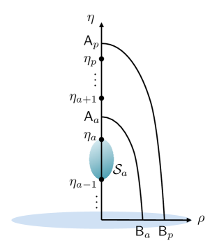
Figure 2: A generic profile of monopoles. The arcs $\mathsf{A}_{a}\mathsf{B}_{a}$ form part of the 4-cycle $\mathcal{C}_{a}$. The bubble denotes the 2-cycle $\mathcal{S}_{a}$, which is part of the 4-cycle $\mathcal{B}_{a}$.

To compute the flux of $E_{4}$ through $\mathcal{C}_{a}$, with $a=1,\dots,p-1$, we enforce $D\beta=0$ at point $\mathsf{A}_{a}$ by setting $d\beta=\ell_{a+1}\,d\chi$. We then obtain

$$\int_{\mathcal{C}_{a}}E_{4}=\int_{\mathcal{C}_{a}}e_{2}^{\Omega}\wedge d\Big{[}Y+(L-\ell_{a+1})W\Big{]}\wedge\frac{d\chi}{2\pi}=-\Big{[}Y+(L-\ell_{a+1})W\Big{]}_{\mathsf{A}_{a}}^{\mathsf{B}_{a}}=Y(\mathsf{A}_{a})\ .$$ (4.28)

In the second step, we used $\int_{S^{2}_{\Omega}}e_{2}^{\Omega}=1$, and we have recalled that $\chi$ has periodicity $2\pi$. In the final step, we utilized $W(\mathsf{B}_{a})=0$, $Y(\mathsf{B}_{a})=0$ (which follow from (4.16)) and $L(\mathsf{A}_{a})=\ell_{a+1}$ (which follows from (4.21)). While (4.28) was derived under the assumption $a=1,\dots,p-1$, it is verified that it also holds for $a=p$.

The computation (4.28) deserves further comments. First of all, since $\int_{\mathcal{C}_{a}}E_{4}$ must be quantized and the location of $\mathsf{A}_{a}$ inside the interval $(\eta_{a},\eta_{a+1})$ is arbitrary, we learn that $Y(\rho,\eta)$ is piecewise constant along the $\eta$ axis. We introduce the notation

$$Y(0,\eta) =y_{a}\in\mathbb{Z}\qquad\text{for}\qquad\eta_{a}<\eta<\eta_{a+1}\ ,\qquad a=1,\dots,p-1\ ,$$

$$Y(0,\eta) =y_{p}\in\mathbb{Z}\qquad\text{for}\qquad\eta>\eta_{p}=\eta_{\rm max}\ .$$ (4.29)

Notice that $y_{0}=0$, because $Y$ vanishes at $\eta=0$. Moreover, we can check that the orientation we chose in (4.28) is consistent. Indeed, (4.28) holds for any choice of $p$ and $k_{a}$, and in particular for the non-puncture. In that case, (4.14) shows that $Y=N$ along the $\eta$ axis for $\eta>\eta_{\rm max}$. We thus recover the expected relation $\int_{\mathcal{C}_{1}}E_{4}=+N$.

The identification (4.27) provides the boundary condition

$$y_{p}=N\ .$$ (4.30)

For any puncture, supersymmetry requires that the flux of $E_{4}$ through all the $\mathcal{C}_{a}$ carry the same sign. It follows that

$$y_{a}>0\qquad\text{for}\qquad a=1,\dots,p-1\ .$$ (4.31)

The 4-cycles $\{\mathcal{B}_{a}\}_{a=1}^{p}$.

For $a=2,3,\dots,p$, we can construct a 4-cycle $\mathcal{B}_{a}$ as follows. Consider the interval $[\eta_{a-1},\eta_{a}]$ on the $\eta$ axis. The circle $S^{1}_{\beta}$ shrinks at the location of the monopole sources, but has finite size in the interior of $[\eta_{a-1},\eta_{a}]$. As a result, we can combine $S^{1}_{\beta}$ and $[\eta_{a-1},\eta_{a}]$ and obtain a 2-cycle $\mathcal{S}_{a}$ with the topology of an $S^{2}$, depicted as a bubble in figure 2. The desired 4-cycle $\mathcal{B}_{a}$ is then simply obtained as $\mathcal{B}_{a}=\mathcal{S}_{a}\times S^{2}_{\Omega}$, since $S^{2}_{\Omega}$ has finite size in the entirety of $[\eta_{a-1},\eta_{a}]$. We can also construct a 4-cycle $\mathcal{B}_{1}$ by combining the interval $[0,\eta_{1}]$ with $S^{1}_{\beta}$ and $S^{2}_{\Omega}$. In contrast with the case $a=2,\dots,p$, the $S^{1}_{\beta}$ circle is not shrinking at the endpoint $\eta=0$. However, $S^{2}_{\Omega}$ is shrinking there, and therefore $\mathcal{B}_{1}$ is still a closed 4-cycle.

The flux of $E_{4}$ through the cycles $\{\mathcal{B}_{a}\}_{a=1}^{p}$ is computed from (4.26) by selecting the terms with one $D\beta$ factor,

$$\int_{\mathcal{B}_{a}}E_{4}=-\int_{\mathcal{B}_{a}}e_{2}^{\Omega}\wedge dW\wedge\frac{D\beta}{2\pi}=W(0,\eta_{a})-W(0,\eta_{a-1})\ .$$ (4.32)

We have recalled that $e^{\Omega}_{2}$ integrates to $1$ over $S^{2}_{\Omega}$, and that $\beta$ has periodicity $2\pi$. We have also chosen an orientation for $\mathcal{B}_{a}$.

To argue in favor of our orientation convention, we specialize (4.32) to the case of the non-puncture, $p=1$, $\eta_{1}=\eta_{\rm max}$. In that case, the cycle $\mathcal{B}_{1}$ must be equivalent to $S^{4}$, since the latter is the only non-trivial 4-cycle in the non-puncture geometry. From (4.15), (4.16), we immediately see that the RHS of (4.32) evaluates to $+N$.

It follows from (4.32) that the jumps in the values of $W$ between consecutive monopole locations must be integers, by virtue of $E_{4}$ flux quantization. Moreover, supersymmetry demands that the flux of $E_{4}$ must have the same sign for all $\{\mathcal{B}_{a}\}_{a=1}^{p}$. Consistency with the non-puncture case requires that this sign must be positive. In conclusion, we can write

$$W(0,\eta_{a})=w_{a}\ ,\qquad w_{a}-w_{a-1}\in\mathbb{Z}_{+}\ ,\qquad w_{0}=0\ ,$$ (4.33)

where the last relation follows from (4.16). Notice that $\{w_{a}\}_{a=1}^{p}$ is an increasing sequence of positive integers.

Regularity of $E_{4}$ and partition of $N$.

The quantities $L$ and $Y$ are piecewise constant along the $\eta$ axis, with jumps at the location of the monopoles. The total form $E_{4}$, however, must be regular everywhere along the $\eta$ axis. The terms $dL$ and $dY$ in (4.17) are a potential source of $\delta$ function singularities in $\mathcal{E}_{2}$, since

$$dY\Big{|}_{\rho=0}=\sum_{a=1}^{p}(y_{a}-y_{a-1})\,\delta(\eta-\eta_{a})\,d\eta\ ,\qquad dL\Big{|}_{\rho=0}=\sum_{a=1}^{p}(\ell_{a+1}-\ell_{a})\,\delta(\eta-\eta_{a})\,d\eta\ .$$ (4.34)

The normalization of each $\delta$ function at a given $\eta_{a}$ is inferred from the jump of $Y$, $L$ across $\eta_{a}$, see (4.36), (4.21) respectively. We can achieve a cancellation of each $\delta(\eta-\eta_{a})$ term in (4.17) by demanding

$$0=y_{a}-y_{a-1}+w_{a}\,(\ell_{a+1}-\ell_{a})=y_{a}-y_{a-1}-w_{a}\,k_{a}\ ,$$ (4.35)

where in the last step we made use of (4.23). We know from (4.16) that $y_{0}=0$. As a result, we can use (4.35) to express the values of $y_{a}$ in terms of $w_{a}$, $k_{a}$,

$$y_{a}=\sum_{b=1}^{a}w_{b}\,k_{b}\ .$$ (4.36)

Moreover, we have also established that $y_{p}=N$, see (4.30). Specializing (4.36) to $a=p$ we thus obtain a crucial sum rule for the flux data $w_{a}$, $k_{a}$,

$$N=\sum_{a=1}^{p}w_{a}\,k_{a}\ .$$ (4.37)

Recall that $\{w_{a}\}_{a=1}^{p}$ is an increasing sequence of positive integers, see (4.33). Moreover, all $k_{a}$ are integer and positive. It follows that the relation (4.37) defines a partition of $N$, which can be equivalently encoded in a Young diagram. Figure 3 exemplifies the translation of (4.37) into a Young diagram, in the conventions used throughout this work.

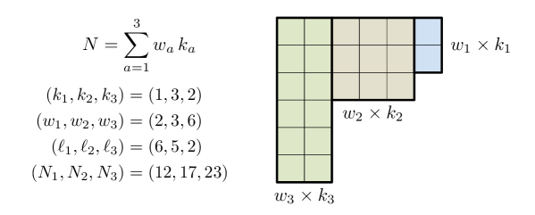
Figure 3: An example of a flux configuration for $N=23$ and associated Young diagram. The configuration has $p=3$ monopole sources with prescribed $k_{a}$, $w_{a}$. We highlighted the decomposition of the Young diagram in rectangular blocks of dimensions $w_{a}\times k_{a}$.

It is worth noting that, thanks to (4.35), the quantity $Y+W\,L$ is continuous along the $\eta$ axis. At the monopole location $\eta=\eta_{a}$ it attains the value

$$(Y+W\,L)(0,\eta_{a})=N_{a}=\sum_{b=1}^{a-1}w_{b}\,k_{b}+w_{a}\,\ell_{a}=\sum_{b=1}^{a}(w_{b}-w_{b-1})\,\ell_{b}\ .$$ (4.38)

If we choose the last monopole $a=p$, we can use $\ell_{p}=k_{p}$ (because $L$ is zero on the $\eta$ axis for $\eta>\eta_{\rm max}$) and the sum rule (4.37) to infer $N_{p}=N$.

Flavor Symmetry

In the case of the non-puncture, i.e. $p=1$, $k_{1}=1$, the space $X_{4}$ does not admit any non-trivial 2-cycles. As soon as we consider more than one monopole source and/or monopole charges greater than one, however, the geometry $X_{4}$ contains non-trivial 2-cycles. First of all, there are the 2-cycles $\{\mathcal{S}_{a}\}_{a=2}^{p}$ introduced above (4.32), which have the topology of a 2-sphere and are obtained by combining the interval $[\eta_{a-1},\eta_{a}]$ along the $\eta$ axis with the $D\beta$ fiber direction. Let us stress once more that the $D\beta$ circle does not shrink at $\eta_{0}=0$, and therefore the first interval $[0,\eta_{1}]$ combined with $S^{1}_{\beta}$ does not yield a 2-cycle. The second class of 2-cycles in $X_{4}$ is the collection of resolution $\mathbb{C}\mathbb{P}^{1}$’s at each monopole source with $k_{a}>1$, introduced at the end of section 4.2 above.

The existence of non-trivial 2-cycles in $X_{4}$ allows us to include additional terms in $E_{4}$. The total $E_{4}$ thus reads

$$E_{4}=\mathcal{E}_{2}\wedge e_{2}^{\Omega}+\sum_{a=2}^{p}\frac{F_{a}}{2\pi}\wedge\omega_{a}+\sum_{a=1}^{p}\sum_{I=1}^{k_{a}-1}\frac{\widehat{F}_{a,I}}{2\pi}\wedge\widehat{\omega}_{a,I}\ ,$$ (4.39)

where $\mathcal{E}_{2}$ is as in (4.26). The quantities $F_{a}$, $\widehat{F}_{a,I}$ are field strengths of 4d external connections. The 2-form $\omega_{a}$ is the Poincaré dual in $X_{4}$ of the 2-cycle $\mathcal{S}_{a}$, while the 2-forms $\widehat{\omega}_{a,I}$ are the Poincaré duals of the resolution $\mathbb{C}\mathbb{P}^{1}$’s at each monopole with $k_{a}\geq 2$. (The sum over $I$ is understood to be zero if $k_{a}=1$.) The 4d connections $F_{a}$, $\widehat{F}_{a,I}$ in (4.39) are interpreted as background gauge fields for the flavor symmetry associated to the puncture. More precisely, (4.39) captures the Cartan subalgebra of the full flavor symmetry group

$$G_{F}=S\bigg{[}\prod_{a=1}^{p}U(k_{a})\bigg{]}\ .$$ (4.40)

The connections $\widehat{F}_{a,I}$ are in one-to-one correspondence with the Cartan generators of the $SU(k_{a})$ factor in $G_{F}$, while the $F_{a}$ correspond to the remaining $U(1)$ factors.

The states associated to the non-Cartan generators of $G_{F}$ are not visible in the supergravity approximation, since they originate from M2-branes wrapping the resolution $\mathbb{C}\mathbb{P}^{1}$’s. For the purpose of computing ’t Hooft anomaly coefficients, however, the form $E_{4}$ contains all necessary information.

5 Puncture Contributions to Anomaly Inflow

As explained in section 2.3, the contribution of the $\alpha^{\rm th}$ puncture to the total inflow anomaly polynomial $I_{6}^{\rm inflow}(P_{\alpha})$ is given by (2.22), with $\mathcal{I}_{12}$ given by (2.9). In this section we compute the integral in (2.22), considering the two terms in $\mathcal{I}_{12}$ in turn. For notational convenience, we suppress the puncture label $\alpha$ throughout the rest of this section.

5.1 Computation of the $(E_{4})^{3}$ Term

The total expression for the form $E_{4}$ near a puncture is given in (4.39), with $\mathcal{E}_{2}$ as in (4.26). Our task is to identify the terms in $(E_{4})^{3}$ that saturate the integral over the 6d space $X_{6}$, which is an $S^{2}_{\Omega}$ fibration over $X_{4}$, see (4.9). The Bott-Cattaneo formula, reviewed in appendix A.3, implies

$$\int_{S^{2}_{\Omega}}(e_{2}^{\Omega})^{3}=\frac{1}{4}p_{1}(N_{SO(3)})\ ,\qquad\int_{S^{2}_{\Omega}}e_{2}^{\Omega}=1\ ,$$ (5.1)

while even powers of $e_{2}^{\Omega}$ integrate to zero. It follows that

$$\int_{X_{6}}(E_{4})^{3}=\frac{1}{4}p_{1}(N_{SO(3)})\,\int_{X_{4}}(\mathcal{E}_{2})^{3}+3\,\int_{X_{4}}\mathcal{E}_{2}\wedge\bigg{[}\sum_{a=2}^{p}\frac{F_{a}}{2\pi}\wedge\omega_{a}+\sum_{a=1}^{p}\sum_{I=1}^{k_{a}-1}\frac{\widehat{F}_{a,I}}{2\pi}\wedge\widehat{\omega}_{a,I}\bigg{]}^{2}\ .$$ (5.2)

To proceed, we isolate the terms in $(\mathcal{E}_{2})^{3}$ that saturate the integration over $X_{4}$,

$$\int_{X_{4}}(\mathcal{E}_{2})^{3}=-3\int_{X_{4}}d\Big{[}(Y+W\,L)^{2}\Big{]}\wedge dW\wedge\frac{D\chi}{2\pi}\wedge\frac{\widetilde{D\beta}}{2\pi}\wedge\frac{F_{\phi}}{2\pi}\ .$$ (5.3)

The integration over the angles $\chi$, $\beta$ is readily performed. (Recall that they both have periodicity $2\pi$.) The integral of the 2-form $d[(Y+W\,L)^{2}]\wedge dW$ on the $(\rho,\eta)$ plane is discussed in detail in appendix B. Combining all elements, we arrive at

$$\int_{X_{4}}(\mathcal{E}_{2})^{3}=-\frac{F_{\phi}}{2\pi}\,\sum_{a=1}^{p}\bigg{[}2\,\ell_{a}^{2}\,(w_{a}^{3}-w_{a-1}^{3})+3\,\ell_{a}\,(N_{a}-w_{a}\,\ell_{a})\,(w_{a}^{2}-w_{a-1}^{2})\bigg{]}\ .$$ (5.4)

Let us now turn to the second $X_{4}$ integral in (5.2). In this case, integration over $X_{4}$ is saturated by considering terms quadratic in the 2-forms $\omega_{a}$, $\widehat{\omega}_{a,I}$,

$$\int_{X_{6}}(E_{4})^{3} =-3\,\frac{F_{\phi}}{2\pi}\wedge\bigg{[}\sum_{a,b=1}^{p}\sum_{I=1}^{k_{a}-1}\sum_{J=1}^{k_{b}-1}\mathcal{K}_{(a,I),(b,J)}\,\frac{\widehat{F}_{a,I}}{2\pi}\wedge\frac{\widehat{F}_{b,J}}{2\pi}$$

$$+\sum_{a,b=2}^{p}\mathcal{K}_{a,b}\,\frac{F_{a}}{2\pi}\wedge\frac{F_{b}}{2\pi}+2\,\sum_{a=2}^{p}\sum_{b=1}^{p}\sum_{J=1}^{k_{b}-1}\mathcal{K}_{a,(b,J)}\,\frac{F_{a}}{2\pi}\wedge\frac{\widehat{F}_{b,J}}{2\pi}\bigg{]}+\dots\ ,$$ (5.5)

where the coefficients are

$$\mathcal{K}_{(a,I),(b,J)} =\int_{X_{4}}(Y+W\,L)\,\widehat{\omega}_{a,I}\wedge\widehat{\omega}_{b,J}\ ,$$

$$\mathcal{K}_{a,b} =\int_{X_{4}}(Y+W\,L)\,\omega_{a}\wedge\omega_{b}\ ,$$

$$\mathcal{K}_{a,(b,J)} =\int_{X_{4}}(Y+W\,L)\,\omega_{a}\wedge\widehat{\omega}_{b,J}\ .$$ (5.6)

We have used the fact that the only relevant part of $\mathcal{E}_{2}$ is the one with legs along external spacetime, $-(Y+W\,L)F_{\phi}/(2\pi)$.

The coefficients $\mathcal{K}_{(a,I),(b,J)}$ are computed as follows. The 2-forms $\widehat{\omega}_{a,I}$ are associated to the resolution $\mathbb{C}\mathbb{P}^{1}$’s of the orbifold singularity at the $a^{\rm th}$ monopole. It follows that $\mathcal{K}_{(a,I),(b,J)}$ is only non-zero for $a=b$. As a result, the quantity $Y+WL$ is evaluated at $(\rho,\eta)=(0,\eta_{a})$, and gives a factor $N_{a}$ by virtue of (4.38). The integration over $X_{4}$ reduces to an integration over the resolved orbifold $\widetilde{\rm TN}_{k_{a}}$ and is performed using (4.25). We thus have

$$\mathcal{K}_{(a,I),(b,J)}=-\delta_{a,b}\,N_{a}\,C_{IJ}^{\mathfrak{su}(k_{a})}\ .$$ (5.7)

A computation of the coefficients $\mathcal{K}_{a,b}$ and $\mathcal{K}_{a,(b,J)}$ in (5.1) requires full control over the intersection pairing among the 2-cycles $\mathcal{S}_{a}$ and the resolution $\mathbb{C}\mathbb{P}^{1}$’s, as well as over the normalization of the 2-forms $\omega_{a}$. We refrain from a discussion of these coefficients.

Let us summarize the final result of the computation of this subsection, using (3.15) to express $\hat{n}^{\rm 4d}=F_{\phi}/(2\pi)$ and $p_{1}(N_{SO(3)})$ in terms of 4d Chern classes,

$$\int_{X_{6}}(E_{4})^{3} =2\,c_{1}^{r}\,c_{2}^{R}\,\sum_{a=1}^{p}\bigg{[}2\,\ell_{a}^{2}\,(w_{a}^{3}-w_{a-1}^{3})+3\,\ell_{a}\,(N_{a}-w_{a}\,\ell_{a})\,(w_{a}^{2}-w_{a-1}^{2})\bigg{]}$$

$$+6\,c_{1}^{r}\,\sum_{a=1}^{p}N_{a}\sum_{I,J=1}^{k_{a}-1}C_{IJ}^{\mathfrak{su}(k_{a})}\,\frac{\widehat{F}_{a,I}}{2\pi}\wedge\frac{\widehat{F}_{a,J}}{2\pi}-6\,c_{1}^{r}\,\sum_{a,b=2}^{p}\mathcal{K}_{a,b}\,\frac{F_{a}}{2\pi}\wedge\frac{F_{b}}{2\pi}$$

$$-12\,c_{1}^{r}\,\sum_{a=2}^{p}\sum_{b=1}^{p}\sum_{J=1}^{k_{b}-1}\mathcal{K}_{a,(b,J)}\,\frac{F_{a}}{2\pi}\wedge\frac{\widehat{F}_{b,J}}{2\pi}\ .$$ (5.8)

5.2 Computation of the $E_{4}\wedge X_{8}$ Term

Recall from section 4.2 that the puncture geometry $X_{4}$ has an $\mathbb{R}^{4}/\mathbb{Z}_{k_{a}}$ orbifold singularity at the location of each monopole of charge $k_{a}\geq 2$. The singularity is modeled by a single-center Taub-NUT space ${\rm TN}_{k_{a}}$, which can be resolved to $\widetilde{\rm TN}_{k_{a}}$. We use the notation $\widetilde{X}_{4}$ for the space obtained from $X_{4}$ by resolving all its orbifold singularities.

With this notation, the relevant decomposition of the 11d tangent bundle, restricted to the brane worldvolume, is

$$TM_{11}|_{W_{6}}=TW_{4}\oplus N_{SO(3)}\oplus T\widetilde{X}_{4}\ .$$ (5.9)

The above expression is motivated by the fact that the resolved space $\widetilde{X}_{4}$ is a local model of the cotangent bundle to the Riemann surface in the vicinity of the puncture.

Let $\lambda_{1}$, $\lambda_{2}$ denote the Chern roots of $T\widetilde{X}_{4}$. Since $c_{1}(T\widetilde{X}_{4})=0$, we can write

$$\lambda_{1}=-\lambda_{2}=:\lambda\ .$$ (5.10)

In our geometry, the $U(1)$ associated to the $\chi$ circle is gauged with the 4d connection $A_{\phi}$. In order to account for this fact, we shift the Chern roots of $T\widetilde{X}_{4}$,

$$\lambda_{1}^{\rm tot}:=\lambda+\tfrac{1}{2}\,\hat{n}^{\rm 4d}\ ,\qquad\lambda_{2}^{\rm tot}:=-\lambda+\tfrac{1}{2}\,\hat{n}^{\rm 4d}\ ,$$ (5.11)

where $\hat{n}^{\rm 4d}$ is the spacetime component of the Chern root of $N_{SO(2)}$ introduced in (3.4). We see from (5.11) that it is the sum of Chern roots $\lambda_{1}+\lambda_{2}$ that is shifted with $+\hat{n}^{\rm 4d}$. This is due to the definition of the angle $\chi$ in terms of $\beta$, $\phi$—see (4.4). We can now compute the shifted Pontryagin classes for $T\widetilde{X}_{4}$, including the contribution from the gauging with $\hat{n}^{\rm 4d}$,

$$p_{1}(T\widetilde{X}_{4})^{\rm tot} =(\lambda_{1}^{\rm tot})^{2}+(\lambda_{2}^{\rm tot})^{2}=p_{1}(T\widetilde{X}_{4})+\tfrac{1}{2}\,(\hat{n}^{\rm 4d})^{2}\ ,$$

$$p_{2}(T\widetilde{X}_{4})^{\rm tot} =(\lambda_{1}^{\rm tot})^{2}\,(\lambda_{2}^{\rm tot})^{2}=-\tfrac{1}{4}\,p_{1}(T\widetilde{X}_{4})\,(\hat{n}^{\rm 4d})^{2}\ ,$$ (5.12)

where $p_{1}(T\widetilde{X}_{4})$ is the first Pontryagin class of $T\widetilde{X}_{4}$ before the 4d gauging is turned on. Using (5.9), (2.10), and standard formulae for Pontryagin classes (A.18), we compute

$$X_{8} =-\frac{1}{96}\,\Big{[}p_{1}(TW_{4})+p_{1}(N_{SO(3)})-(\hat{n}^{\rm 4d})^{2}\Big{]}{p_{1}(T\widetilde{X}_{4})}+\dots\ .$$ (5.13)

We have selected the terms with one $p_{1}(T\widetilde{X}_{4})$, with the dots representing the remaining terms, which will not be important for the following discussion.

We are now in a position to integrate $E_{4}\wedge X_{8}$ over $X_{6}$. The integral in the directions of $\widetilde{X}_{4}$ is saturated by $p_{1}(T\widetilde{X}_{4})$, while the integral on $S^{2}_{\Omega}$ is saturated by $e_{2}^{\Omega}$ in the term $\mathcal{E}_{2}\wedge e_{2}^{\Omega}$ in $E_{4}$. It follows that

$$\int_{X_{6}}E_{4}\wedge X_{8}=\frac{1}{48}\,\,c_{1}^{r}\,\Big{[}p_{1}(TW_{4})+p_{1}(N_{SO(3)})-(\hat{n}^{\rm 4d})^{2}\Big{]}\,\int_{\widetilde{X}_{4}}(Y+W\,L)\,{p_{1}(T\widetilde{X}_{4})}\ .$$ (5.14)

We have already performed the integral over $S^{2}_{\Omega}$, and we have selected the only piece of $\mathcal{E}_{2}$ which is relevant, i.e. the part with $F_{\phi}=2\pi\hat{n}^{\rm 4d}$. The integral over $\widetilde{X}_{4}$ localizes onto the positions $\eta=\eta_{a}$ of the monopoles,

$$\int_{\widetilde{X}_{4}}(Y+W\,L)\,{p_{1}(T\widetilde{X}_{4})}=\sum_{a=1}^{p}N_{a}\,\int_{\widetilde{\rm{TN}}_{k_{a}}}p_{1}(T\widetilde{\rm{TN}}_{k_{a}})\ .$$ (5.15)

We exploited the fact that the quantity $Y+W\,L$ takes the value $N_{a}$ at $(\rho,\eta)=(0,\eta_{a})$, see (4.38). The integrals of the individual classes $p_{1}(T\widetilde{\rm{TN}}_{k_{a}})$ are evaluated making use of the results of Gibbons:1979gd for ALF resolutions of $\mathbb{R}^{4}/\mathbb{Z}_{k_{a}}$,

$$\int_{\widetilde{\rm{TN}}_{k_{a}}}p_{1}(T\widetilde{\rm{TN}}_{k_{a}})=2\,k_{a}\ .$$ (5.16)

In conclusion, we obtain

$$\int_{X_{6}}E_{4}\wedge X_{8}=\frac{1}{24}\sum_{a=1}^{p}N_{a}\,k_{a}\,c_{1}^{r}\,\Big{[}p_{1}(TW_{4})-4\,c_{2}^{R}-4\,(c_{1}^{r})^{2}\Big{]}\ ,$$ (5.17)

where we have expressed the result in terms of $c_{1}^{r}$, $c_{2}^{R}$ using (3.15).

6 Comparison with CFT Expectations

In this section we first summarize the total result for the inflow anomaly polynomial, and we then prove that it matches with the CFT expectation.

6.1 Summary of Inflow Anomaly Polynomial

We can assemble the contribution $I_{6}^{\rm inflow}(P_{\alpha})$ of the $\alpha^{\rm th}$ puncture to the inflow anomaly polynomial, making use of (2.22) and the findings of the previous sections. The result reads

$$I_{6}^{\rm inflow}(P_{\alpha}) =(n_{v}-n_{h})^{\rm inflow}(P_{\alpha})\,\bigg{[}\frac{1}{3}\,(c_{1}^{r})^{3}-\frac{1}{12}\,c_{1}^{r}\,p_{1}(TW_{4})\bigg{]}-n_{v}^{\rm inflow}(P_{\alpha})\,c_{1}^{r}\,c_{2}^{R}$$

$$+I_{6}^{\rm inflow,flavor}(P_{\alpha})\ ,$$ (6.1)

where the anomaly coefficients are given in terms of the quantized flux data as

$$(n_{v}-n_{h})^{\rm inflow}(P_{\alpha}) =\frac{1}{2}\,\sum_{a=1}^{p}N_{a}\,k_{a}\ ,$$

$$n_{v}^{\rm inflow}(P_{\alpha}) =\sum_{a=1}^{p}\bigg{[}\frac{2}{3}\,\ell_{a}^{2}\,(w_{a}^{3}-w_{a-1}^{3})+\ell_{a}\,(N_{a}-w_{a}\,\ell_{a})\,(w_{a}^{2}-w_{a-1}^{2})-\frac{1}{6}\,N_{a}\,k_{a}\bigg{]}\ ,$$

$$I_{6}^{\rm inflow,flavor}(P_{\alpha}) =c_{1}^{r}\bigg{[}-\sum_{a=1}^{p}N_{a}\sum_{I,J=1}^{k_{a}-1}C_{IJ}^{\mathfrak{su}(k_{a})}\,\frac{\widehat{F}_{a,I}}{2\pi}\wedge\frac{\widehat{F}_{a,J}}{2\pi}+\,\sum_{a,b=2}^{p}\mathcal{K}_{a,b}\,\frac{F_{a}}{2\pi}\wedge\frac{F_{b}}{2\pi}$$

$$\qquad\;\;\,+2\,\sum_{a=2}^{p}\sum_{b=1}^{p}\sum_{J=1}^{k_{b}-1}\mathcal{K}_{a,(b,J)}\,\frac{F_{a}}{2\pi}\wedge\frac{\widehat{F}_{b,J}}{2\pi}\bigg{]}\ .$$ (6.2)

The coefficients $\mathcal{K}_{a,b}$, $\mathcal{K}_{a,(b,J)}$ in $I_{6}^{\rm inflow,flavor}(P_{\alpha})$ are defined in (5.1). A minor comment about our notation is in order. We have reinstated the puncture label $\alpha$ on the LHS’s of the above equations. Strictly speaking, each puncture comes with its local data, and on the RHS’s we should write $p^{\alpha}$, $k_{a}^{\alpha}$, $\ell_{a}^{\alpha}$, and so on. We prefer to omit the label $\alpha$ from the RHS’s of the above relations in order to avoid cluttering the expressions.

In the piece related to flavor symmetry, we expect an enhancement of the first term to the second Chern class of the full non-Abelian $SU(k_{a})$ factor in the flavor symmetry group,

$$-c_{1}^{r}\,\sum_{a=1}^{p}N_{a}\sum_{I,J=1}^{k_{a}-1}C_{IJ}^{\mathfrak{su}(k_{a})}\,\frac{\widehat{F}_{a,I}}{2\pi}\wedge\frac{\widehat{F}_{a,J}}{2\pi}\rightarrow-2\,\sum_{a=1}^{p}2\,N_{a}\,c_{1}^{r}\,c_{2}(SU(k_{a}))\ .$$ (6.3)

The corresponding flavor central charge is

$$k_{{SU}(k_{a})}^{\rm inflow}=-2\,N_{a}\ .$$ (6.4)

For the sake of completeness, we also restate the bulk contribution of the Riemann surface to the anomalies:

$$(n_{v}-n_{h})^{\rm inflow}(\Sigma_{g,n}) =\frac{1}{2}\chi(\Sigma_{g,n})N\ ,$$ (6.5)

$$n_{v}^{\rm inflow}(\Sigma_{g,n}) =\frac{1}{6}\chi(\Sigma_{g,n})(4N^{3}-N)\ .$$ (6.6)

We would now like to compare these expressions with the anomalies of the 4d SCFT. Our results are summarized in (6.46)-(6.50).

6.2 Anomalies of the ${\cal N}=2$ Class ${\cal S}$ SCFTs

The anomaly polynomial of any 4d $\mathcal{N}=2$ SCFT with flavor symmetry $G_{F}$ can be written in the form

$$I_{6}^{\rm CFT}=(n_{v}-n_{h})\,\bigg{[}\frac{1}{3}\,(c_{1}^{r})^{3}-\frac{1}{12}\,c_{1}^{r}\,p_{1}(TW_{4})\bigg{]}-n_{v}\,c_{1}^{r}\,c_{2}^{R}-k_{G}\,c_{1}^{r}\,{\rm ch}_{2}(G_{F})\ .$$ (6.7)

This structure follows from the ${\cal N}=2$ superconformal algebra Kuzenko:1999pi . Here, ${\rm ch}_{2}(G_{F})$ is the 2-form part of the Chern character for $G_{F}$; for instance, ${\rm ch}_{2}(SU(m))=-c_{2}(SU(m))$ (see appendix A.1). The flavor central charge is defined in terms of the $G_{F}$ generators $T^{a}$ as

$$k_{G_{F}}\delta^{ab}=-2\mathop{\mathrm{tr}}\nolimits R_{{\cal N}=2}T^{a}T^{b}.$$ (6.8)

The parameters $n_{v}$ and $n_{h}$ correspond to the number of vector multiplets and hypermultiplets respectively when the theory is free, and otherwise can be regarded as an effective number of vector multiplets and hypermultiplets. These are related to the SCFT central charges as $a=\frac{1}{24}(5n_{v}+n_{h})$, and $c=\frac{1}{12}(2n_{v}+n_{h})$.

An ${\cal N}=2$ theory of class ${\cal S}$ has two contributions to their anomalies, which we denote in terms of the $n_{v}$ and $n_{h}$ parameters as

$$n_{v}^{\text{CFT}}=n_{v}^{\text{CFT}}(\Sigma_{g,n})+\sum_{\alpha=1}^{n}n_{v}^{\text{CFT}}(P_{\alpha})\ ,\qquad n_{h}^{\text{CFT}}=n_{h}^{\text{CFT}}(\Sigma_{g,n})+\sum_{\alpha=1}^{n}n_{h}^{\text{CFT}}(P_{\alpha})\ .$$ (6.9)

The bulk terms are proportional to the Euler characteristic $\chi$ of the Riemann surface,

$$(n_{v}-n_{h})^{\text{CFT}}(\Sigma_{g,n}) =-\frac{1}{2}\,\chi(\Sigma_{g,n})\,(N-1),\$$ (6.10)

$$n_{v}^{\text{CFT}}(\Sigma_{g,n}) =-\frac{1}{2}\,\chi(\Sigma_{g,n})\,\left(\frac{4}{3}N^{3}-\frac{1}{3}N-1\right)\ .$$ (6.11)

These were computed in Benini:2009mz ; Alday:2009qq by integrating the 6d (2,0) anomaly polynomial over the Riemann surface without punctures. The remaining terms in (6.9) depend on the local puncture data, which we will now review.

A regular ${\cal N}=2$ puncture is labeled by an embedding $\rho:\mathfrak{su}(2)\to\mathfrak{g}$. For $\mathfrak{g}=A_{N-1}$, $\rho$ is one-to-one with a partition of $N$, encoded in a Young diagram with $N$ boxes. Consider a Young diagram with $\widetilde{p}$ rows of length $\widetilde{\ell}_{i}$, with $i=1,\dots,\widetilde{p}$. The partition is given as

$$N=\sum_{i=1}^{\widetilde{p}}\widetilde{\ell}_{i}\ .$$ (6.12)

A puncture corresponding to this partition contributes a flavor symmetry $G_{F}$ to the 4d CFT, where $G_{F}$ is the commutant of the embedding $\rho$,

$$G_{F}=S\left[\prod_{i=1}^{\widetilde{p}}U(\widetilde{k}_{i})\right].$$ (6.13)

The quantities $\widetilde{k}_{i}$ are defined as

$$\widetilde{k}_{i} =\widetilde{\ell}_{i}-\widetilde{\ell}_{i+1}\ ,\qquad\widetilde{\ell}_{\widetilde{p}+1}\equiv 0\ ,\qquad\widetilde{\ell}_{i}=\sum_{j=i}^{\widetilde{p}}\widetilde{k}_{j}\ .$$ (6.14)

In order to write down $n_{v,h}^{\text{CFT}}(P_{\alpha})$ it is also useful to introduce the notation

$$\widetilde{\ell}_{i}=\widetilde{N}_{i}-\widetilde{N}_{i-1}\ ,\qquad\widetilde{N}_{\widetilde{p}}=\widetilde{N}_{\widetilde{p}+1}=N\ ,\qquad\widetilde{N}_{i} =\sum_{j=1}^{i}\widetilde{\ell}_{j}=\sum_{j=1}^{i-1}j\,\widetilde{k}_{j}+i\,\sum_{j=i}^{\widetilde{p}}\widetilde{k}_{j}\ .$$ (6.15)

Notice the relation $2\,\widetilde{N}_{i}-\widetilde{N}_{i+1}-\widetilde{N}_{i-1}=\widetilde{k}_{i}$, which encodes the $N_{f}=2N_{c}$ condition for the vanishing of the $\beta$ function in the dual quiver description Witten:1997sc .

The puncture contribution to the ’t Hooft anomalies of the class ${\cal S}$ SCFTs can be stated in terms of this data as follows:

$$(n_{v}-n_{h})^{\text{CFT}}(P_{\alpha}) =-\frac{1}{2}\sum_{i=1}^{\widetilde{p}}\widetilde{N}_{i}\widetilde{k}_{i}+\frac{1}{2}\ ,$$ (6.16)

$$n_{v}^{\text{CFT}}(P_{\alpha}) =-\sum_{i=1}^{\widetilde{p}}\left(N^{2}-\widetilde{N}_{i}^{2}\right)-\frac{1}{2}N^{2}+\frac{1}{2}\ ,$$ (6.17)

$${k}^{\text{CFT}}_{{SU}(\widetilde{k}_{i})} =2\widetilde{N}_{i}\ .\phantom{\frac{1}{2}}$$ (6.18)

The last equation is the mixed flavor-R-symmetry contribution due to a factor $SU(\widetilde{k}_{i})$ of the flavor group. These contributions were computed explicitly for the $A_{n}$ case in Gaiotto:2009gz ; Chacaltana:2010ks , with the general ADE formula derived in Chacaltana:2012zy .

It will also be useful to note the following expressions for $n_{v}$, $n_{h}$ associated to a free tensor multiplet reduced on a Riemann surface without punctures:

$$n_{v}^{\text{free tensor}}=-\frac{1}{2}\chi(\Sigma_{g,0})\ ,\qquad(n_{v}-n_{h})^{\text{free tensor}}=-\frac{1}{2}\chi(\Sigma_{g,0})\ .$$ (6.20)

These expressions can be found by dimensional reduction of the 8-form anomaly polynomial of a single M5-brane—see appendix C for more details.

6.3 Relating Inflow Data to Young Diagram Data

The map between the data of the Young diagram and the inflow data is as follows. Consider a profile with $p$ monopoles. The monopole located at ${\eta}_{a}$ on the $\eta$ axis has charge

$${k}_{a}={\ell}_{a}-{\ell}_{a+1}\ ,$$ (6.21)

where we used (4.23) to express $k_{a}$ in terms of $\ell_{a}$. Let us recast the sum rule (4.37) in the form

$$N=\sum_{a=1}^{p}(w_{a}-w_{a-1})\,\ell_{a}\ .$$ (6.22)

We can interpret (6.22) as a partition of $N$ determined by the Young diagram

$$\mathsf{Y}=[(\ell_{1})^{w_{1}},(\ell_{2})^{w_{2}-w_{1}},\dots,(\ell_{a})^{w_{a}-w_{a-1}},\dots,(\ell_{p})^{w_{p}-w_{p-1}}]\ .$$ (6.23)

We are using a notation in which $\mathsf{Y}$ is specified by giving the lengths of its rows. More precisely, we list the distinct lengths $\ell_{a}$ in decreasing order. The exponent of $\ell_{a}$ is the number of rows with length $\ell_{a}$.

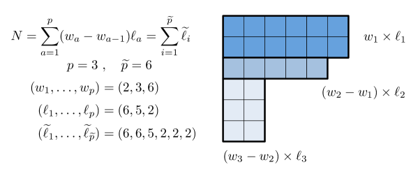
Figure 4: The example of figure 3 is reformulated in terms of $\ell_{a}$, $\widetilde{\ell}_{i}$. We highlighted the decomposition of the Young diagram in rectangular blocks of dimensions $(w_{a}-w_{a-1})\times\ell_{a}$.

The map to the rows $\widetilde{\ell}_{i}$ of the Young diagram that describes the CFT is

$$\widetilde{\ell}_{i}=\text{value of $L$ along the $\eta$ axis for $\eta\in(i-1,i)$}\ ,\qquad i=1,2,\dots,w_{p}\ .$$ (6.24)

Equivalently, we can write

$$\widetilde{\ell}_{i}=\ell_{a}\qquad\text{for all $i=w_{a-1}+1,\dots,w_{a}$ }\ .$$ (6.25)

Then, the sequence

$$(\widetilde{\ell}_{1}\ ,\widetilde{\ell}_{2}\ ,\dots\ ,\widetilde{\ell}_{\widetilde{p}}),\qquad\widetilde{p}=w_{p}\ .$$ (6.26)

is exactly the sequence of lengths of all rows of $\mathsf{Y}$, this time listed with repetitions. The total number of rows is equal to the quantity $w_{p}$. Figure 4 shows the example considered in figure 3, reformulating the partition of $N$ in terms of $\ell_{a}$ and $\widetilde{\ell}_{i}$.

We can identify the monopole charge $k_{a}$ with the $\widetilde{k}_{i}$ as

$$\widetilde{k}_{i}=\left\{\begin{array}[]{ll}0&\qquad\text{if $i\notin\{w_{a}\}_{a=1}^{p}$\ ,}\\[2.84526pt] k_{a}&\qquad\text{if $i=w_{a}$\ .}\end{array}\right.$$ (6.27)

When this is nonzero, it corresponds to a location of a monopole, and equals a corresponding $k_{a}$. Therefore we can equivalently rewrite the flavor symmetry (6.13) as

$$G_{F}=S\left[\prod_{a=1}^{p}U(k_{a})\right].$$ (6.28)

In this way, the variables that run over number-of-monopoles and those that run over number-of-rows are related by taking into account the multiplicity of rows of the same length.

Before going on, we pause to go through several examples of puncture profiles, mapping the Young diagram data to the inflow data and computing the anomaly contributions of the punctures. We draw the corresponding Young diagrams for the case of $N=4$ in figure 5.

Example 1: Non-puncture

The Young diagram data that labels a non-puncture (no flavor symmetry) is:

$$\begin{split}\text{non-puncture}:\qquad&\widetilde{p}=N,\quad\widetilde{\ell}_{i=1,\dots,N}=1,\quad(\widetilde{k}_{i=1,\dots,N-1}=0,\ \widetilde{k}_{N}=1),\quad\widetilde{N}_{i}=i\ .\end{split}$$ (6.29)

The corresponding inflow data is

$$\begin{split}\text{non-puncture}:\qquad&p=1,\quad{\ell}_{1}=1,\quad{k}_{1}=1,\quad{N}_{1}=N,\quad{w}_{1}=N\ .\end{split}$$ (6.30)

For this case, the CFT answers (6.16)-(6.18) simplify to

$$(n_{v}-n_{h})^{\rm CFT}(P_{\text{non}}) =-\frac{1}{2}(N-1)\ ,$$ (6.31)

$$n_{v}^{\rm CFT}(P_{\text{non}}) =-\frac{1}{6}(4N^{3}-N)+\frac{1}{2}\ .$$ (6.32)

This has the net effect of shifting $\chi\to\chi+1$, or in other words, the number of punctures $n$ from $n\to n-1$. This is exactly the behavior of a non-puncture, whose only contribution is “filling” a hole on the Riemann surface.

We can compare with the inflow answer. Plugging in to (6.1), we obtain

$$(n_{v}-n_{h})^{\rm inflow}(P_{\text{non}}) =\frac{1}{2}N\ ,$$ (6.33)

$$n_{v}^{\rm inflow}(P_{\text{non}}) =\frac{1}{6}\left(4N^{3}-N\right)\ .$$ (6.34)

Comparing with the bulk inflow answers (6.5), (6.6), we observe agreement up to ${\cal O}(1)$ terms.

Figure 5: The Young diagrams corresponding to the four discussed examples, drawn with $N=4$ boxes. From left to right, the preserved flavor symmetry is: $\emptyset$, $SU(4)$, $U(1)$, $SU(2)$.

Example 2: Maximal puncture

The puncture that preserves the maximal flavor symmetry of $G_{F}=SU(N)$ is known as a maximal puncture. In this case the tilde’d variables that denote the Young diagram data are exactly equivalent to the un-tilde’d variables from the geometry since there is both one monopole and one row, and are given by:

$$\begin{split}{SU(N)}:\qquad&p=1,\quad\ell_{1}=N,\quad k_{1}=N,\quad N_{1}=N,\quad w_{1}=1\ .\end{split}$$ (6.35)

The CFT answers are given by (6.16)-(6.18), which for the maximal puncture simplify to

$$(n_{v}-n_{h})^{\rm CFT}(P_{\text{max}})=n_{v}^{\rm CFT}(P_{\text{max}})=-\frac{1}{2}(N^{2}-1)\ .$$ (6.36)

In comparison, the inflow result is

$$(n_{v}-n_{h})^{\rm inflow}(P_{\text{max}})=n_{v}^{\rm inflow}(P_{\text{max}})=\frac{1}{2}N^{2}\ .$$ (6.37)

Example 3: Minimal puncture

The puncture profile that preserves the minimal flavor symmetry of $U(1)$ corresponds to a Young diagram with

$$\begin{split}G_{F}=U(1):\qquad&\widetilde{p}=N-1,\quad(\widetilde{\ell}_{1}=2,\ \widetilde{\ell}_{i=2,\dots,N-1}=1)\ ,\\ &(\widetilde{k}_{1}=1,\ \widetilde{k}_{2,\dots,N-2}=0,\ \widetilde{k}_{N-1}=1),\quad\widetilde{N}_{i}=i+1\ .\end{split}$$ (6.38)

Equivalently, in terms of the inflow data:

$$\begin{split}G_{F}=U(1):\qquad&p=2,\quad({\ell}_{1}=2,\ {\ell}_{2}=1),\quad({k}_{1}=1,\ {k}_{2}=1)\ ,\\ &({N}_{1}=2,\ {N}_{2}=N),\quad({w}_{1}=1,\ {w}_{2}=N-1)\ .\end{split}$$ (6.39)

There are $p=2$ monopoles, each with monopole charge 1.

The CFT anomalies (6.16)-(6.18) for the minimal puncture are

$$(n_{v}-n_{h})^{\text{CFT}}(P_{\text{min}})=-\frac{1}{2}(N+1),\quad n_{v}^{\text{CFT}}(P_{\text{min}})=-\frac{1}{6}\left(4N^{3}-6N^{2}-N+3\right).$$ (6.40)

Plugging the inflow data into (6.1), we once again find

$$n_{v}^{\rm inflow}(P_{\text{min}})+n_{v}^{\rm CFT}(P_{\text{min}})=\frac{1}{2}\ ,\qquad n_{h}^{\rm inflow}(P_{\text{min}})+n_{h}^{\rm CFT}(P_{\text{min}})=0\ .$$ (6.41)

Example 4: Rectangular diagram

For even $N$, we can preserve $SU(N/2)$ via:

$$\begin{split}G_{F}=SU(N/2):\qquad&\widetilde{p}=2,\quad(\widetilde{\ell}_{1}=N/2,\ \widetilde{\ell}_{2}=N/2)\ ,\\ &(\widetilde{k}_{1}=0,\ \widetilde{k}_{2}=N/2),\quad(\widetilde{N}_{1}=N/2,\ \widetilde{N}_{2}=N)\ ,\end{split}$$ (6.42)

or equivalently, in terms of the inflow data:

$$\begin{split}G_{F}=SU(N/2):\qquad&p=1,\quad\ell_{1}=N/2,\quad k_{1}=N/2,\quad N_{1}=N,\quad w_{1}=2\ .\end{split}$$ (6.43)

For this case, the CFT puncture anomalies are

$$(n_{v}-n_{h})^{\rm CFT}(P_{\text{rect}})=-\frac{1}{4}N^{2}+\frac{1}{2},\qquad n_{v}^{\rm CFT}(P_{\text{rect}})=-\frac{5}{4}n^{2}+\frac{1}{2}\ .$$ (6.44)

and the inflow puncture anomalies are

$$(n_{v}-n_{h})^{\rm inflow}(P_{\text{rect}})=\frac{1}{4}N^{2},\qquad n_{v}^{\rm inflow}(P_{\text{rect}})=\frac{5}{4}N^{2}\ .$$ (6.45)

6.4 Matching CFT and Inflow Results

Comparing (6.5)-(6.6) with (6.10)-(6.11), we see that our results for the bulk anomalies can be summarized as

$$n_{v}^{\rm inflow}(\Sigma_{g,n})+n_{v}^{\text{CFT}}(\Sigma_{g,n}) =\frac{1}{2}\chi(\Sigma_{g,n})\ ,$$ (6.46)

$$n_{h}^{\rm inflow}(\Sigma_{g,n})+n_{h}^{\rm CFT}(\Sigma_{g,n}) =0\ .\phantom{\frac{1}{2}}$$ (6.47)

Our results for anomalies due to a single puncture on the surface can be summarized as

$$n_{v}^{\rm inflow}(P_{\alpha})+n_{v}^{\text{CFT}}(P_{\alpha}) =\frac{1}{2}\ ,$$ (6.48)

$$n_{h}^{\rm inflow}(P_{\alpha})+n_{h}^{\rm CFT}(P_{\alpha}) =0\ ,\phantom{\frac{1}{2}}$$ (6.49)

$$k_{SU(k_{a})}^{\text{inflow}}+k_{SU(k_{a})}^{\text{CFT}} =0\ .\phantom{\frac{1}{2}}$$ (6.50)

We prove these relations in appendix E using the mapping discussed in the previous subsection. Then, adding up the contribution of all $n$ punctures on the surface à la (6.9) gives

$$n_{v}^{\text{inflow}}+n_{v}^{\rm CFT}=n_{v}^{\rm free\ tensor}(\Sigma_{g,0}) =\frac{1}{2}\chi(\Sigma_{g,0})\ ,$$ (6.51)

$$n_{h}^{\text{inflow}}+n_{h}^{\rm CFT}=n_{h}^{\rm free\ tensor}(\Sigma_{g,0}) =0\ .\phantom{\frac{1}{2}}$$ (6.52)

We see that the inflow computation exactly cancels the CFT computation, up to the contribution of a single free tensor multiplet over the Riemann surface that does not see the punctures.

7 Conclusion and Discussion

In this work we have considered 4d $\mathcal{N}=2$ class $\mathcal{S}$ theories obtained from compactification of the 6d $(2,0)$ theory of type $A_{N-1}$ on a Riemann surface $\Sigma_{g,n}$ with an arbitrary number of regular punctures. We have provided a first-principles derivation of their ’t Hooft anomalies from the corresponding M5-brane setup. More precisely, we have shown that anomaly inflow from the M-theory bulk cancels exactly against the CFT anomaly, up to the decoupling modes from a free (2,0) tensor multiplet compactified on the Riemann surface $\Sigma_{g,0}$.

The inflow anomaly polynomial is obtained by integrating the characteristic class $\mathcal{I}_{12}$ over the space $M_{6}$. The latter is a smooth geometry supported by non-trivial $G_{4}$-flux configuration. In the absence of punctures $M_{6}$ is an $S^{4}$ fibration over the Riemann surface, but in the presence of punctures it acquires a richer structure. The topology of $M_{6}$ and the fluxes of $G_{4}$ along non-trivial 4-cycles encode all the discrete data of the class $\mathcal{S}$ construction. In particular, the partition of $N$ that labels a regular puncture is derived from regularity and flux quantization of $G_{4}$ in the region of $M_{6}$ near the puncture.

Our inflow analysis has interesting connections to holography. At large $N$, the holographic dual of an $\mathcal{N}=2$ class $\mathcal{S}$ theory of type $A_{N-1}$ with regular punctures is given by the Gaiotto-Maldacena solutions of 11d supergravity Gaiotto:2009gz . These solutions are warped products of $AdS_{5}$ with an internal 6d manifold $M_{6}^{\rm hol}$, supported by a non-trivial $G_{4}$-flux configuration $G_{4}^{\rm hol}$. The topology of $M_{6}^{\rm hol}$ coincides with the topology of $M_{6}$, and $G_{4}^{\rm hol}$ is equivalent in coholomogy to $\overline{E}_{4}$, which is the class $E_{4}$ with the connections of external spacetime turned off. We refer the reader to appendix D for more details. In other words, the classical solution to two-derivative supergravity—which is valid at large $N$—provides a local expression for the metric and flux that is representative of the topological properties of the pair $(M_{6},\overline{E}_{4})$ relevant to the inflow procedure—which gives results that are exact in $N$. This observation is particularly interesting in light of the fact that, thanks to superconformal symmetry, the ’t Hooft anomaly coefficients are related to the $a$, $c$ central charges of the CFT. Anomaly inflow thus provides a route to the exact central charges, which in turn contain non-trivial information about higher-derivative corrections to the effective action of the $AdS_{5}$ supergravity obtained by reducing M-theory on $M_{6}^{\rm hol}$. This circle of ideas admits natural generalizations to other holographic setups based on 11d supergravity solutions that describe the near-horizon geometry of a stack of M5-branes, including $\mathcal{N}=1$ constructions such as Bah:2011vv ; Bah:2012dg . The interplay between M5-brane geometric engineering, anomaly inflow, and holography warrants further investigation.

We believe that the methods of this paper can be generalized to treat a larger class of punctures. For instance, it would be interesting to identify the local geometry and $G_{4}$-flux configuration for $\mathcal{N}=2$ irregular punctures. In that case, we expect a more subtle interplay between bulk and puncture. This intuition is motivated by the fact that, in setups with irregular punctures, the 4d $U(1)_{r}$ symmetry results from a non-trivial mixing of the $S^{1}_{\phi}$ circle with a global $U(1)$ isometry on the Riemann surface (which is necessarily a sphere) Gaiotto:2009hg .

Our strategy can also be applied to regular $(p,q)$ punctures in $\mathcal{N}=1$ class $\mathcal{S}$ Bah:2015fwa ; Bah:2018gwc . A $(p,q)$ puncture preserves locally an $SU(2)\times U(1)$ R-symmetry, which is twisted with respect to the $SU(2)\times U(1)$ R-symmetry in the bulk of the Riemann surface. We expect that a regular $(p,q)$ puncture is described by the same local geometry $X_{6}$ we constructed for regular $\mathcal{N}=2$ punctures. The gluing prescription of $X_{6}$ onto $M_{6}^{\rm bulk}$, however, is different. The space $X_{6}$ is a fibration of a 2-sphere $S^{2}_{\rm punct}$ onto the space $X_{4}$ spanned by $(\rho,\eta,\chi,\beta)$. In the usual case, $S^{2}_{\rm punct}$ is trivially identified with $S^{2}_{\Omega}$ in the bulk. For a $(p,q)$ puncture, the angle $\chi$ and the azimuthal angle of $S^{2}_{\rm punct}$ are rotated in a non-trivial way before being identified with the angle $\phi+\beta$ and the azimuthal angle of $S^{2}_{\Omega}$ in the bulk, respectively.

We also envision generalizations of our approach to a broader class of M-theory/string theory constructions. Our findings reveal that the class $\mathcal{I}_{12}$ governs the anomalies of 4d $\mathcal{N}=2$ theories obtained from compactification of the 6d $(2,0)$ theory of type $A_{N-1}$. We expect that the same class $\mathcal{I}_{12}$ also governs the anomalies of many other lower-dimensional theories obtained from the same parent theory in six dimensions, including 4d $\mathcal{N}=1$ theories of class $\mathcal{S}$ type, and 2d SCFTs from M5-branes wrapped on four-manifolds. It is natural to conjecture that this framework still holds if we replace the 6d $(2,0)$ theory of type $A_{N-1}$ with a different 6d SCFT that can be engineered in M-theory using M5-branes. For example, one may consider the $(2,0)$ theory of type $D_{N}$, whose anomalies were derived via inflow in Yi:2001bz , $(1,0)$ E-string theories, whose anomalies are studied in Ohmori:2014pca , or $(1,0)$ SCFTs describing M5-branes probing an ALE singularity, with anomalies analyzed in Ohmori:2014kda . In each case, a single characteristic class would govern the anomalies of both the parent 6d theory, and of many lower-dimensional theories obtained via dimensional reduction of the former. One can also consider generalizations of this framework to other brane constructions in Type IIB/F-theory and (massive) Type IIA.

Finally, we emphasize that our description of punctures is different from and complementary to previous methods that use more field-theoretic tools. Indeed, the approach developed here is more readily generalizable in M-theory and string theory, thus allowing us to address a wider class of questions involving anomalies in geometrically engineered field theories.

Appendix A Global Angular Forms, Bott-Cattaneo Formula, and $\mathcal{I}_{12}$

In this appendix we review some basic properties of global angular forms in odd-dimensional sphere bundles, following Freed:1998tg ; Harvey:1998bx . We also review a useful result of Bott and Cattaneo bott1999integral . Next, we briefly review the derivation of $\mathcal{I}_{12}$. Finally, we explore the interplay between the descent formalism and integrations along the fibers of the sphere bundle.

A.1 Conventions for Characteristic Classes

Consider a connection on a $\mathfrak{u}(M)$ bundle with anti-Hermitian field strength $F_{\mathfrak{u}}$. This can be diagonalized by an element of $U(M)$ as

$$\frac{iF_{\mathfrak{u}}}{2\pi}=\left(\begin{array}[]{ccc}\lambda_{1}&&\\ &\lambda_{2}&\\ &&\ddots\end{array}\right)\ .$$ (A.4)

For an $\mathfrak{su}(M)$ bundle, $\sum_{i}\lambda_{i}=0$. One can define a characteristic polynomial (also called the total Chern class) as

$$c=\text{det}\left(\mathbf{1}+\frac{iF_{\mathfrak{u}}}{2\pi}\right)=1+c_{1}+c_{2}+\dots$$ (A.5)

Here the $c_{k}$ are the $2k$-form Chern classes, e.g.

$$\begin{split}c_{1}=\frac{\mathop{\mathrm{tr}}\nolimits iF_{\mathfrak{u}}}{2\pi},\quad c_{2}=\frac{1}{2(2\pi)^{2}}\left[\mathop{\mathrm{tr}}\nolimits F_{\mathfrak{u}}^{2}-(\mathop{\mathrm{tr}}\nolimits F_{\mathfrak{u}})^{2}\right]\ .\end{split}$$ (A.6)

Equivalently, we can write

$$c_{1}=\sum_{i}\lambda_{i}\ ,\qquad c_{2}=\sum_{i<j}\lambda_{i}\lambda_{j}\ .$$ (A.7)

The Chern character is defined as

$$\text{ch}=\mathop{\mathrm{tr}}\nolimits_{\mathbf{r}}e^{iF_{\mathfrak{u}}/(2\pi)}=\text{dim}(\mathbf{r})+c_{1}+\frac{1}{2}(c_{1}^{2}-2c_{2})+\dots$$ (A.8)

Note that in our notation for a $U(1)$ gauge field $A$, $iA_{\mathfrak{u}}=A$, such that $c_{1}=\frac{F}{2\pi}$.

The field strength associated to a connection on a real $\mathfrak{so}(2M)$ bundle can be written

$$\frac{F_{\mathfrak{so}}}{2\pi}=\left(\begin{array}[]{ccccc}0&\lambda_{1}&&&\\ -\lambda_{1}&0&&&\\ &&0&\lambda_{2}&\\ &&-\lambda_{2}&0&\\ &&&&\ddots\end{array}\right)\ .$$ (A.14)

The Pontryagin classes $p_{k}$ are $4k$-forms, e.g.

$$p_{1}=-\frac{1}{2(2\pi)^{2}}\mathop{\mathrm{tr}}\nolimits F_{\mathfrak{so}}^{2}\ ,\qquad p_{2}=\frac{1}{8(2\pi)^{4}}\left[(\mathop{\mathrm{tr}}\nolimits F_{\mathfrak{so}}^{2})^{2}-2\mathop{\mathrm{tr}}\nolimits F_{\mathfrak{so}}^{4}\right]\ .$$ (A.15)

These are packaged into a characteristic polynomial as

$$p=\text{det}\left(\mathbf{1}+\frac{F_{\mathfrak{so}}}{2\pi}\right)=1+p_{1}+p_{2}+p_{3}+\dots$$ (A.16)

The Pontryagin classes can be written in terms of the Chern roots $\lambda_{i}$ as

$$p_{1}=\sum_{j}\lambda_{j}^{2},\qquad p_{2}=\sum_{i<j}\lambda_{i}^{2}\lambda_{j}^{2},\qquad\dots$$ (A.17)

Another useful set of identities relates the Pontryagin calsses of a Whitney sum of two vector bundles $E=E_{1}\oplus E_{2}$ to the Pontryagin classes of the constituents, as

$$p_{1}(E) =p_{1}(E_{1})+p_{1}(E_{2})\ ,\qquad p_{2}(E)=p_{2}(E_{1})+p_{2}(E_{2})+p_{1}(E_{1})p_{1}(E_{2})\ .$$ (A.18)

A.2 Global Angular Forms

Let $\mathcal{E}$ be a real vector bundle of odd rank $2m+1$ over a base space $B$. The fiber of $\mathcal{E}$ over a point $p\in B$ is a copy of $\mathbb{R}^{2m+1}$, parametrized by Cartesian coordinates $y^{A}$, $A=1,\dots,2m+1$, and equipped with the fiber metric $\delta_{AB}$. Let $S(\mathcal{E})$ be the associated sphere bundle. For our purposes, the latter is most conveniently thought of as the bundle over $B$ whose fiber over a point $p$ is the unit $S^{2m}$ sphere inside the $\mathbb{R}^{2m+1}$ fiber of $\mathcal{E}$ over $p$. The sphere $S^{2m}$ is defined by the relation

$$\hat{y}_{A}\,\hat{y}^{A}=1\ ,$$ (A.19)

where indices $A$, $B$, etc. are raised and lowered with $\delta_{AB}$. We have included a hat as a reminder that the coordinates $\hat{y}^{A}$ are henceforth understood to obey the constraint (A.19).

Working with these local coordinates, the non-triviality of the $S(\mathcal{E})$ fibration is encoded in the covariant differentials

$$D\hat{y}^{A}=d\hat{y}^{A}-\Theta^{AB}\,\hat{y}_{B}\ ,$$ (A.20)

where $\Theta^{AB}$ are the components of a $\mathfrak{so}(2m+1)$ connection over the base space $B$. Notice that the volume form on the fiber sphere is

$${\rm vol}_{S^{2m}}=\frac{1}{2\,m!\,(4\pi)^{m}}\,\epsilon_{A_{1}\dots A_{2m+1}}\,y^{A_{1}}\,d\hat{y}^{A_{2}}\wedge\dots\wedge d\hat{y}^{A_{2m+1}}\ ,$$ (A.21)

where we selected the prefactor in such a way that ${\rm vol}_{S^{2m}}$ integrates to $1$. The form ${\rm vol}_{S^{2m}}$ is closed but it is not invariant under the action of the $SO(2m+1)$ structure group of the fibration. In this language, the global angular form is a $2m$-form $E_{2m}$ which is the unique closed and gauge-invariant improvement of ${\rm vol}_{S^{2m}}$. The class $E_{2m}$ can be written as

$$E_{2m}=\frac{1}{2\,m!\,(4\pi)^{m}}\,\epsilon_{A_{1}\dots A_{2m+1}}\,y^{A_{1}}\,D\hat{y}^{A_{2}}\wedge\dots\wedge D\hat{y}^{A_{2m+1}}+P_{2m}(\hat{y},D\hat{y},F)\ ,$$ (A.22)

where the corrective term $P_{2m}(\hat{y},D\hat{y},F)$ is a polynomial in $\hat{y}^{A}$, $D\hat{y}^{A}$, and $F^{AB}$, which are the components of the field strength of the $\mathfrak{so}(2m+1)$ connection,

$$F^{AB}=d\Theta^{AB}-\Theta^{AC}\wedge\Theta_{C}{}^{B}\ .$$ (A.23)

The corrective term $P_{2m}(\hat{y},D\hat{y},F)$ is given explicitly for any $m$ in Harvey:1998bx . Let us record here only the full expressions for $m=1$ and $m=2$,

$$E_{2} \equiv e_{2}^{\Omega}=\frac{1}{8\pi}\Big{[}\epsilon_{A_{1}A_{2}A_{3}}\,D\hat{y}^{A_{1}}\,D\hat{y}^{A_{2}}\hat{y}^{A_{3}}-\epsilon_{A_{1}A_{2}A_{3}}\,F^{A_{1}A_{2}}\,\hat{y}^{A_{3}}\Big{]}\ ,$$

$$E_{4} =\frac{1}{64\pi^{2}}\Big{[}\epsilon_{A_{1}\dots A_{5}}\,D\hat{y}^{A_{1}}\,D\hat{y}^{A_{2}}\,D\hat{y}^{A_{3}}\,D\hat{y}^{A_{4}}\,\hat{y}^{A_{5}}-2\,\epsilon_{A_{1}\dots A_{5}}\,F^{A_{1}A_{2}}\,D\hat{y}^{A_{3}}\,D\hat{y}^{A_{4}}\,\hat{y}^{A_{5}}$$

$$+\epsilon_{A_{1}\dots A_{5}}\,F^{A_{1}A_{2}}\,F^{A_{3}A_{4}}\,\hat{y}^{A_{5}}\bigg{]}\ .$$ (A.24)

Clearly, the range of $A$ indices in the first relation is from 1 to 3, and in the second is from 1 to 5. For brevity, we have suppressed wedge products. In the first relation we have made contact with the notation $e_{2}^{\Omega}$ used in the main text for the global angular form for $SO(3)$. Let us stress that in writing down the above formula for $E_{4}$ we have made the assumption of an unbroken structure group $SO(5)$. In the main text, the structure group is reduced, and hence $E_{4}$ takes a different form, see (3.9).

A.3 Bott-Cattaneo Formula

The Bott-Cattaneo formula bott1999integral gives the integral of any power of the global angular form $E_{2m}$ along the $S^{2m}$ fiber directions. The formula reads

$$\int_{S^{2m}}(E_{2m})^{2s+2}=0\ ,\qquad\int_{S^{2m}}(E_{2m})^{2s+1}=2^{-2s}\,\Big{[}p_{m}(\mathcal{E})\Big{]}^{s}\ ,\qquad s=0,1,2,\dots$$ (A.25)

The symbol $p_{m}(\mathcal{E})$ denotes the standard Pontryagin classes of the vector bundle $\mathcal{E}$. Let us stress that we are using conventions in which $E_{2m}$ integrates to $1$ on the $S^{2m}$ fibers. (In the mathematics literature, $E_{2m}$ usually integrates to $2$.)

A.4 Derivation of $\mathcal{I}_{12}$

In this subsection we summarize the arguments of Freed:1998tg ; Harvey:1998bx leading to the introduction of the characteristic class $\mathcal{I}_{12}$. Our starting point is the Bianchi identity (2.4), repeated here for convenience,

$$\frac{dG_{4}}{2\pi}=df\wedge E_{4}\ .$$ (A.26)

Since the RHS is non-zero, the standard relation $G_{4}=dC_{3}$ is modified to

$$\frac{G_{4}}{2\pi}=\frac{dC_{3}}{2\pi}-df\wedge E_{3}^{(0)}\ ,\qquad dE_{3}^{(0)}=E_{4}\ .$$ (A.27)

Let us stress that $E_{3}^{(0)}$ is not gauge-invariant under $SO(5)$ transformations. Indeed, descent gives

$$\delta E_{3}^{(0)}=dE_{2}^{(1)}\ .$$ (A.28)

Since $G_{4}$ must be gauge-invariant under $SO(5)$ transformations, $C_{3}$ must acquire an anomalous gauge variation under $SO(5)$ transformations,

$$\frac{\delta C_{3}}{2\pi}=-df\wedge E_{2}^{(1)}\ .$$ (A.29)

The above relation suggests an improvement of $C_{3}$, denoted $\widetilde{C}_{3}$, whose anomalous gauge variation is a total derivative,

$$\frac{\widetilde{C}_{3}}{2\pi}=\frac{C_{3}}{2\pi}-f\,E_{3}^{(0)}\ ,\qquad\frac{\delta\widetilde{C}_{3}}{2\pi}=d\Big{[}-f\,E_{2}^{(1)}\Big{]}\ .$$ (A.30)

Given the gauge transformation law of $\widetilde{C}_{3}$, the following quantity is gauge invariant,

$$\frac{\widetilde{G}_{4}}{2\pi}=\frac{d\widetilde{C}_{3}}{2\pi}=\frac{dC_{3}}{2\pi}-df\wedge E_{3}^{(0)}-f\,E_{4}\ .$$ (A.31)

Recall that, upon regularizing the delta-function singularity in the Bianchi identity for $G_{4}$, we excise a small tubular neighborhood $B_{\epsilon}$ of radius $\epsilon$ of the M5-brane stack. The 11d M-theory effective action is now formulated on a spacetime with a boundary $S^{4}\hookrightarrow X_{10}\rightarrow W_{6}$. The only relevant terms are the topological couplings $C_{3}G_{4}G_{4}$ and $C_{3}I_{8}$, where $I_{8}$ is the characteristic class (2.10). More precisely,

$$\frac{S_{M}}{2\pi}\supset\int_{M_{11}\setminus B_{\epsilon}}\bigg{[}-\frac{1}{6}\,\frac{\widetilde{C}_{3}\,\widetilde{G}_{4}\,\widetilde{G}_{4}}{(2\pi)^{3}}-\frac{\widetilde{C}_{3}}{2\pi}\,I_{8}\bigg{]}\ ,$$ (A.32)

where we suppressed wedge products for brevity. Notice that we have replaced $C_{3}$ with $\widetilde{C}_{3}$, and accordingly $G_{4}$ with $\widetilde{G}_{4}$. The gauge variation of the effective action is

$$\frac{\delta S_{M}}{2\pi}=\int_{M_{11}\setminus B_{\epsilon}}\bigg{[}-\frac{1}{6}\,\frac{\delta\widetilde{C}_{3}\,\widetilde{G}_{4}\,\widetilde{G}_{4}}{2\pi}-\frac{\delta\widetilde{C}_{3}}{2\pi}\,I_{8}\bigg{]}=\int_{M_{11}\setminus B_{\epsilon}}d\Big{[}-f\,E_{2}^{(1)}\Big{]}\bigg{[}-\frac{1}{6}\,\frac{\widetilde{G}_{4}\,\widetilde{G}_{4}}{2\pi}-I_{8}\bigg{]}\ .$$ (A.33)

We may now collect a total derivative, and recall $\partial(M_{11}\setminus B_{\epsilon})=X_{10}$, see (2.6). The boundary is located at fixed radial coordinate $r=\epsilon$, and therefore we can set $f=-1$. We thus arrive at

$$\frac{\delta S_{M}}{2\pi}=\int_{X_{10}}E_{2}^{(1)}\bigg{[}-\frac{1}{6}\,\frac{\widetilde{G}_{4}\,\widetilde{G}_{4}}{2\pi}-I_{8}\bigg{]}\ .$$ (A.34)

Since $X_{10}$ sits at $r=\epsilon$, we can set $f=-1$ and $df=0$ in (A.31). The term $dC_{3}/(2\pi)$ in (A.31) is topologically trivial and is neglected. We conclude that

$$\frac{\delta S_{M}}{2\pi}=\int_{X_{10}}E_{2}^{(1)}\bigg{[}-\frac{1}{6}\,E_{4}E_{4}-I_{8}\bigg{]}\equiv\int_{X_{10}}\mathcal{I}_{10}^{(1)}\ .$$ (A.35)

Since both $E_{4}\,E_{4}$ and $I_{8}$ are closed and gauge-invariant 8-forms, the 10-form $\mathcal{I}_{10}^{(1)}$ satisfies the descent equations

$$d\mathcal{I}_{10}^{(1)}=\delta\mathcal{I}_{11}^{(0)}\ ,\qquad d\mathcal{I}_{11}^{(0)}=\mathcal{I}_{12}=-\frac{1}{6}\,E_{4}\,E_{4}\,E_{4}-E_{4}\,I_{8}\ .$$ (A.36)

A.5 Descent Formalism and Integration Along $S^{4}$ Fibers

In order to connect (A.35) to the anomaly polynomial of the theory living on the M5-brane stack, we have to perform the integral over $X_{10}$ in two steps: we first integrate along the $S^{4}$ fiber, and then integrate along the worldvolume $W_{6}$. To carry out this program, we need to choose a representative of $\mathcal{I}_{10}^{(1)}$ that is globally defined on the $S^{4}$ fibers (but not necessarily on $W_{6}$). Let us write $E_{4}$ as

$$E_{4}={\rm vol}_{S^{4}}+Z_{4}\ ,\qquad Z_{4}=dZ_{3}^{(0)}\ ,$$ (A.37)

where ${\rm vol}_{S^{4}}$ is the ungauged volume form on $S^{4}$ (normalized to 1) and $Z_{4}$ collects all the terms proportional to the connection $\Theta$ or its field strength $F$. Notice that $Z_{4}$ is closed, but not gauge-invariant. We can write $Z_{4}=dZ_{3}^{(0)}$, where $Z_{3}^{(0)}$ is globally defined on the $S^{4}$ fibers, is not gauge invariant, and vanishes if the connection $\Theta$ is set to zero. We can perform descent of the class $(E_{4})^{3}$ using quantities that are globally defined on $S^{4}$. Indeed, one has

$$\Big{[}(E_{4})^{3}\Big{]}^{(0)}=E_{4}^{2}\,(E_{4}+{\rm vol}_{S^{4}})\,Z_{3}^{(0)}\ ,\qquad\Big{[}(E_{4})^{3}\Big{]}^{(1)}=E_{4}\,(E_{4}+2\,{\rm vol}_{S^{4}})\,Z_{3}^{(0)}\,\delta Z_{3}^{(0)}\ .$$ (A.38)

To check the above descent relations, it is useful to recall that

$${\rm vol}_{S^{4}}^{2}=0\ ,\qquad 0=\delta E_{4}=\delta{\rm vol}_{S^{4}}+d\delta Z_{3}^{(0)}\ ,\qquad{\rm vol}_{S^{4}}\,\delta{\rm vol}_{S^{4}}=0\ .$$ (A.39)

Thanks to the fact that all quantities in (A.38) are globally defined on $S^{4}$, we can make sense of the following formal manipulations. First of all, let us write the descent relations for $(E_{4})^{3}$ by splitting the differential into the internal $S^{4}$ part and the external part,

$$(E_{4}^{3})^{3}=(d_{\rm ext}+d_{\rm int})\Big{[}(E_{4})^{3}\Big{]}^{(0)}\ ,\qquad\delta\Big{[}(E_{4})^{3}\Big{]}^{(0)}=(d_{\rm ext}+d_{\rm int})\Big{[}(E_{4})^{3}\Big{]}^{(1)}\ .$$ (A.40)

Let us integrate both these relations on $S^{4}$. Since $\Big{[}(E_{4})^{3}\Big{]}^{(0)}$ and $\Big{[}(E_{4})^{3}\Big{]}^{(1)}$ are globally defined on $S^{4}$, we can invoke Stokes’ theorem, and drop the $d_{\rm int}$ terms. We thus arrive at

$$\int_{S^{4}}(E_{4}^{3})^{3}=d_{\rm ext}\int_{S^{4}}\Big{[}(E_{4})^{3}\Big{]}^{(0)}\ ,\qquad\delta\int_{S_{4}}\Big{[}(E_{4})^{3}\Big{]}^{(0)}=d_{\rm ext}\int_{S^{4}}\Big{[}(E_{4})^{3}\Big{]}^{(1)}\ .$$ (A.41)

The above relations establish that descent and $S^{4}$ integration commute.

By a similar token, we perform descent on the $E_{4}I_{8}$ term as

$$(E_{4}\,I_{8})^{(0)}=E_{4}\,I_{7}^{(0)}\ ,\qquad(E_{4}\,I_{8})^{(1)}=E_{4}\,I_{6}^{(1)}\ .$$ (A.42)

Since the $E_{4}$ factor is left intact, these quantities are globally defined on $S^{4}$, and we can repeat the above argument to show that descent and $S^{4}$ integration commute.

In this paper we also consider setups of the form $M_{6}\hookrightarrow X_{10}\rightarrow W_{4}$. The space $M_{6}$ is a smooth compact manifold. The gauge variation that enters the descent relations has a gauge parameter that depends on $W_{4}$ only. In this case, the main observation is that it is possible to find a representative of $\mathcal{I}_{10}^{(1)}$ that is globally defined on $M_{6}$. Once such a representative is found, we can repeat the argument from (A.40) to (A.41), with $S^{4}$ replaced by $M_{6}$, and conclude that descent and integration over $M_{6}$ commute.

A.6 Computation of $I_{6}^{\rm inf}(\Sigma_{g,n})$

In this subsection we compute $I_{6}^{\rm inf}(\Sigma_{g,n})=\int_{M_{6}^{\rm bulk}}\mathcal{I}_{12}$. Let us first consider the term $(E_{4})^{3}$ in $\mathcal{I}_{12}$. We can use the Bott-Cattaneo formula (A.25) to integrate over $S^{2}_{\Omega}$,

$$\int_{M_{6}^{\rm bulk}}(E_{4})^{3}=\frac{1}{4}p_{1}(N_{SO(3)})\int_{[\mu]\times S^{1}_{\phi}\times\Sigma_{g,n}}(\mathcal{E}_{2})^{3}\ ,$$ (A.43)

where we have denoted schematically the residual four directions of integration. The relevant terms in $(\mathcal{E}_{2})^{3}$ are

$$(\mathcal{E}_{2})^{3}\supset N^{3}\,(2\pi)^{-3}\,d(\gamma^{3})\,D\phi\,\mathcal{F}^{2}\supset 2\,N^{3}\,(2\pi)^{-3}\,d(\gamma^{3})\,D\phi\,F_{\phi}\,F_{\Sigma}\ .$$ (A.44)

This is readily integrated recalling $\gamma(0)=0$, $\gamma(1)=1$, $\int_{\Sigma_{g,n}}F_{\Sigma}=-2\pi\chi(\Sigma_{g,n})$. We thus get

$$\int_{M_{6}^{\rm bulk}}(E_{4})^{3}=-\frac{1}{2}\,N\,\chi(\Sigma_{g,n})\,p_{1}(N_{SO(3)})\,\frac{F_{\phi}}{2\pi}\ .$$ (A.45)

We can now turn to the term $E_{4}\,X_{8}$ in $\mathcal{I}_{12}$. The integral over the $S^{4}$ fibers of $M_{6}^{\rm bulk}$ is saturated by $E_{4}\supset N\,{\rm vol}_{S^{4}}$,

$$\int_{M_{6}^{\rm bulk}}E_{4}\,X_{8}=N\,\int_{\Sigma_{g,n}}X_{8}\ .$$ (A.46)

To evaluate the class $X_{8}$ we need the decomposition of the 11d tangent bundle restricted to the brane worldvolume,

$$TM_{11}|_{W_{6}}=TW_{4}\oplus T\Sigma_{g,n}\oplus N_{SO(2)}\oplus N_{SO(3)}\ .$$ (A.47)

Recall that the Chern root of $\Sigma_{g,n}$ is $\hat{t}$, the Chern root of $N_{SO(2)}$ is $\hat{n}=-\hat{t}+\hat{n}^{\rm 4d}$. We can now use repeatedly the standard relations for the Pontryagin classes of a sum of bundles, given in (A.18). We obtain

$$X_{8}=\frac{1}{48}\,\hat{t}\,\hat{n}^{\rm 4d}\Big{[}p_{1}(TW_{4})+p_{1}(N_{SO(3)})-(\hat{n}^{\rm 4d})^{2}\Big{]}+\dots\ ,$$ (A.48)

where we have only included the terms with one $\hat{t}$ factor. We then have

$$\int_{M_{6}^{\rm bulk}}E_{4}\,X_{8}=\frac{1}{48}\,N\,\chi(\Sigma_{g,n})\,\hat{n}^{\rm 4d}\Big{[}p_{1}(TW_{4})+p_{1}(N_{SO(3)})-(\hat{n}^{\rm 4d})^{2}\Big{]}\ .$$ (A.49)

Using the definition of $\mathcal{I}_{12}$, (2.9), and the partial results (A.45), (A.49), we recover the expression (3.3) for $I_{6}^{\rm inf}(\Sigma_{g,n})$ given in the main text.

Appendix B Evaluation of the Integral for the $(E_{4})^{3}$ Term

In the computation of the anomaly inflow from the cubic term $(E_{4})^{3}$ in the puncture geometry we encounter the following 2-form in the $(\rho,\eta)$ plane,

$$\omega_{2}=-3\,d\Big{[}(Y+L\,W)^{2}\Big{]}\wedge dW\ .$$ (B.1)

Let us integrate $\omega_{2}$ in the shaded region $\mathcal{R}$ in the $(\rho,\eta)$ plane depicted in figure 6,

$$\int_{\mathcal{R}}\omega_{2}=\int_{\partial\mathcal{R}}\omega_{1}\ ,\qquad\omega_{1}:=3\,W\,d\Big{[}(Y+L\,W)^{2}\Big{]}\ .$$ (B.2)

The boundary $\partial\mathcal{R}$ consists of two arcs and two segments. The form $\omega_{1}$ evaluated on the horizontal segment gives zero, because $W=0$ for $\eta=0$. Moreover, $\omega_{1}$ is zero on the vertical segment. This can be seen noticing that, at $\rho=0$ for $\eta>\eta_{\rm max}$, we have $Y+L\,W=N$ constant. It follows that the integral receives contributions from the two arcs only. Notice that the contribution from the large arc does not go to zero as we increase the size of the arc. The interpretation is the following. The large arc represents the bulk contribution to $(E_{4})^{3}$, which is already accounted for separately in our discussion. The small arc is identified with the contribution to $(E_{4})^{3}$ localized at the puncture.

Figure 6: The region $\mathcal{R}$ in the $(\rho,\eta)$ plane. We also depict the boundary $\partial\mathcal{R}$ with its positive (counterclockwise) orientation.

Crucially, the integral of $\omega_{1}$ along the small arc tends to a finite value as the arc gets closer to the interval $(0,\eta_{\rm max})$ along the $\eta$ axis. The limiting value of $\int\omega_{1}$ on the small arc is extracted as follows.

Let us split the interval $(0,\eta_{\rm max})$ into the sub-intervals $(\eta_{a-1},\eta_{a})$. Recall that $L$ and $Y$ are constant in each $(\eta_{a-1},\eta_{a})$ interval. As a result,

$$\int_{(\eta_{a-1},\eta_{a})}3\,W\,d\Big{[}(Y+W\,L)^{2}\Big{]}=\Big{[}L\,W^{2}(2\,L\,W+3Y)\Big{]}_{\eta=\eta_{a-1}}^{\eta=\eta_{a}}\ .$$ (B.5)

Recall that, as $\eta\rightarrow\eta_{a}$ from below, $Y$ is constant, $L=\ell_{a}$, $W\rightarrow w_{a}$, and $Y+L\,W\rightarrow N_{a}$. It follows that the constant value of $Y$ in the $(\eta_{a-1},\eta_{a})$ interval must be $Y=N_{a}-w_{a}\,\ell_{a}$. As a result,

$$\Big{[}L\,W^{2}(2\,L\,W+3Y)\Big{]}_{\eta=\eta_{a-1}}^{\eta=\eta_{a}}=2\,\ell_{a}^{2}\,(w_{a}^{3}-w_{a-1}^{3})+3\,\ell_{a}\,(N_{a}-w_{a}\,\ell_{a})\,(w_{a}^{2}-w_{a-1}^{2})\ .$$ (B.6)

We conclude that

$$\int\omega_{1}=-\sum_{a=1}^{p}\bigg{[}2\,\ell_{a}^{2}\,(w_{a}^{3}-w_{a-1}^{3})+3\,\ell_{a}\,(N_{a}-w_{a}\,\ell_{a})\,(w_{a}^{2}-w_{a-1}^{2})\bigg{]}\ .$$ (B.7)

Notice that an additional minus sign originates from the fact that $\partial\mathcal{R}$ is positively oriented if considered counterclockwise, which induces the negative orientation along the $\eta$ axis.

One might wonder if the integral on the small arc can pick up contributions localized at the monopoles. Let us introduce coordinates $R_{a}$, $\tau_{a}$ via

$$\eta=\eta_{a}+R_{a}\,\tau_{a}\ ,\qquad\rho=R_{a}\,\sqrt{1-\tau_{a}^{2}}\ ,\qquad-1\leq\tau_{a}\leq 1\ .$$ (B.8)

Restricted on $R_{a}=\text{const}$, the form $\omega_{1}$ reads

$$\omega_{1}=-3\,W\,\partial_{\tau_{a}}\Big{[}(Y+L\,W)^{2}\Big{]}\,d\tau_{a}=\partial_{\tau_{a}}\Big{[}-3\,W\,(Y+L\,W)^{2}\Big{]}d\tau_{a}+3\,(Y+L\,W)^{2}\,\partial_{\tau_{a}}W\,d\tau_{a}\ .$$ (B.9)

This quantity has to be integrated from $\tau_{a}=-1$ to $\tau_{a}=1$. The first term gives clearly

$$\Big{[}-3\,W\,(Y+L\,W)^{2}\Big{]}_{\tau_{a}=-1}^{\tau_{a}=1}\ ,$$ (B.10)

and this quantity goes to zero as $R_{a}\rightarrow 0$, because both $W$ and $Y+L\,W$ are continuous across $\eta=\eta_{a}$ (even though their derivatives have a discontinuity). In order to analyze the second term in $\omega_{1}$, we notice that

$$W=w_{a}+R_{a}(a_{1}+a_{2}\,\tau)+\mathcal{O}(R_{a}^{2})\ ,$$ (B.11)

where $a_{1,2}$ are constant depending on monopole data. The quantity $(Y+L\,W)^{2}$ has a finite value as $R_{a}\rightarrow 0$,

$$(Y+L\,W)^{2}=N_{a}^{2}+\mathcal{O}(R_{a})\ .$$ (B.12)

At leading order in $R_{a}$ we thus have

$$3\,(Y+L\,W)^{2}\,\partial_{\tau_{a}}W\,d\tau_{a}=-3\,N_{a}^{2}\,R_{a}\,a_{2}\,d\tau_{a}\ .$$ (B.13)

This quantity has a non-zero integral on $[-1,1]$, but it is suppressed by the explicit factor of $R_{a}$. In summary, we do not expect any localized contributions to $\int\omega_{1}$ from monopole sources.

Appendix C Free Tensor Anomaly Polynomial

In this appendix we dimensionally reduce the anomaly polynomial of a single M5-brane on a Riemann surface $\Sigma_{g,0}$ with no punctures. The starting point is the 6d anomaly polynomial

$$I_{8}=\frac{1}{48}\bigg{[}p_{2}(NW_{6})-p_{2}(TW_{6})+\frac{1}{4}\Big{(}p_{1}(NW_{6})-p_{1}(TW_{6})\Big{)}^{2}\bigg{]}\ .$$ (C.1)

The bundles $TW_{6}$, $NW_{6}$ decompose as

$$TW_{6}=TW_{4}\oplus T\Sigma_{g,0}\ ,\qquad NW_{6}=N_{SO(2)}\oplus N_{SO(3)}\ .$$ (C.2)

As usual, the Chern root of $T\Sigma_{g,0}$ is $\hat{t}$, and the Chern root of $N_{SO(2)}$ is $\hat{n}=-\hat{t}+\hat{n}^{\rm 4d}$. Making use of (A.18), and collecting all terms linear in $\hat{t}$, we arrive at

$$I_{8}\supset\frac{\hat{t}}{48}\bigg{[}-2\,\hat{n}^{\rm 4d}\,p_{1}(N_{SO(3)})-\,\hat{n}^{\rm 4d}\,\bigg{(}p_{1}(N_{SO(3)})-p_{1}(TW_{4})+(\hat{n}^{\rm 4d})^{2}\bigg{)}\bigg{]}\ .$$ (C.3)

Upon integration over $\Sigma_{g,0}$, the factor $\hat{t}$ is replaced with $\chi(\Sigma_{g,0})$. Making use of the identifications (3.15), we get the final result,

$$I_{6}^{\text{free tensor}}=\frac{1}{2}\chi(\Sigma_{g,0})\,c_{1}^{r}\,c_{2}^{R}-\frac{1}{2}\chi(\Sigma_{g,0})\,\bigg{[}\frac{1}{3}\,(c_{1}^{r})^{3}-\frac{1}{12}\,c_{1}^{r}\,p_{1}(TW_{4})\bigg{]}\ .$$ (C.4)

In the parametrization (6.7) given in terms of $n_{v,h}$, we have equivalently

$$n_{v}^{\text{free tensor}}=-\frac{1}{2}\,\chi(\Sigma_{g,0})\ ,\qquad n_{h}^{\text{free tensor}}=0\ .$$ (C.5)

Appendix D Review of Gaiotto-Maldacena Solutions

In this appendix we briefly review the Gaiotto-Maldacena (GM) solutions Gaiotto:2009gz , and we clarify their connection with the inflow setup in the presence of punctures discussed in the main text.

The most general solution to 11d supergravity preserving 4d $\mathcal{N}=2$ superconformal symmetry takes the form

$$ds^{2}_{11} =\kappa^{2/3}\,e^{2\widetilde{\lambda}}\,\bigg{[}4\,ds^{2}_{AdS_{5}}+y^{2}\,e^{-6\widetilde{\lambda}}\,ds^{2}_{S^{2}}+\frac{4\,(d\phi+v)^{2}}{1-y\,\partial_{y}D}-\frac{\partial_{y}D}{y}\Big{(}dy^{2}+e^{D}\,(dx_{1}^{2}+dx_{2}^{2})\Big{)}\bigg{]}\ ,$$

$$G_{4}^{\rm GM} =2\,\kappa\,{\rm vol}_{S^{2}}\wedge\bigg{[}(d\phi+v)\,d(y^{3}\,e^{-6\widetilde{\lambda}})+y\,(1-y^{2}\,e^{-6\widetilde{\lambda}})\,dv-\frac{1}{2}\,\partial_{y}e^{D}\,dx_{1}\wedge dx_{2}\bigg{]}\ ,$$ (D.1)

where $\kappa$ is a normalization constant, $ds^{2}_{AdS_{5}}$ is the metric on the unit-radius $AdS_{5}$, $ds^{2}_{S^{2}}$ is the metric on the round unit-radius $S^{2}$, ${\rm vol}_{S^{2}}$ is the corresponding volume form, the angle $\phi$ has periodicity $2\pi$, and the function $\widetilde{\lambda}$ and the 1-form $v$ are determined in terms of the function $D=D(y,x_{1},x_{2})$ via

$$e^{-6\widetilde{\lambda}}=-\frac{\partial_{y}D}{y\,(1-y\,\partial_{y}D)}\ ,\qquad v=\frac{1}{2}\,(\partial_{x_{2}}D\,dx_{1}-\partial_{x_{1}}D\,dx_{2})\ .$$ (D.2)

The function $D$ is required to satisfy the Toda equation

$$\Big{(}\partial^{2}_{x_{1}}+\partial^{2}_{x_{2}}\Big{)}D+\partial_{y}^{2}e^{D}=0\ .$$ (D.3)

In the class $\mathcal{S}$ context, the metric in (D) is interpreted as the near-horizon geometry of a stack of M5-branes wrapping a compact Riemann surface, parametrized by local coordinates $x_{1}$, $x_{2}$. In the case of a Riemann surface with no punctures and genus $g>1$, the relevant solution to the Toda equation (D.3) is

$$e^{D}=\frac{4\,(N^{2}-y^{2})}{(1-x_{1}^{2}-x_{2}^{2})^{2}}\ .$$ (D.4)

With this choice of $D$, the directions $x_{1}$, $x_{2}$ parametrize a hyperbolic space of constant negative curvature. The Riemann surface is realized as usual by taking a discrete quotient of this hyperbolic space. The coordinate $y$ parametrizes the interval $[0,N]$, with the round $S^{2}$ shrinking at $y=0$, and the $\phi$ circle $S^{1}_{\phi}$ shrinking at $y=N$. It follows that $y$, $S^{1}_{\phi}$, $S^{2}$ parametrize the $S^{4}$ surrounding the M5-brane stack. From the function $D$ in (D.4), we compute

$$\frac{G_{4}^{\rm GM}}{2\pi}=\frac{\kappa\,{\rm vol}_{S^{2}}}{\pi}\,\bigg{[}(d\phi+v)\,d\frac{2\,y^{3}}{y^{2}+N^{2}}-\frac{2\,y^{3}}{y^{2}+N^{2}}\,dv\bigg{]}\ ,\qquad\int_{S^{4}}\frac{G_{4}^{\rm GM}}{2\pi}=8\pi\kappa\,N\ .$$ (D.5)

In order to identify the quantity $N$ with the integer counting the number of M5-branes in the stack, we need to choose $\kappa=(8\pi)^{-1}$, in accordance with our conventions for $G_{4}$-flux quantization (which are different from the conventions of Gaiotto:2009gz ).

In the inflow setup, the $S^{4}$ surrounding the M5-brane stack is written as an $S^{1}_{\phi}\times S^{2}_{\Omega}$ fibration over the $\mu$ interval $[0,1]$. Clearly, $S^{1}_{\phi}$ is identified with the $\phi$ circle in the GM solution (D), $S^{2}_{\Omega}$ is identified with the round $S^{2}$ in (D), and $\mu$ is identified with $y/N$. Furthermore, the connection $v$ in the GM solution is identified with the internal part $A_{\Sigma}$ of the connection $\mathcal{A}$ on the $N_{SO(2)}$ bundle, $v=-A_{\Sigma}$, cfr. (3.6), (3.7). By a similar token, the GM 4-form flux $G_{4}^{\rm GM}$ is identified with the angular form $E_{4}$ in (3.9) with all external 4d connections turned off. More precisely,

$$\frac{G_{4}^{\rm GM}}{2\pi}=\overline{E}_{4}\qquad\text{in cohomology}\ ,$$ (D.6)

where the bar over $E_{4}$ is a reminder that all 4d connections are switched off.

In order to describe a Riemann surface with punctures, one has to allow for suitable singular sources in the Toda equation (D.3) for $D$. The $\alpha^{\rm th}$ puncture is described by a source that is a delta-function localized at a point $(x_{1}^{\alpha},x_{2}^{\alpha})$ in the $x_{1}$, $x_{2}$ directions. The profile of the source in the $y$ direction on top of the point $(x_{1}^{\alpha},x_{2}^{\alpha})$ encodes the detailed structure of the puncture. In studying the local geometry near the $\alpha^{\rm th}$ puncture, it is useful to introduce polar coordinates $r_{\Sigma}$, $\beta$ via

$$x_{1}-x_{1}^{\alpha}=r_{\Sigma}\,\cos\beta\ ,\qquad x_{2}-x_{2}^{\alpha}=r_{\Sigma}\,\sin\beta\ .$$ (D.7)

In a sufficiently small neighborhood of the puncture, a rotation of the angle $\beta$ is a symmetry. Thus, in the study of local puncture geometries one assumes an additional $U(1)$ rotation symmetry associated to $\beta$. Crucially, for a generic punctured Riemann surface this symmetry does not extend to a bona fide isometry of the full solution.

The analysis of solutions to the Toda equation (D.3) with additional $U(1)$ symmetry is best performed by means of the Bäcklund transformation. The coordinates $(r_{\Sigma},y)$ and the function $D=D(r_{\Sigma},y)$ are traded for new coordinates $(\rho,\eta)$ and a new function $V=V(\rho,\eta)$ determined implicitly by the relations

$$r_{\Sigma}^{2}\,e^{D}=\rho^{2}\ ,\qquad y=\rho\,\partial_{\rho}V\ ,\qquad\log r_{\Sigma}=\partial_{\eta}V\ .$$ (D.8)

The source-free Toda equation (D.3) is mapped to the source-free, axially symmetric Laplace equation for $V$,

$$\frac{1}{\rho}\,\partial_{\rho}(\rho\,\partial_{\rho}V)+\partial^{2}_{\eta}V=0\ .$$ (D.9)

The coordinate $\eta$ parametrizes the axis of cylindrical symmetry, while $\rho$ is identified with the distance from the axis, and $\beta$ with the angle around the axis.

The 11d metric and 4-form flux (D) are written in terms of $\rho$, $\eta$, $V$ as

$$ds^{2}_{11} =\kappa^{2/3}\,\bigg{[}\frac{\dot{V}\,\widetilde{\Delta}}{2\,V^{\prime\prime}}\bigg{]}^{1/3}\bigg{[}4\,ds^{2}_{AdS_{5}}+\frac{2\,V^{\prime\prime}\,\dot{V}}{\widetilde{\Delta}}\,ds^{2}_{S^{2}}+\frac{2\,V^{\prime\prime}}{\dot{V}}\bigg{(}d\rho^{2}+d\eta^{2}+\frac{2\,\dot{V}}{2\,\dot{V}-\ddot{V}}\,\rho^{2}\,d\chi^{2}\bigg{)}$$

$$\qquad\qquad\qquad\qquad+\frac{2(2\,\dot{V}-\ddot{V})}{\dot{V}\,\widetilde{\Delta}}\,\bigg{(}d\beta-\frac{2\,\dot{V}\,\dot{V}^{\prime}}{2\,\dot{V}-\ddot{V}}\,d\chi\bigg{)}^{2}\bigg{]}\ ,$$

$$G_{4}^{\rm GM} =2\,\kappa\,{\rm vol}_{S^{2}}\wedge d\bigg{[}-\frac{2\,\dot{V}^{2}\,V^{\prime\prime}}{\widetilde{\Delta}}\,d\chi+\bigg{(}\eta-\frac{\dot{V}\,\dot{V}^{\prime}}{\widetilde{\Delta}}\bigg{)}\,d\beta\bigg{]}\ ,$$ (D.10)

where we used the notation $\dot{V}=\rho\,\partial_{\rho}V$, $V^{\prime}=\partial_{\eta}V$, and so on, and we introduced

$$\chi=\phi+\beta\ ,\qquad\widetilde{\Delta}=(2\,\dot{V}-\ddot{V})\,V^{\prime\prime}+(\dot{V}^{\prime})^{2}\ .$$ (D.11)

In the presentation (D), the $S^{2}$ shrinks at $y=0$. After the Bäcklund transformation, this condition is translated into the boundary condition $V(\rho,\eta=0)=0$.

A puncture is described by a suitable source for the Laplace equation (D.9), delta-function localized at $\rho=0$ and with non-trivial charge density profile $\lambda(\eta)$ along the $\eta$ axis. The charge density profile $\lambda(\eta)$ is related to $V$ via

$$\lambda(\eta)=\lim_{\rho\rightarrow 0}\dot{V}(\rho,\eta)\ .$$ (D.12)

The analysis of Gaiotto:2009gz identifies the correct form of $\lambda(\eta)$ corresponding to a regular puncture. Suppose the puncture is labelled by the partition of $N$ determined by

$$N=\sum_{a=1}^{p}\eta_{a}\,k_{a}\ ,\qquad 0<\eta_{1}<\eta_{2}<\dots<\eta_{p}\ ,\qquad k_{a}\geq 1\ ,$$ (D.13)

where $\eta_{a}$ and $k_{a}$ are integers. The corresponding charge profile $\lambda(\eta)$ is then the continuous piecewise linear function satisfying

$$\lambda(\eta)=\left\{\begin{array}[]{ll}N_{a}+\ell_{a}\,(\eta-\eta_{a})&\;\;\eta_{a-1}<\eta<\eta_{a}\ ,\\ N&\;\;\eta>\eta_{p}\ ,\end{array}\right.\quad\ell_{a}=\sum_{b=a}^{p}k_{b}\ ,\quad N_{a}=\sum_{b=1}^{a-1}\eta_{b}\,k_{b}+\eta_{a}\,\ell_{a}\ ,$$ (D.14)

where $\eta_{0}:=0$. The explicit solution for $V$ with this source and satisfying the boundary condition $V(\rho,\eta=0)=0$ reads

$$V(\rho,\eta)=N\,\log\rho+\sum_{a=1}^{p}\Big{[}\mathcal{M}(\eta_{a},k_{a})+\mathcal{M}(-\eta_{a},-k_{a})\Big{]}\ ,$$ (D.15)

where

$$\mathcal{M}(\eta_{a},k_{a}):=\frac{1}{2}\,k_{a}\,\bigg{[}(\eta-\eta_{a})\,\log\Big{(}\eta-\eta_{a}+\sqrt{\rho^{2}+(\eta-\eta_{a})^{2}}\Big{)}-\sqrt{\rho^{2}+(\eta-\eta_{a})^{2}}\bigg{]}\ .$$ (D.16)

The 11d metric determined by this choice of $V$ according to (D) is regular, up to orbifold singularities of the form $\mathbb{R}^{4}/\mathbb{Z}_{k_{a}}$ in the four directions $(\rho,\eta,\chi,\beta)$, located along the $\eta$ axis at $\eta=\eta_{a}$. Moreover, the form of $V$ ensures that all fluxes of $G_{4}^{\rm GM}/(2\pi)$ are integrally quantized, if we set $\kappa=(8\pi)^{-1}$ as below (D.5).

The simplest case is $p=1$, corresponding to a partition of the form $N=\eta_{1}\,k_{1}$. In this situation the coordinate transformation relating $(r_{\Sigma},y)$ to $(\rho,\eta)$ takes the form

$$r_{\Sigma}=\bigg{[}\frac{\eta-\eta_{1}+\sqrt{\rho^{2}+(\eta-\eta_{1})^{2}}}{\eta+\eta_{1}+\sqrt{\rho^{2}+(\eta+\eta_{1})^{2}}}\bigg{]}^{k_{1}/2}\ ,\qquad y=\frac{k_{1}}{2}\bigg{[}\sqrt{\rho^{2}+(\eta+\eta_{1})^{2}}-\sqrt{\rho^{2}+(\eta-\eta_{1})^{2}}\bigg{]}\ ,$$ (D.17)

with inverse

$$\eta=\frac{1+r_{\Sigma}^{2/k_{1}}}{1-r_{\Sigma}^{2/k_{1}}}\,\frac{y}{k_{1}}\ ,\qquad\rho=\frac{2\,r_{\Sigma}^{1/k_{1}}\,\sqrt{N^{2}-y^{2}}}{k_{1}\,(1-r_{\Sigma}^{2/k_{1}})}\ ,$$ (D.18)

and the function $D$ reads

$$e^{D(r_{\Sigma},y)}=\frac{4\,r_{\Sigma}^{-2+2/k_{1}}\,(N^{2}-y^{2})}{k_{1}^{2}\,(1-r_{\Sigma}^{2/k_{1}})^{2}}\ .$$ (D.19)

If we choose $k_{1}=1$, $\eta_{1}=N$, corresponding to the non-puncture, we recover the expected function $D$ as in (D.4).

Let us now relate the puncture GM solutions to our inflow setup. First of all, as already anticipated by our notation, the Bäcklund transformation (D.8) can be regarded as a specific realization of the coordinate change from the $(r_{\Sigma},\mu)$ strip to the $(\rho,\eta)$ quadrant discussed in section 4.1 and visualized in figure 1. Indeed, one verifies that the coordinate transformation (D.18) has the qualitative features depicted in figure 1. Second of all, in the metric in (D) we recognize an $S^{1}_{\beta}$ fibration over the 3d space $(\rho,\eta,\chi)$, with $\chi=\phi+\beta$ as in the general discussion of section 4.1. The 3d base space is axially symmetric. Because of backreaction effects, its metric deviates from the flat metric on $\mathbb{R}^{3}$, but one verifies that the quantity $2\dot{V}/(2\dot{V}-\ddot{V})$ tends to $1$ as $\rho\rightarrow 0$. It follows that the $\chi$ circle in the base space shrinks along the $\eta$ axis in a smooth way. This was the crucial point in the discussion of section 4.1. The connection $L$ for the $S^{1}_{\beta}$ fibration, introduced in (4.20), is readily read off from (D),

$$L=\frac{2\,\dot{V}\,\dot{V}^{\prime}}{2\,\dot{V}-\ddot{V}}\ .$$ (D.20)

Using this explicit expression and (D.15) it is easy to verify that $L$ is piecewise constant along the $\eta$ axis, with jumps located at $\eta=\eta_{a}$. The value of $L$ along the interval $(\eta_{a-1},\eta_{a})$ is given by $\ell_{a}$ as in (D.14), which matches exactly with the general relation (4.24) derived in section 4.2 without reference to the fully backreacted picture.

We can also match the GM 4-form flux in (D) with the class $E_{4}$ in the vicinity of the puncture. It is straightforward to compare (D) to (3.9), (4.12), and infer

$$Y+L\,W=\frac{2\,\dot{V}^{2}\,V^{\prime\prime}}{\widetilde{\Delta}}\ ,\qquad W=\eta-\frac{\dot{V}\,\dot{V}^{\prime}}{\widetilde{\Delta}}\ .$$ (D.21)

Using these explicit expressions, together with (D.20), one can verify that $Y$ and $W$ satisfy the general properties discussed in section 4.2 without reference to the IR geometry. In particular, $Y$ is piecewise constant along the $\eta$ axis, and $Y+L\,W$ is continuous along the $\eta$ axis. Moreover, one verifies that the quantity $\dot{V}\,\dot{V}^{\prime}/\widetilde{\Delta}$ goes to zero at the positions $\eta=\eta_{a}$. This means that, in the GM solutions,

$$w_{a}=W(0,\eta_{a})=\eta_{a}\ .$$ (D.22)

Of course, the identification of $w_{a}$ and $\eta_{a}$ is consistent with the fact that, in the GM solutions, the locations $\eta_{a}$ are all integer. Using $w_{a}=\eta_{a}$ we also see a direct match of the expression of $N_{a}$ in (D.14) with the expression (4.38) in section 4.2. In conclusion, the identification (D.6), established earlier in the absence of punctures, is also valid for puncture geometries. Crucially, even if all 4d connections are turned off, the class $\overline{E}_{4}$ is non-trivial, and encodes the data that label the puncture.

Appendix E Proof of Matching with CFT Anomalies

In this appendix we explicitly prove the results (6.48)-(6.50). First, let us evaluate

$$(n_{v}-n_{h})^{\rm inflow}(P_{\alpha})+(n_{v}-n_{h})^{\text{CFT}}(P_{\alpha}) =\frac{1}{2}\,\sum_{a=1}^{p}N_{a}\,k_{a}-\frac{1}{2}\sum_{i=1}^{\widetilde{p}}\widetilde{N}_{i}\widetilde{k}_{i}+\frac{1}{2}\ .$$ (E.1)

The quantity $\widetilde{k}_{i}$ is only nonzero at the location of a monopole, which occurs at $i=w_{a}$. At that location $i=w_{a}$, $\widetilde{k}_{i}=k_{a}$, and $\widetilde{N}_{i}=N_{a}$. Then, we can replace

$$\sum_{i=1}^{\widetilde{p}}\widetilde{N}_{i}\widetilde{k}_{i}=\sum_{a=1}^{p}N_{a}k_{a}\ ,$$ (E.2)

and the sum simplifies to

$$\begin{split}(n_{v}-n_{h})^{\rm inflow}(P_{\alpha})+(n_{v}-n_{h})^{\text{CFT}}(P_{\alpha})&=\frac{1}{2}\ .\end{split}$$ (E.3)

Next, we wish to evaluate

$$\begin{split}n_{v}^{\rm inflow}(P_{\alpha})+n_{v}^{\text{CFT}}(P_{\alpha})&=\sum_{a=1}^{p}\bigg{[}\frac{2}{3}\,\ell_{a}^{2}\,(w_{a}^{3}-w_{a-1}^{3})+\ell_{a}\,(N_{a}-w_{a}\,\ell_{a})\,(w_{a}^{2}-w_{a-1}^{2})\\ &\qquad-\frac{1}{6}\,N_{a}\,k_{a}\bigg{]}-\sum_{i=1}^{\widetilde{p}}\left(N^{2}-\widetilde{N}_{i}^{2}\right)-\frac{1}{2}N^{2}+\frac{1}{2}\ .\end{split}$$ (E.4)

To do this, first note the useful relation

$$\widetilde{N}_{i}=N_{a}+\ell_{a}(i-w_{a})\qquad\text{for all $i=w_{a-1},\dots,w_{a}$}\ .$$ (E.5)

It follows from (E.5) and (4.38) that

$$\ell_{a}=\frac{N_{a}-N_{a-1}}{w_{a}-w_{a-1}} =\widetilde{N}_{i}-\widetilde{N}_{i-1},\qquad i\in[w_{a-1},w_{a}]\ .$$ (E.6)

We now re-write the sum over $i$ as a sum over $a$ as

$$-\sum_{i=1}^{\widetilde{p}}\left(N^{2}-\widetilde{N}_{i}^{2}\right)=-\sum_{a=1}^{p}\sum_{i=w_{a-1}+1}^{w_{a}}\left(N^{2}-\left[N_{a}+\ell_{a}(i-w_{a})\right]^{2}\right)\ .$$ (E.7)

Next, we substitute (E.7) into (E.4), pull out a factor of $(w_{a}-w_{a-1})\ell_{a}$ where possible in order to make use of the first equality in (E.6), and perform the sum over $i$. This gives:

$$\begin{split}\eqref{eq:sub2}=\sum_{a=1}^{p}&\bigg{(}\frac{1}{6}\ell_{a}(N_{a}-N_{a-1})+\frac{1}{2}N_{a}^{2}(1+2w_{a})-\frac{1}{2}N_{a-1}^{2}(1+2w_{a-1})-\frac{1}{6}k_{a}N_{a}\\ &-N^{2}(w_{a}-w_{a-1})\bigg{)}-\frac{1}{2}N^{2}+\frac{1}{2}\ .\end{split}$$ (E.8)

These sums simplify to

$$\eqref{eq:sub2} =\sum_{a=1}^{p}\left(\frac{1}{6}\ell_{a}(N_{a}-N_{a-1})-\frac{1}{6}k_{a}N_{a}\right)+\frac{1}{2}$$ (E.9)

$$=-\frac{1}{6}\sum_{a=1}^{p}\left(\ell_{a+1}N_{a}-\ell_{a}N_{a-1}\right)+\frac{1}{2}$$ (E.10)

$$=\frac{1}{2}\ ,$$ (E.11)

where in the second line we used $k_{a}=\ell_{a}-\ell_{a+1}$. Thus we have shown

$$n_{v}^{\rm inflow}(P_{\alpha})+n_{v}^{\text{CFT}}(P_{\alpha}) =\frac{1}{2}\ .$$ (E.12)

Together, (E.3) and (E.12) give the results (6.48) and (6.49) claimed in the main text. The matching of the flavor central charges (6.4) and (6.18) follows from the aforementioned fact that at $i=w_{a}$, $\widetilde{N}_{i}=N_{a}$ and $\widetilde{k}_{i}=k_{a}$., and elsewhere $\widetilde{k}_{i}$ is zero.

References

- (1) D. Gaiotto, “ dualities,” arXiv:arXiv:0904.2715 [hep-th].
- (2) D. Gaiotto, G. W. Moore, and A. Neitzke, “Wall-crossing, Hitchin Systems, and the WKB Approximation,” arXiv:0907.3987 [hep-th].
- (3) E. Witten, “Solutions of four-dimensional field theories via M theory,” Nucl. Phys. B500 (1997) 3–42, arXiv:hep-th/9703166 [hep-th].
- (4) I. Bah, C. Beem, N. Bobev, and B. Wecht, “AdS/CFT Dual Pairs from M5-Branes on Riemann Surfaces,” Phys. Rev. D85 (2012) 121901, arXiv:1112.5487 [hep-th].
- (5) I. Bah, C. Beem, N. Bobev, and B. Wecht, “Four-Dimensional SCFTs from M5-Branes,” JHEP 06 (2012) 005, arXiv:1203.0303 [hep-th].
- (6) K. Maruyoshi, M. Taki, S. Terashima, and F. Yagi, “New Seiberg Dualities from N=2 Dualities,” JHEP 09 (2009) 086, arXiv:0907.2625 [hep-th].
- (7) F. Benini, Y. Tachikawa, and B. Wecht, “Sicilian gauge theories and N=1 dualities,” JHEP 01 (2010) 088, arXiv:0909.1327 [hep-th].
- (8) I. Bah and B. Wecht, “New N=1 Superconformal Field Theories In Four Dimensions,” JHEP 07 (2013) 107, arXiv:1111.3402 [hep-th].
- (9) D. Gaiotto and J. Maldacena, “The Gravity duals of N=2 superconformal field theories,” JHEP 10 (2012) 189, arXiv:0904.4466 [hep-th].
- (10) I. Bah, “Quarter-BPS solutions in M-theory with a bundle over a Riemann surface,” JHEP 08 (2013) 137, arXiv:1304.4954 [hep-th].
- (11) I. Bah, “AdS5 solutions from M5-branes on Riemann surface and D6-branes sources,” JHEP 09 (2015) 163, arXiv:1501.06072 [hep-th].
- (12) S. M. Kuzenko and S. Theisen, “Correlation functions of conserved currents in N=2 superconformal theory,” Class. Quant. Grav. 17 (2000) 665–696, arXiv:hep-th/9907107 [hep-th].
- (13) D. Anselmi, D. Z. Freedman, M. T. Grisaru, and A. A. Johansen, “Nonperturbative formulas for central functions of supersymmetric gauge theories,” Nucl. Phys. B526 (1998) 543–571, arXiv:hep-th/9708042 [hep-th].
- (14) L. Alvarez-Gaume and E. Witten, “Gravitational Anomalies,” Nucl. Phys. B234 (1984) 269.
- (15) L. Alvarez-Gaume and P. H. Ginsparg, “The Structure of Gauge and Gravitational Anomalies,” Annals Phys. 161 (1985) 423. [Erratum: Annals Phys.171,233(1986)].
- (16) W. A. Bardeen and B. Zumino, “Consistent and Covariant Anomalies in Gauge and Gravitational Theories,” Nucl. Phys. B244 (1984) 421–453.
- (17) I. Bah and E. Nardoni, “Structure of Anomalies of 4d SCFTs from M5-branes, and Anomaly Inflow,” JHEP 03 (2019) 024, arXiv:1803.00136 [hep-th].
- (18) L. F. Alday, F. Benini, and Y. Tachikawa, “Liouville/Toda central charges from M5-branes,” Phys. Rev. Lett. 105 (2010) 141601, arXiv:0909.4776 [hep-th].
- (19) O. Chacaltana and J. Distler, “Tinkertoys for Gaiotto Duality,” JHEP 11 (2010) 099, arXiv:1008.5203 [hep-th].
- (20) O. Chacaltana, J. Distler, and Y. Tachikawa, “Nilpotent orbits and codimension-two defects of 6d N=(2,0) theories,” Int. J. Mod. Phys. A28 (2013) 1340006, arXiv:1203.2930 [hep-th].
- (21) Y. Tachikawa, “A review of the theory and its cousins,” PTEP 2015 no. 11, (2015) 11B102, arXiv:1504.01481 [hep-th].
- (22) I. Bah, F. Bonetti, R. Minasian, and E. Nardoni, “Class Anomalies from M-theory Inflow,” arXiv:1812.04016 [hep-th].
- (23) M. J. Duff, J. T. Liu, and R. Minasian, “Eleven-dimensional origin of string-string duality: A One loop test,” Nucl. Phys. B452 (1995) 261–282, arXiv:hep-th/9506126 [hep-th].
- (24) E. Witten, “Five-brane effective action in M theory,” J. Geom. Phys. 22 (1997) 103–133, arXiv:hep-th/9610234 [hep-th].
- (25) D. Freed, J. A. Harvey, R. Minasian, and G. W. Moore, “Gravitational anomaly cancellation for M theory five-branes,” Adv. Theor. Math. Phys. 2 (1998) 601–618, arXiv:hep-th/9803205 [hep-th].
- (26) J. A. Harvey, R. Minasian, and G. W. Moore, “NonAbelian tensor multiplet anomalies,” JHEP 09 (1998) 004, arXiv:hep-th/9808060 [hep-th].
- (27) K. A. Intriligator, “Anomaly matching and a Hopf-Wess-Zumino term in 6d, N=(2,0) field theories,” Nucl. Phys. B581 (2000) 257–273, arXiv:hep-th/0001205 [hep-th].
- (28) P. Yi, “Anomaly of (2,0) theories,” Phys. Rev. D64 (2001) 106006, arXiv:hep-th/0106165 [hep-th].
- (29) E. Witten, “On flux quantization in M theory and the effective action,” J. Geom. Phys. 22 (1997) 1–13, arXiv:hep-th/9609122 [hep-th].
- (30) R. Bott and A. S. Cattaneo, “Integral invariants of 3-manifolds,” J. Differential Geom 48 no. 1, (1998) 91–133, arXiv:dg-ga/9710001 [dg-ga].
- (31) G. W. Gibbons, C. N. Pope, and H. Romer, “Index Theorem Boundary Terms for Gravitational Instantons,” Nucl. Phys. B157 (1979) 377–386.
- (32) K. Ohmori, H. Shimizu, and Y. Tachikawa, “Anomaly polynomial of E-string theories,” JHEP 08 (2014) 002, arXiv:1404.3887 [hep-th].
- (33) K. Ohmori, H. Shimizu, Y. Tachikawa, and K. Yonekura, “Anomaly polynomial of general 6d SCFTs,” PTEP 2014 no. 10, (2014) 103B07, arXiv:1408.5572 [hep-th].