Revealing Dust Obscured Star Formation in CLJ1449+0856, a Cluster at z=2

Abstract

We present SCUBA-2 450 $\mu$m and 850 $\mu$m data of the mature redshift 2 cluster CLJ1449. We combine this with archival Herschel data to explore the star forming properties of CLJ1449. Using high resolution ALMA and JVLA data we identify potentially confused galaxies, and use the Bayesian inference tool XID+ to estimate fluxes for them. Using archival optical and near infrared data with the energy-balance code CIGALE we calculate star formation rates, and stellar masses for all our cluster members, and find the star formation rate varies between 20-1600 M_⊙yr^-1 over the entire 3 Mpc radial range. The central 0.5 Mpc region itself has a total star formation rate of 800 $\pm$ 200 M_⊙yr^-1, which corresponds to a star formation rate density of (1.2 $\pm$ 0.3) $\times$10⁴ M_⊙yr^-1Mpc^-3, which is approximately five orders of magnitude greater than expected field values. When comparing this cluster to those at lower redshifts we find that there is an increase in star formation rate per unit volume towards the centre of the cluster. This indicates that there is indeed a reversal in the star formation/density relation in CLJ1449. Based on the radial star-formation rate density profile, we see evidence for an elevation in the star formation rate density, even out to radii of 3 Mpc. At these radii the elevation could be an order of magnitude greater than field values, but the exact number cannot be determined due to ambiguity in the redshift associations. If this is the case it would imply that this cluster is still accreting material which is possibly interacting and undergoing vigorous star-formation.

1 Introduction

Ever since the appearance of the ‘Lilly-Madau’ plots of the 1990’s (Lilly et al. 1996, Madau et al. 1996), which showed the change of Star Formation Rate (SFR) density against time (or redshift), the evolution of the SFR in the universe has been one of the main focuses in observational cosmology. Large samples of ‘sub-millimetre galaxies’ (SMGs) produced by ground-based telescopes such as the James Clerk Maxwell telescope (JCMT), and most recently the Herschel satellite (Pilbratt et al. 2010) have played a central, often leading role in these studies, especially when tracing the obscured star formation. As well as the universal evolution of the SFR density however, its variation with environment is also a crucial element of the process of understanding the evolution of galaxies in the Universe.

It is well known that the environment a galaxy resides in plays a major role in how it evolves. Tracers of galaxy evolution, such as morphology, colour and star formation, have all shown that as galaxy density increases, ’red and dead’ elliptical galaxies become dominant (e.g., Dressler 1980, Smith et al. 2005, Baldry et al. 2006, Haines et al. 2006, Lewis et al. 2002, Gómez et al. 2003). This is in stark contrast to what is found in low density environments, where blue, star forming spiral galaxies dominate.

At some point in cosmic time, the ellipticals that now dominate clusters in the local universe must have been actively forming stars. Even though in the local universe, the bulk of star formation is contributed by field galaxies, as we go to higher redshifts clusters become far more important, and must contribute significantly at the peak of star formation, approximately at redshift 2 (e.g. Madau & Dickinson 2014). Indeed it has been shown (e.g. Magnelli et al. 2011, Haines et al. 2013) that both luminous infrared galaxies (LIRGs) and ultra luminous infrared galaxies (ULIRGs), highly star forming galaxies are virtually absent in cluster environments up until $z\sim 0.5$. Recent theoretical work has also predicted that in the early universe, it was in the over-dense proto-cluster regions where the majority of star formation took place (Chiang et al. 2013; Chiang et al. 2017).

The evolution of star formation has been well detailed in clusters up to a redshift $z\sim 1$, with the mass normalised SFR (SFR/Cluster Mass) being proportional to $(1+z)^{n}$, with $n$ being somewhere between 2-7 (e.g. Cowie et al. 2004, Kodama et al. 2004, Geach et al. 2006, Saintonge et al. 2008). However beyond z$\sim$1.5 the number of studied systems decreases rapidly, with only a handful being studied in detail. Even though numbers are low it does seem that these high redshift systems still follow this power law (e.g. Santos et al. 2014, 2015, Smail et al. 2014, Ma et al. 2015, Webb et al. 2015, Casey 2016).

At increasing redshifts the obscuring effects of dust become more prominent and hence surveys using longer wavelengths such as infrared (IR) and sub-millimeter (sub-mm) have to be performed (Le Floc’h et al. 2005). Observations with both the Infrared space observatory (ISO) and Spitzer have shown that most of the SF can only be traced with IR wavelengths (e.g., Duc et al. 2002, Metcalfe et al. 2005, Geach et al. 2006, Marcillac et al. 2008), with Le Floc’h et al. (2005) showing that LIRGs contribute 70% of the energy density at redshift one.

The first evidence for a reversal of the SFR-density relation was reported by Elbaz et al. (2007) who showed that for field galaxies between 0.8$<z<$1.2, the star formation rate increased with galaxy density, which is in stark contrast to what is seen at low redshift. The first work on clusters at high redshift was by Hayashi et al. (2010) and Tran et al. (2010), who looked at $z\sim$1.4 and $z\sim$1.6 respectively. Again they found evidence for an increase in the star formation with increasing galaxy density. On the other hand Santos et al. (2013) found no evidence for a reversal of the SFR-density relation in a cluster at $z=1.4$.

Many of these studies used both near and mid IR (NIR, MIR) instruments such as Spitzer, but at increasing redshift these wavelengths becomes a far less reliable tracer for star formation (e.g., Calzetti et al. 2007, Hainline et al. 2009). Instead far-infrared (FIR) and sub-mm tracers have to be employed. Facilities such as Herschel and the SCUBA-2 camera (Holland et al. 2013), on the JCMT have allowed us to further understand the luminous properties of distant clusters. The ability to retain a high sensitivity over wide areas have enabled the study of entire clusters to investigate the SF-density relation. Such FIR/Submm studies of high redshift clusters have all shown significant populations of LIRGs and ULIRGs (Santos et al. 2014, 2015, Smail et al. 2014, Ma et al. 2015). This all leads to strong evidence that at these redshifts environmental effects have not yet taken hold and galaxies in clusters can still readily form stars. The statistics are still small, but with the advent of new techniques and facilities we are discovering more high redshift mature clusters (i.e. fully formed, virialized and emitting X-rays) and proto-clusters (i.e. clusters that are still in the process of forming), allowing for more robust determination of whether there is a reversal at high redshift (e.g. Andreon et al. 2014, Clements et al. 2014, Bleem et al. 2015, Alexander et al. 2016, Franck & McGaugh 2016, Cai et al. 2017, Daddi et al. 2017, Mantz et al. 2017, Umehata et al. 2017, Casasola et al. 2018, Lewis et al. 2018, Oteo et al. 2018, Zeballos et al. 2018)

CL J1449+0856 (hereafter CLJ1449, RA= 222.3083 Dec=8.9392) is one of the highest redshift, fully virialized, mature X-ray emitting clusters known. The cluster was first identified as an over-density of red galaxies during Spitzer observations of the so called ‘Daddi fields’ (Daddi et al. 2000). Optical, NIR and X-ray follow ups confirmed this was indeed fully virialised (Kong et al. 2006, Gobat et al. 2011). Follow up spectroscopy confirmed the redshift of the cluster to be $z=1.99$, making it one of the most distant clusters discovered (Gobat et al. 2013). The mass of this cluster (derived from the X-ray luminosity - mass correlation) was estimated to be $\sim$5$\times$10¹³M_⊙ making it a relatively low mass cluster, and a typical progenitor to clusters seen today (Gobat et al. 2011).

Several studies have already been conducted into CLJ1449 showing that there is a population of passive galaxies within the cluster, which is the beginning of a red sequence of galaxies (Strazzullo et al. 2013, 2016). Using data from the Atacama Large Millimetre Array (ALMA) and the Jansky Very Large Array (JVLA) both Coogan et al. (2018) (hereafter C18) and Strazzullo et al. (2018) (hereafter S18) have found that the very centre of this cluster is still actively forming stars. S18 showed that within the central 200 kpc region, stars are forming at a rate of 700 M_⊙yr^-1. However C18 argued that based on the gas depletion times this SF cannot be maintained and the gas will soon be used up on short time scales. It has also been suggested in C18 that the main cause of the high SF is down to mergers between cluster galaxies.

Due to the facilities used, these studies were only limited to the very central region of the cluster. In this paper we present new SCUBA-2 observations, combined with archival Herschel, optical and NIR data. This allows us to observe both the entire cluster and the outlying field regions to fully investigate the SF/density relation in and around CLJ1449.

Section 2 discusses the reduction of the SCUBA-2 data and the ancillary data for this cluster. In Section 3 we discuss how we created our source catalogue and extract fluxes from our maps, whilst in 4 we discuss determining cluster membership via redshifts. Section 5 discusses how we calculate the SFR of our galaxies and observe the SF/density relation and compare to other clusters.

In the analysis we assume a $\Lambda$CDM cosmology with H₀=70 kms^-1Mpc^-1, $\Omega_{\Lambda}$=0.7 and $\Omega_{m}$=0.3. The scale at redshift 2 is 8.5 kpc arcsec^-1. All magnitudes are given in the AB system, and all uncertainties are given at the 1 $\sigma$ level.

2 Observations and Reductions

2.1 SCUBA-2

The SCUBA-2 observations were carried out over 6 nights between April 2015-March 2016 as part of projects M15AI51 and M16AP047 (PI Gear). A total integration time of 8 hours was performed using 3 arcmin daisy scans, with all the observations being carried out in good grade one weather ($\tau_{225}\leq$ 0.05).

Both the 450 $\mu$m and 850 $\mu$m data were reduced using the Dynamic Iterative Map Maker (DIMM) within the Sub-mm User Reduction Facility (SMURF, Chapin et al. 2013, Jenness et al. 2013). A brief description of the reduction process is given here, for a full overview see Chapin et al. (2013).

The first steps involve down sampling and flat fielding of the raw data, and scaling it so the units are in pW. The DIMM then enters an iterative process where it assumes the map is a linear combination of:

1. A common mode signal present in all bolometers. This is usually caused by sky noise, and ambient thermal emission;

2. The astronomical signal, which is attenuated by atmospheric extinction;

3. A noise term not accounted for by either (i) or (ii).

The map maker iteratively solves for these and refine them until either a certain number of iterations have passed, or the map has converged. Convergence is determined when either a set number of iterations has passed, or the mean difference between maps falls below a certain value. What is left is a map that consists only of the astronomical signal (corrected for extinction) plus noise.

To account for atmospheric fluctuations, the data has to be filtered within the frequency domain. Since we are not concerned about extended structure a harsh filter can be applied. We filter out frequencies that represent scales larger than 150 arcsec. Throughout the reduction process any bolometers that deviate massively from the average are flagged as bad and do not contribute to the final map. To help identify any faint sources we ran the match filter recipe on our maps using the PICARD package. This first convolves the map with a large Gaussian and then subtracts it to help remove any remaining large scale structure. This map is then convolved with the beam to help with the detection of any point sources that match the size of the beam (8 arcsec at 450 $\mu$m and 15 arcsec at 850 $\mu$m).

Calibration was done by applying extinction models outlined in Dempsey et al. (2013) to sources of a known brightness. This in turn generates a Flux Conversion Factor (FCF) which converts the raw map units of pW to the usable mJy/beam. There are standard FCF values derived from hundreds of observations, however because the 450 $\mu$m is very sensitive to changes in the atmosphere, changes in atmospheric conditions could cause a deviation from the standard FCF. It was therefore decided to calibrate each observation individually based on each nights calibrators. Our average FCFs were 552 Jy beam^-1pW^-1 for 850 $\mu$m and 460 Jy beam^-1pW^-1 for 450 $\mu$m. Once all the observations were calibrated, they were mosaicked, and the resulting image cut to a radius of 360 arcsec to remove the noisy edges. The final rms values were 0.96 mJy beam^-1 for 850 $\mu$m and 4.27 mJy beam^-1 for 450 $\mu$m. We compare our calibration to that of using the standard FCF values and found the noise is larger, being 1.12 mJy beam^-1 at 850 $\mu$m and 5.16 mJy beam^-1 at 450 $\mu$m. All FCF values contain an additional 10% to account for flux lost during the reduction procedure. This was calculated by inserting fake sources of known brightness into the raw time series and comparing the flux before and after the reduction. The images can be seen in Figure 1.

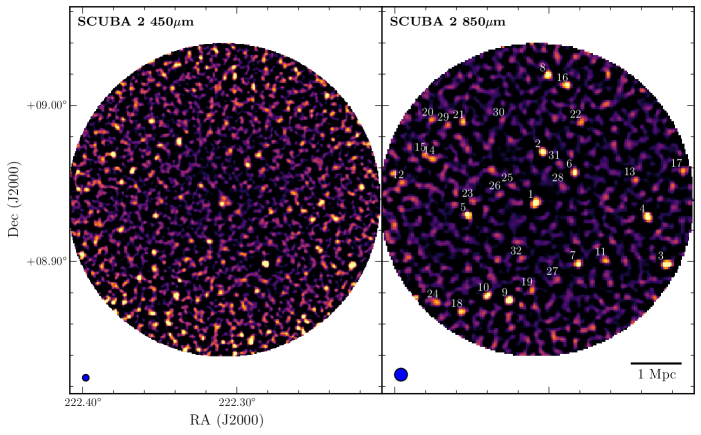
Figure 1: The SCUBA-2 maps of CLJ1449 with a radius of 3 Mpc. The FWHM size of the PSF can be found in the lower left corner. The positions of all 32 SCUBA-2 sources with a S/N greater than 4 are labeled on the 850 $\mu$m image, with the numbering being the same as that in Table 2

2.2 Herschel

To complement the SCUBA-2 data we have used publicly available data from both the Photoconductor Array Camera and Spectrometer (PACS, Poglitsch et al. 2010) and Spectral and Photometric Imaging Receive (SPIRE, Griffin et al. 2010). The PACS observations were acquired in July 2011 (ObsId 1342224474,1342224475, PI Gobat). Both 100 $\mu$m and 160 $\mu$m were observed over 10 hours in large scan map mode. The noise for these maps are 1.9 and 3.2 mJy and achieve a resolution of 7.7 arcsec and 12 arcsec for 100 and 160 $\mu$m respectively. All 3 SPIRE bands were observed with an integration time of 4 hours in January 2013 (ObsId 1342259448, PI Dannerbauer). The noise in the maps were 4.7, 5.5 and 6.2 mJy with a resolution of 18 arcsec, 26 arcsec and 36 arcsec for at 250, 350 and 500 $\mu$m respectively. Both the PACS and SPIRE level 2.5 data products were downloaded from the Herschel ESA archive.

2.3 ALMA

As part of cycle 1 the central area of the cluster was observed at 870 $\mu$m using ALMA (Project code 2012.1.00885.S, P.I Strazullo). The cluster was observed for 2.5 hours and only covers a small area (0.3 arcmin²). The map reaches a noise of 70 $\mu$Jy beam^-1 and has a resolution of $\sim$1 arcsec. For more information see C18. The data was acquired from the ALMA ESO science archive.

Even though the data only covers the central region of the cluster (see Figure 2), the higher resolution means that we will be able to detect confused source members that cannot be resolved in the SCUBA-2 images. This will be discussed further in Section 3.

2.4 JVLA - S Band

The S band radio data consist of observations from 2012 of JVLA S band (2-4GHz, project code: 12A-188, PI: V.Strazzullo.) using 16 spectral widows (128MHz bandwidth, 64 channels). The raw data was downloaded from the NRAO’s VLA archive, and each observation separately reduced using NRAO’s Astronomical Image Processing System (AIPS), following the standard VLA data calibration procedure described in the AIPS cookbook. For each observation, the calibrated UV data of the target field have been thoroughly flagged for radio-frequency interference and separated without averaging the frequency channels to avoid bandwidth smearing (chromatic aberrations). All of the resulting UV data sets have been combined for the final imaging, which consisted of a single phase-only and a final amplitude-and-phase calibration.

2.5 Spitzer

Complimentary IR data of CLJ1449 was obtained with Spitzer’s Infrared Array Camera (IRAC, Fazio et al. 2004). All 4 bands (3.6, 4.5, 5.8, and 8 $\mu$m, PI Giovanni, ObsId 4393984) were observed and used. Each of the IRAC bands cover the same area (27 arcmin $\times$ 22 arcmin) but due to offset between arrays, only the 3.6 $\mu$m and 5.8 $\mu$m data cover the same area as that in the SCUBA-2 maps. As part of the Spitzer warm mission the cluster was re-observed at 3.6 $\mu$m and 4.5 $\mu$m (PI Gobat, ObsId 42576640) and when combined with the pre-existing data complete coverage of the cluster is achieved for 3 of the 4 bands.

2.6 Additional Data

We also utilise archival optical and NIR maps for CLJ1449. Deep $B$, $I$ and $z$ were taken with Suprime-cam (Miyazaki et al. 2002) on the Subaru telescope achieving 5 $\sigma$ magnitudes depths of 26.95, 26.03 and 25.91 respectively. We also have NIR data ($Y$, $H$, $J$ and $Ks$) taken with both the Multi-Object Infrared Camera and Spectrograph (MOIRCS, Ichikawa et al. 2006, Suzuki et al. 2008) on Subaru and the Infrared Spectrometer And Array Camera (ISAAC, Moorwood et al. 1998) on the Very Large Telescope (VLT). These images reach depths at 5 $\sigma$ of 25.64, 25.47, 23.66 and 24.74 for $Y$, $H$, $J$ and $Ks$ respectively. Finally we have $U$ and $V$ band data taken with the FOcal Reducer and low dispersion Spectrograph (FORS, Appenzeller et al. 1998) also on the VLT, reaching 5 $\sigma$ depths of 28.1 and 26.52 for $U$ and $V$. For more information on these data sets we refer to Kong et al. (2006), Gobat et al. (2011) and Strazzullo et al. (2013). A summary of all data used in this analysis can be found in Table 1, and the fields of view (FOV) for all the maps used can be found in Figure 2.

Table 1: Summary of the data-sets used in our analysis.

Telescope	Instrument	Observed Band	FOV
VLT	FORS 2	U, V	7 arcmin $\times$ 7 arcmin
Subaru	Suprime	B,I,z	27 arcmin $\times$ 35 arcmin
Subaru	MOIRCS	Y,H	7 arcmin $\times$ 4 arcmin
VLT	ISAAC	J, Ks	7 arcmin $\times$ 4 arcmin
Spitzer	IRAC	3.6/4.5/5.8/8 $\mu$m	27 arcmin $\times$ 22 arcmin
Herschel	PACS	100/160 $\mu$m	15 arcmin $\times$ 15 arcmin
Herschel	SPIRE	250/350/500 $\mu$m	35 arcmin $\times$ 35 arcmin
JCMT	SCUBA-2	450/850 $\mu$m	113 arcmin2
ALMA	-	870 $\mu$m	0.3 arcmin2
JVLA	-	10 cm	20 arcmin $\times$ 20 arcmin

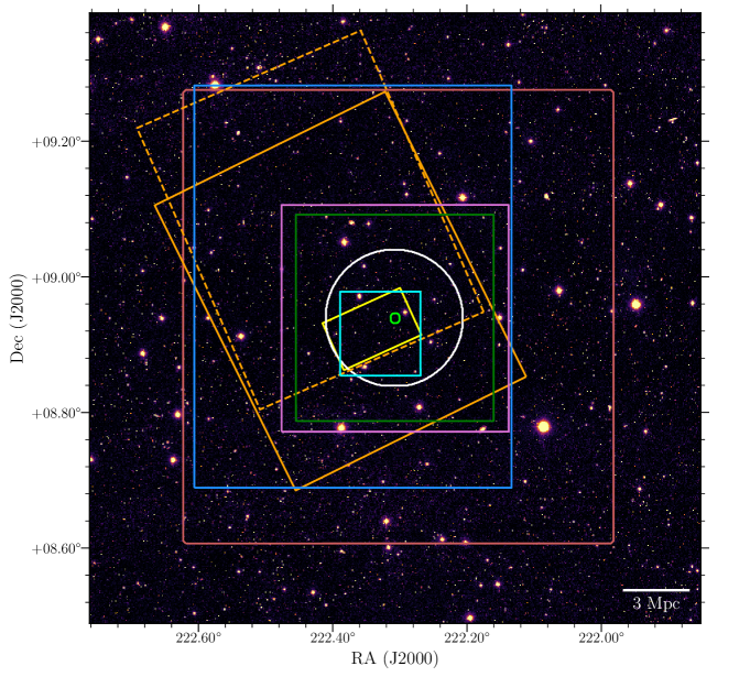
Figure 2: FOVs of all the data used in this analysis. The white circle represents the SCUBA-2 coverage (450/850 $\mu$m), whilst the small lime green circle represents the ALMA coverage. The yellow rectangle is the MOIRCS and ISAAC coverage (Y, H, J, and Ks bands), whilst the cyan square is the FORS 2 coverage (U and V band). The green square shows the PACS coverage (100/160 $\mu$m) and the purple square shows the radio data (10 cm). The solid orange rectangle shows the IRAC coverage at 3.6,4.6 and 5.8 $\mu$m, with the dashed orange rectangle showing the 8 $\mu$m coverage. The blue square shows the Suprime cam coverage (B, I and z bands) and the red square shows the SPIRE coverage (250/350/500 $\mu$m). The background is a g band image from SDSS.

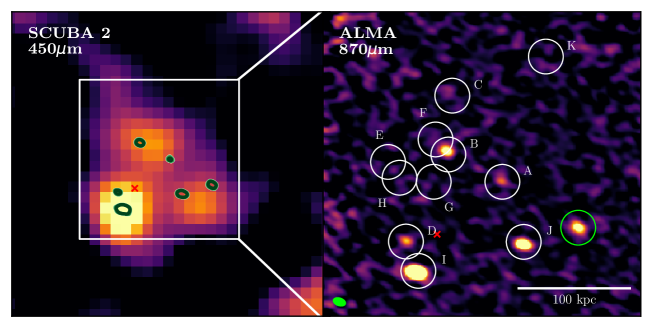
Figure 3: The ALMA 870 $\mu$m continuum map of the core of the cluster. The ALMA data resolves the SCUBA-2 450 $\mu$m map into 6 individual sources rather then 3. The size of the PSF can be see in the bottom left corner. The letter represents the sources in Table 3, and are based on the designations from C18. A low redshift object is known to contaminate the cluster, and is illustrated by the green circle. The red cross represents the centre of the x-ray emission from Gobat et al. 2011.

3 Source Identification

To identify any potential sub-mm sources we search for any sources in the SCUBA-2 850 $\mu$m map that have a signal to noise ratio (S/N) greater than 4. This uncertainty level was determined by inserting fake sources into a jackknife map, made by inverting half of the observations and co-adding. This produces a map with the same noise properties as the final map. Fake sources were then randomly inserted into the map (10⁵ sources inserted in batches of ten, with fluxes picked from a uniform distribution) and Sextractor (Bertin & Arnouts 1996) was then used to extract these sources.

It was found that with a S/N of 3.5 we are over 80% complete at $\sim$5 mJy. However the number of fake sources (i.e. sources caused entirely by noise) was very high, with there being 8 sources detected. At a S/N of 4 there was only 1 fake source, which is expected in a map of this size with Gaussian fluctuations. Therefore a S/N cut of 4 was selected.

In the SCUBA-2 850 $\mu$m map we detected 32 sources that have a S/N greater than 4, with the positions of all these sources given in Table 2, and their locations illustrated in Figure 1. When we looked at the 450 $\mu$m map we found that there were 18 sources with a S/N greater than 4. When cross matching these sources with the 850 $\mu$m ones we found only 11 sources matched. This low matching rate was also found by the SCUBA-2 Cosmology Legacy Survey (S2CLS). Casey et al. (2013) found that in the COSMOS field there was only a $\sim$30% matching rate when comparing 450 and 850 sources at the same S/N cut. This implies that the 450 $\mu$m population is intrinsically different than that of the 850 $\mu$m and indicates that different redshift or luminosity populations are being probed.

From the number counts of the S2CLS, in a field of the same size, at this sensitivity we would expect to see 10$\pm$3 sources at 850 $\mu$m (Geach et al. 2017). This means that our cluster field is more than three times over-dense.

Table 2: Catalogue of sources from the SCUBA-2 850 $\mu$m map that have a S/N greater than 4.

ID	RA	DEC	$r_{c}$	S/N850	S/N450
			(Mpc)
850_1	222.30882	8.93770	0.0	10.6	7.7
850_2	222.30423	8.97015	0.958	9.8	4.0
850_3	222.22436	8.89832	2.864	8.8	6.0
850_4	222.23642	8.92864	2.229	8.1	3.5
850_5	222.35272	8.92960	1.392	8.0	6.6
850_6	222.28385	8.95749	0.938	7.8	3.4
850_7	222.28147	8.89870	1.489	7.4	10.8
850_8	222.30102	9.01891	2.456	6.6	3.5
850_9	222.32561	8.87515	2.033	6.5	3.1
850_10	222.33980	8.87835	2.100	5.7	5.6
850_11	222.26360	8.90100	1.803	5.3	<2
850_12	222.39497	8.95028	2.679	5.0	<2
850_13	222.24476	8.95221	1.990	4.9	2.5
850_14	222.37475	8.96610	2.198	4.9	<2
850_15	222.38069	8.96798	2.389	4.8	6.8
850_16	222.28853	9.01256	2.331	4.8	4.4
850_17	222.21441	8.95775	2.937	4.8	2.6
850_18	222.35692	8.86788	2.646	4.8	3.6
850_19	222.31144	8.88167	1.766	4.7	3.0
850_20	222.37582	8.99054	2.602	4.5	2.9
850_21	222.35558	8.98888	2.104	4.4	5.0
850_22	222.27984	8.98906	1.762	4.3	<2
850_23	222.34994	8.93833	1.276	4.3	2.8
850_24	222.37243	8.87388	2.806	4.3	2.9
850_25	222.32408	8.94833	0.558	4.3	5.1
850_26	222.33233	8.94313	0.746	4.2	2.2
850_27	222.29483	8.88833	1.613	4.2	3.3
850_28	222.29146	8.94833	0.589	4.1	2.8
850_29	222.36570	8.98721	2.295	4.1	<2
850_30	222.32970	8.99055	1.707	4.1	<2
850_31	222.29371	8.96277	0.851	4.0	6.0
850_32	222.31845	8.90166	1.191	4.0	2.6

3.1 Source Confusion

Due to the large beam size of our SCUBA-2 data, assigning optical and NIR counterparts is difficult as several galaxies could be residing in one beam. An example of this can be seen with the SCUBA-2 images in Figure 1. In the 850 $\mu$m map (beam size 15 arcsec) the central region is seen as one source, but the 450 $\mu$m (beam size 8 arcsec) shows this one source resolved into 3 separate sources. The severity of this issue is fully realised when we compare the SCUBA-2 data to the ALMA 870 $\mu$m data, with a resolution of $\sim$1 arcsec. Figure 3 shows that the 3 sources in the 450 $\mu$m data actually is 6 individual sources, and this is only seen due to the high resolution of ALMA. It should be noted that C18 actually identify 11 galaxies within the central 200 kpc based on the positions of CO(4-3) detections.

Due to the large beam sizes of both SCUBA-2 and Hershcel there is a high probability that several sources may be blended into one individual source. This makes associating the FIR/sub-mm sources to optical and NIR sources complicated, as we do not know which optical and NIR sources are associated with the FIR/sub-mm ones.

3.2 De-Blending Sub-mm Images

To de-blend our images and get accurate flux measurements we used the Bayesian inference tool XID+ (Hurley et al. 2017). XID+ uses the positional data from a tracer of dusty star formation and explores the full posterior function to extract fluxes from confused maps. To assure the most accurate results from XID+, high resolution positional data is required from a wavelength that traces dust obscured star formation. For the central region we use the ALMA map and the 11 sources detected at 870 $\mu$m by C18. We also included the lower right source (circled green in Figure 3) even though this is a known low redshift object. This is because we need it for the de-blending process, but it is excluded from the rest of the analysis.

For the rest of the region, we had to use a different tracer. Good examples are either 24 $\mu$m (e.g. Marsden et al. 2009, Pascale et al. 2009, Elbaz et al. 2010, Béthermin et al. 2012) or radio (e.g. Ivison et al. 2010, Magnelli et al. 2010, Basu et al. 2015, Rujopakarn et al. 2016, Delhaize et al. 2017). Even though a MIPS 24 $\mu$m map was available, the beam size is still large ($\sim$6 arcsec) and galaxies will still be blended. Instead we used the 10 cm (3 GHz) JVLA map as our tracer, as it has resolution comparable to that of our ALMA map.

We identified 319 significant sources in the radio map (within the same area of the SCUBA-2 maps), and combine these with the 12 ALMA sources. These sources were then passed through XID+ to obtain fluxes for both the PACS and SPIRE maps. A specially modified version of XID+ was used to work with the SCUBA-2 maps, so we also have de-blended fluxes for both 450 $\mu$m and 850 $\mu$m.

3.3 Association With Radio Sources

We then went about associating each of our SCUBA-2 sources with at least one radio source (and therefore can associate with optical and NIR sources). To determine the most likely radio source we use the standard Poissonian probability of positional match similar to the method outlined in Downes et al. (1986). This value $P$ gives us the probability of a source not being associated with the SCUBA-2 source and is given by

$$P=1-\exp{(-\pi\,n\,\theta^{2})},$$ (1)

where $n$ is the number density of sources in the radio map, and $\theta$ is the separation between the SCUBA-2 source and the radio source. We found all radio sources within 15 arcsec of the SCUBA-2 source, and calculated the $P$ value for all of them. For galaxies that had similar $P$ values we picked the source that was reddest in the IRAC bands, as it has been shown that sub-mm galaxies tend to be redder at these wavelengths (e.g. Ashby et al. 2006, Yun et al. 2008, Hainline et al. 2009). We did not worry about the central source (source 850_1) as we use the ALMA sources from C18, which have been shown to have association with optical and NIR sources.

Using the prescriptions laid out in Ivison et al. (2002), Chapin et al. (2009) and Chen et al. (2016), we considered a reliable match to have a $P$ $\leq$ 0.05 and a tentative match to have 0.05$\leq P\leq$0.1. Anything with a $P>$0.1 is considered an untrustworthy match and removed. We found that all but 2 sources had either reliable or tentative matches, with 850_12 and 850_19 having sources too far to be considered significant. Even though 850_18 and 850_28 had low $P$ values, in the optical and NIR images they were obscured by nearby stars and hence removed from the sample. Finally 850_30 was removed because there was no radio source within 15 arcsec. Applying these cuts we ended up with 37 sources that we can calculate redshifts for, and determine if they are likely to be within the cluster or not.

4 Redshift Determination

To assign cluster membership we estimated redshifts for our remaining 37 galaxies, and those that had a redshift consistent with the cluster were considered members. However due to a lack of spectral data beyond the core region, we have to rely on photometric methods to determine the redshift for our sources. We performed aperture photometry on the optical and NIR maps (based on the radio positions), and accounted for difference in resolutions by applying aperture corrections. The maps were also calibrated by using stars of known brightness. This resulted in a 13 band catalogue spanning from U band ($\sim$ 0.3 $\mu$m) to 8 $\mu$m. However due to differing map sizes, only 6 bands (B, z, I, 3.6, 4.5 and 5.8 $\mu$m) had the same coverage as the SCUBA-2 maps, meaning our catalogue is incomplete (especially at NIR wavelengths).

4.1 Photometric Redshifts Using Optical and NIR Data

To calculate our photometric redshifts we first used the template fitting code EAZY using the standard set of templates (Brammer et al. 2008, 2011, Whitaker et al. 2011). We can see an example of the fit from EAZY in Figure 4, whilst Figure 5 shows the distribution of redshifts calculated with EAZY.

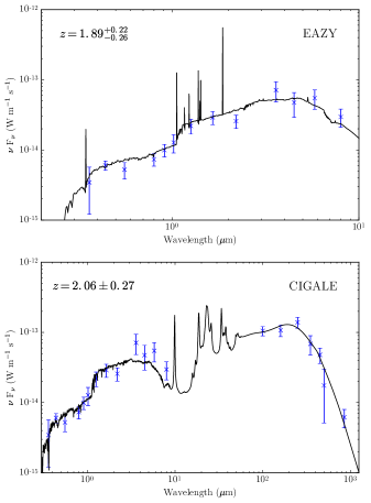
Figure 4: Both the EAZY SED (top) and CIGALE SED (bottom) for source 850_25

Figure 5: The photometric redshift distributions for both EAZY and CIGALE.

The main issue when using EAZY is our incomplete catalogue. Whilst EAZY gives accurate results in areas with complete data, such as in the cluster centre (with $\Delta$z being on average $\sim$ 0.2), in regions where there is no NIR data and just the Subaru and Spitzer data, $\Delta$z on average is $\sim$ 1 removing any precision needed in identifying cluster members. Using the optical and NIR data on its own is therefore not the most ideal situation, so we also looked at methods that included FIR/sub-mm data.

4.2 Photometric Redshifts Including Sub-mm Data

Using FIR/sub-mm data to estimate photometric redshifts has been studied several times (e.g. Pearson et al. 2013, Ivison et al. 2016, Bakx et al. 2018) and is ideal for situations where there is little or no optical and NIR counterparts to the sub-mm sources. However, these results can have significant uncertainties ($\pm$0.5 in some cases), and on their own would not have the accuracy to place them within the cluster. This is especially true with XID+, as areas where several sources exist (such as the centre) the errors on the fluxes are significant (up to 50% in some cases).

To calculate photometric redshifts using both optical, NIR, FIR and sub-mm data we use The Code Investigating GALaxy Emission (CIGALE, Boquien et al. 2018). CIGALE is a dust energy balancing code, which balances any energy lost via dust attenuation to that of the emission caused by the dust. This approach is more advantageous as even with a small/incomplete optical data set, reasonably accurate results can be estimated as long as the FIR/sub-mm data is complete. The main advantage of CIGALE over similar codes is the ability to leave redshift as a free parameter, and compute photometric redshifts from the full wavelength range.

Another advantage of CIGALE is the flexibility in models that can be selected. With CIGALE the user can determine the models and parameters used (e.g. what dust emission model is used, what star formation history, etc) which allows for greater variability. We decided to use the same parameters used in the Herschel Extragalactic Legacy Project (HELP, Vaccari 2016). These parameters were selected as they cover a wide range of models and suitable for most galaxy types, and include a delayed star formation history (with additional burst), single stellar population models from Bruzual & Charlot (2003), dust attenuation from Charlot & Fall (2000) and a Draine & Li (2007) dust emission model. For more information see Małek et al. (2018).

CIGALE was run for our 37 galaxies using the HELP settings, except for redshift which was kept as a free parameter. With the added data we found that the uncertainties were smaller, especially for those galaxies that had significant uncertainties with EAZY. Again an example of a fit generated from CIGALE can be seen in Figure 4 and distribution of redshifts can be seen in Figure 5. Comparisons between all three redshifts measures can be seen in Figure 6.

4.3 Cluster Membership

To determine the cluster membership we compared the photometric values to the values of those sources with spectral redshifts (Figure 6). The only sources that had spectral redshifts are nine of the central ALMA sources discussed in C18. To determine a range of redshifts that could indicate membership, we compared the scatter between the photometric and spectroscopic redshifts. We found that for both CIGALE and EAZY the scatter was $\sim 0.2$. Therefore it was decided that all galaxies within 2$\sigma$ of this scatter was considered a possible cluster member (i.e. any galaxy with a redshift between 1.6 and 2.4 is considered to be potentially in the cluster).

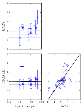
Figure 6: Comparing all three redshift determination methods. The black point shows the median value for both CIGALE, EAZY and errors.

We use a combination of both the EAZY and CIGALE redshifts to help determine cluster memberships. Based on these redshifts we decided on 3 categories of cluster membership, with the first having the highest probability of being in the cluster. These galaxies either have a spectroscopic redshift or meet our redshift cut in both the EAZY and CIGALE redshifts. The second category are galaxies that have a much less chance of actually being a cluster member. These are galaxies that have a redshift matching our cut in either EAZY or CIGALE. The final category is galaxies which are very likely to not be in the cluster, and do not have a redshift in EAZY or CIGALE. These galaxies are excluded from the rest of our analysis.

Applying this criteria we found that 16 galaxies have a high probability of being in the cluster, with nine of these having spectra and seven having redshifts confirmed by both EAZY and CIGALE. Eight galaxies have a tentative membership, with two only being confirmed by EAZY, and six only being confirmed by CIGALE. Overall we are left with 24 galaxies that could be cluster members with their fluxes being presented in Table 3, and the locations of them can be seen in Figure 7. A table of all non-cluster members can be found in Table 7.

We note that the number of galaxies that we exclude (14 galaxies) matches up well with the number of galaxies that we would expect to find in the field (Section 3, 10$\pm$3). This gives a greater confidence that the remaining galaxies are actually associated with the cluster.

Figure 7: Location of the final galaxies identified as possibly being within the cluster. It should be noted 850_1 actually consists of 10 members.

Table 3: FIR/sub-mm properties of our cluster galaxies.

ID	RA	DEC	$r_{c}$	$f_{100}$	$f_{160}$	$f_{250}$	$f_{350}$	$f_{450}$	$f_{500}$	$f_{850}$	Source
			(Mpc)	(mJy)	(mJy)	(mJy)	(mJy)	(mJy)	(mJy)	(mJy)
850_1_A	222.307	8.9395	0.04	0.26 $\pm$ 0.26	0.74 $\pm$ 0.73	10.26 $\pm$ 5.26	6.36 $\pm$ 5.99	1.12 $\pm$ 1.19	3.63 $\pm$ 3.76	0.81 $\pm$ 0.6	Spec
850_1_B	222.309	8.9403	0.04	0.31 $\pm$ 0.32	0.77 $\pm$ 0.83	1.66 $\pm$ 1.76	2.32 $\pm$ 2.51	1.06 $\pm$ 1.17	1.88 $\pm$ 2.15	0.47 $\pm$ 0.45	Spec
850_1_C	222.309	8.942	0.09	1.35 $\pm$ 0.59	2.41 $\pm$ 1.46	2 $\pm$ 1.84	1.22 $\pm$ 1.38	2.19 $\pm$ 1.72	1.24 $\pm$ 1.4	0.2 $\pm$ 0.22	Spec
850_1_D	222.31	8.9378	0.06	0.43 $\pm$ 0.39	0.7 $\pm$ 0.83	6.57 $\pm$ 5.26	6.74 $\pm$ 5.88	0.98 $\pm$ 1.09	4.03 $\pm$ 4.29	0.31 $\pm$ 0.37	Spec
850_1_E	222.31	8.9401	0.07	0.44 $\pm$ 0.37	0.72 $\pm$ 0.77	1.53 $\pm$ 1.71	2.01 $\pm$ 2.12	0.58 $\pm$ 0.64	1.61 $\pm$ 1.95	0.26 $\pm$ 0.29	Spec
850_1_F	222.309	8.9407	0.05	0.69 $\pm$ 0.53	1.49 $\pm$ 1.32	1.4 $\pm$ 1.64	1.85 $\pm$ 2.08	1.53 $\pm$ 1.47	1.61 $\pm$ 1.92	0.37 $\pm$ 0.36	Spec
850_1_G	222.309	8.9395	0.03	0.24 $\pm$ 0.26	0.42 $\pm$ 0.47	1.61 $\pm$ 1.76	3.48 $\pm$ 3.77	0.58 $\pm$ 0.69	2.51 $\pm$ 2.88	0.38 $\pm$ 0.39	Spec
850_1_H	222.31	8.9396	0.06	0.41 $\pm$ 0.37	0.68 $\pm$ 0.68	1.56 $\pm$ 1.71	1.86 $\pm$ 2.21	0.53 $\pm$ 0.58	1.75 $\pm$ 1.95	0.25 $\pm$ 0.26	Spec
850_1_K	222.306	8.9431	0.14	0.48 $\pm$ 0.36	2.51 $\pm$ 1.08	2.3 $\pm$ 1.91	1.16 $\pm$ 1.28	0.99 $\pm$ 0.94	1.06 $\pm$ 1.16	0.09 $\pm$ 0.1	Spec
850_13	222.244	8.9528	2.03	0.38 $\pm$ 0.33	1.85 $\pm$ 1.8	17.58 $\pm$ 4.18	12.48 $\pm$ 6.43	2.44 $\pm$ 1.87	6.24 $\pm$ 4.31	1.33 $\pm$ 0.96	Both
850_14	222.374	8.9664	2.19	3.79 $\pm$ 0.55	11.74 $\pm$ 1.26	21.31 $\pm$ 2.27	19.66 $\pm$ 2.99	2.04 $\pm$ 1.76	12.61 $\pm$ 4.17	4.31 $\pm$ 0.86	Both
850_17	222.216	8.9577	2.9	3.33 $\pm$ 0.55	4.57 $\pm$ 1.08	8.44 $\pm$ 2.4	3.36 $\pm$ 2.7	6.65 $\pm$ 3.21	1.42 $\pm$ 1.6	3.55 $\pm$ 0.92	Both
850_20	222.374	8.9911	2.57	5.73 $\pm$ 0.6	19.03 $\pm$ 1.43	36.86 $\pm$ 2.86	32.48 $\pm$ 3.75	5.45 $\pm$ 2.68	21.22 $\pm$ 4.56	2.57 $\pm$ 0.88	Both
850_22	222.28	8.9889	1.75	1.93 $\pm$ 0.74	2.39 $\pm$ 1.42	4.94 $\pm$ 3.34	5.89 $\pm$ 4.27	2.12 $\pm$ 1.8	4.23 $\pm$ 3.47	3.09 $\pm$ 1.29	Both
850_25	222.324	8.9485	0.55	3.5 $\pm$ 0.52	5.71 $\pm$ 1.07	11.58 $\pm$ 2.03	8.01 $\pm$ 2.46	7.19 $\pm$ 1.78	2.93 $\pm$ 2.07	1.75 $\pm$ 0.51	Both
850_31	222.292	8.9615	0.84	3.25 $\pm$ 0.52	8.44 $\pm$ 1.12	22.21 $\pm$ 2.28	18.13 $\pm$ 2.72	9.07 $\pm$ 1.92	11.05 $\pm$ 3.46	1.38 $\pm$ 0.5	Both
850_16	222.289	9.0128	2.33	10.75 $\pm$ 0.95	22.18 $\pm$ 2.92	10.83 $\pm$ 11.3	17.04 $\pm$ 12.56	3.24 $\pm$ 2.88	8.7 $\pm$ 6.94	1.58 $\pm$ 1.45	Ez
850_26	222.334	8.9446	0.8	2.28 $\pm$ 0.57	4.73 $\pm$ 1.31	1.6 $\pm$ 1.61	3.3 $\pm$ 3.36	1.54 $\pm$ 1.35	2.46 $\pm$ 2.47	0.93 $\pm$ 0.64	Ez
850_4	222.237	8.9284	2.23	0.39 $\pm$ 0.35	1.73 $\pm$ 1.03	6.55 $\pm$ 2.52	10.6 $\pm$ 3.89	7.88 $\pm$ 2.88	9.45 $\pm$ 4.46	5.48 $\pm$ 0.89	Cg
850_5	222.353	8.93	1.39	0.22 $\pm$ 0.23	3.17 $\pm$ 0.95	9.62 $\pm$ 2.12	14.42 $\pm$ 2.5	11.36 $\pm$ 2.35	15.63 $\pm$ 2.5	6.26 $\pm$ 0.8	Cg
850_8	222.301	9.0196	2.48	2.05 $\pm$ 0.54	2.8 $\pm$ 1.09	9.2 $\pm$ 2.13	12.06 $\pm$ 2.87	9.18 $\pm$ 2.98	10.01 $\pm$ 4.26	7.03 $\pm$ 1.05	Cg
850_9	222.326	8.8754	2.03	1.86 $\pm$ 0.53	14.04 $\pm$ 1.25	26.55 $\pm$ 2.34	34.25 $\pm$ 3.04	6.75 $\pm$ 2.85	23.96 $\pm$ 2.69	6.4 $\pm$ 0.99	Cg
850_24	222.373	8.8732	2.83	1.58 $\pm$ 0.56	7.94 $\pm$ 1.23	24.82 $\pm$ 2.36	31.12 $\pm$ 2.9	8.17 $\pm$ 3.5	25.21 $\pm$ 2.75	3.73 $\pm$ 1	Cg
850_1_J	222.306	8.9378	0.07	3.48 $\pm$ 0.56	10.98 $\pm$ 1.27	17.98 $\pm$ 4.51	19.58 $\pm$ 5.81	6.58 $\pm$ 1.91	12.57 $\pm$ 6.06	2.18 $\pm$ 0.64	Cg

4.4 Bright Cluster Core Sources

In C18 no spectral redshifts were detected for sources 850_1_I and 850_1_J (A5 and A4 in C18). When we calculated photometric redshifts for them we found that 850_1_I was not placed in the cluster for either method, both indicating it had a redshift of $\sim$2.8. When we look at the other source, 850_1_J we see that indeed EAZY placed it well outside of the cluster (z$\sim$4.3) whereas CIGALE placed it within the cluster (Figure 8).

Combined 850_1_I and 850_1_J contribute 70% of the 870 $\mu$m flux for the cluster core, meaning that the chance of these galaxies being interlopers is extremely small. Based on 870 $\mu$m source counts from Karim et al. (2013) the chance of not being associated with the cluster is less than 4$\times$10^-5 (C18). Lensing is an unlikely cause to the high fluxes simply because the mass of the cluster halo is not enough to boost the fluxes to the observed levels. A full discussion on this is presented in both C18 and S18, who exclude both sources from there analysis. For the rest of our analysis we include 850_1_J as a potential member based on its CIGALE redshift. When appropriate we also consider the situation that this galaxy is not in the cluster. We should note that the errors on 850_1_I are substantial for both EAZY and CIGALE, with both having $\Delta z>1$. Whilst there is a chance it could be in the cluster the large error means we cannot say for sure, and therefore the source is excluded from the rest of the analysis.

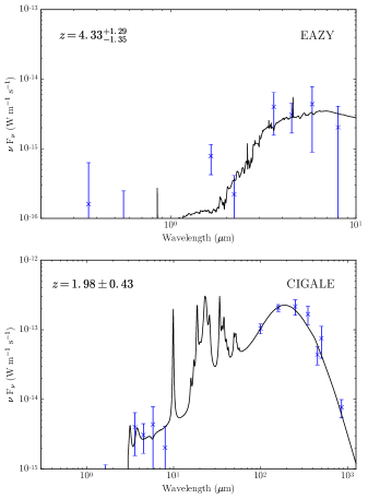
Figure 8: Comparing the SEDs from both EAZY and CIGALE for source 850_1_J. Notice that by including the sub-mm data the source is placed within the cluster

5 Star Forming Properties Of CLJ1449

With our list of cluster members we used CIGALE to fit SEDs for our analysis. Again the same settings as above were used, this time however the redshift was fixed at 2 for all galaxies. We used CIGALE rather then conventional methods of fitting a Modified Black-Body (MBB), because as mentioned the uncertainties on the FIR/sub-mm data are large, and we obtained better constraints using CIGALE. We find SFRs between 20-1600 M_⊙ yr^-1 with a median value of 168 M_⊙ yr^-1. The results from CIGALE can be found in Table 4, and all optical and NIR data can be found in Table 5 and 6.

Table 4: FIR/sub-mm properties of our cluster galaxies.

ID	$z_{Spec}$	$z_{EZ}$	$z_{CG}$	$L_{IR}$	$SFR$	$M_{*}$	$P$
				(1012 L⊙)	(M⊙yr-1)	(1011 M⊙)
850_1_A	1.9951 $\pm$ 0.0004	2.33${}^{+0.34}_{-0.31}$	2.25 $\pm$ 0.25	0.21 $\pm$ 0.15	32 $\pm$ 17	0.16 $\pm$ 0.08	-
850_1_B	1.9902 $\pm$ 0.0005	2.25${}^{+0.53}_{-0.55}$	2.14 $\pm$ 0.37	0.18 $\pm$ 0.22	22 $\pm$ 28	0.17 $\pm$ 0.21	-
850_1_C	1.9944 $\pm$ 0.0006	2.51${}^{+0.64}_{-0.87}$	1.92 $\pm$ 0.52	0.62 $\pm$ 0.38	74 $\pm$ 59	0.36 $\pm$ 0.17	-
850_1_D	1.9832 $\pm$ 0.0007	2.35${}^{+0.32}_{-0.28}$	1.70 $\pm$ 0.54	0.38 $\pm$ 0.10	36 $\pm$ 13	0.43 $\pm$ 0.13	-
850_1_E	1.9965 $\pm$ 0.0004	3.45${}^{+0.79}_{-0.70}$	2.23 $\pm$ 1.03	0.52 $\pm$ 0.48	66 $\pm$ 69	0.26 $\pm$ 0.37	-
850_1_F	1.9883 $\pm$ 0.0070	1.64${}^{+0.62}_{-0.66}$	2.02 $\pm$ 0.30	0.37 $\pm$ 0.30	45 $\pm$ 49	0.41 $\pm$ 0.22	-
850_1_G	1.9903 $\pm$0.0004	1.82${}^{+0.39}_{-0.47}$	1.59 $\pm$ 0.37	0.41 $\pm$ 0.37	59 $\pm$ 67	0.30 $\pm$ 0.29	-
850_1_H	1.982 $\pm$ 0.002	2.43${}^{+0.24}_{-0.24}$	3.62 $\pm$ 0.60	0.56 $\pm$ 0.67	73 $\pm$ 100	0.26 $\pm$ 0.44	-
850_1_K	1.98 $\pm$ 0.02	1.24${}^{+1.20}_{-0.83}$	1.63 $\pm$ 0.58	0.30 $\pm$ 0.11	37 $\pm$ 16	0.30 $\pm$ 0.12	-
850_13	-	1.98${}^{+0.44}_{-0.47}$	2.25 $\pm$ 0.24	0.94 $\pm$ 0.23	116 $\pm$ 22	2.08 $\pm$ 0.53	0.04
850_14	-	2.10${}^{+0.42}_{-0.47}$	1.79 $\pm$ 0.24	3.03 $\pm$ 0.36	331 $\pm$ 88	4.09 $\pm$ 0.99	0.01
850_17	-	2.34${}^{+0.87}_{-0.93}$	1.98 $\pm$ 0.40	3.65 $\pm$ 1.16	447 $\pm$ 156	3.86 $\pm$ 1.18	0.04
850_20	-	2.07${}^{+0.52}_{-0.51}$	2.04 $\pm$ 0.21	4.98 $\pm$ 0.38	439 $\pm$ 98	6.84 $\pm$ 1.48	0.08
850_22	-	2.35${}^{+0.43}_{-0.46}$	2.04 $\pm$ 0.32	3.30 $\pm$ 1.85	403 $\pm$ 214	2.28 $\pm$ 1.12	0.01
850_25	-	1.89${}^{+0.22}_{-0.26}$	2.06 $\pm$ 0.27	2.46 $\pm$ 0.44	254 $\pm$ 71	2.99 $\pm$ 0.83	0.01
850_31	-	2.18${}^{+0.77}_{-0.68}$	2.17 $\pm$ 0.32	2.73 $\pm$ 0.41	377 $\pm$ 117	1.33 $\pm$ 0.56	0.08
850_16	-	2.34${}^{+0.58}_{-0.57}$	1.56 $\pm$ 0.21	11.64 $\pm$ 2.71	1618 $\pm$ 738	7.25 $\pm$ 6.19	0.01
850_26	-	1.90${}^{+1.14}_{-0.86}$	1.26 $\pm$ 0.36	2.35 $\pm$ 0.98	313 $\pm$ 160	0.74 $\pm$ 0.52	0.09
850_4	-	1.56${}^{+0.92}_{-0.97}$	1.96 $\pm$ 0.34	0.93 $\pm$ 0.18	105 $\pm$ 30	0.58 $\pm$ 0.39	0.002
850_5	-	1.46${}^{+0.87}_{-0.78}$	1.98 $\pm$ 0.70	1.26 $\pm$ 0.14	142 $\pm$ 40	0.61 $\pm$ 0.32	0.004
850_8	-	1.58${}^{+0.49}_{-0.41}$	2.10 $\pm$ 0.97	1.71 $\pm$ 0.28	195 $\pm$ 63	0.74 $\pm$ 0.49	0.01
850_9	-	3.52${}^{+0.35}_{-0.36}$	2.07 $\pm$ 0.39	3.55 $\pm$ 0.27	357 $\pm$ 86	2.51 $\pm$ 1.22	0.002
850_24	-	2.61${}^{+0.60}_{-0.56}$	2.27 $\pm$ 0.39	2.99 $\pm$ 0.34	360 $\pm$ 101	1.67 $\pm$ 0.64	0.01
850_1_J	-	4.33${}^{+1.29}_{-1.35}$	1.98 $\pm$ 0.43	2.98 $\pm$ 0.28	381 $\pm$ 138	1.31 $\pm$ 1.33	-

5.1 Radial Variations In The Star Formation Rate Density

To understand the radial variation in the SFR of the cluster, we calculated the distance from the centre for each galaxy and binned them in 0.5 Mpc bins ranging from 0-3 Mpc. We summed up the SFRs in each radial bin, and normalise it by the volume of the bin. The resulting plot can be seen in Figure 9.

We confirm that the central 0.5 Mpc region is highly star forming with a total SFR of 800 $\pm$ 200 M_⊙ yr^-1. When converted into a SFRD we find a projected volume density of (1.2 $\pm$ 0.3)$\times$10⁴ M_⊙yr^-1Mpc^-3, which is almost five orders of magnitude greater than the expected value for field galaxies ($\sim$0.1 M_⊙ yr^-1Mpc^-3, Madau & Dickinson 2014). With increasing radius we see a decrease in the SFRD of almost 2 orders of magnitude, until it stabilizes at 1 Mpc, where it remains constant with the exception of a spike between 2-2.5 Mpc. A similar spike was seen in Santos et al. (2014) in a redshift 1.6 cluster, and was caused by an increase in the number of high mass galaxies at this radius. This is again seen in CLJ1449 with the heaviest galaxy in our sample (850_16, M${}_{*}\sim$7.5 $\times$10¹¹ M_⊙) being found in this radius bin.

For completeness we also considered the scenario where 850_1_J is not associated with the cluster (the black star in the 0-0.5 Mpc bin in Figure 9). We find that the SFR for the central 0.5 Mpc region decreases to 440 $\pm$ 160 M_⊙ yr^-1 a factor of $\sim$ 2 lower then before. Again when converted to a SFRD this gives (6.7 $\pm$ 2.4)$\times$10³ M_⊙yr^-1Mpc^-3, which whilst lower then before, it is still much larger than the expected result from Madau & Dickinson (2014) for field galaxies.

In Figure 9 we also plot the number density of sources as a function of radius. Again we see an identical trend to what is observed with the SFR-density relation. This would indicate that the observed reversal in the SF-density relation is caused by a dense population of SF galaxies, rather then a small population of extreme starbursts.

We stress that the high number counts in the central 1 Mpc region is down to the high resolution ALMA data, whereas those counts at radii greater than 1 Mpc are based on radio sources. If we base our number counts entirely on the radio data then we find that the number density in the central region reduces by half. Whilst this is still a significant, it could indicate that we are not observing all the galaxies within the cluster.

The biggest issue with the galaxies beyond 1 Mpc is the redshift and their uncertainties. When doing the CIGALE fitting we fix the redshift to that of the cluster, so if we have an interloper this could cause an increase in the SFR. To test for this we normalise our SFR with the cosmological volume between 1.6 $<$z $<$2.4 for radii greater than 1 Mpc (as opposed to the cluster volume). When accounting for just the cosmological volume (Figure 9) the SF-density does indeed fall to expected field values at radii greater than 1 Mpc. This indicates that there is a high chance of significant contamination in our sample, which causes an artificial increase in the SF.

We do note that the two volumes we have normalised by are the two extreme cases. Using the cluster volume assumes all sources above 1 Mpc are in the cluster, and the cosmological volume assumes that none are. Whilst we do acknowledge that either one of these extremes could be occurring (no matter how unlikely), the fact that even at a radius greater than 1 Mpc we are still in a very over-dense region ($\sim$ 2 $\times$ over-dense) the chances are we are in the middle of these scenarios. This means we still expect elevation in the SF-density relation above the expected value, but it will not be as extreme as seen in Figure 9.

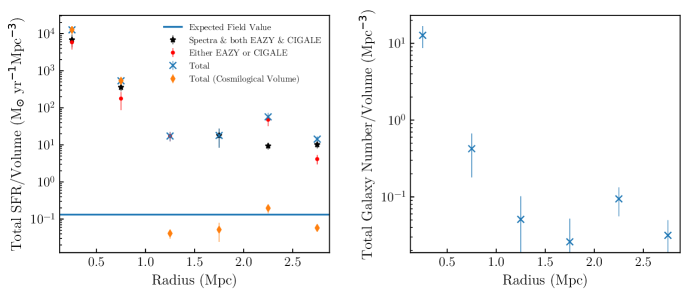
Figure 9: Left: The SF-density relation found in CLJ1449. We have divided the cluster into 0.5 Mpc bins, normalised by the volume of the bin. Each bin has been separated by the redshift criteria mentioned in Section 4. The blue line is the expected field value based on Madau & Dickinson (2014). We also plot the SF-density relation by assuming the observed cosmological volume between 1.6 $<$z $<$2.4. Right: The number density of galaxies versus the cluster radius. For sources less than 1 Mpc the counts are from ALMA, whilst at larger radii we use radio counts

5.2 Star Formation Rate vs Stellar Mass

We then investigated the relation between the stellar masses (M_∗) of our cluster galaxies and their SFRs. Using stellar masses from CIGALE we compare them to the SFRs, with the resulting relation shown in Figure 10. We compare these galaxies to the expected galaxy Main Sequence (MS) relation for redshift 2 galaxies from Sargent et al. (2014). Even though all these galaxies are highly star forming, and are extremely luminous (with all of them being LIRGs or ULIRGs) we find that the majority of galaxies within the cluster do not deviate from the expected main sequence. This behaviour was observed by C18 when observing the central galaxies. However they noted that these galaxies had star-burst like behaviour, based on the gas excitation.
Figure 10 would seem to suggest that the environment does not have a significant effect on the SF properties of these galaxies. Darvish et al. (2016) found that in the COSMOS field, galaxies at low redshift (z $<$ 1) seemed to be heavily influenced by the environment they reside in, and in dense environments the SFR decreased significantly. However at z $>$ 1 the SFR did not significantly change with environment, suggesting that at high redshift the SFR-M_∗ relation is independent of environment. This behaviour was also seen by Koyama et al. (2013) who again suggest the SFR-M_∗ relation is not dependant on the galaxy environment at high redshift.
We can link the low level of starbursts back to the density of sources seen in Figure 9. If we had a low number density of sources in the cluster core, we would expect to see far more galaxies exhibiting star burst behaviour to account for the large SF-density. The fact that we have a high number density of sources in the cluster core and limited starbursts reinforce the claim that the SFR-density relation is caused by a high density of SF galaxies sources rather than a small population of star bursting galaxies.
A small sample of our galaxies do appear to lie above the MS, being $\sim$2-3 $\times$ above the expected relation. This enhanced SF activity could indeed be down to merging events, as both Hung et al. (2013) and Cibinel et al. (2018) found that galaxies undergoing a merging event lie above the galaxy MS. This would also validate claims made by C18 that most of the activity in this cluster is driven by mergers. It should be noted that these galaxies that are above the main sequence are those galaxies that had their redshifts estimated by either EAZY or CIGALE. As mentioned earlier this increase in SF could be an artifact of fixing the redshift when running CIGALE.
Mergers could also explain why there is elevated SF (compared to the field) well beyond the viral radius of the cluster. Within the cluster core itself, galaxies are moving too fast for a merger to actually occur. However in the in-fall region the speed of galaxies is much lower allowing mergers to occur, and then be accreted onto the core (Bekki 1998, Moss 2006). Whilst measuring velocity dispersion is still very difficult at high redshift, Delahaye et al. 2017 showed evidence that the fraction of mergers in a redshift 1.6 cluster core is no higher than field values, indicating that the mergers are still happening in the outskirt rather than in the core itself. So in the outskirts of the clusters, mergers can occur more frequently and cause an increase in star formation. Whilst signs of merger activity cannot be detected with the current ground based optical data, it is hoped with new high resolution data this can be investigated further.
Whilst we have discussed the fact that environment and SF are independent at high redshift, it should be noted that in the left panel of Figure 10 the galaxies with the smallest cluster radii have the lowest stellar masses. This could suggest that the cluster environment is beginning to have an impact on the cluster galaxies, and quenching is starting to occur within these galaxies. Similar conclusions were drawn by both C18 observing this cluster, and Santos et al. 2014 observing a redshift 1.6 cluster.
In Figure 10 we convert our SFR to a specific SFR (sSFR, SFR/M_∗) and observe a large scatter from the proposed relation outlined in Sargent et al. (2014). Because the sSFR measures how the current SFR compares to to the SFR of the galaxy averaged over its life, the fact these galaxies have heightened sSFRs indicates that they are undergoing bursts of star formation.
A decrease in sSFR with increasing stellar mass has been reported at all redshifts (e.g. Ilbert et al. 2015, Lehnert et al. 2015) and is believed to show that the most massive galaxies have already formed all their stellar mass much earlier then their lighter counterparts. Whilst with this data suggests that there is a trend, it is not statistically significant enough to be considered, with a Spearman’s rank correlation coefficient of only -0.3. This could indicate that the heaviest galaxies are still in the process of forming within the cluster.

Figure 10: Left: The SFR-M_∗ relation with the shaded region showing the expected position for main sequence galaxies at redshift 2 given by Sargent et al. (2014). We have divided the points up into there location within the cluster and colour coded them accordingly. Right: The sSFR-M_∗ relation with the expected value for redshift 2 main sequence galaxies.

5.3 Mass Normalised Star Formation Rate

As we have discussed there is strong indication for an increase in the SF activity in clusters with increasing redshift. It has been shown that CLJ1449 is still very actively star forming but is this in line with what would be expected at this redshift. To allow for direct comparisons to other studies we follow the same methodology outlined in Popesso et al. (2012). We first integrate out to a radius of 1 Mpc (as in studies such as Santos et al. 2014 and Ma et al. 2015), giving a total integrated SFR ($\Sigma$SFR) of 1800 $\pm$ 300 M_⊙yr^-1. We then normalise $\Sigma$SFR by the cluster mass ((0.5$\pm$0.1) $\times$10¹⁴ M_⊙) resulting in a normalised, $\Sigma$SFR/M_cl of 3300 $\pm$ 850 M_⊙ yr^-1/10¹⁴ M_⊙.

In Figure 11 we compare our result to clusters at several different redshifts. We see that our cluster lies above the expected evolutionary trend predicted by Popesso, however this cluster is at a much higher redshift then their sample. When comparing the theorised (1+$z$)⁷ line in Cowie et al. (2004) and Geach et al. (2006), to CLJ1449 we see that there is only a 1.3 $\sigma$ offset, meaning that CLJ1449 could follow trends seen at both low and high redshift. When comparing to other high redshift (proto-)clusters from both Wang et al. (2016) (CLJ1001) and Casey (2016) we see that there is significant scatter. Other studies of proto-clusters such as those by Shimakawa et al. (2014) and Lacaille et al. (2018) has also showed significant scatter at z$\,>\,$2. This scatter was observed by Geach et al. (2006) at low redshift and suggests that the cluster environments have differing, but strong influences on the star formation histories of the residing galaxies. This is very significant for the sample from Casey (2016) which are proto-clusters, and are still in the process of forming.

It should also be noted that both CLJ1449 and CLJ1001 are significantly less massive then other clusters used in previous studies, both at low and high redshift. The fact that these clusters do not directly fit to the $(1+z)^{7}$ relation, and there is some scatter that could indicate cluster mass could have some influence on the galaxies within them. This was also suggested by both Koyama et al. (2011) and Cochrane et al. (2018) who observed similar scatter in z$\,>\,$1 clusters. Cluster mass and the SF properties of cluster galaxies will be investigated in future works. However for the time being high redshift samples are still too small to determine if all clusters have enhanced SF activity, or do they behave like low redshift galaxies and we have a biased sample.

Figure 11: Comparison of the mass normalised $\Sigma$SFR for several clusters at different redshifts. The solid black line is the proposed relation offered by Cowie et al. (2004) and Geach et al. (2006) that follows the relation $(1+z)^{7}$, and the blue dashed line follows the relation in Popesso et al. (2012) for clusters. It should be noted that the sample from Casey (2016) are proto-clusters and not fully virialized clusters.

6 Conclusions

We have presented new SCUBA-2 images of CLJ1449, a mature cluster at redshift two. We combine this data with pre-existing data including Herschel, ALMA and VLA to study the SF properties of this cluster, and build upon the work already presented in C18 and S18.

• We use SCUBA-2 and Herschel data to explore $\sim$0.03 deg² that contain the cluster CLJ1449. We identify 32 sources in the 850 $\mu$m maps that have a S/N greater then 4.

• To help estimate fluxes for confused members we use high resolution ALMA and JVLA maps to identify positions of potential FIR/sub-mm galaxies. We then use the Bayesian inference tool XID+ to estimate fluxes for all these sources in the confused Herschel and SCUBA-2 maps.

• We match these sources up to our SCUBA-2 sources resulting in 37 potential cluster members. To confirm cluster membership we calculate redshifts using both EAZY and CIGALE. We find 24 galaxies we are confident could be within the cluster.

• We use CIGALE estimates for both SFRs and stellar masses for all 24 galaxies. We find that the central 0.5 Mpc region is very highly star forming, forming 800$\pm$200 M_⊙yr^-1, which corresponds to a SFRD of (1.2 $\pm$ 0.3)$\times$10⁴ M_⊙yr^-1Mpc^-3. This is orders of magnitude greater then field values.

• When looking at the SFR-M_∗ relation we see these galaxies lie on the expected main sequence relation, however there is some evidence of star-bursting activity which could possibly be caused by merger events. When looking at the sSFR-M_∗ we see a large scatter in this relation which could indicate that the gas is undergoing complex processes.

• When comparing the mass normalised integrated SFR we see that CLJ1449 seems to follow previously identified scaling relations (with minimal scatter), but there is still a large scatter when considering other high redshift systems. However due to the low number of high redshift systems it is unknown if this is reflective of what is seen in low redshift systems.

Appendix A Optical and NIR Data For Cluster Members

Table 5: Optical and NIR data of our cluster galaxies. The units are in $\mu$Jy.

ID	U	B	V	I	Z	Y
850_1_A	0.45 $\pm$ 0.28	1.32 $\pm$ 0.2	1.25 $\pm$ 0.31	0.07 $\pm$ 0.22	1.15 $\pm$ 0.23	0.75 $\pm$ 0.41
850_1_B	0.06 $\pm$ 0.1	0.14 $\pm$ 0.02	0.1 $\pm$ 0.07	0.21 $\pm$ 0.04	0.2 $\pm$ 0.04	0.16 $\pm$ 0.18
850_1_C	0.11 $\pm$ 0.14	0.06 $\pm$ 0.01	0.13 $\pm$ 0.08	0.33 $\pm$ 0.07	0.4 $\pm$ 0.08	0.33 $\pm$ 0.26
850_1_D	0.01 $\pm$ 0.05	-	-	-	0.06 $\pm$ 0.01	0.22 $\pm$ 0.21
850_1_E	0.02 $\pm$ 0.06	-	0.08 $\pm$ 0.06	0.13 $\pm$ 0.03	0.19 $\pm$ 0.04	0.07 $\pm$ 0.12
850_1_F	0.18 $\pm$ 0.18	0.33 $\pm$ 0.05	0.21 $\pm$ 0.1	0.54 $\pm$ 0.11	0.77 $\pm$ 0.15	0.56 $\pm$ 0.34
850_1_G	0.06 $\pm$ 0.1	0.16 $\pm$ 0.02	-	0.14 $\pm$ 0.03	0.54 $\pm$ 0.11	-
850_1_H	0.02 $\pm$ 0.05	0.09 $\pm$ 0.01	0.05 $\pm$ 0.05	-	0.05 $\pm$ 0.01	0.1 $\pm$ 0.14
850_1_K	-	0.25 $\pm$ 0.04	-	0.72 $\pm$ 0.14	2.16 $\pm$ 0.43	0.7 $\pm$ 0.39
850_13	-	3.19 $\pm$0.48	-	2.81 $\pm$ 0.56	4.57 $\pm$ 0.91	-
850_14	1.73 $\pm$ 0.59	2.61 $\pm$ 0.4	2.16 $\pm$ 0.45	2.87 $\pm$ 0.57	4.99 $\pm$ 1.0	-
850_17	-	2.98 $\pm$ 0.45	-	8.14 $\pm$ 1.63	12.96 $\pm$ 2.59	-
850_20	-	0.35 $\pm$ 0.05	-	0.8 $\pm$ 0.16	1.45 $\pm$ 0.29	-
850_22	-	7.32 $\pm$ 1.1	-	5.84 $\pm$ 1.17	8.24 $\pm$ 1.65	-
850_25	0.41 $\pm$ 0.27	0.89 $\pm$ 0.13	0.97 $\pm$ 0.26	1.96 $\pm$ 0.39	3.02 $\pm$ 0.6	4.33 $\pm$ 1.25
850_31	-	0.08 $\pm$ 0.01	0.13 $\pm$ 0.08	-	0.68 $\pm$ 0.14	0.46 $\pm$ 0.31
850_16	-	2.08 $\pm$ 0.31	-	2.89 $\pm$ 0.58	5.13 $\pm$ 1.03	-
850_26	-	0.56 $\pm$ 0.08	-	1.18 $\pm$ 0.24	2.56 $\pm$ 0.51	-
850_4	-	0.81 $\pm$ 0.12	-	0.87 $\pm$ 0.17	1.05 $\pm$ 0.21	-
850_5	-	0.42 $\pm$ 0.06	-	0.49 $\pm$ 0.1	0.76 $\pm$ 0.15	-
850_8	-	0.46 $\pm$ 0.07	-	0.33 $\pm$ 0.07	0.95 $\pm$ 0.19	-
850_9	0.04 $\pm$ 0.08	0.04 $\pm$ 0.01	0.2 $\pm$ 0.1	0.47 $\pm$ 0.09	0.84 $\pm$ 0.17	0.41 $\pm$ 0.29
850_24	0.08 $\pm$ 0.12	0.43 $\pm$ 0.07	-	1.16 $\pm$ 0.23	1.43 $\pm$ 0.29	-
850_1_J	0.02 $\pm$ 0.06	-	0.02 $\pm$ 0.03	-	-	-

Table 6: NIR and MIR data for our cluster galaxies. The units are in $\mu$Jy.

ID	J	H	K	3.6 $\mu$m	4.8 $\mu$m	5.8 $\mu$m	8 $\mu$m
850_1_A	1.68 $\pm$ 0.6	2.57 $\pm$ 0.68	3.72 $\pm$ 0.98	6.92 $\pm$ 4.34	9.59 $\pm$ 5.05	6.16 $\pm$ 6.36	6.77 $\pm$ 6.26
850_1_B	0.16 $\pm$ 0.18	0.56 $\pm$ 0.31	1.08 $\pm$ 0.36	2.94 $\pm$ 0.82	26.35 $\pm$ 16.39	-	-
850_1_C	1.15 $\pm$ 0.47	2.72 $\pm$ 0.71	3.39 $\pm$ 0.92	4.66 $\pm$ 3.15	6.72 $\pm$ 3.92	15.28 $\pm$ 12.91	15.59 $\pm$ 8.21
850_1_D	1.19 $\pm$ 0.48	2.54 $\pm$ 0.67	4.41 $\pm$ 1.13	9.31 $\pm$ 5.33	6.25 $\pm$ 4.27	14.27 $\pm$ 8.04	1.43 $\pm$ 4.74
850_1_E	0.15 $\pm$ 0.15	1.05 $\pm$ 0.35	1.65 $\pm$ 0.54	3.88 $\pm$ 2.81	11.54 $\pm$ 8.79	12.59 $\pm$ 8.08	23.9 $\pm$ 10.32
850_1_F	2.19 $\pm$ 0.72	3.67 $\pm$ 0.9	7.27 $\pm$ 1.71	-	-	-	-
850_1_G	1.1 $\pm$ 0.46	2.51 $\pm$ 0.66	2.58 $\pm$ 0.75	12.71 $\pm$ 7.9	21.75 $\pm$ 14.4	18.86 $\pm$ 10.62	18.39 $\pm$ 8.9
850_1_H	0.31 $\pm$ 0.22	1.13 $\pm$ 0.37	1.84 $\pm$ 0.58	7.46 $\pm$ 3.71	16.56 $\pm$ 9.36	19.43 $\pm$ 10.69	29.89 $\pm$ 16.48
850_1_K	2.02 $\pm$ 0.68	5.0 $\pm$ 1.17	7.46 $\pm$ 1.75	9.55 $\pm$ 7.71	4.43 $\pm$ 4.15	5.62 $\pm$ 5.84	4.61 $\pm$ 5.89
850_13	-	-	-	73.78 $\pm$ 24.98	93.43 $\pm$ 28.31	130 $\pm$ 39	78.39 $\pm$ 23.33
850_14	-	-	-	52.14 $\pm$ 14.9	78.91 $\pm$ 18.42	85.72 $\pm$ 22.91	107 $\pm$ 24
850_17	-	-	-	91.62 $\pm$ 33.41	112 $\pm$ 27	103 $\pm$ 25	110 $\pm$ 25
850_20	-	-	-	86.18 $\pm$ 27.08	137 $\pm$ 37	129 $\pm$ 40	76.1 $\pm$ 22.79
850_22	-	-	-	31.29 $\pm$ 10.45	56.36 $\pm$ 16.74	67.86 $\pm$ 23.89	140 $\pm$ 35
850_25	9.25 $\pm$ 2.18	15.96 $\pm$ 3.38	18.89 $\pm$ 4.05	85.41 $\pm$ 27.26	70.97 $\pm$ 27.49	105 $\pm$ 32	79.02 $\pm$ 22.71
850_31	2.63 $\pm$ 0.81	4.32 $\pm$ 1.03	8.59 $\pm$ 1.98	19.77 $\pm$ 10.58	14.54 $\pm$ 8.93	40.47 $\pm$ 19.89	34.77 $\pm$ 15.6
850_16	-	-	-	84.42 $\pm$ 26.66	117 $\pm$ 35	145.42 $\pm$ 49.35	166 $\pm$ 42
850_26	3.08 $\pm$ 0.91	5.71 $\pm$ 1.32	11.13 $\pm$ 2.49	29.33 $\pm$ 14.59	19.75 $\pm$ 12.12	36.97 $\pm$ 22.32	67.18 $\pm$ 33.45
850_4	-	-	-	-	-	-	-
850_5	-	-	1.8 $\pm$ 0.58	-	-	-	-
850_8	-	-	-	1.52 $\pm$ 1.54	7.59 $\pm$ 3.91	2.43 $\pm$ 8.95	1.86 $\pm$ 10.4
850_9	-	-	-	17.08 $\pm$ 6.34	49.19 $\pm$ 14.08	63.37 $\pm$ 21.07	-
850_24	-	-	-	31.74 $\pm$ 8.33	29.72 $\pm$ 9.43	37.5 $\pm$ 13.05	-
850_1_J	-	0.43 $\pm$ 0.2	0.16 $\pm$ 0.14	4.8 $\pm$ 2.92	4.62 $\pm$ 2.1	8.44 $\pm$ 6.71	5.4 $\pm$ 5.51

Appendix B Redshifts For All Non-Cluster Members

Table 7: Redshifts for the non-cluster members.

ID	RA	DEC	$z_{EZ}$	$z_{CG}$
850_1_I	222.309	8.936	2.48${}^{+0.72}_{-1.18}$	2.41$\pm$1.21
850_2	222.304	8.970	2.92${}^{+0.49}_{-0.54}$	3.77$\pm$0.74
850_3	222.225	8.897	2.59${}^{+0.81}_{-1.06}$	1.44$\pm$0.56
850_6	222.284	8.957	2.57${}^{+0.33}_{0.34}$	3.95$\pm$0.50
850_7	222.281	8.899	1.27${}^{+0.29}_{-0.30}$	1.46$\pm$0.35
850_10	222.340	8.878	2.40${}^{+0.75}_{-0.76}$	3.01$\pm$0.64
850_11	222.263	8.901	3.14${}^{+0.62}_{-0.61}$	3.70$\pm$0.56
850_15	222.380	8.968	0.94${}^{+0.46}_{-0.46}$	0.97$\pm$0.30
850_21	222.355	8.990	2.83${}^{+0.67}_{-0.64}$	3.25$\pm$0.58
850_23	222.348	8.937	0.14${}^{+0.07}_{-0.09}$	1.27$\pm$1.31
850_27	222.295	8.889	2.59${}^{+0.43}_{-0.63}$	2.43$\pm$0.35
850_29	222.363	8.988	1.51${}^{+0.55}_{-0.47}$	1.44$\pm$0.24
850_32	222.317	8.902	1.46${}^{+0.23}_{-0.22}$	1.50$\pm$0.18

References

- Alexander et al. (2016) Alexander D. M., et al., 2016, MNRAS, 461, 2944
- Andreon et al. (2014) Andreon S., Newman A. B., Trinchieri G., Raichoor A., Ellis R. S., Treu T., 2014, A&A, 565, A120
- Appenzeller et al. (1998) Appenzeller I., et al., 1998, The Messenger, 94, 1
- Ashby et al. (2006) Ashby M., et al., 2006, in American Astronomical Society Meeting Abstracts 208. p. 145
- Astropy Collaboration et al. (2013) Astropy Collaboration et al., 2013, A&A, 558, A33
- Bakx et al. (2018) Bakx T. J. L. C., et al., 2018, MNRAS, 473, 1751
- Baldry et al. (2006) Baldry I. K., Balogh M. L., Bower R. G., Glazebrook K., Nichol R. C., Bamford S. P., Budavari T., 2006, MNRAS, 373, 469
- Basu et al. (2015) Basu A., Wadadekar Y., Beelen A., Singh V., Archana K. N., Sirothia S., Ishwara-Chandra C. H., 2015, ApJ, 803, 51
- Bekki (1998) Bekki K., 1998, ApJ, 502, L133
- Bertin & Arnouts (1996) Bertin E., Arnouts S., 1996, A&AS, 117, 393
- Béthermin et al. (2012) Béthermin M., et al., 2012, A&A, 542, A58
- Bleem et al. (2015) Bleem L. E., et al., 2015, ApJS, 216, 27
- Boquien et al. (2018) Boquien M., Burgarella D., Roehlly Y., Buat V., Ciesla L., Corre D., Inoue A. K., Salas H., 2018, preprint, (arXiv:1811.03094)
- Brammer et al. (2008) Brammer G. B., van Dokkum P. G., Coppi P., 2008, ApJ, 686, 1503
- Brammer et al. (2011) Brammer G. B., et al., 2011, ApJ, 739, 24
- Bruzual & Charlot (2003) Bruzual G., Charlot S., 2003, MNRAS, 344, 1000
- Cai et al. (2017) Cai Z., et al., 2017, ApJ, 839, 131
- Calzetti et al. (2007) Calzetti D., et al., 2007, ApJ, 666, 870
- Casasola et al. (2018) Casasola V., et al., 2018, preprint, (arXiv:1806.09493)
- Casey (2016) Casey C. M., 2016, ApJ, 824, 36
- Casey et al. (2013) Casey C. M., et al., 2013, MNRAS, 436, 1919
- Chapin et al. (2009) Chapin E. L., et al., 2009, MNRAS, 398, 1793
- Chapin et al. (2013) Chapin E. L., Berry D. S., Gibb A. G., Jenness T., Scott D., Tilanus R. P. J., Economou F., Holland W. S., 2013, MNRAS, 430, 2545
- Charlot & Fall (2000) Charlot S., Fall S. M., 2000, ApJ, 539, 718
- Chen et al. (2016) Chen C.-C., et al., 2016, ApJ, 820, 82
- Chiang et al. (2013) Chiang Y.-K., Overzier R., Gebhardt K., 2013, ApJ, 779, 127
- Chiang et al. (2017) Chiang Y.-K., Overzier R. A., Gebhardt K., Henriques B., 2017, ApJ, 844, L23
- Cibinel et al. (2018) Cibinel A., et al., 2018, preprint, (arXiv:1809.00715)
- Clements et al. (2014) Clements D. L., et al., 2014, MNRAS, 439, 1193
- Cochrane et al. (2018) Cochrane R. K., Best P. N., Sobral D., Smail I., Geach J. E., Stott J. P., Wake D. A., 2018, MNRAS, 475, 3730
- Coogan et al. (2018) Coogan R. T., et al., 2018, MNRAS, 479, 703
- Cowie et al. (2004) Cowie L. L., Barger A. J., Fomalont E. B., Capak P., 2004, ApJ, 603, L69
- Daddi et al. (2000) Daddi E., Cimatti A., Pozzetti L., Hoekstra H., Röttgering H. J. A., Renzini A., Zamorani G., Mannucci F., 2000, A&A, 361, 535
- Daddi et al. (2017) Daddi E., et al., 2017, ApJ, 846, L31
- Darvish et al. (2016) Darvish B., Mobasher B., Sobral D., Rettura A., Scoville N., Faisst A., Capak P., 2016, ApJ, 825, 113
- Delahaye et al. (2017) Delahaye A. G., et al., 2017, ApJ, 843, 126
- Delhaize et al. (2017) Delhaize J., et al., 2017, A&A, 602, A4
- Dempsey et al. (2013) Dempsey J. T., et al., 2013, MNRAS, 430, 2534
- Downes et al. (1986) Downes A. J. B., Peacock J. A., Savage A., Carrie D. R., 1986, MNRAS, 218, 31
- Draine & Li (2007) Draine B. T., Li A., 2007, ApJ, 657, 810
- Dressler (1980) Dressler A., 1980, ApJ, 236, 351
- Duc et al. (2002) Duc P.-A., et al., 2002, A&A, 382, 60
- Elbaz et al. (2007) Elbaz D., et al., 2007, A&A, 468, 33
- Elbaz et al. (2010) Elbaz D., et al., 2010, A&A, 518, L29
- Fazio et al. (2004) Fazio G. G., et al., 2004, ApJS, 154, 10
- Franck & McGaugh (2016) Franck J. R., McGaugh S. S., 2016, ApJ, 833, 15
- Geach et al. (2006) Geach J. E., et al., 2006, ApJ, 649, 661
- Geach et al. (2017) Geach J. E., et al., 2017, MNRAS, 465, 1789
- Gobat et al. (2011) Gobat R., et al., 2011, A&A, 526, A133
- Gobat et al. (2013) Gobat R., et al., 2013, ApJ, 776, 9
- Gómez et al. (2003) Gómez P. L., et al., 2003, ApJ, 584, 210
- Griffin et al. (2010) Griffin M. J., et al., 2010, A&A, 518, L3
- Haines et al. (2006) Haines C. P., Merluzzi P., Mercurio A., Gargiulo A., Krusanova N., Busarello G., La Barbera F., Capaccioli M., 2006, MNRAS, 371, 55
- Haines et al. (2013) Haines C. P., et al., 2013, ApJ, 775, 126
- Hainline et al. (2009) Hainline L. J., Blain A. W., Smail I., Frayer D. T., Chapman S. C., Ivison R. J., Alexander D. M., 2009, ApJ, 699, 1610
- Hayashi et al. (2010) Hayashi M., Kodama T., Koyama Y., Tanaka I., Shimasaku K., Okamura S., 2010, MNRAS, 402, 1980
- Holland et al. (2013) Holland W. S., et al., 2013, MNRAS, 430, 2513
- Hung et al. (2013) Hung C.-L., et al., 2013, ApJ, 778, 129
- Hunter (2007) Hunter J. D., 2007, Computing in Science and Engineering, 9, 90
- Hurley et al. (2017) Hurley P. D., et al., 2017, MNRAS, 464, 885
- Ichikawa et al. (2006) Ichikawa T., et al., 2006, in Society of Photo-Optical Instrumentation Engineers (SPIE) Conference Series. p. 626916, doi:10.1117/12.670078
- Ilbert et al. (2015) Ilbert O., et al., 2015, A&A, 579, A2
- Ivison et al. (2002) Ivison R. J., et al., 2002, MNRAS, 337, 1
- Ivison et al. (2010) Ivison R. J., et al., 2010, A&A, 518, L31
- Ivison et al. (2016) Ivison R. J., et al., 2016, ApJ, 832, 78
- Jenness et al. (2013) Jenness T., Chapin E. L., Berry D. S., Gibb A. G., Tilanus R. P. J., Balfour J., Tilanus V., Currie M. J., 2013, SMURF: SubMillimeter User Reduction Facility, Astrophysics Source Code Library (ascl:1310.007)
- Karim et al. (2013) Karim A., et al., 2013, MNRAS, 432, 2
- Kodama et al. (2004) Kodama T., Balogh M. L., Smail I., Bower R. G., Nakata F., 2004, MNRAS, 354, 1103
- Kong et al. (2006) Kong X., et al., 2006, ApJ, 638, 72
- Koyama et al. (2011) Koyama Y., Kodama T., Nakata F., Shimasaku K., Okamura S., 2011, ApJ, 734, 66
- Koyama et al. (2013) Koyama Y., et al., 2013, MNRAS, 434, 423
- Lacaille et al. (2018) Lacaille K., et al., 2018, arXiv e-prints,
- Le Floc’h et al. (2005) Le Floc’h E., et al., 2005, ApJ, 632, 169
- Lehnert et al. (2015) Lehnert M. D., van Driel W., Le Tiran L., Di Matteo P., Haywood M., 2015, A&A, 577, A112
- Lewis et al. (2002) Lewis I., et al., 2002, MNRAS, 334, 673
- Lewis et al. (2018) Lewis A. J. R., et al., 2018, ApJ, 862, 96
- Lilly et al. (1996) Lilly S. J., Le Fevre O., Hammer F., Crampton D., 1996, ApJ, 460, L1
- Ma et al. (2015) Ma C.-J., et al., 2015, ApJ, 806, 257
- Madau & Dickinson (2014) Madau P., Dickinson M., 2014, ARA&A, 52, 415
- Madau et al. (1996) Madau P., Ferguson H. C., Dickinson M. E., Giavalisco M., Steidel C. C., Fruchter A., 1996, MNRAS, 283, 1388
- Magnelli et al. (2010) Magnelli B., et al., 2010, A&A, 518, L28
- Magnelli et al. (2011) Magnelli B., Elbaz D., Chary R. R., Dickinson M., Le Borgne D., Frayer D. T., Willmer C. N. A., 2011, A&A, 528, A35
- Małek et al. (2018) Małek K., et al., 2018, A&A, 620, A50
- Mantz et al. (2017) Mantz A. B., Allen S. W., Morris R. G., Simionescu A., Urban O., Werner N., Zhuravleva I., 2017, MNRAS, 472, 2877
- Marcillac et al. (2008) Marcillac D., et al., 2008, ApJ, 675, 1156
- Marsden et al. (2009) Marsden G., et al., 2009, ApJ, 707, 1729
- Metcalfe et al. (2005) Metcalfe L., Fadda D., Biviano A., 2005, Space Sci. Rev., 119, 425
- Miyazaki et al. (2002) Miyazaki S., et al., 2002, PASJ, 54, 833
- Moorwood et al. (1998) Moorwood A., et al., 1998, The Messenger, 94, 7
- Moss (2006) Moss C., 2006, MNRAS, 373, 167
- Oteo et al. (2018) Oteo I., et al., 2018, ApJ, 856, 72
- Pascale et al. (2009) Pascale E., et al., 2009, ApJ, 707, 1740
- Pearson et al. (2013) Pearson E. A., et al., 2013, MNRAS, 435, 2753
- Pilbratt et al. (2010) Pilbratt G. L., et al., 2010, A&A, 518, L1
- Poglitsch et al. (2010) Poglitsch A., et al., 2010, A&A, 518, L2
- Popesso et al. (2012) Popesso P., et al., 2012, A&A, 537, A58
- Rujopakarn et al. (2016) Rujopakarn W., et al., 2016, ApJ, 833, 12
- Saintonge et al. (2008) Saintonge A., Tran K.-V. H., Holden B. P., 2008, ApJ, 685, L113
- Santos et al. (2013) Santos J. S., et al., 2013, MNRAS, 433, 1287
- Santos et al. (2014) Santos J. S., et al., 2014, MNRAS, 438, 2565
- Santos et al. (2015) Santos J. S., et al., 2015, MNRAS, 447, L65
- Sargent et al. (2014) Sargent M. T., et al., 2014, ApJ, 793, 19
- Shimakawa et al. (2014) Shimakawa R., Kodama T., Tadaki K.-i., Tanaka I., Hayashi M., Koyama Y., 2014, MNRAS, 441, L1
- Smail et al. (2014) Smail I., et al., 2014, ApJ, 782, 19
- Smith et al. (2005) Smith G. P., Treu T., Ellis R. S., Moran S. M., Dressler A., 2005, ApJ, 620, 78
- Strazzullo et al. (2013) Strazzullo V., et al., 2013, ApJ, 772, 118
- Strazzullo et al. (2016) Strazzullo V., et al., 2016, ApJ, 833, L20
- Strazzullo et al. (2018) Strazzullo V., et al., 2018, ApJ, 862, 64
- Suzuki et al. (2008) Suzuki R., et al., 2008, PASJ, 60, 1347
- Tran et al. (2010) Tran K.-V. H., et al., 2010, ApJ, 719, L126
- Umehata et al. (2017) Umehata H., et al., 2017, ApJ, 835, 98
- Vaccari (2016) Vaccari M., 2016, The Universe of Digital Sky Surveys, 42, 71
- Wang et al. (2016) Wang T., et al., 2016, ApJ, 828, 56
- Webb et al. (2015) Webb T., et al., 2015, ApJ, 809, 173
- Whitaker et al. (2011) Whitaker K. E., et al., 2011, ApJ, 735, 86
- Yun et al. (2008) Yun M. S., et al., 2008, MNRAS, 389, 333
- Zeballos et al. (2018) Zeballos M., et al., 2018, MNRAS, 479, 4577