Autonomous adaptive noise characterization in quantum computers

Abstract

New quantum computing architectures consider integrating qubits as sensors to provide actionable information useful for decoherence mitigation on neighboring data qubits, but little work has addressed how such schemes may be efficiently implemented in order to maximize information utilization. Techniques from classical estimation and dynamic control, suitably adapted to the strictures of quantum measurement, provide an opportunity to extract augmented hardware performance through automation of low-level characterization and control. In this work, we present an autonomous learning framework, Noise Mapping for Quantum Architectures (NMQA), for adaptive scheduling of sensor-qubit measurements and efficient spatial noise mapping (prior to actuation) across device architectures. Via a two-layer particle filter, NMQA receives binary measurements and determines regions within the architecture that share common noise processes; an adaptive controller then schedules future measurements to reduce map uncertainty. Numerical analysis and experiments on an array of trapped ytterbium ions demonstrate that NMQA outperforms brute-force mapping by up-to $18$x ($3$x) in simulations (experiments), calculated as a reduction in the number of measurements required to map a spatially inhomogeneous magnetic field with a target error metric. As an early adaptation of robotic control to quantum devices, this work opens up exciting new avenues in quantum computer science.

I Introduction

In the NISQ era Preskill (2018), the impacts of decoherence and hardware error remain dominant considerations in the drive to achieve quantum advantages using realistic multi-qubit architectures Yao et al. (2012); Monroe et al. (2014); Veldhorst et al. (2017); Jones et al. (2012); Kielpinski et al. (2002); Franke et al. (2019). Prior to the deployment of full quantum error correction, control solutions implemented as a form of “quantum firmware” Ball et al. (2016) at the lowest level of the quantum computing software stack Jones et al. (2012) provide an opportunity to improve hardware error rates using both open-loop dynamic error suppression Brown et al. (2004); Merrill and Brown (2014); Khodjasteh and Viola (2009); Soare et al. (2014); Paz-Silva and Viola (2014); Kabytayev et al. (2014) and closed-loop feedback stabilization. There is substantial opportunity for autonomous optimization routines to be built and deployed in the drive for improved hardware performance  Venturelli et al. (2018a); Murali et al. (2019); Shi et al. (2019); Venturelli et al. (2018b); Tannu and Qureshi (2018), and such approaches increase in importance as quantum computer system sizes grow.

Closed-loop stabilization is a common low-level control techniques for classical hardware stabilization Gelb (1974); Landau et al. (2011), but its mapping to quantum devices faces challenges in the context of quantum state collapse under projective measurement Mavadia et al. (2017); Gupta and Biercuk (2018). This can be partially addressed through the adoption of an architectural approach embedding additional qubits as sensors at the physical level to provide actionable information on decoherence mechanisms, e.g. real-time measurements of ambient field fluctuations Cooper et al. (2014). The objective is to spatially multiplex the complementary tasks of noise sensing and quantum data processing in a multi-qubit architecture Brown et al. (2016). Fundamental to such an approach is the existence of spatial correlations in noise fields, permitting information gained from a measurement on a so-called spectator qubit to be deployed in stabilizing proximal data qubits Hirose and Cappellaro (2016) used in the computation.

Making the spectator-qubit paradigm practically useful - even in medium-scale architectures - requires spatial mapping of the underlying noise fields Postler et al. (2018) in order to determine which qubits may be actuated upon using information from a specific sensor. This is because spatial inhomogeneities in background fields can cause decorrelation between spectator and data qubits such that feedback stabilization becomes ineffective or even detrimental. This mapping procedure thus becomes one of the first steps prior to designing and deploying more sophisticated control routines for hardware stabilization. As noted above, stabilizing hardware through the quantum firmware layer provides both an opportunity and a need to leverage high-efficiency autonomous algorithms, including in device characterization and noise mapping.

In this manuscript, we introduce a new framework for autonomous learning, denoted Noise Mapping for Quantum Architectures (NMQA), to efficiently build a map of unknown spatial fields in a multi-qubit quantum computer. NMQA is a classical filtering algorithm operated at the quantum firmware level, and is specifically designed to accommodate the nonlinear, discretized measurement model associated with projective measurements on individual spectator qubits. The algorithm autonomously schedules measurements across a multi-qubit device and shares classical state information between qubits to enable noise mapping and the discovery of effective noise correlation lengths with enhanced efficiency relative to brute force approaches. We implement the NMQA framework via a novel two-layer particle filter and an autonomous real-time controller. Our algorithm iteratively builds a map of the noise field across a multi-qubit architecture in real-time by maximizing the information utility obtained from each physical measurement. This, in turn, enables the controller to adaptively determine the highest-value measurement to be performed in the following step. We evaluate the performance of this algorithm in test cases by both numeric simulation on 1D and 2D qubit arrays, and application to real experimental data derived from Ramsey measurements on a 1D crystal of trapped ions. Our results demonstrate that NMQA outperforms brute-force measurement strategies by a reduction of up to $18\times$ ($3\times$) in the number of measurements required to estimate a noise map with a target error for simulations (experiments). These results hold for both 1D and 2D qubit regular arrays subject to different noise fields.

II The NMQA Framework

We consider a spatial arrangement of $d$ qubits as determined by a particular choice of hardware. An unknown, classical field exhibiting spatial correlations extends over all qubits on our notional device, and corresponds to ambient noise fields in multi-qubit operating architectures. Our objective is to build a map of the underlying spatial variation of the noise field with the fewest possible single-qubit measurements, performed sequentially. We conceive that each measurement is a single-shot Ramsey-like experiment in which the presence of the unknown field results in a measurable phase shift between a qubit’s basis states at the end of a fixed interrogation period. This phase is not observed directly, but rather inferred from data, as it parameterizes the Born probability of observing a “0” or “1” outcome in a projective measurement on the qubit; our algorithms take these discretized binary measurement results as input data. The desired output at any given iteration $t$ is a map of the noise field, denoted as a set of unknown qubit phases, $F_{t}$, inferred from the binary measurement record up to $t$.

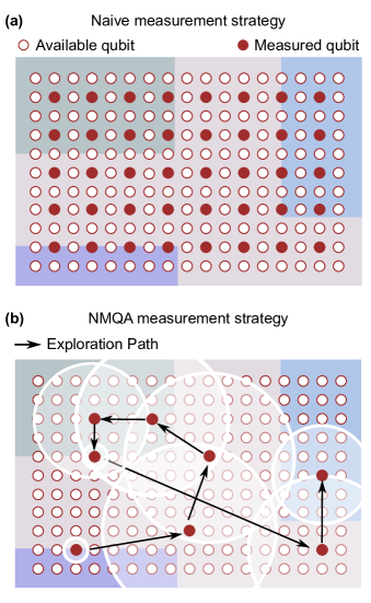
Figure 1: Difference between a naive brute force and the NMQA measurement strategy in reconstructing an inhomogenous background field. A spatial arrangement of qubits (red circles) is shown with a true unknown field with finite correlations (colored regions). (a) The naive strategy measures the field across the array using a regular grid (red filled circles). (b) The NMQA strategy iteratively chooses which qubit to measure next (black arrows) and additionally stores state estimation information in a form shared across local neighborhoods (white shaded circles), which reflects the spatial characteristics of the underlying map.

The simplest approach to the mapping problem is to undertake a brute-force, “naive” strategy in which one uniformly measures sensor-qubits across the array, depicted schematically in  Fig. 1(a). By extensively sampling qubit locations in space repeatedly, one can build a map of the underlying noise fields through the collection of large amounts of measurement information. Evidently, the naive, brute-force measurement approach is highly inefficient as it fails to recognize and exploit spatial correlations in the underlying noise field that may exist over a length-scale that exceeds the inter-qubit spacing. This is a particular concern in circumstances where qubit measurements are a costly resource e.g. in time, classical communications bandwidth, or qubit utilization when sensors are dynamically allocated.

The NMQA framework shown in Fig. 1(b) stands in stark contrast, taking inspiration from the problem of simultaneous localization and mapping in robotic control Cadena et al. (2016); Bergman (1999); Stachniss et al. (2014); Durrant-Whyte and Bailey (2006); Bailey and Durrant-Whyte (2006); Murphy (2000); Howard (2006); Thrun et al. (2005, 1998). Here the underlying spatial correlations of the noise are mapped using a learning procedure, which adaptively determines the location of the next, most-relevant measurement to be performed based on past observations. With this approach, NMQA reduces the overall resources required for spatial noise mapping by actively exploiting the spatial correlations to decide whether measurements on specific qubits provide an information gain.

We approximate the theoretical non-linear filtering problem embodied by NMQA using particle-filtering techniques. Particle filters are used to propagate and update classical probability distributions in cases where they are expected to undergo highly non-linear transformations (cf. standard particle filters Doucet et al. (2001) and their use in classical robotic mapping Beevers and Huang (2007); Grisettiyz et al. (2005); Poterjoy (2016)). In our application, the choice of a particle filter to implement core NMQA functionality accommodates the non-linear measurement model associated with the discretized outcomes given by projective qubit readout.

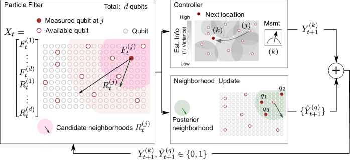
Figure 2: Schematic overview of a NMQA iteration. A particle filter estimates the map, $F_{t}$, and discovers neighborhoods (circular shaded) parameterized by $R_{t}^{(j)}$ for sharing state information about site $j$. Posterior state estimates from the particle filter are used by the controller, to choose site $k$ as the location of the next physical measurement, $Y^{(k)}_{t+1}$ based on regions of highest estimated uncertainty (middle top). Meanwhile, posterior state estimates are also used to share information at $j$ within the posterior neighborhood, $Q$ via data messages, $\hat{Y}^{(q)}_{t+1}$, between all neighbouring qubits $q\in Q$ (middle bottom) before commencing the next iteration. The input / output information loop is the outermost loop formed by a single physical measurement (in notation, $Y$) and a set of data messages (in notation, $\hat{Y}$). The arrow to site $k$ from $j$ does not relate to the transfer of any information, but rather, adaptive measurement scheduling by the controller to maximize information utility from the next physical measurement choice $k$.

In our particle filtering implementation, at every iteration $t$, the information about the true map is contained in the state vector, $X_{t}$. Here the word ‘state’ refers to all quantities being inferred statistically from data, as opposed to an actual physical quantum state. Aside from information about the true map, the state vector, $X_{t}$, additionally contains information, $R_{t}$, which approximate spatial gradients on the true map. The probability distribution of $X_{t}$ conditioned on data is called the posterior distribution and it summarizes our best knowledge of the true map and its approximate spatial gradient information given past measurement outcomes. The posterior distribution is approximately represented as a discrete collection of weighted ‘particles’. Each particle has two properties: a position and a weight. The position of the particle is effectively a hypothesis about the state $X_{t}$ i.e. a sample from the probability distribution for $X_{t}$ given observed data. The weight specifies the likelihood or the importance of the particle in the estimation procedure. All weights are initially equal at step $t=0$ and after receiving measurement data at each step, the particles are ‘re-sampled’. This means that the original set of particles at step $t$ is replaced by a set of “offspring” particles, where the probability that a parent is chosen to represent itself in the next iteration (with replacement) is directly proportional to its weight. Over many iterations, only the particles with the highest weights survive and these surviving particles form the estimate of the distribution of $X_{t}$ given data, in our algorithm. At any $t$, the estimate of $X_{t}$ can be obtained as the first moment of the posterior particle distribution, and similarly, true state uncertainty is estimated from the empirical variance of the particle distribution.

The key operating principle of NMQA is that we locally estimate the map value, $F_{t}^{(j)}$ (a qubit phase shift with value between $[0,\pi]$ radians), before globally sharing the map information at the measured qubit $j$ with neighboring qubits $q\in Q_{t}$ in the vicinity of $j$. The algorithm is responsible for determining the appropriate size of the neighborhood, $Q_{t}$, parameterized by the length-scale value, $R_{t}^{(j)}$ (left panel, Fig. 2). In practice, $Q_{t}$ eventually represents the set of qubits in a posterior neighborhood at $j$ at the end of iteration $t$, and this set shrinks or grows as inference proceeds. We are ignorant, a priori, of any knowledge of $R_{t=0}^{(j)}$ and estimates take values between $R_{min}$, approximately the inter-qubit spacing, and $R_{max}$, the size of the qubit array, in units of distance. The collection of map values and length-scales, $X_{t}^{(j)}:=\{F_{t}^{(j)},R_{t}^{(j)}\}$, at every qubit, $j=1,2,\ldots d$, is depicted as an extended state vector.

We rely on an iterative maximum likelihood procedure within each iteration of the particle filter to solve the NMQA inference problem, as the size of the state-space generally impedes analytic solutions even in classical settings Thrun et al. (2005); Thrun (2001). In each iteration, we update $F_{t}$ assuming $X_{t-1}$ is known, and subsequently update $R_{t}$ based on $F_{t}$. This structure is unique and requires two particle types; $\alpha$ particles carry information about the full state vector, $X_{t}$, while $\beta$ particles discover the optimal information-sharing neighborhood size, $R_{t}^{(j)}$, around qubit $j$. The two different types of particle sets are then used to manipulate the joint probability distribution defined over $F_{t}$ and $R_{t}$ such that we numerically implement an iterative maximum likelihood procedure. The final result of the particle filtering step in Fig. 2 is a posterior estimate of $X_{t}$ which represents our best knowledge given measurement data.

This estimate is now passed to an autonomous measurement scheduler, the NMQA controller, which attempts to maximize the information utility from each measurement. The NMQA controller adaptively selects the location $k$ for the next physical measurement by choosing the region where posterior state variance is maximally uncertain (Fig. 2, top-middle panel), and that new measurement outcome, once collected, is denoted $Y_{t+1}^{(k)}$ (a posterior state variance is typically estimated using the properties of particles inside the filter Bain and Crisan (2009)). Meanwhile, the posterior state information at step $t$ is also shared with the set $Q_{t}$ in the vicinity of qubit $j$ (Fig. 2, bottom-middle panel). The shared information within this neighborhood is denoted by the set $\{\hat{Y}_{t+1}^{(q)},q\in Q_{t+1}\}$ and serves as an effective state estimate that is taken as an input to the algorithm in a manner similar to a physical measurement. Jointly, the new actual physical measurement, $Y_{t+1}^{(k)}$, and the set of shared information $\{\hat{Y}_{t+1}^{(q)}\}$ form the inputs for the next iteration, $t+1$. Further technical information on the overall NMQA implementation is presented in Methods.

We now provide a summary of the particle-filtering implementation used here, and highlight modifications that are unique to NMQA. Under the conditions articulated above, the NMQA filtering problem requires only two specifications: a prior or initial distribution for the state vector, $X_{0}$, at $t=0$, and a likelihood function that assigns each particle with an appropriate weight based on measurement data. Assuming a uniform prior, we only need to define the global likelihood function incorporating both particle-types. We label $\alpha$-particles by the set of numbers $\{1,2,\ldots,n_{\alpha}\}$; for each $\alpha$ particle, we also associate a set of $\beta$ particles denoted $\beta^{(\alpha)}$, with $\beta$ taking values $\{1,2,\ldots,n_{\beta}\}$. Each $\alpha$ particle is weighted or scored by a so-called likelihood function. This likelihood function is written in notation as $g_{1}(\lambda_{1},Y_{t}^{(j)})$, where $\lambda_{1}$ is a parameter of the NMQA model and $Y_{t}^{(j)}$ makes explicit that only one physical measurement at one location is received per iteration. A single $\beta^{(\alpha)}$-particle inherits the state from its $\alpha$-parent, but additionally acquires a single, uniformly distributed sample for $R_{t}^{(j)}$ from the length-scale prior distribution. The $\beta$-particles are scored by a separate likelihood function, $g_{2}(\lambda_{2},Q_{t})$, where $\lambda_{2}$ is another parameter of the NMQA model. Then the total likelihood for an $(\alpha,\beta^{(\alpha)})$ pair is given by the product of the $\alpha$ and $\beta$ particle weights.

The functions $g_{1}(\lambda_{1},Y_{t}^{(j)})$ and $g_{2}(\lambda_{2},Q_{t})$ are likelihood functions used to score particles inside the NMQA particle filter, and their mathematical definitions can be found in the Supplementary Materials. These functions are derived by representing the noise affecting the physical system via probability density functions. The function $g_{1}(\lambda_{1},Y_{t}^{(j)})$ describes measurement noise on a local projective qubit measurement as a truncated or a quantized Gaussian error model to specify the form of the noise density function. The function $g_{2}(\lambda_{2},Q_{t})$ represents the probability density of “true errors” arising from choosing an incorrect set of neighbourhoods while building the map. For each candidate map, the value of the field at the center is extrapolated over the neighborhood using a Gaussian kernel. Thus, what we call “true errors” are the differences between the values of the true, spatially continuous map and the NMQA estimate, consisting of a finite set of points on a map and their associated (potentially overlapping) Gaussian neighborhoods. We assume that these errors are truncated Gaussian distributions with non-zero means and variances over many iterations.

The two free parameters, $\lambda_{1},\lambda_{2}\in[0,1]$, are used to numerically tune the performance of the NMQA particle filter. Practically, $\lambda_{1}$ controls how shared information is aggregated when estimating the value of the map locally and $\lambda_{2}$ controls how neighborhoods expand or contract in size with each iteration. Additionally, the numerically tuned values of $\lambda_{1},\lambda_{2}\in[0,1]$ provide an important test of whether or not the NMQA sharing mechanism is trivial in a given application. Non-zero values suggest that sharing information spatially actually improves performance more than just locally filtering observations for measurement noise. As $\lambda_{1},\lambda_{2}\to 1$, the set $\{\hat{Y}_{t+1}^{(q)}\}$, is treated as if they were the outcomes of real physical measurements by the algorithm. However, in the limit $\lambda_{1},\lambda_{2}\to 0$, no useful information sharing in space occurs, and NMQA effectively reduces to the naive measurement strategy.

Detailed derivations for mathematical objects and computations associated with NMQA, and an analysis of their properties using standard non-linear filtering theory, will be provided in a forthcoming technical manuscript.

III Results

Application of the NMQA algorithm using both numerical simulations and real experimental data demonstrates the capabilities of this routine for a range of spatial arrangements of $d$ qubits in 1D or 2D. Our evaluation procedure begins with the identification of a suitable metric for characterizing mapping performance and efficiency. We choose a Structural SIMilarity Index (SSIM)  Wang et al. (2004), frequently used to compare images in machine learning analysis. This metric compares the structural similarity between two images and is defined mathematically in Methods. It is found to be sensitive to improvements in the quality of images while giving robustness against e.g. large single-pixel errors that frequently plague norm-based metrics for vectorized images Chen et al. (2009); Wang and Bovik (2009). In our approach, we compare the true map and its algorithmic reconstruction by calculating the SSIM; a score of zero corresponds to ideal performance, and implies that the true map and its reconstruction are identical.

We start with a challenging simulated example, in which $d=25$ qubits are arranged in a 2D grid. The true field is partitioned into square regions with relatively low and high values (Fig. 3(a), left inset) to provide a clear structure for the mapping procedure to identify. In this case, the discontinuous change of the field values in space means that NMQA will not be able to define a low-error candidate neighborhood for any qubits on the boundary. Both NMQA and naive are executed over a maximum of $T$ iterations such that $t\in[1,T]$. For simplicity, in most cases, we pick values of $T\geq d$ as multiples of the number of qubits, $d$, such that every qubit is measured the same integer number of times in the naive approach which we use as baseline in our comparison. If $T<d$, the naive approach uniformly randomly samples qubit locations. Both NMQA and the naive approach terminate when $t=T$, and a single-run SSIM score is calculated using the estimated map for each algorithm in comparison with the known underlying “true” noise map. The average value of the score over 50 trials is reported as Avg. SSIM.

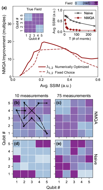
Figure 3: (a) Upper left inset: 2D array of 25 qubits with ‘square’ field shown as a colorscale. Upper right inset: Avg. SSIM score vs total measurement budget $T$ for NMQA and naive algorithms averaged over 50 trials. Main panel: ratio of naive to NMQA measurements vs. Avg. SSIM score for tuned $\lambda_{1},\lambda_{2}$ (solid line) at each $T$; fixed choice $\lambda_{1}=0.89,\lambda_{2}=0.97$ (dashed line) tuned for $T=20$. The numerical inversion of raw data in the upper right inset introduces artifacts and is unstable for small Avg. SSIM scores. (b)-(e) Columns show single-run maps using a total number of $T=10$ or $T=75$ measurements plotted for the NMQA (b, c) and naive approach (d, e), with a representative control path shown in (b). The numerically tuned parameters are $(\lambda_{1},\lambda_{2})=(0.89,0.97)$ and $(0.93,0.68)$ for (b),(c) respectively. The single map SSIM values are: (b) 0.37; (c) 0.09; (d) 0.8; (e) 0.47. Other parameters: $d=25$; $T=5,10,15,20,25,50,75,100,125,250$; $\Sigma_{v}=10^{-4}$, $\Sigma_{F}=10^{-6}$; true low and high field values of $0.25\pi$ and $0.75\pi$ radians respectively.

The Avg. SSIM score as a function of $T$ is shown in the upper right inset of Fig. 3(a). For any choice of $T$, NMQA reconstructs the true field with a lower SSIM than the naive approach, indicating better performance. The SSIM score also drops rapidly with $T$ when using NMQA, compared with a more gradual decline in the naive case. Increasing $T\gg d$ leads to an improvement in the performance of both algorithms but also a convergence of the scores as every qubit is likely to be measured multiple times for the largest values considered here. Representative maps for $T=10$ and $T=75$ measurements under both the naive and NMQA mapping approaches are shown in Fig. 3(b-e), along with a representative adaptive measurement sequence employed in NMQA in panel (b). In both cases, NMQA provides estimates of the map which are closer to the true field values, whereas naive maps are dominated by estimates at the extreme ends of the range, which is characteristic for simple reconstructions using sparse measurements. It is instructive to represent these data in a form that shows the effective performance enhancement of the NMQA mapping procedure relative to the naive approach; the main panel in Fig. 3(a) reports the improvement in the reduction of the number of measurements required to reach a desired Avg. SSIM value. The shape of the performance improvement curve is linked to the total amount of information provided to both algorithms. At high Avg. SSIM scores on the far-right of the figure, both naive and NMQA algorithms receive very few measurements and map-reconstructions are dominated by errors. Near the origin, an extremely large number of measurements are required to achieve low Avg. SSIM scores and the ratio of measurements between naive and NMQA tends to unity, corresponding to the convergence mentioned above. In the intermediate regime, a broad peak indicates that NMQA outperforms brute force measurement by up to $18\times$ in reducing total number of qubit measurements over a range of moderate-to-low Avg. SSIM scores for map reconstruction error. Similar performance is achieved for a range of other qubit-array geometries and characteristics of the underlying field (Supplementary Materials).

All of our results rely on appropriate tuning of the NMQA particle filter via its parameters $\lambda_{1}$ and $\lambda_{2}$. Numerical tuning of these parameters is conducted for each $T$ and this data is represented as solid curves in Fig. 3(a). We also demonstrate that using fixed values for these parameters only marginally degrades performance, as indicated by the dashed line in Fig. 3(a).

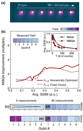
Figure 4: (a) Image of six trapped ${}^{171}\mathrm{Yb}^{+}$ ions in the fluorescing $|1\rangle$ state averaged over multiple exposures of 750 $\upmu$s. (b) Upper left inset: Color scale indicating a phase shift induced by a magnetic field gradient across 1D array of 6 qubits. Upper right inset: Avg. SSIM score vs total measurement budget $T$ for NMQA and naive algorithms averaged over 50 trials. Main panel: ratio of naive to NMQA measurements vs. Avg. SSIM score for tuned $\lambda_{1},\lambda_{2}$ (solid line) at each $T$; fixed choice $(\lambda_{1},\lambda_{2})=(0.95,0.99)$ tuned for $T=24$. The numerical inversion of raw data in the upper right inset introduces artifacts and is unstable for small SSIM scores. (c)-(f) Columns show single-run maps using a total number of $T=6$ or $T=96$ measurements plotted for the NMQA (c, d) and naive (e, f), with a representative control path shown in (c). The numerically tuned parameters are $(\lambda_{1},\lambda_{2})=(0.97,0.94)$ for (c) and $(0.97,0.95)$ for (d). Single map SSIM values are (c) 0.99; (d) 0.35; (e) 0.77; (f) 0.50. Other parameters: $d=6$; $T=1,2,3,4,6,12,18,24,30,60,72,96,120,246$; $\Sigma_{v}=10^{-4}$, $\Sigma_{F}=10^{-6}$; true low and high field values of $0.25\pi$ and $0.75\pi$ radians respectively.

We now apply the NMQA mapping algorithm to real experimental measurements on qubit arrays. In Fig. 4, we analyze Ramsey experiments conducted on an array of ${}^{171}\text{Yb}^{+}$ ions confined in a linear Paul trap, with trap frequencies $\omega_{x,y,z}/2\pi\approx(1.6,1.5,0.5)~{}\text{MHz}$. Qubits are encoded in the ${}^{2}\mathrm{S}_{1/2}$ ground-state manifold where we associate the atomic hyperfine states $|F=0,m_{F}=0\rangle$ and $|F=1,m_{F}=0\rangle$ with the qubit states $|0\rangle$ and $|1\rangle$, respectively. State initialization to $|0\rangle$ via optical pumping and state detection are performed using a laser resonant with the ${}^{2}\mathrm{S}_{1/2}-{{}^{2}\mathrm{P}_{1/2}}$ transition near 369.5 nm. Laser-induced fluorescence (corresponding to projections into state $|1\rangle$) is recorded using a spatially resolving EMCCD camera yielding simultaneous readout of all ions. In this experiment, qubit manipulation is carried out using microwave radiation at 12.6 GHz delivered via an in-vacuum antenna to all qubits globally.

The trapped ions experience an uncontrolled (“intrinsic”), linear magnetic field gradient which produces spatially inhomogeneous qubit frequencies over the trap volume. When manipulated using a global microwave control field, this results in a differential phase accumulation between qubits. The magnitude of the gradient is illustrated in Fig. 4(a), superimposed on an image of six ions in the bright state $|1\rangle$. We aim to probe this field gradient through the resulting qubit detuning and associated differential phase accumulation throughout each measurement repetition.

A preliminary Ramsey experiment, in which the interrogation time is varied and fringes observed, confirms that at an interrogation time of $40$ms accumulated relative phase in a Ramsey measurement is $<\pi$ radians. A total of $25,500$ Ramsey measurements with a wait time of $40$ ms are performed on all six ions in parallel. For each repetition, a standard machine-learning image classification algorithm assigns a ‘0’ (dark) or ‘1’ (bright) to each ion based on a previously recorded set of training data. From averaging over repetitions, we construct a map of the accumulated phase (and hence the local magnetic field inducing this phase) on each qubit, shown schematically in the right inset of Fig. 4(b). We consider the field extracted from this standard averaging procedure over all repetitions of the Ramsey experiment, at each ion location, as the “true” field against which mapping estimates are compared using the SSIM score as introduced above.

We employ the full set of $6\times 25,500$ measurements as a data-bank on which to evaluate and benchmark both algorithms. At each iteration, the algorithm determines a measurement location in the array and then randomly draws a single, discretized measurement outcome (0 or 1) for that ion from the data-bank. The rest of the algorithmic implementation proceeds as before. Accordingly, we expect that the naive approach must smoothly approach a SSIM score of zero as $T$ increases (Fig. 4(b), left inset). In these experiments, we experience a large measurement error arising from the necessary detection time of 750 $\upmu$s associated with the relatively low quantum efficiency and effective operating speed of the EMCCD camera. Performing spatially resolved measurement across the qubit array introduces a large measurement error due to the low quantum efficiency of the EMCCD camera. Compensating this via extension of the measurement period leads to an asymmetric bias due to state decays that occur during the measurement process in $\approx 1.5$ ms ($|1\rangle\rightarrow|0\rangle$) and $\approx 30$ ms ($|0\rangle\rightarrow|1\rangle$) under the laser power and quantization magnetic field strength used in our experiment. In our implementation, neither NMQA nor the brute-force algorithm was modified to account for this asymmetric bias in the detection procedure, although in principle the image classification algorithm employed to determine qubit states from fluorescence detection can be expanded to account for this. Therefore, both NMQA and the naive approach are affected by the same detection errors. Despite this complication, we again find that NMQA outperforms the naive mapping algorithm by a factor of $2-3$ in the number of required measurements (Fig. 4(b)), with expected behavior at the extremal values of Avg. SSIM.

IV Conclusion

In this work we presented NMQA - a framework for autonomous learning where we reconstruct an unknown spatial noise field by efficiently scheduling measurements on multi-qubit devices. We developed a novel, iterative, maximum-likelihood procedure implemented via a two-layer particle filter to share state-estimation information between qubits within small spatial neighborhoods, via a mapping of the underlying spatial correlations of the noise field. An autonomous controller schedules future measurements in order to reduce the estimated uncertainty of the map reconstruction. Numerical simulations and calculations run on real experimental data demonstrated that NMQA outperforms a naive mapping procedure by reducing the required number of measurements up to $3\times$ in achieving a target map similarity score on a 1D array of trapped ytterbium ions (up to $18\times$ in 2D using simulated data).

Beyond these example demonstrations, the key numerical evidence for the correctness of NMQA’s functionality came from the observation that the tuned values of $\lambda_{1},\lambda_{2}\gg 0$ for all results reported here. Since numerically tuned values for these parameters were found to be non-zero, we conclude information sharing in NMQA is non-trivial and the algorithm departs substantially from a brute-force measurement strategy. This contributes to the demonstrated improvements in Avg. SSIM scores when using NMQA in Figs. 3 and 4.

Overall, achieving suitable autonomous learning through NMQA requires that the $(\lambda_{1},\lambda_{2})$ parameters are appropriately tuned using measurement data-sets as part of a training procedure. To select $(\lambda_{1},\lambda_{2})$, we chose a $(\lambda_{1},\lambda_{2})$ pair with the lowest expected error. Such an error calculation requires apriori information about the measured (or true) field, with the expected value computed over many runs. Numerical analysis shows that tuned $\lambda_{1},\lambda_{2}\in[0.5,1]$ (top right quadrant of the unit square) and this observation holds for a range of different noise fields with regularly spaced 1D or 2D configurations. These numerical observations suggest that theoretical approaches to deducing ‘optimal’ regions for $(\lambda_{1},\lambda_{2})$ may be possible. Meanwhile, in a specific application, a practitioner may only have access to the real-time rate of change of state estimates and residuals, i.e. a particle filter generates a predicted measurement at location $j$ which can be compared to next the actual measurement received at $j$. Monitoring the real-time rate of change of state estimates and/or residuals in a single run can be used to develop effective stopping criteria to set $(\lambda_{1},\lambda_{2})$ with minimal apriori knowledge of the physical system. These extensions to the operability of NMQA are active research areas.

The framework we have introduced is flexible and can accommodate temporal variations in the system such as drifts in the map and changes in the availability of sensor qubits. We are also excited to explore how exploitation of hardware platforms in which qubit locations are not rigidly fixed during fabrication, such as with trapped-ions, may allow sub-lattice spatial resolution by dynamically translating individual qubits during the mapping procedure. Our work is part of an exciting new area of future study exploring the intersection between hardware architectures and control solutions Ball et al. (2016) in NISQ-era quantum computers, and may also have bearing on distributed networks of quantum sensors.

Methods

We summarize the structure of the NMQA algorithm in Algorithm 1 using a pseudocode representation.

The first part of the algorithm consists of an initialization procedure which ensures all particles are sampled from the prior for extended state vector at $t=0$, giving $X_{0}$. All particles are equally weighted before measurement data is received.

Algorithm 1 NMQA

procedure NMQA($d$ qubit locations, $\lambda_{1},\lambda_{2}$)

     if $t=0$ then

         procedure Initialize($X_{0}$)

              for $\alpha\in\{1,2,\ldots,n_{\alpha}\}$ do

                  Initially sample $x_{0}^{(\alpha)}\sim\pi_{0}$

                  Initially compute $W_{0}^{(\alpha)}=\frac{1}{n_{\alpha}}$

              end for

         end procedure

     end if

     while $1\leq t<T$ do

         if Controller then

              $j_{t},Y_{t}^{(j_{t})}\leftarrow$ Controller($X_{t-1}$) $\triangleright$ Qubit $j$, at $t$

         end if

         for $\alpha\in\{1,2,\ldots,n_{\alpha}\}$ do

              $\{x_{t}^{(\alpha)}\}\leftarrow$ PropagateStates($\{x_{t-1}^{(\alpha)}\}$ )

              Update $F_{t}^{(\cdot),(\alpha)}$ via $\{Y_{t}^{(j_{t})},\{\hat{Y}_{t}^{(q_{t})}\},\lambda_{1}\}$

              $\{\{x_{t},W_{t}\}^{(\alpha,\beta_{\alpha})}\}\leftarrow$ ComputeWeights($\{x_{t}^{(\alpha)}\}$)

              $\{x_{t}^{(\alpha,\beta_{\alpha})},\frac{1}{n_{\alpha}n_{\beta}}\}\leftarrow$ Resample($\{\{x_{t},W_{t}\}^{(\alpha,\beta_{\alpha})}\}$)

              Update $R_{t}^{(j_{t}),(\alpha)}$

              $\{\{x_{t},W_{t}\}^{(\alpha)}\}\leftarrow$ Collapse$\beta$($\{x_{t}^{(\alpha,\beta_{\alpha})},\frac{1}{n_{\alpha}n_{\beta}}\}$)

              $\{x_{t}^{(\alpha)},\frac{1}{n_{\alpha}}\}\leftarrow$ Resample($\{\{x_{t},W_{t}\}^{(\alpha)}\}$)

         end for

         $\{\hat{Y}_{t+1}^{(q)}\}_{q\in Q_{t+1}}\leftarrow$ Generate$\hat{Y}$(Posterior $X_{t}$)

     end while

end procedure

function ComputeWeights($\{x_{t}^{\alpha}\}$)

     for $\alpha\in\{1,2,\ldots,n_{\alpha}\}$ do

         Compute $\tilde{W}_{t}^{(\alpha)}=g_{1}(\lambda_{1},Y_{t}^{(j)})$

         $\{x_{t}^{(\alpha,\beta_{\alpha})}\}\leftarrow$ Generate $\beta$-layer

         for $\beta_{\alpha}\in\{1,2,\ldots,n_{\beta}\}$ do

              Compute $\tilde{W}_{t}^{(\beta_{\alpha}|\alpha)}=g_{2}(\lambda_{2},Q_{t})$

         end for

         Normalize $\tilde{W}_{t}^{(\beta_{\alpha}|\alpha)}$

     end for

     Normalize $\tilde{W}_{t}^{(\alpha)}$

     Compute $W_{t}^{(\alpha,\beta_{\alpha})}=\tilde{W}_{t}^{(\beta_{\alpha}|\alpha)}\tilde{W}_{t}^{(\alpha)}\quad\forall\{\alpha,\{\beta_{\alpha}\}\}$

     Return $n_{\alpha}n_{\beta}$ particles and weights $\{\{x_{t},W_{t}\}^{(\alpha,\beta_{\alpha})}\}$

end function

For $t>0$, the function PropagateStates represents the transition probability distribution for Markov $X_{t}$ i.e. it represents identity dynamics and is a placeholder for future extensions to model dynamical $F_{t}$. In each $t$, a single physical measurement is received. This triggers a set of update rules for $F_{t}$ and $R_{t}$. We note that the state variables, $F_{t}$ and $R_{t}$, are updated in a specific order within each time-step $t$. The order of these computations correspond to the iterative maximum likelihood approximation for the NMQA framework. The form of the update rules reflect NMQA’s unique state vector and NMQA’s information sharing procedures. Map and neighborhood information is carried via different particle types, and information sharing is implemented via particle updates and re-sampling steps. For each type of particle, the weights are computed according to NMQA likelihood functions $g_{1}(\lambda_{1},Y_{t}^{(j)})$ and $g_{2}(\lambda_{2},Q_{t})$.

Despite atypical computational steps and unique likelihood functions, the total number of particles is constant at the beginning and end of each time-step $t$ and the particle branching mechanism for NMQA remains a multi-nomial branching process. These multi-nomial branching processes are characteristic of standard particle filtering techniques Bain and Crisan (2009).

IV.1 Structural Similarity Metric Definition

For all analysis, we use a risk metric called the Structural Similarity Index (SSIM) Wang et al. (2004). This metric is used to conduct optimization of NMQA parameters and assess performance relative to the naive measurement strategy. For two vectorized images $x$ and $y$, the metric is defined as:

$$s(x,y) =\frac{(2\mu_{x}\mu_{y}+C_{1})(2\sigma_{xy}+C_{2})}{(\mu_{x}^{2}+\mu_{y}^{2}+C_{1})(\sigma_{x}^{2}+\sigma_{y}^{2}+C_{2})}$$ (1)

$$\text{SSIM}(x,y) :=|1-s(x,y)|$$ (2)

In the formula above, $\mu_{i},\sigma_{i}^{2},i=x,y$ represent the sample estimates of the means and variances of the respective vectorized images, and $\sigma_{xy}$ captures correlation between images. The term $s(x,y)$ is the key metric developed in Wang et al. (2004) and it includes arbitrary constants $C_{1}=C_{2}=0.01$ which stabilize the metric for images with means or variances close to zero. The ideal score given by $s(x,y)$ is unity, and corresponds uniquely to the case $x=y$. We report the absolute value of the deviations from the ideal score of unity, where the direction of the deviation is ignored as given by $\text{SSIM}(x,y)$. For our application, this $\text{SSIM}(x,y)$ metric lies between $[0,1]$ (negative values of $s(x,y)$ are not seen in our numerical demonstrations). We report the average of $\text{SSIM}(x,y)$ values over 50 trials as Avg. SSIM.

Data Availability

All simulated and experimental data to reproduce all figures can be accessed via links in the Supplementary Materials without restrictions.

Code Availability

Minimally reproducing equations for NMQA and links to the code-base are provided in the Supplementary Materials without restrictions.

Author Contributions

The NMQA theoretical framework and numerical implementations were devised by R. Gupta based on research directions set by M.J. Biercuk. R. Gupta and M.J. Biercuk co-wrote the paper. A. Milne, C. Edmunds and C. Hempel led all experimental efforts and contributed to the paper draft.

Competing Interests

The authors declare that there are no competing interests.

V Materials and Correspondence

Correspondence to R. Gupta.

References

- Preskill (2018) John Preskill, “Quantum Computing in the NISQ era and beyond,” Quantum 2, 79 (2018).
- Yao et al. (2012) Norman Y Yao, Liang Jiang, Alexey V Gorshkov, Peter C Maurer, Geza Giedke, J Ignacio Cirac, and Mikhail D Lukin, “Scalable architecture for a room temperature solid-state quantum information processor,” Nature communications 3, 800 (2012).
- Monroe et al. (2014) C Monroe, R Raussendorf, A Ruthven, KR Brown, P Maunz, L-M Duan, and J Kim, “Large-scale modular quantum-computer architecture with atomic memory and photonic interconnects,” Physical Review A 89, 022317 (2014).
- Veldhorst et al. (2017) M Veldhorst, HGJ Eenink, CH Yang, and AS Dzurak, “Silicon CMOS architecture for a spin-based quantum computer,” Nature communications 8, 1766 (2017).
- Jones et al. (2012) N Cody Jones, Rodney Van Meter, Austin G Fowler, Peter L McMahon, Jungsang Kim, Thaddeus D Ladd, and Yoshihisa Yamamoto, “Layered architecture for quantum computing,” Physical Review X 2, 031007 (2012).
- Kielpinski et al. (2002) David Kielpinski, Chris Monroe, and David J Wineland, “Architecture for a large-scale ion-trap quantum computer,” Nature 417, 709 (2002).
- Franke et al. (2019) David P Franke, James S Clarke, Lieven MK Vandersypen, and Menno Veldhorst, “Rent’s rule and extensibility in quantum computing,” Microprocessors and Microsystems (2019).
- Ball et al. (2016) Harrison Ball, Trung Nguyen, Philip H. W. Leong, and Michael J. Biercuk, “Functional basis for efficient physical layer classical control in quantum processors,” Phys. Rev. Applied 6, 064009 (2016).
- Brown et al. (2004) Kenneth R. Brown, Aram W. Harrow, and Isaac L. Chuang, “Arbitrarily accurate composite pulse sequences,” Phys. Rev. A 70, 052318 (2004).
- Merrill and Brown (2014) J. True Merrill and Kenneth R. Brown, “Progress in compensating pulse sequences for quantum computation,” in Quantum Information and Computation for Chemistry (John Wiley & Sons, Inc., 2014) pp. 241–294.
- Khodjasteh and Viola (2009) K. Khodjasteh and L. Viola, “Dynamically error-corrected gates for universal quantum computation,” Phys. Rev. Lett. 102, 080501 (2009).
- Soare et al. (2014) A. Soare, H. Ball, D. Hayes, J. Sastrawan, M. C. Jarratt, J. J. McLoughlin, X. Zhen, T. J. Green, and M. J. Biercuk, “Experimental noise filtering by quantum control,” Nat. Phys. 10 (2014).
- Paz-Silva and Viola (2014) Gerardo A. Paz-Silva and Lorenza Viola, “General transfer-function approach to noise filtering in open-loop quantum control,” Phys. Rev. Lett. 113, 250501 (2014).
- Kabytayev et al. (2014) Chingiz Kabytayev, Todd J. Green, Kaveh Khodjasteh, Michael J. Biercuk, Lorenza Viola, and Kenneth R. Brown, “Robustness of composite pulses to time-dependent control noise,” Phys. Rev. A 90, 012316 (2014).
- Venturelli et al. (2018a) Davide Venturelli, Minh Do, Eleanor Rieffel, and Jeremy Frank, “Compiling quantum circuits to realistic hardware architectures using temporal planners,” Quantum Science and Technology 3, 025004 (2018a).
- Murali et al. (2019) Prakash Murali, Jonathan M Baker, Ali Javadi Abhari, Frederic T Chong, and Margaret Martonosi, “Noise-adaptive compiler mappings for noisy intermediate-scale quantum computers,” arXiv preprint arXiv:1901.11054 (2019).
- Shi et al. (2019) Yunong Shi, Nelson Leung, Pranav Gokhale, Zane Rossi, David I Schuster, Henry Hoffman, and Fred T Chong, “Optimized compilation of aggregated instructions for realistic quantum computers,” arXiv preprint arXiv:1902.01474 (2019).
- Venturelli et al. (2018b) Davide Venturelli, Minh Do, Kyle Booth, Eleanor Rieffel, Jeremy Frank, and Christopher Beck, “Optimization and planning approaches for low-level hardware compilation of quantum circuits,” in APS Meeting Abstracts (2018).
- Tannu and Qureshi (2018) Swamit S Tannu and Moinuddin K Qureshi, “A case for variability-aware policies for NISQ-era quantum computers,” arXiv preprint arXiv:1805.10224 (2018).
- Gelb (1974) Arthur Gelb, Applied optimal estimation (MIT press, 1974).
- Landau et al. (2011) Ioan Doré Landau, Rogelio Lozano, Mohammed M’Saad, and Alireza Karimi, Adaptive control: algorithms, analysis and applications (Springer Science & Business Media, 2011).
- Mavadia et al. (2017) Sandeep Mavadia, Virginia Frey, Jarrah Sastrawan, Stephen Dona, and Michael J. Biercuk, “Prediction and real-time compensation of qubit decoherence via machine learning,” Nature Communications 8, 14106 EP – (2017).
- Gupta and Biercuk (2018) Riddhi Swaroop Gupta and Michael J Biercuk, “Machine learning for predictive estimation of qubit dynamics subject to dephasing,” Physical Review Applied 9, 064042 (2018).
- Cooper et al. (2014) A. Cooper, E. Magesan, H. N. Yum, and P. Cappellaro, “Time-resolved magnetic sensing with electronic spins in diamond,” Nature Communications 5, 3141 EP – (2014).
- Brown et al. (2016) Kenneth R Brown, Jungsang Kim, and Christopher Monroe, “Co-designing a scalable quantum computer with trapped atomic ions,” NPJ Quantum Information 2, 16034 EP – (2016).
- Hirose and Cappellaro (2016) Masashi Hirose and Paola Cappellaro, “Coherent feedback control of a single qubit in diamond,” Nature 532, 77 EP – (2016).
- Postler et al. (2018) Lukas Postler, Ángel Rivas, Philipp Schindler, Alexander Erhard, Roman Stricker, Daniel Nigg, Thomas Monz, Rainer Blatt, and Markus Müller, “Experimental quantification of spatial correlations in quantum dynamics,” arXiv preprint arXiv:1806.08088 (2018).
- Cadena et al. (2016) Cesar Cadena, Luca Carlone, Henry Carrillo, Yasir Latif, Davide Scaramuzza, José Neira, Ian Reid, and John J Leonard, “Past, present, and future of simultaneous localization and mapping: Toward the robust-perception age,” IEEE Transactions on robotics 32, 1309–1332 (2016).
- Bergman (1999) Niclas Bergman, “Recursive bayesian estimation,” Department of Electrical Engineering, Linköping University, Linköping Studies in Science and Technology. Doctoral dissertation 579, 11 (1999).
- Stachniss et al. (2014) Cyrill Stachniss, Wolfram Burgard, et al., “Particle filters for robot navigation,” Foundations and Trends® in Robotics 3, 211–282 (2014).
- Durrant-Whyte and Bailey (2006) Hugh Durrant-Whyte and Tim Bailey, “Simultaneous localization and mapping: Part I, robotics & automation magazine,” IEEE 13, 99–110 (2006).
- Bailey and Durrant-Whyte (2006) Tim Bailey and Hugh Durrant-Whyte, “Simultaneous localization and mapping (SLAM): Part II,” IEEE Robotics & Automation Magazine 13, 108–117 (2006).
- Murphy (2000) Kevin P Murphy, “Bayesian map learning in dynamic environments,” in Advances in Neural Information Processing Systems (2000) pp. 1015–1021.
- Howard (2006) Andrew Howard, “Multi-robot simultaneous localization and mapping using particle filters,” The International Journal of Robotics Research 25, 1243–1256 (2006).
- Thrun et al. (2005) Sebastian Thrun, Wolfram Burgard, and Dieter Fox, Probabilistic robotics (MIT press, 2005).
- Thrun et al. (1998) Sebastian Thrun, Wolfram Burgard, and Dieter Fox, “A probabilistic approach to concurrent mapping and localization for mobile robots,” Autonomous Robots 5, 253–271 (1998).
- Doucet et al. (2001) Arnaud Doucet, Nando De Freitas, and Neil Gordon, Sequential Monte Carlo methods in practice (Springer, 2001) pp. 3–14.
- Beevers and Huang (2007) Kristopher R Beevers and Wesley H Huang, “Fixed-lag sampling strategies for particle filtering SLAM,” in Proceedings 2007 IEEE International Conference on Robotics and Automation (IEEE, 2007) pp. 2433–2438.
- Grisettiyz et al. (2005) Giorgio Grisettiyz, Cyrill Stachniss, and Wolfram Burgard, “Improving grid-based slam with Rao-Blackwellized particle filters by adaptive proposals and selective resampling,” in Proceedings of the 2005 IEEE International Conference on Robotics and Automation (IEEE, 2005) pp. 2432–2437.
- Poterjoy (2016) Jonathan Poterjoy, “A localized particle filter for high-dimensional nonlinear systems,” Monthly Weather Review 144, 59–76 (2016).
- Thrun (2001) Sebastian Thrun, “A probabilistic on-line mapping algorithm for teams of mobile robots,” The International Journal of Robotics Research 20, 335–363 (2001).
- Bain and Crisan (2009) Alan Bain and Dan Crisan, Fundamentals of Stochastic Filtering, Stochastic Modelling and Applied Probability (Springer, 2009).
- Wang et al. (2004) Zhou Wang, Alan C Bovik, Hamid R Sheikh, and Eero P Simoncelli, “Image quality assessment: from error visibility to structural similarity,” IEEE transactions on image processing 13, 600–612 (2004).
- Chen et al. (2009) Yihua Chen, Eric K Garcia, Maya R Gupta, Ali Rahimi, and Luca Cazzanti, “Similarity-based classification: Concepts and algorithms,” Journal of Machine Learning Research 10, 747–776 (2009).
- Wang and Bovik (2009) Zhou Wang and Alan C Bovik, “Mean squared error: Love it or leave it? a new look at signal fidelity measures,” IEEE signal processing magazine 26, 98–117 (2009).