The surprisingly low carbon mass in the debris disk around HD 32297

Abstract

Gas has been detected in a number of debris disks. It is likely secondary, i.e. produced by colliding solids. Here, we report ALMA Band 8 observations of neutral carbon in the CO-rich debris disk around the 15–30 Myr old A-type star HD 32297. We find that C⁰ is located in a ring at $\sim$110 au with a FWHM of $\sim$80 au, and has a mass of $(3.5\pm 0.2)\times 10^{-3}$ M_⊕. Naively, such a surprisingly small mass can be accumulated from CO photo-dissociation in a time as short as $\sim$10⁴ yr. We develop a simple model for gas production and destruction in this system, properly accounting for CO self-shielding and shielding by neutral carbon, and introducing a removal mechanism for carbon gas. We find that the most likely scenario to explain both C⁰ and CO observations, is one where the carbon gas is rapidly removed on a timescale of order a thousand years and the system maintains a very high CO production rate of $\sim$15 M_⊕ Myr^-1, much higher than the rate of dust grind-down. We propose a possible scenario to meet these peculiar conditions: the capture of carbon onto dust grains, followed by rapid CO re-formation and re-release. In steady state, CO would continuously be recycled, producing a CO-rich gas ring that shows no appreciable spreading over time. This picture might be extended to explain other gas-rich debris disks.

1 Introduction

A considerable fraction of main-sequence stars are surrounded by dusty disks known as debris disks (e.g. Hughes et al., 2018). They are analogous to the asteroid belt and the Kuiper belt in the solar system, and are often interpreted as leftover products from the planet formation era. The observed dust is secondary, i.e. produced from the collisional destruction of larger (asteroidal or cometary) bodies. Observations of debris disks can constrain the composition of these bodies as well as the evolution and dynamics of extrasolar systems.

A sub-sample of debris disks, mainly surrounding young A-type stars, are observed to contain gas besides the dust. The Atacama Large Millimeter/submillimeter Array (ALMA) has been instrumental in increasing the sample of gaseous debris disks by providing sensitive observations of CO emission (e.g. Kóspál et al., 2013; Lieman-Sifry et al., 2016; Moór et al., 2017). Today, about 20 gaseous debris disks are known. The observed CO masses show a large spread. In some systems, the CO column density is so low that CO is not self-shielded against photodissociation by the interstellar radiation field (ISRF) (e.g. Marino et al., 2016; Matrà et al., 2017a, 2019). As a consequence, CO is photodissociated on a short timescale ($\sim$120 yr, Visser et al., 2009) and is therefore secondary, produced from the destruction of icy, cometary bodies (e.g. Kral et al., 2017). On the other hand, a few disks contain CO masses comparable to protoplanetary disks (e.g. Kóspál et al., 2013; Moór et al., 2017). Such high CO masses have been difficult to explain in a secondary scenario. Thus, it was suggested that these are ’hybrid’ disks, i.e. disks where secondary dust and primordial (i.e. leftover from the protoplanetary phase) gas co-exist (Kóspál et al., 2013; Moór et al., 2017; Péricaud et al., 2017). However, Kral et al. (2019); Marino et al. (2020) recently suggested that even these disks can be explained by secondary gas production if shielding of CO by neutral carbon is taken into account. Carbon is continuously produced from CO photodissociation. Eventually, the carbon column density can be high enough to attenuate dissociation of CO, allowing a large CO mass to build up.

This process might be at work in the debris disk around HD 32297. Located at a distance of $132.3\pm 1.0$ pc (Bailer-Jones et al., 2018), its spectral type has been described as A5–A7 (Fitzgerald et al., 2007; Donaldson et al., 2013; Rodigas et al., 2014) and its age has been estimated to be $\gtrsim 15$ Myr (Rodigas et al., 2014) and $<30$ Myr (Kalas, 2005). The dust component of the disk has been studied in considerable detail, both in scattered light (e.g. Boccaletti et al., 2012; Currie et al., 2012; Asensio-Torres et al., 2016) and thermal emission (e.g. Maness et al., 2008; Donaldson et al., 2013; MacGregor et al., 2018). Gas has been observed in the form of CO (Greaves et al., 2016; MacGregor et al., 2018), C II (Donaldson et al., 2013) and Na I (Redfield, 2007). Since the ¹²CO emission is optically thick, Moór et al. (2019) recently used observations of the ¹³CO and C¹⁸O isotopologues to constrain the total CO mass. They argue that the large CO mass can indeed be explained by secondary CO production combined with C shielding.

As carbon is the direct descendent of CO, and because of the pivotal role it plays in shielding CO, observations of carbon are an important tool to improve our understanding of gaseous debris disks. In this paper, we present ALMA observations of neutral carbon emission towards HD 32297. We attempt to explain the observations with a secondary gas production scenario. Our paper is structured as follows: in section 2, we describe our observations. In section 3, we present the data analysis and determine the spatial distribution and mass of the neutral carbon. In section 4, we present a model of the gas production and destruction. We discuss our results in section 5 and summarize in section 6.

2 Observations and data reduction

The HD 32297 disk was observed in a single pointing with ALMA Band 8 receivers on May 22, 2018, during ALMA Cycle 5 (project ID 2017.1.00201.S, PI: Cataldi). An array of 47 antennas arranged in a compact configuration was employed, with baselines ranging from 15 to 314 m. The total integration time was 45 min (with 18 min on HD 32297) and the median precipitable water vapor (pwv) was 0.6 mm.

The spectral setup consisted of three spectral windows centered at 480, 482 and 494 GHz, each with a bandwidth of 2 GHz and 128 channels to observe the dust continuum. The fourth spectral window was covering the C I ³P₁–³P₀ line at 492.16 GHz, with 1920 channels, a channel spacing of 488 kHz (0.30 km s^-1) and an effective spectral resolution of 0.34 km s^-1 (spectral averaging factor $N=2$).

The data were calibrated by the ALMA Science Pipeline within the Common Astronomy Software Applications package (CASA) 5.1.1 (McMullin et al., 2007). J0522-3627 (bandpass, flux) and J0505+0459 (phase) were observed as calibration sources.

For further processing of the calibrated visibilities, we used CASA 5.3.0. We used the task uvcontsub to subtract the continuum emission from the spectral window covering the C I line (the line was masked for the continuum fit). We produced an image cube by employing the CLEAN algorithm with the task tclean and natural weighting. The synthesized beam is $0.72\arcsec\times 0.65\arcsec$ (96 au $\times$ 86 au) with a position angle of $67\arcdeg$. The achieved noise level (measured by taking the standard deviation of a sample of data points in a region of the cube without line emission) is $1.7\times 10^{-17}$ W m^-2 Hz^-1 sr^-1 (21 mJy beam^-1). Figure 1 (left) shows the moment 0 map of the C I line, produced by integrating the data cube over the (barycentric) velocities of 15.5–25.5 km s^-1.

We also produced a continuum map (Fig. 1, right) by imaging all spectral windows combined (with the C I line masked) using the tclean task with natural weighting. The synthesized beam is $0.73\arcsec\times 0.66\arcsec$ (97 au $\times$ 88 au) with a position angle of $66\arcdeg$. The noise level (measured as above) is $2.0\times 10^{-19}$ W m^-2 Hz^-1 sr^-1 (0.25 mJy beam^-1).

The primary beam at 492 GHz has a full width at half maximum (FWHM) of $\sim$12″. This is significantly larger than the extent of the disk, so we do not apply a primary beam correction. Given our shortest baseline, the maximum recoverable scale of our observations is $\sim$5″, i.e. larger than the disk’s extent. Thus, no significant amount of flux should have been filtered out by the interferometer.

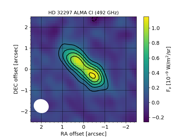
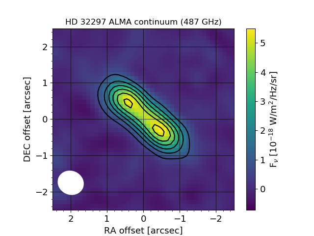
Figure 1: Left panel: Moment 0 map of the C I 492 GHz emission observed towards HD 32297. The stellar position is at $(0,0)$. Contours are drawn at intervals of 3$\sigma$, with $\sigma=7.3\times 10^{-11}$ W m^-2 sr^-1. Right panel: ALMA Band 8 continuum image at 487 GHz (616 $\mu$m). Contours are drawn at intervals of 5$\sigma$, with $\sigma=1.7\times 10^{-19}$ W m^-2 Hz^-1 sr^-1. The synthesized beams are shown as white ellipses in the lower left.

3 Data Analysis and Results

3.1 Total C I and continuum emission

No significant asymmetries are visible in either the line or the continuum image. Their appearance is consistent with a ring viewed edge-on. We measure the total C I and continuum emission using the images in figure 1 by integrating all emission above 3$\sigma$. To estimate the error, we collect flux samples by shifting the integration region to parts of the image where no emission is seen. We adopt the standard deviation of the flux samples as our estimate of the statistical error. An additional 10% flux calibration error (Fomalont et al., 2014) is added in quadrature, and this turns out to be the dominant error source. We find a total 492 GHz C I flux of $(4.0\pm 0.4)\times 10^{-20}$ W m^-2 and a total 487 GHz (616 $\mu$m) continuum flux of $(2.2\pm 0.2)\times 10^{-28}$ W m^-2 Hz^-1 ($22.0\pm 2$ mJy). Including previous continuum measurements from Herschel/SPIRE at 350 and 500 $\mu$m and ALMA at 1.3 mm (MacGregor et al., 2018), we derive a sub-millimeter spectral index of 2.4. This value is comparable to the millimeter spectral indices determined for a sample of debris disks by MacGregor et al. (2016).

3.2 Position-velocity diagram

Figure 2 shows the position-velocity (pv) diagram of the C I emission. We used the position angle measured in Appendix A to rotate the data cube in order to align the midplane of the disk with the horizontal direction. The rotated data cube is then integrated from $-0.6\arcsec$ to $0.7\arcsec$ in the vertical direction $z$, where $z=0$ denotes the midplane. Analogous to the pv diagram for CO by MacGregor et al. (2018), we also plot the Keplerian velocity curve, i.e. the extremum radial velocity that can be reached at projected distance $x$ from the star, assuming the same parameters as MacGregor et al. (2018): a stellar mass of 1.7 M_⊙ and an inclination of 83.6°. In the absence of significant line broadening or resolution effects, one expects all emission to lie within these curves—as is observed. Hence, there is no evidence for sub-Keplerian rotation, contrary to the conclusion by MacGregor et al. (2018).

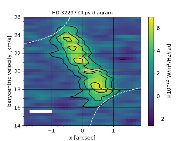
Figure 2: Position-velocity diagram of the C I emission. The $x$ coordinate runs along the major axis of the disk. Contours are drawn at intervals of 3$\sigma$. The spectro-spatial resolution is illustrated in the lower left by the white rectangle. The dashed curves show the tangential velocity for gas at projected distance $x$ from the star, assuming a stellar mass of 1.7 M_⊙ and an inclination of 83.6°.

3.3 Modeling of the C I emission

We proceed to constrain the spatial distribution and mass of neutral carbon by fitting models to the C I data cube. For a given model, specified by the spatial distribution of the gas and the temperature profile, we first calculate the level population and gas emission in each cell of a three-dimensional grid by assuming local thermodynamic equilibrium (LTE). We verified that LTE is a reasonable approximation by calculating the full radiative transfer in non-LTE using the LIME code (Brinch & Hogerheijde, 2010) for a model that fits the data (Fig. 4, see below). For that model, the total flux calculated in LTE was only a factor 1.3 higher than the flux from LIME. We use atomic data from the Leiden Atomic and Molecular Database (LAMDA, Schöier et al., 2005). The line emission profile is assumed to be Gaussian with a broadening parameter of 1 km s^-1. The emission is red- or blue-shifted according to the radial velocity (due to Keplerian rotation) of each grid cell. Then, the model is ray-traced as described in Cataldi et al. (2014) to account for optical depth. The resulting model cube is convolved in the spatial and spectral dimension to match the resolution of the data, and finally multiplied by the primary beam.

Short of a detailed heating-cooling analysis, we simply assume that the gas kinetic temperature behaves similarly as the local blackbody and varies with radial distance $r$ as $T(r)=T_{100}\sqrt{(100\,\mathrm{au})/r}$, where $T_{100}$ is a normalization constant obtained from the fit. The gas vertical scale height is given by (e.g. Armitage, 2009)

$$H(r)=\sqrt{\frac{kTr^{3}}{\mu m_{p}GM_{*}}}$$ (1)

where $k$ is the Boltzmann constant, $\mu$ the mean molecular weight, $m_{p}$ the proton mass, $G$ the gravitational constant and $M_{*}$ the stellar mass. We assume $\mu=14$ (gas mass dominated by carbon and oxygen, Kral et al., 2017), although $\mu$ might be higher since the CO mass in HD 32297 is large. The assumptions on the temperature and molecular weight should introduce only minor errors into our results.

We follow Kral et al. (2019) and consider a Gaussian surface density profile for neutral C:

$$\Sigma_{\mathrm{C^{0}}}(r)=\Sigma_{0}\exp\left(-\frac{(r-r_{0})^{2}}{2\sigma_{r}^{2}}\right)$$ (2)

where $\Sigma_{0}$ is the surface density at $r=r_{0}$ and $\sigma_{r}$ describes the radial width of the ring-like mass distribution. The number density of neutral carbon is then given by

$$n_{\mathrm{C^{0}}}(r{\color[rgb]{0,0,1},z})=\frac{\Sigma_{\mathrm{C^{0}}}(r)}{\sqrt{2\pi}Hm_{\mathrm{C}}}\exp\left(-\frac{z^{2}}{2H^{2}}\right)$$ (3)

where $z$ is the distance from the mid-plane and $m_{\mathrm{C}}$ the mass of a C atom.

We use a Markov chain Monte Carlo (MCMC) method implemented by the emcee package (version 2.2.1, Foreman-Mackey et al., 2013) to fit the model to our data (in the image space). The correlated noise in the ALMA data is handled as described by Booth et al. (2017). The following parameters are free to vary: the disk inclination $i$, the stellar mass $M_{*}$, the stellar radial velocity $v_{*}$, the ring location $r_{0}$, the ring width $\sigma_{r}$, the total mass of neutral carbon $M_{\mathrm{C^{0}}}$ and the temperature normalisation $T_{100}$. In addition, we also fit for astrometric offsets of the disk center, $\Delta x$ and $\Delta z$, which are parallel and perpendicular to the mid-plane respectively. For each parameter $\theta$, we assume uninformative priors, either with a location invariant density ($\pi(\theta)=\mathrm{const}$) or a scale invariant density ($\pi(\theta)\propto\theta^{-1}$), over the range given in Table 1. The position angle is fixed to 48.5$\arcdeg$ as determined in Appendix A. The MCMC is run for 1500 steps with 200 walkers. We discarded the first 200 samples of each walker. Table 1 shows derived parameters (50th percentile) together with error bars (16th and 84th percentile). Figure 3 shows the posterior distribution of selected parameters. We note that the temperature is not well constrained by our data. This reflects the fact that the fractional population of the transition’s upper level peaks at $\sim$30 K and then stays approximately constant for higher temperatures. The relation between the mass and the temperature is governed by the level population, as expected for an optically thin gas. The derived inclination of $77.9\arcdeg^{+1.7}_{-1.5}$ is lower than previously derived values from dust observations with ALMA ($83.6\arcdeg^{+4.6}_{-0.4}$, MacGregor et al., 2018) or from scattered light ($\sim$88°, Boccaletti et al., 2012; Currie et al., 2012). The origin of this discrepancy is unclear, but one possibility is an asymmetry in the disk that our model does not account for. We run an additional MCMC simulation with a fixed inclination of 88°and verified that the results for the other parameters do not change. In Fig. 4, we present the fit with the highest posterior probability in our chain. No strong residuals are left, suggesting that our model is a good representation of the true gas distribution. This model has a peak optical depth of 0.2 along the line of sight.

We note that the calibration uncertainty, not included in the MCMC fit, might introduce some additional uncertainty in the fitted parameters.

In summary, the C⁰ gas distribution can be fit with a ring centered at $\sim$110 au with a FWHM of $\sim$80 au. In Appendix B, we also explore fitting the data using power-law models, to accommodate the possibility that the gas has spread into a broad disk. Our results there confirm that the gas is indeed distributed in a ring-like geometry. In Appendix C, we use a simple ionisation calculation to confirm that our model is consistent with the C II emission detected by Donaldson et al. (2013).

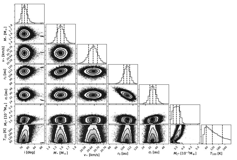
Figure 3: Posterior distributions for selected parameters of the Gaussian ring model. The vertical dashed lines indicate the 16th, 50th and 84th percentile.

Figure 4: The Gaussian ring model with the highest posterior probability. The top row shows the moment 0 and the bottom row the pv diagram. The columns show the data, the model and the residual (data minus model, with contours in steps of 3$\sigma$) respectively. The parameter values for this model are as follows: $i=77.4$°, $r_{0}=108$ au, $\sigma_{r}=36$ au, $T_{100}=76$ K, $M_{\mathrm{C^{0}}}=3.4\times 10^{-3}$ M_⊕, $M_{*}=1.6$ M_⊙, $v_{*}=20.7$ km s^-1, $\Delta x=-0.06$″, $\Delta y=0.04$″.

Table 1: Fitted parameters for the Gaussian ring model (section 3.3) and the double power law model (Appendix B). The parameters $\beta_{\mathrm{in}}$ and $\beta_{\mathrm{out}}$ are restricted to the double power law model.

Parameter	value		unit	prior	range
	Gaussian	DPL
$i$	$77.9^{+1.7}_{-1.5}$	$78.0^{+1.8}_{-1.5}$	deg	loc	[65,90]
$r_{0}$	$109^{+3}_{-4}$	$129^{+8}_{-11}$	au	loc	[30,200]
$\sigma_{r}$	$35.4^{+3.8}_{-3.5}$	-	au	sca	[0,100]
$\beta_{\mathrm{in}}$	-	$1.5^{+1.1}_{-0.6}$	-	loc	[-10,10]
$\beta_{\mathrm{out}}$	-	$-7.4^{+1.5}_{-1.6}$	-	loc	[-10,10]
$T_{100}$	$117^{+98}_{-60}$	$125^{+101}_{-64}$	K	sca	[10,300]
$M_{\mathrm{C^{0}}}$	$3.5^{+0.2}_{-0.2}$	$3.6^{+0.2}_{-0.2}$	10-3 M⊕	sca	[0,1000]
$M_{*}$	$1.59^{+0.05}_{-0.05}$	$1.59^{+0.05}_{-0.05}$	M⊙	sca	[1,3]
$v_{*}$	$20.67^{+0.04}_{-0.04}$	$20.67^{+0.04}_{-0.04}$	km s-1	loc	[18,22]
$\Delta x$	$-0.06^{+0.01}_{-0.01}$	$-0.06^{+0.01}_{-0.01}$	arcsec	loc	[-0.75,0.75]
$\Delta z$	$0.04^{+0.01}_{-0.01}$	$0.04^{+0.01}_{-0.01}$	arcsec	loc	[-0.75,0.75]

4 Model for gas production and destruction

With the observations of CO (MacGregor et al., 2018; Moór et al., 2019) and carbon (this work) at hand, we can now attempt to model the history of gas production. In the simplest story, two parameters describe this history: the event time, when gas production began, and the CO gas production rate. The value for the event time could be compared with the system age to infer something about the origin of the debris disk, and the CO production rate might be compared with the dust production rate to constrain the composition of the planetesimals. Naively, one expects the CO production rate to be a fraction of the dust mass loss rate (5.2 M_⊕ Myr^-1, Moór et al., 2019), reflecting the fractional CO content of the gas-producing bodies (typically assumed to be $\sim$10%, as suggested by outgassing solar system comets, Huebner, 2002). Our detailed modelling below suggests that a significantly higher CO production rate is required to explain the observed C and CO masses.

By using an ATLAS9 model tailored to HD 32297, we find that the CO photodissociation and C ionisation rates are dominated by the ISRF beyond $\sim$12 au from the star. This allows us to ignore stellar radiation.

To put the following model into context, we first make a simple order-of-magnitude estimate for the event time. We assume that CO molecules are photo-dissociated in the two surface layers of the disk by the ISRF without abatement, down to a column density of $N_{\mathrm{CO}}=10^{15}$ cm^-2 (behind such a column density, the dissociation rate is reduced by a factor 0.4 due to self-shielding, Visser et al., 2009). This implies a total CO destruction rate of $D_{\rm CO}=2\pi r_{0}\Delta r(2N_{\mathrm{CO}})m_{\mathrm{CO}}/(240\mathrm{yr})\sim 0.8\,M_{\oplus}/$Myr (where $m_{\mathrm{CO}}$ is the mass of a CO molecule, $r_{0}=110$ au and $\Delta r=80$ au are from the the Gaussian ring model, (table 1) and the CO lifetime is 240 yr, i.e. twice the unshielded lifetime since half of the ISRF is blocked by the disk for molecules on the surface). To accumulate the observed C⁰ mass of $M_{\mathrm{C}^{0}}\approx 3.5\times 10^{-3}$ M_⊕ (table 1) will require a timescale of

$$t_{0}\approx\frac{M_{\mathrm{C}^{0}}}{(12/28)D_{\rm CO}}\sim 10^{4}\,{\rm yr}.$$ (4)

Compared to the system lifetime, this is a surprisingly short timescale. As our model below shows, additional shielding of CO by carbon is unable to explain the short duration of the production time we derive here. Instead, the removal of carbon atomic gas by dust grains might alleviate the discrepancy between a longer production time and the low observed carbon mass.

4.1 Time Evolution Model

Here, we present a simple model to capture a few main processes that affect the time evolution of CO and carbon. This includes UV shielding of CO by carbon, CO self-shielding and carbon removal (e.g. via re-capture by dust grains). The shielding aspect of our model is similar in spirit to that in Kral et al. (2019); Moór et al. (2019); Marino et al. (2020), but differs (substantially) in the treatment of shielding.

We consider only one radial zone of well-mixed gases and discard the effect of gas removal by viscous spreading (as is justified here, see section 5.2). The CO mass evolves as

$$\frac{dM_{\rm CO}}{dt}=P_{\mathrm{CO}}-D_{\mathrm{CO}},$$ (5)

where $P_{\mathrm{CO}}$ is the CO production rate by the debris ring and $D_{\mathrm{CO}}$ the CO photo-destruction rate. CO is produced in a collisional cascade among the debris. Intuitively, we might expect some time dependence of $P_{\mathrm{CO}}$ such as a gradual decrease due to the collisional evolution of the disk (Marino et al., 2020). However, for simplicity, we assume a constant CO production rate. The carbon mass evolves with time as

$$\frac{dM_{\rm C}}{dt}=\frac{12}{28}D_{\rm CO}-\frac{M_{\mathrm{C}}}{\tau_{\mathrm{C}}}$$ (6)

The second term on the right-hand-side models a carbon sink (e.g. capture onto dust grains). To convert $M_{\mathrm{C}}$ into masses of neutral and ionised carbon, a constant ionisation fraction of 0.2 is assumed (appendix C).

In contrast to Kral et al. (2019), we obtain the photo-dissociation rate ($D_{\mathrm{CO}}$) using photon counting. The probability that a given ISRF photon either ionises C⁰ or dissociates CO is given by

$$f_{1}=1-\exp(-\tau_{\mathrm{C^{0}}}-\tau_{\mathrm{CO}})=1-\exp(-\tau_{\mathrm{tot}})$$ (7)

where the optical depth $\tau_{x}(\lambda)=N_{x}\sigma_{x}(\lambda)$ with $N_{x}$ the vertical column density and $\sigma_{x}$ the wavelength-dependent cross section. Under our assumption of perfect mixing, the fraction of these photons dissociating CO is

$$f_{2}=\frac{n_{\mathrm{CO}}\sigma_{\mathrm{CO}}}{n_{\mathrm{C^{0}}}\sigma_{\mathrm{C^{0}}}+n_{\mathrm{CO}}\sigma_{\mathrm{CO}}}=\frac{\tau_{\mathrm{CO}}}{\tau_{\mathrm{tot}}}$$ (8)

where $n$ denotes number density. Let $\phi_{\nu}$ be the number of ISRF photons hitting the disk per unit time, per unit frequency, per unit area (taken from Draine, 1978). The photo-destruction mass rate for CO is

$$D_{\mathrm{CO}}=m_{\rm CO}\int\phi_{\nu}Af_{1}f_{2}\,d\nu$$ (9)

where $A=2\pi r_{0}\Delta r$ is the surface of the disk. An alternative derivation of this equation is given in appendix E.

Equation 9 can be used to derive an upper limit on the CO destruction rate. We assume $f_{1}=f_{2}=1$ for any frequency $\nu$ where $\sigma_{\mathrm{CO}}(\nu)>0$, i.e., no photon that could potentially destroy a CO molecule is lost. This leads to $D_{\mathrm{CO}}^{\mathrm{max}}\sim 50$ M_⊕ Myr^-1 (with $r_{0}=110$ au and $\Delta r$=80 au). In the case that $P_{\mathrm{CO}}>D_{\mathrm{CO}}^{\mathrm{max}}$, no steady state is possible.

We extend our model to also include the evolution of ¹³CO and C¹⁸O. This is easily achieved by replacing $\tau_{\mathrm{CO}}$ in equation 7 by $\tau_{\mathrm{{}^{12}CO}}+\tau_{\mathrm{{}^{13}CO}}+\tau_{\mathrm{C^{18}O}}$. Then, the masses of the isotopologues are evolved the same way as ¹²CO. The wavelength-dependent cross sections of the different isotopologues only overlap partially. Therefore, the lower abundance isotopologues are more readily photodissociated since their self-shielding is weaker. This effect is called isotopologue selective photodissociation. It increases the ratios of ¹²CO/¹³CO and ¹²CO/C¹⁸O compared to the ISM ratios, and is naturally taken into account by our model.

The cross-sections for CO photo-dissociation were provided by A. Heays (private communication) and are based on Visser et al. (2009), while the ionization cross section $\sigma_{\mathrm{C}}$ is from the database of ’Photodissociation and photoionization of astrophysically relevant molecules’ (hereafter PPARM, Heays et al., 2017); $\sigma_{\mathrm{C}}$ is essentially constant ($\sim$1.6$\times 10^{-17}$ cm²) over the wavelength range where CO photodissocation happens (Rollins & Rawlings, 2012).

We note that the Kral et al. (2019) model has a different approach to the calculation of the CO destruction rate and we argue that they under-estimate it in the shielded regime. In their model,

$$D_{\mathrm{CO}}=M_{\rm CO}\times\chi_{0}\times S(N_{\mathrm{CO}})\times\exp(-N_{\mathrm{C^{0}}}\sigma_{\mathrm{C^{0}}})$$ (10)

where $\chi_{0}$ is the unshielded ISRF photodissociation rate and $S(N_{\rm CO})$ is the reduction on $\chi_{0}$ due to CO self-shielding under a column density $N_{\rm CO}$ (Visser et al., 2009). However, equation 10 is the dissociation rate for a CO molecule that sits behind the full column densities of C and CO. First, such a model ignores the CO dissociation in the shielding layer and therefore over-estimates the effect of shielding. In contrast, our model predicts higher CO destruction rates because even if the mid-plane is strongly self-shielded, ISRF photons are still used to dissociate CO in the higher layers of the disk. Second, the Kral et al. (2019) model also implicitly assumes that C forms a separate layer at the surface of the disk, as expressed by the exponential term in equation 10. This maximises the effect of C shielding. In contrast, in our model, C and CO are well-mixed. Observations of C I that resolve the vertical structure are needed to decide which prescription is a better representation of a real disk.

Next, we consider carbon condensation onto dust grains. We estimate the total dust cross section by adopting a dust mass of 0.57 M_⊕ (MacGregor et al., 2018), a minimum grain diameter equal to the blowout limit ($\sim$10 $\mu$m), a maximum grain diameter of 1 mm and a power-law size distribution with index -3.5. Adopting $T=100$ K and $n_{\mathrm{C}}=370$ cm^-3 (from our Gaussian ring model fit), we find that the mean free time of a C atom before colliding with a dust grain is $\sim$5000 yr. Grigorieva et al. (2007) also estimated the recondensation of water onto dust grains. By adapting their equation 17 to C, we find that all C is recondensed on a timescale of $\sim$8000 yr. So this process might be important. Although collisions between C atoms and the grains have nearly unity sticking coefficient (e.g. Hollenbach & Salpeter, 1970; Leitch-Devlin & Williams, 1985), thermal desorption might remove them again quickly. In the later discussion, we consider this more in detail and also discuss whether the accreted atoms can form fresh CO (section 5.1).

In the following, we leave the removal timescale $\tau_{\mathrm{C}}$ as a free parameter in our model. Figure 5 illustrates three examples of our model for different rates of CO production without and with removal of carbon (taking $\tau_{\mathrm{C}}=\infty$ and 5000 yr, respectively). For these models, we fixed $r_{0}=110$ au and $\Delta r=80$ au. We find that without C removal, once either C⁰ shielding or CO self-shielding is significant, both C and CO rise linearly and the C⁰/CO ratio remains constant. When the CO production rate is low, C shielding is necessary before CO can survive rapid destruction. This explains the initial delay in its mass rise (left panel). Later on, both masses grow linearly, with a fixed fraction of the freshly made CO being turned into C. The ratio of C⁰/CO is above unity. In comparison, in the models with a high CO production rate (middle and right panels), even from the very beginning, CO self-shielding is already significant. We still observe a linear growth in both masses, but the C⁰/CO mass ratio is consistently below unity. On the other hand, removal of C gas allows the system to settle to a steady state in which the removal of C is balanced by its production from CO dissociation. We note that the C⁰/CO ratio decreases with increasing CO production rate, regardless of whether C is removed or not. For HD 32297, the observed C⁰/CO$\ll 1$ suggests that a large CO production rate will be required to explain the observations.

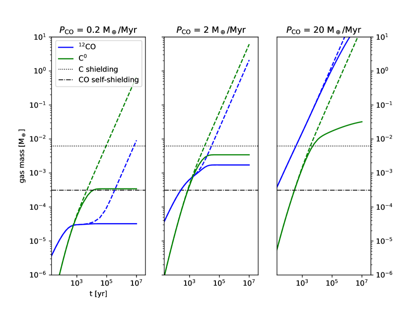
Figure 5: Evolution of the CO and C⁰ mass for different CO production rates (rising from the left to the right). The solid lines are for models with $\tau_{\mathrm{C}}=5000$ yr and the dashed lines for models without C removal ($\tau_{\mathrm{C}}=\infty$). The horizontal lines indicate the masses at which C⁰ shielding (dotted) or CO self-shielding (dash-dotted) become significant, i.e. the dissociation rate in the midplane is reduced by a factor 0.3. For models with $\tau_{\mathrm{C}}=\infty$, shielding allows both masses to rise linearly with time, and the mass ratio of C⁰/CO remains constant. In contrast, models with C removal settle to a steady state within the simulated time span, except for the highest CO production rate considered here (right panel).

4.2 Applying to HD 32297

Here, we apply our above model to the specific case of HD 32297. The planetesimal belt is observed to have a width of $\sim$40 au if we ignore the ’halo component’ (MacGregor et al., 2018). Thus, the C gas with its FWHM of $\sim$80 au is observed to be mildly more spread out. For simplicity, we ignore this difference and fix the width of the gas disk to 80 au.

Our model contains two unknowns: the event time ($t_{0}$) at which CO (and presumably dust) production commenced, and the CO production rate ($P_{\rm CO}$). We aim to reproduce two observables: the C⁰ mass ($3.5\times 10^{-3}$ M_⊕) and the mass of C¹⁸O ($1.4\times 10^{-4}$ M_⊕, Moór et al., 2019). We use the C¹⁸O mass because the main component of the CO gas, ¹²CO, is optically thick and its mass cannot be determined accurately. We also ignore ¹³CO as it may be optically thick as well.

4.2.1 Steady-state solution

We first consider the case where the system described by equations 5 and 6 is in a steady state. A steady state solution only exists if C is removed, i.e. $\tau_{\mathrm{C}}$ is finite.

In steady state, destruction rates equal production rates: $P_{\mathrm{{}^{y}C^{z}O}}=D_{\mathrm{{}^{y}C^{z}O}}$ with ^yC^zO a specific CO isotopologue. The destruction rate $D_{\mathrm{{}^{y}C^{z}O}}$ can be calculated if masses of all CO isotopologues and of C⁰ are known (equation 9). However, as mentioned above, only the C¹⁸O mass is well measured (Moór et al., 2019). To proceed, we first compute the ¹²CO and ¹³CO masses using the measured C¹⁸O mass, assuming ISM ratios: $\mathrm{{}^{13}CO}/\mathrm{{}^{12}CO}=1.4\times 10^{-2}$ and $\mathrm{C^{18}O}/\mathrm{{}^{12}CO}=1.8\times 10^{-3}$ (Wilson, 1999). We then calculate the destruction rate of each isotopologue using equation 9. By the steady state assumption, these destruction rates are equal to the production rates. We find that the production rates of ¹³CO and C¹⁸O (relative to ¹²CO) are enhanced by a factor $\sim$6 relative to the ISM ratios. This would imply that the gas-producing solids are enhanced in ¹³CO and C¹⁸O. However, isotopologue ratios in solar system comets show ¹²C/¹³C and ¹⁶O/¹⁸O ratios broadly similar to the ISM ratios (e.g. Hässig et al., 2017; Altwegg et al., 2019, and references therein). This motivates us to search for values of the ¹²CO and ¹³CO masses that imply CO production rate ratios consistent with ISM ratios. We find $M_{{}^{12}\mathrm{CO}}=1.6$ M_⊕ and $M_{{}^{13}\mathrm{CO}}=1.5\times 10^{-3}$ M_⊕, i.e., we require a ¹²CO/C¹⁸O mass ratio enhancement by a factor 20 relative to the ISM value. This is not unexpected, because isotopologue selective photodissociation can preferentially destroy the rarer isotopologues. The CO production rate inferred from these masses is very high, $16$ M_⊕ Myr^-1. The corresponding steady state C removal timescale (equation 6) is short: $\tau_{\mathrm{C}}\approx 700$ yr. This is a consequence of the small C⁰ mass we measure.

We note that with a CO mass as high as $1.6$ M_⊕, carbon shielding plays a relatively minor role—when neglecting the shielding contribution of neutral carbon, the CO destruction rate is increased by only $\sim$20%.

4.2.2 Full calculation

We now do not assume steady state and instead evolve a grid of models with different event times ($t_{0}$) and CO production rates ($P_{\rm CO}$) with the goal of reproducing the observed masses of C⁰ and C¹⁸O. We fix the isotopologue ratios in the gas-producing solids (i.e. the CO production rate ratios) to ISM ratios.

Our model results are presented in Figure 6. In the case of no C removal ($\tau_{\mathrm{C}}=\infty$, left panel), we find that only the combination of an extremely high CO production rate and a recent event can explain the data: $P_{\mathrm{CO}}\approx 100$ M_⊕ Myr^-1 and $t_{0}\approx 1000$ yr. As can be seen from the figure, for lower CO production rates, that model exceeds the observed C mass long before it has built up the observed C¹⁸O mass.

Figure 6 (right) shows a scenario were $\tau_{\mathrm{C}}$ is adjusted such that the observed gas masses can be explained with a steady state solution. We find $\tau_{\mathrm{C}}\sim 700$ yr is necessary, i.e. C gas needs to be removed efficiently in order to reproduce the small C mass we observe: for larger values of $\tau_{\mathrm{C}}$, the results are qualitatively similar to the $\tau_{\mathrm{C}}=\infty$ case, while for smaller values, no solution is found. Even in this scenario, the required CO production rate remains high at $\sim$15 M_⊕ Myr^-1 (as mentioned in section 4, based on the dust mass loss rate, we would expect a CO production rate of $\sim$0.5 M_⊕ Myr^-1). Steady state is reached after a few times $10^{5}$ years. The steady state CO mass is 1.3 M_⊕. These results are consistent with the steady state solution described in section 4.2.1.

In Figure 7, we show the two models that can formally explain the observed gas masses, with parameters as identified from Figure 6. As mentioned above, the first model (no removal of carbon) requires a very recent event and an extremely large CO production rate. By the time the model fits the observed C⁰ and C¹⁸O masses, the total CO mass released is $\sim$0.1 M_⊕. This model can thus be interpreted as the recent destruction of a $\sim$1 M_⊕ body with a CO fraction of 10% releasing all of its CO within 1000 yr. In the following, we focus on discussing the second model. In this latter case, the model does not give us a unique answer regarding the event time, other than that it must be greater than $\sim 10^{5}$ yr. For comparison, the system lifetime is larger than 15 Myr. The CO production rate of 15 M_⊕ Myr^-1 is in contrast with the result from Moór et al. (2019), where they found that $P_{\mathrm{CO}}\approx 3.6\times 10^{-2}$ M_⊕ Myr^-1. However, the Moór et al. (2019) model over-predicts the C⁰ mass by a factor 10 compared to our data, despite underestimating the CO break-down rate due to the different treatment of shielding (section 4.1).

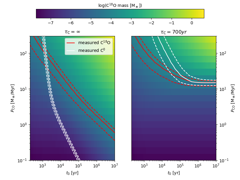
Figure 6: C¹⁸O mass (with color bar) calculated from our model as a function of CO production rate (vertical axis) and event time (horizontal axis) for a scenario without removal of C (left) and with $\tau_{\mathrm{C}}=700$ yr (right). The solid red and white lines show the parameter combinations that give rise to the observed C¹⁸O ($1.4\times 10^{-4}$ M_⊕, Moór et al., 2019) and C⁰ ($3.5\times 10^{-3}$ M_⊕, this work) masses respectively, with the dashed lines corresponding to the $\pm 3\sigma$ uncertainty ranges. The correct parameters lie where these two sets of lines intersect. In the right panel, evolution settles down to a steady state, so we lose sensitivity to the event time after $\sim 10^{5}$ yr.

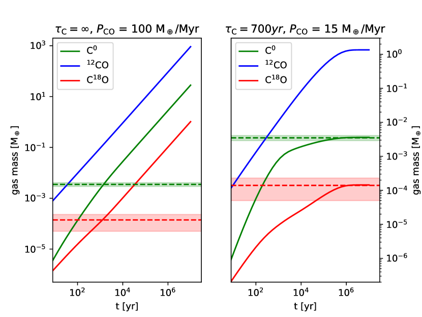
Figure 7: Evolution of models without (left) and with (right) removal of C gas that can reproduce the observed C⁰ and C¹⁸O masses (model parameters as inferred from figure 6). The horizontal dashed lines indicate the observed masses, with the shaded regions corresponding to $\pm 3\sigma$ ranges.

5 Discussion

The results of our steady state model have two obvious contradictions: the inferred CO production rate (15 M_⊕ Myr^-1) exceeds the total dust mass loss rate (5.2 M_⊕ Myr^-1; Moór et al., 2019); and the C removal timescale ($\tau_{C}=700$ yr) is shorter than what we naively estimated based on dust cross-section ($\sim$5000 yr, see section 4.1).

For a CO (and CO₂) mass fraction of $10\%$, we expect a CO production rate $\sim$30 times below what we obtain above. A number of factors may bring some relief: uncertainties on the value of dust grind-down rate can be up to a factor of 10 (Kral et al., 2019); the CO production rate may be time-dependent, as opposed to being constant as assumed here (Marino et al., 2020). But a tension remains in that our required CO production rate is higher than the total dust rate.

In the following, we discuss a new process: CO re-formation. We describe how this process could allow the CO production rate to be (much) larger than the dust grind-down rate. It could also explain the belt-like appearance of the gas disk. We then go on to discuss the inferred carbon removal time and a number of alternative removal processes. We end by discussing the implications of our results for the origin of debris disks.

5.1 Carbon removal by dust grains and CO re-formation

Here, we consider the fate of carbon atoms that collide with dust grains. We also discuss the possibility that accreted C atoms will react with O to reform CO. Although O I 63 $\mu$m emission was not detected by Herschel (Donaldson et al., 2013), we expect O to be at least as abundant as C, thanks to photodissociation of CO, CO₂ and H₂O, all of which should be present in the cometary parent bodies.

We first consider if atoms can remain on the grain or are quickly re-relased to the gas phase by thermal desorption. The rate of thermal desorption $R_{\mathrm{td}}$ depends on the binding energy $E_{i}$ (Hollenbach & Salpeter, 1970; Tielens & Hagen, 1982):

$$R_{\rm td}\approx\nu_{i}e^{-E_{d}/kT_{\rm gr}}$$ (11)

where $\nu_{i}\sim 10^{13}$ s^-1 (Tielens & Hagen, 1982) is the characteristic oscillation frequency for the atom in the lattice potential. The value of the binding energy depends on the type of interaction between the adsorbate and the surface (e.g. Tielens, 2005). Binding by van der Waals forces (physiosorption) is relatively weak (0.01–0.2 eV, Tielens, 2005), while valence bonds (chemisorption) are stronger ($\sim$1 eV). Whether adsorbed atoms are physiosorbed or chemisorbed depends on the grain properties (e.g. chemical composition, temperature; Y. Aikawa, private communication). For instance, let us assume a grain temperature of 50 K. If C is physiosorbed with a binding energy of 0.1 eV, it would be thermally desorbed in a fraction of a second. In such a case, dust grains cannot act as C sink. On the other hand, chemisorbed C can be accumulated on the grains. More studies (e.g. quantum chemical computations such as in Shimonishi et al., 2018) are needed to determine the binding energy of C (and O) on dust grains.

Next, we consider the possibility that accreted C and O atoms reform CO on the dust grains. Detailed modelling to determine if and under which conditions C+O$\rightarrow$CO can proceed on the dust grains is beyond the scope of this paper. However, if the reaction proceeds, it has interesting consequences. CO is then continuously recycled: it is released from grains, photo-dissociated by the ISRF, C and O re-accreted onto grains, CO re-formed rapidly, and re-released into space. In this picture, as long a certain amount of CO is injected as gas at some point, there is no need for fresh CO production. The CO production rate that we infer would simply be a result of CO reformation. Consider a C mass of $3\times 10^{-3}$ M_⊕ and a removal time of $\tau_{\mathrm{C}}=700$ yr. This yields the rate of CO reformation, $\sim 10$ M_⊕ Myr^-1, as we obtain above. It is not necessary for the CO production rate to be limited by the dust grind-down rate. CO re-formation would also explain why the carbon gas is concentrated into a narrow radial belt—all gas components have been released so recently that they did not have time to spread viscously.

We experimented with a modified version of our model with an additional CO source term equal to $28/12M_{\mathrm{C}}/\tau_{\mathrm{C}}$, i.e. each removed C atom is immediately converted to a CO molecule. Then, the observed C and CO masses can indeed be reproduced with much smaller CO production rates ($P_{\mathrm{CO}}\lesssim 1$ M_⊕ Myr^-1) compared to our standard model.

5.2 Other C removal processes

While consideration of dust capture yields a carbon removal time of $\tau_{C}\sim 5000$ yr (section 4.1), our model requires a much shorter $\tau_{c}\sim 700$ yr, in order to explain the low C⁰ mass we infer from the ALMA observations. We consider a number of alternative carbon removal mechanisms, but do not find a satisfactory solution to this problem at the moment.

1. Gas accretion into the star appears ineffective in HD 32297, as the gas ring appears narrow, not radially spread into an accretion disk. Indeed, our modeling of the C I emission suggests that the gas is distributed in a ring that is only mildly broader than the dust ring.

2. Can one or several planets inward of the dust belt prevent the formation of an accretion disk by accreting gas themselves? So far, no giant planets have been found in direct imaging searches around HD 32297 (Boccaletti et al., 2012; Rodigas et al., 2014; Bhowmik et al., 2019). In the most recent study, Bhowmik et al. (2019) exclude the presence of planets with 2.5–6 Jupiter masses at projected distances beyond $\sim$80 au. However, because of the edge-on geometry of the disk, planets might be hiding close to the line of sight towards the star. Furthermore, Marino et al. (2020) found that smaller, currently undetectable Neptune-class planets can be sufficient to accrete gas.

3. Marino et al. (2020) recently suggested that C might become undetectable as it viscously spreads outwards to regions at larger radii with lower surface density. More detailed modeling is needed to test this proposition. Naively, one might expect this to be less of a problem for an edge-on disk like HD 32297 where the column density along the line of sight is high compared to a face-on disk. This scenario would also imply efficient spreading and thus would again require a mechanism to prevent the formation of an inward accretion disk (see the previous point).

4. What about carbon removal by gas phase chemistry? Consulting the chemical network and reaction rates relevant for proto-planetary disks, as compiled by Glover et al. (2010), we find that the most probable pathway for carbon removal is the following reaction

   $$\mathrm{OH}+\mathrm{C}\rightarrow\mathrm{CO}+\mathrm{H},$$ (12)

   with a reaction rate of $k=10^{-10}$ cm³ s^-1 (similarly, OH + C⁺ $\rightarrow$ CO⁺ + H has $k=7.7\times 10^{-10}$ cm³ s^-1). Thus, to match our required C removal timscale of $\tau_{\mathrm{C}}=700$ yr, we would require $n_{\mathrm{OH}}=(\tau_{\mathrm{C}}k)^{-1}=0.5$ cm^-3. The OH molecules are likely the results of water photo-dissociation, and they are highly vulnerable to UV photo-dissociation. So for this channel to be effective in removing carbon gas, one requires a copious amount of water production. We encourage more detailed modeling to assess how chemistry influences the evolution of debris disk gas.

5. Can carbon gas spontaneously condense into solid form, without the assistance of dust grains? The low-temperature phase diagram of carbon (see e.g. Jaworski et al., 2016) shows that the vapour pressure for condensation of gaseous atomic C into solid state at the relevant temperature range is orders of magnitude below the gas pressure in the disk. However, typical condensation requires the presence of seed nuclei. These nuclei ought to be scarce as they are quickly removed by the radiation pressure from the A-star (Weingartner & Draine, 2001), although sufficient amounts of gas could lengthen their residence time.

Another possible solution might be to assume a CO production that is enhanced in isotopologues. For instance, we experimented with a model where the production rate of ¹³CO and C¹⁸O, relative to ¹²CO, is enhanced by a factor of 10 from the ISM ratio. At steady state, we require a CO production rate of 5 M_⊕ Myr^-1, and a carbon removal time of $\tau_{c}\sim 2000$ yr, more similar to the 5000 yr inferred in section 4.1.

5.3 Other Uncertainties

The conclusions we draw from our modelling rely heavily on our main observational result: the low mass of neutral carbon. How robust is this mass measurement? Could it be that the small error bars (see Table 1) derived from the MCMC modelling are underestimating the real uncertainty? One scenario that could increase the C⁰ mass estimate is a low kinetic temperature. This could lead to a high optical depth, allowing for an arbitrarily high C⁰ mass, in principle. We discuss this possibility in appendix D. Overall, we believe that our mass error-bars are reasonable.

Regarding UV shielding, we can exclude the possibility of another shielding agent. Other than carbon and CO, there are no promising molecules or atoms in the PPARM database that have the required high cross-section at the relevant wavelengths to provide shielding.

Next, the strength of the ISRF may be somewhat uncertain. Very few direct observations exist (e.g. Henry, 2002), and there may also be some spatial variations caused by proximity to massive stars (e.g. van Dishoeck, 1994). A weaker ISRF than the canonical value assumed here would reduce the CO destruction rate, and correspondingly, the inferred CO production rate.

Finally, our model assumes that CO and C are well-mixed. When instead assuming that all C is concentrated at the surface of the disk (this configuration maximises C shielding), the derived CO production rates and C removal timescales only change by a factor of $\sim$2. This reflects the modest shielding by the small measured C mass. For larger C masses, the difference can be more dramatic.

5.4 Implications for Debris Disks

When was the dusty disk around HD 32297 produced? Is it as old as the star, or is it the result of a recent catastrophic event? What is the total mass of the underlying planetesimal belt? Our model without C removal requires a catastrophic event 1000 yr ago, i.e. the CO gas was released within an orbital timescale. In such a scenario, the symmetric appearance of the disk in CO and C I is challenging to explain. On the other hand, our steady state model cannot give a unique answer to the event time, so we look to other evidence for guidance.

If the CO gas has been steadily produced over a long timescale, it and its descendants (carbon and oxygen gas) ought to have viscously spread out and eventually accreted onto the star. For a gas belt of width $\Delta r$, and an $\alpha$ parameter of $0.01$, as likely appropriate for gaseous debris disks (Kral & Latter, 2016), the time required to double the radial width is of order

$$t\sim\frac{(\Delta r)^{2}}{\alpha c_{s}H}\sim 10^{6}\,{\rm yr}\,\left(\frac{\Delta r}{40\,{\rm au}}\right)^{2}.$$ (13)

However, our modeling of the C I emission (section 3.3) suggests that the gas is distributed in a ring that is only mildly broader than the dust ring, indicating that there is insignificant radial spreading around HD 32297, since gas production started. Could this imply that the event time is shorter than the system lifetime ($\geq 15$ Myrs)? The answer is no. Any newly outgassed CO is necessarily concentrated near the grains’ orbits. It is photo-dissociated within a time short compared to the above spreading time (mean lifetime in our model is $0.1$ Myr). And its descendant, the C gas, is rapidly removed ($\tau_{\mathrm{C}}\sim 700$ yr). So no radial spreading is allowed in the steady state model.

The high CO production rate that we obtain ($\sim 15$ M_⊕ Myr^-1) can in principle place a constraint on the event time, since it is not sustainable over a long period of time. However, this is not true if CO recycling occurs. In the latter case, even if gas production started right after the dispersal of the protoplanetary disk, the minimum CO required is still only of order M_⊕ (the current CO gas mass), roughly the amount of CO contained by a comet belt of some 10 M_⊕. This total mass is consistent with the estimates based on the gradual luminosity evolution of debris disks (e.g. Shannon & Wu, 2011).

Previously, Cataldi et al. (2018) concluded that the debris disk around $\beta$ Pic has to be produced recently. In that system, the ¹²CO emission is optically thin and the CO mass can be directly measured (Matrà et al., 2017b). It is at least three orders of magnitude lower than that in HD 32297, while the carbon masses are comparable. Moreover, both CO and carbon are distributed in a highly asymmetric, radially confined ring (Cataldi et al., 2018). The low C and CO masses imply little shielding and the CO lifetime is as short as $\sim$50 yr, or a CO destruction rate of $0.6$ M_⊕ Myr^-1. Assuming that the low amount of C is the integrated result of this destruction rate, Cataldi et al. (2018) concluded that carbon can be accumulated in a time as short as $\lesssim 10^{4}$ yr. However, this picture of a short event time would drastically be changed if C is removed. In such a case, the low carbon mass no longer places a constraint on the event time directly.

Besides $\beta$ Pic and HD 32297, there are currently two other debris disks with resolved CO and C I observations: HD 131835 and 49 Ceti. For HD 131835, Kral et al. (2019) derived $r_{0}=90$ au, $\Delta r=70$ au and a C⁰ mass between $2.7\times 10^{-3}$ M_⊕ and $1.2\times 10^{-2}$ M_⊕. The CO mass is estimated at $0.04$ M_⊕ (Moór et al., 2017; Kral et al., 2019). The spatial distribution of the gas is uncertain and there remains the possibility that an accretion disk has formed (Kral et al., 2019). For 49 Ceti, the dust belt is concentrated around $r_{0}\sim 100$AU, with a width $\Delta r\sim 80$ au (the double power law model of Hughes et al., 2017), while the carbon mass is $M_{\mathrm{C^{0}}}=3\times 10^{-3}$ M_⊕ (assuming optically thin emission; A. Higuchi, private communication 2019) and the CO mass (if ISM ratios apply) $(1.11\pm 0.13)\times 10^{-2}$ M_⊕ (Moór et al., 2019). Hughes et al. (2017) found that the CO observations are well described by a model where the surface density increases with radius between $\sim$20 and $\sim$220 au, suggesting that an accretion disk is unlikely. Both disks might be qualitatively explained by a scenario similar to HD 32297 (figure 7 right).

Recently, Marino et al. (2020) presented a population synthesis study by coupling the secondary gas production model by Kral et al. (2019) with a dust collisional evolution model (i.e. the dust grind down rate, and thus CO production, decay with time). While they find agreement with measured CO masses, their model tends to overpredict the masses of neutral C, although they get better agreement by assuming that C beyond the belt location is not detectable in observations. This result seems analogous to our finding that the small C mass around HD 32297 is difficult to reproduce with a CO production rate derived from the dust mass loss rate.

6 Summary

In this work, we present resolved ALMA observations of C I emission at 492 GHz from the HD 32297 debris disk. The data are used to investigate the age and the gas production rate of the disk. Our results can be summarized as follows:

1. The spatial distribution of neutral carbon can be modelled by a Gaussian ring surface density profile centered at 110 au with a FWHM of 80 au. A double power law model can also fit the data satisfactorily. The mass of neutral carbon is $(3.5\pm 0.2)\times 10^{-3}$ M_⊕.

2. We attempt to explain the gas-rich debris disk around HD 32297 by secondary gas production. We present a model where CO is produced at a fixed rate and destroyed by photodissociation, which in turn produces carbon. The carbon can itself be removed (e.g. by capture onto dust grains). The model includes CO self-shielding and CO shielding by neutral carbon.

3. We aim to reproduce both the C⁰ mass determined in this work and the C¹⁸O mass. Without removal of C gas, our model requires that 0.1 M_⊕ of CO were released over the past 1000 yr, maybe in the catastrophic destruction of a planetary body. However, the absence of asymmetries in the C I and CO data might be hard to explain in such a scenario. For a steady state solution, the model requires very efficient removal of C ($\tau_{\mathrm{C}}\sim 700$ yr). Even in that case, the CO production rate remains high at $\sim$15 M_⊕ Myr^-1, exceeding the dust mass removal rate. For such high CO production rates, shielding by C is negligible compared to CO self-shielding. The total CO mass inferred from our model in steady state is 1.6 M_⊕.

4. The existence of a steady-state solution means that the event time (the time when dust and gas production commence) is not constrained in our model.

5. We consider the fate of C⁰ atoms that collide with grains. Depending on the binding energy, they may stick to the grains. We propose that they might reform CO (with incoming O atoms) that is re-released to the gas phase. This would lead to a continuous recycling of CO. Such a picture would explain the high CO production rate, and the belt-like gas disk, despite viscous spreading.

It is desirable to verify our model and to extend it to other debris disks with gas observations. In particular, the idea of CO re-formation needs to be tested, as it might be an important process in gas-rich debris disks. And there still exists a discrepancy between our inferred carbon removal timescale and that estimated based on dust grain capture.

Appendix A Position angle of the disk

The position angle (PA) of the HD 32297 disk was measured from ALMA Band 6 continuum data by MacGregor et al. (2018). They found $47.9\arcdeg\pm 0.2\arcdeg$, consistent with measurements from scattered light observations (e.g. Asensio-Torres et al., 2016). We measure the PA from our continuum image (Fig. 1, right). For a given trial PA $\phi$, we first rotate the disk by an angle $\pi-\phi$ to align it with the horizontal axis. Then, we use three different methods to grade the trial PA:

1. We consider the flux inside a $2\arcsec\times 0.4\arcsec$ box (this is slightly smaller than the extent of the disk) centered at the stellar position. We search for the PA that maximizes the flux.

2. We follow Asensio-Torres et al. (2016) and mirror the rotated image along the vertical axis. Then, the mirror image is subtracted from the rotated image to get a residual image. We search for the PA $\phi$ that minimizes the residuals.

3. We follow Matrà et al. (2017b) and fit a Gaussian to each vertical row of pixels in the rotated image. The centers of the Gaussians define the spine of the disk. We perform a linear fit to the spine. We search for the PA that produces a linear fit to the spine with a slope closest to zero.

We consider trial PAs between $43\arcdeg$ and $53\arcdeg$ with steps of $0.2\arcdeg$, giving us an estimate of the PA for each of the three methods. In order to estimate errors, we employ a Monte Carlo method and resample the data 1000 times by adding noise to our image and repeating the fit (e.g. Andrae, 2010). The noise in our image is correlated. We extend the method described in Appendix A of Cataldi et al. (2014) to two dimensions to produce synthetic correlated noise that can be added to our image. We find PA values of $49.2\arcdeg\pm 1.0\arcdeg$, $48.2\arcdeg\pm 1.3\arcdeg$ and $48.2\arcdeg\pm 1.0\arcdeg$ for each of the above methods respectively. Taking the mean and combining the errors quadratically yields a final estimate of $48.5\arcdeg\pm 0.6\arcdeg$, consistent with the value derived by MacGregor et al. (2018). We repeat the analysis for the C I moment 0 map (Fig. 1, left) and find values consistent with the PA estimated from the continuum.

Appendix B Power law models

We also fit the double power law proposed by Kral et al. (2019) to our data. The surface density of neutral carbon is given by

$$\Sigma_{\mathrm{C^{0}}}(r)=\begin{cases}\Sigma_{0}\left(\frac{r}{r_{0}}\right)^{\beta_{\mathrm{in}}},&\text{if }r<r_{0}\\ \Sigma_{0}\left(\frac{r}{r_{0}}\right)^{\beta_{\mathrm{out}}},&\text{if }r>r_{0}.\end{cases}$$ (B1)

The fitted parameters remain the same as for the Gaussian ring, except that $\sigma_{r}$ is replaced by $\beta_{\mathrm{in}}$ and $\beta_{\mathrm{out}}$. Table 1 lists the derived parameter values. Figures 8 and 9 show the posterior distribution of selected parameters and the fit with the highest posterior probability, respectively. From the posterior probability distribution we find that the parameter $\beta_{\mathrm{in}}>1$ at the 81% confidence level, suggesting that the inner region is devoid of gas, as seen for the Gaussian ring fit. The parameter $\beta_{\mathrm{out}}$ is strongly negative, implying a sharp cutoff of the gas density at $r_{0}$.

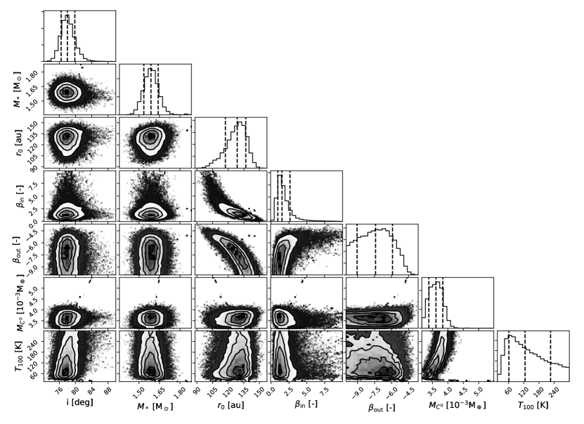
Figure 8: Posterior distributions for selected parameters of the double power law model. The vertical dashed lines indicate the 16th, 50th and 84th percentile.

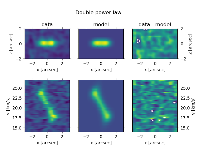
Figure 9: Same as Fig. 4, but for the double power law model. The parameter values for this model are as follows: $i=77.2$°, $r_{0}=136$ au, $\beta_{\mathrm{in}}=1.1$, $\beta_{\mathrm{out}}=-9.0$, $T_{100}=69$ K, $M_{\mathrm{C^{0}}}=3.3\times 10^{-3}$ M_⊕, $M_{*}=1.6$ M_⊙, $v_{*}=20.7$ km s^-1, $\Delta x=-0.05$″, $\Delta y=0.04$″.

In order to further test the inner extend of the disk, we fit a third model that has the same surface density as the double power law, except that no gas is present inside of a minimum radius $r_{\mathrm{min}}$. Also, since $r_{\mathrm{min}}$ and $\beta_{\mathrm{in}}>0$ have a similar effect, we force $\beta_{\mathrm{in}}$ to be negative. We find that $r_{\mathrm{min}}>60$ au at the 95% confidence level, giving further confidence that the gas is distributed in a ring-like geometry.

Appendix C Comparison to C II data

Donaldson et al. (2013) detected C II 158 $\mu$m emission towards HD 32297. We check whether our C⁰ models are consistent with this measurement. For a given model describing the distribution of neutral carbon, we calculate the ionisation in every grid cell of the model. For simplicity, we assume that the gas is optically thin to ionising radiation. This assumption is justified, because the ISRF is the dominating source of ionising photons and the typical vertical optical depth of our models to ionising radiation is only $\sim$1. Note however that, although neglected here, the optical depth of C⁰ to ionising radiation is important when considering the shielding of CO (section 4.1). Assuming that electrons are solely produced by C ionisation, the C⁺ number density is given by

$$n_{\mathrm{C^{+}}}=\sqrt{\frac{n_{\mathrm{C^{0}}}\Gamma}{\xi}}$$ (C1)

where $\Gamma$ is the ionisation rate computed using cross sections from the NORAD database (Nahar & Pradhan, 1991) and $\xi$ the recombination rate, taken from the same database (Nahar, 1995, 1996). Assuming again LTE and raytracing the C II as described in section 3.3, we can compute the total C II flux. We find C II fluxes of $2.74\times 10^{-18}$ W m^-1 and $2.44\times 10^{-18}$ W m^-1 for the Gaussian ring model of Fig. 4 and the double power law model of Fig. 9 respectively. This compares well to the Donaldson et al. (2013) measurement of $2.68\pm 0.72\times 10^{-18}$ W m^-2. The typical ionisation fraction in the mid-plane at $r_{0}$ of these models is $\sim$0.2.

We point out that the lower limit on the C⁺ column density derived by Donaldson et al. (2013) is too low by a factor $\sim$10⁶, presumably because of a computation error. Also, their equation 2 is incorrect: the factor $g_{1}$ should be removed.

Is it possible that an accretion disk is present, but that carbon is largely ionised in the inner regions and thus eludes detection by ALMA? Given that the ISRF dominates the ionisation of C except in close vicinity to the star ($r\lesssim 12$ au), the inner region is expected to actually be more neutral in an accretion disk, thanks to the higher recombination rate in that denser part.

Appendix D Uncertainty of C mass due to low kinetic temperature

Here we investigate whether the mass of neutral carbon could be higher than determined in section 3.3 due to low kinetic temperature. We ran another MCMC for the Gaussian ring model where we forced $T_{100}<15$ K and fixed the parameters $i$, $M_{*}$, $v_{*}$, $\Delta x$ and $\Delta z$ to their 50th percentile value as listed in Table 1. The 99th percentile of the C⁰ mass distribution derived from this additional MCMC is 0.01 M_⊕, only a factor $\sim$3 larger than the 50th percentile from our original MCMC.

In addition, an argument against a low temperature comes from the observed C II flux (Donaldson et al., 2013). At low temperature, the C II 158 $\mu$m line becomes hard to excite. We can derive a lower limit on the kinetic temperature by considering the maximum C II flux that can possibly be emitted for a given kinetic temperature $T_{\mathrm{kin}}$:

$$F_{\mathrm{max}}=B_{\nu}(T_{\mathrm{kin}})\Omega\Delta\nu$$ (D1)

where $B_{\nu}$ is the Planck function, $\Omega$ the solid angle of the emitting region and $\Delta\nu=\Delta v\nu_{0}/c$ the width of the emission line (we assume $\Delta v=9$ km s^-1, see Fig. 2). Equation D1 corresponds to completely optically thick emission. Assuming $\Omega=2r_{\mathrm{max}}4H/d^{2}$ (i.e. an edge-on disk extending out to $r_{\mathrm{max}}$ in the radial direction and two scale heights $H$ in the vertical direction, seen at distance $d$) with $r_{\mathrm{max}}=150$ au and $H=7$ au, we find that the C II flux observed by Donaldson et al. (2013) can only be reproduced if $T_{\mathrm{kin}}>28$ K.

Of course, if there is a strong temperature gradient in the disk, mass could still be hiding in low temperature regions.

Appendix E Alternative derivation of the CO destruction rate

Here we present an alternative derivation of the CO destruction rate. Let a CO molecule be located at a depth $z$. The probability that a given photon will survive to the depth $z$ is $\exp(-\tau_{\mathrm{tot}}(z))$. Thus, the probability that this ISRF photon will destroy this particular CO molecule, is

$$p_{i}=\exp(-\tau_{\mathrm{tot}}(z))\frac{\sigma_{\mathrm{CO}}}{A}.$$ (E1)

To get the probability that the photon destroys any of the CO molecules in the disk, we have to sum over all CO molecules:

$$p(\mathrm{CO})=\sum_{i}p_{i}=\sigma_{\mathrm{CO}}n_{\mathrm{CO}}\int\exp(-\tau_{\mathrm{tot}}(z))\mathrm{d}z$$ (E2)

Using $\tau_{\mathrm{tot}}(z)=z(n_{\mathrm{C^{0}}}\sigma_{\mathrm{C^{0}}}+n_{\mathrm{CO}}\sigma_{\mathrm{CO}})$, this expression is easily evaluated to be $(1-\exp(-\tau_{\mathrm{tot}}))\tau_{\mathrm{CO}}/\tau_{\mathrm{tot}}$, from which equation 9, which integrates over all available photons, follows.

References

- Altwegg et al. (2019) Altwegg, K., Balsiger, H., & Fuselier, S. A. 2019, ARA&A, 57, 113
- Andrae (2010) Andrae, R. 2010, ArXiv e-prints, arXiv:1009.2755
- Armitage (2009) Armitage, P. J. 2009, Astrophysics of Planet Formation (Cambridge University Press)
- Asensio-Torres et al. (2016) Asensio-Torres, R., Janson, M., Hashimoto, J., et al. 2016, A&A, 593, A73
- Astropy Collaboration et al. (2018) Astropy Collaboration, Price-Whelan, A. M., Sipőcz, B. M., et al. 2018, AJ, 156, 123
- Bailer-Jones et al. (2018) Bailer-Jones, C. A. L., Rybizki, J., Fouesneau, M., Mantelet, G., & Andrae, R. 2018, AJ, 156, 58
- Bhowmik et al. (2019) Bhowmik, T., Boccaletti, A., Thébault, P., et al. 2019, A&A, 630, A85
- Boccaletti et al. (2012) Boccaletti, A., Augereau, J. C., Lagrange, A. M., et al. 2012, A&A, 544, A85
- Booth et al. (2017) Booth, M., Dent, W. R. F., Jordán, A., et al. 2017, MNRAS, 469, 3200
- Bouret et al. (2002) Bouret, J. C., Deleuil, M., Lanz, T., et al. 2002, A&A, 390, 1049
- Brinch & Hogerheijde (2010) Brinch, C., & Hogerheijde, M. R. 2010, A&A, 523, A25
- Cataldi et al. (2014) Cataldi, G., Brandeker, A., Olofsson, G., et al. 2014, A&A, 563, A66
- Cataldi et al. (2018) Cataldi, G., Brandeker, A., Wu, Y., et al. 2018, ApJ, 861, 72
- Currie et al. (2012) Currie, T., Rodigas, T. J., Debes, J., et al. 2012, ApJ, 757, 28
- Deleuil et al. (2001) Deleuil, M., Bouret, J. C., Lecavelier des Etangs, A., et al. 2001, ApJ, 557, L67
- Donaldson et al. (2013) Donaldson, J. K., Lebreton, J., Roberge, A., Augereau, J. C., & Krivov, A. V. 2013, ApJ, 772, 17
- Draine (1978) Draine, B. T. 1978, The Astrophysical Journal Supplement Series, 36, 595
- Fitzgerald et al. (2007) Fitzgerald, M. P., Kalas, P. G., & Graham, J. R. 2007, ApJ, 670, 557
- Fomalont et al. (2014) Fomalont, E., van Kempen, T., Kneissl, R., et al. 2014, The Messenger, 155, 19
- Foreman-Mackey (2016) Foreman-Mackey, D. 2016, The Journal of Open Source Software, 1, 24
- Foreman-Mackey et al. (2013) Foreman-Mackey, D., Hogg, D. W., Lang, D., & Goodman, J. 2013, Publications of the Astronomical Society of the Pacific, 125, 306
- Glover et al. (2010) Glover, S. C. O., Federrath, C., Mac Low, M.-M., & Klessen, R. S. 2010, MNRAS, 404, 2
- Greaves et al. (2016) Greaves, J. S., Holland, W. S., Matthews, B. C., et al. 2016, MNRAS, 461, 3910
- Grigorieva et al. (2007) Grigorieva, A., Thébault, P., Artymowicz, P., & Brandeker, A. 2007, A&A, 475, 755
- Hässig et al. (2017) Hässig, M., Altwegg, K., Balsiger, H., et al. 2017, A&A, 605, A50
- Heays et al. (2017) Heays, A. N., Bosman, A. D., & van Dishoeck, E. F. 2017, A&A, 602, A105
- Henry (2002) Henry, R. C. 2002, ApJ, 570, 697
- Hollenbach & Salpeter (1970) Hollenbach, D., & Salpeter, E. E. 1970, J. Chem. Phys., 53, 79
- Huebner (2002) Huebner, W. F. 2002, Earth Moon and Planets, 89, 179
- Hughes et al. (2018) Hughes, A. M., Duchêne, G., & Matthews, B. C. 2018, Annual Review of Astronomy and Astrophysics, 56, 541
- Hughes et al. (2017) Hughes, A. M., Lieman-Sifry, J., Flaherty, K. M., et al. 2017, ApJ, 839, 86
- Hunter (2007) Hunter, J. D. 2007, Computing In Science & Engineering, 9, 90
- Jaworski et al. (2016) Jaworski, Z., Zakrzewska, B., & Pianko-Oprych, P. 2016, Reviews in Chemical Engineering, 33, doi:10.1515/revce-2016-0022
- Kalas (2005) Kalas, P. 2005, ApJ, 635, L169
- Kóspál et al. (2013) Kóspál, Á., Moór, A., Juhász, A., et al. 2013, ApJ, 776, 77
- Kral & Latter (2016) Kral, Q., & Latter, H. 2016, MNRAS, 461, 1614
- Kral et al. (2019) Kral, Q., Marino, S., Wyatt, M. C., Kama, M., & Matrà, L. 2019, MNRAS, 489, 3670
- Kral et al. (2017) Kral, Q., Matrà, L., Wyatt, M. C., & Kennedy, G. M. 2017, MNRAS, 469, 521
- Leitch-Devlin & Williams (1985) Leitch-Devlin, M. A., & Williams, D. A. 1985, MNRAS, 213, 295
- Lieman-Sifry et al. (2016) Lieman-Sifry, J., Hughes, A. M., Carpenter, J. M., et al. 2016, ApJ, 828, 25
- MacGregor et al. (2016) MacGregor, M. A., Wilner, D. J., Chandler, C., et al. 2016, ApJ, 823, 79
- MacGregor et al. (2018) MacGregor, M. A., Weinberger, A. J., Hughes, A. M., et al. 2018, ApJ, 869, 75
- Maness et al. (2008) Maness, H. L., Fitzgerald, M. P., Paladini, R., et al. 2008, ApJ, 686, L25
- Marino et al. (2020) Marino, S., Flock, M., Henning, T., et al. 2020, MNRAS, 492, 4409
- Marino et al. (2016) Marino, S., Matrà, L., Stark, C., et al. 2016, MNRAS, 460, 2933
- Matrà et al. (2019) Matrà, L., Öberg, K. I., Wilner, D. J., Olofsson, J., & Bayo, A. 2019, AJ, 157, 117
- Matrà et al. (2017a) Matrà, L., MacGregor, M. A., Kalas, P., et al. 2017a, ApJ, 842, 9
- Matrà et al. (2017b) Matrà, L., Dent, W. R. F., Wyatt, M. C., et al. 2017b, MNRAS, 464, 1415
- McMullin et al. (2007) McMullin, J. P., Waters, B., Schiebel, D., Young, W., & Golap, K. 2007, in Astronomical Society of the Pacific Conference Series, Vol. 376, Astronomical Data Analysis Software and Systems XVI, ed. R. A. Shaw, F. Hill, & D. J. Bell, 127
- Moór et al. (2017) Moór, A., Curé, M., Kóspál, Á., et al. 2017, ApJ, 849, 123
- Moór et al. (2019) Moór, A., Kral, Q., Ábrahám, P., et al. 2019, ApJ, 884, 108
- Nahar (1995) Nahar, S. N. 1995, The Astrophysical Journal Supplement Series, 101, 423
- Nahar (1996) —. 1996, The Astrophysical Journal Supplement Series, 106, 213
- Nahar & Pradhan (1991) Nahar, S. N., & Pradhan, A. K. 1991, Physical Review A, 44, 2935
- Péricaud et al. (2017) Péricaud, J., Di Folco, E., Dutrey, A., Guilloteau, S., & Piétu, V. 2017, A&A, 600, A62
- Redfield (2007) Redfield, S. 2007, ApJ, 656, L97
- Roberge et al. (2006) Roberge, A., Feldman, P. D., Weinberger, A. J., Deleuil, M., & Bouret, J.-C. 2006, Nature, 441, 724
- Rodigas et al. (2014) Rodigas, T. J., Debes, J. H., Hinz, P. M., et al. 2014, ApJ, 783, 21
- Rollins & Rawlings (2012) Rollins, R. P., & Rawlings, J. M. C. 2012, MNRAS, 427, 2328
- Schöier et al. (2005) Schöier, F. L., van der Tak, F. F. S., van Dishoeck, E. F., & Black, J. H. 2005, A&A, 432, 369
- Shannon & Wu (2011) Shannon, A., & Wu, Y. 2011, ApJ, 739, 36
- Shimonishi et al. (2018) Shimonishi, T., Nakatani, N., Furuya, K., & Hama, T. 2018, ApJ, 855, 27
- Tielens (2005) Tielens, A. G. G. M. 2005, The Physics and Chemistry of the Interstellar Medium (Cambridge University Press)
- Tielens & Hagen (1982) Tielens, A. G. G. M., & Hagen, W. 1982, A&A, 114, 245
- Torres et al. (2006) Torres, C. A. O., Quast, G. R., da Silva, L., et al. 2006, A&A, 460, 695
- van der Walt et al. (2011) van der Walt, S., Colbert, S. C., & Varoquaux, G. 2011, Computing in Science and Engineering, 13, 22
- van Dishoeck (1994) van Dishoeck, E. F. 1994, in Astronomical Society of the Pacific Conference Series, Vol. 58, The First Symposium on the Infrared Cirrus and Diffuse Interstellar Clouds, ed. R. M. Cutri & W. B. Latter, 319
- Virtanen et al. (2020) Virtanen, P., Gommers, R., Oliphant, T. E., et al. 2020, Nature Methods, doi:https://doi.org/10.1038/s41592-019-0686-2
- Visser et al. (2009) Visser, R., van Dishoeck, E. F., & Black, J. H. 2009, A&A, 503, 323
- Weingartner & Draine (2001) Weingartner, J. C., & Draine, B. T. 2001, ApJ, 553, 581
- Wilson (1999) Wilson, T. L. 1999, Reports on Progress in Physics, 62, 143