Extreme wave statistics in co-propagating windsea and swell

Abstract.

We investigate how the extreme wave statistics of a windsea is modified by a following swell, by means of laboratory experiments and simulations using a High Order Spectral Method (HOSM) of long-crested sea. The windsea spectrum is kept equal for all cases, while the swell is altered. Analysis of the combined wave system gives the impression that the mixed sea has milder extreme wave statistics than the windsea alone, especially when the nonlinearities in the two systems clearly differ. Upon partitioning the mixed sea into windsea and swell, the windsea part is found to be nearly unaffected by the swell and to be governed by essentially the same statistics irrespective of a swell being present or not. This result is found for skewness, kurtosis and exceedance probability of envelope and crest height.

1. Introduction

Multiple wave systems constitute 15–25% of sea states observed in different locations around the world  (Guedes Soares, 1984, 1991; Boukhanovsky and Guedes Soares, 2009). They may be distinguished by their interaction angle that is in the range of $[330^{\circ},30^{\circ}]$ for following seas, $[150^{\circ},210^{\circ}]$ for opposing seas and $[30^{\circ},120^{\circ}]$ and $[240^{\circ},300^{\circ}]$ for crossing seas (Toffoli et al., 2005). The analysis of 270 ship accidents, performed by  Toffoli et al. (2005), showed that most of them occurred in crossing seas and were associated with a rapid change of the sea state. Among the crossing sea accidents analysed in more detail are the Louis Majesty incident  (Cavaleri et al., 2012) that occurred at a crossing angle of $40^{\circ}$–$50^{\circ}$ and the Prestige accident (Trulsen et al., 2015) at a crossing angle of $90^{\circ}$. Crossing seas were also claimed as an important condition preceding the Suwa-Maru incident (Tamura et al., 2009). The latter happened in an ’extremely narrow’ (Tamura et al., 2009) unimodal swell that had developed from two swells and one windsea.

The hypothesis of increased freak wave probability due to mutual enhancement of two coexisting systems for crossing seas was also studied by  Onorato et al. (2006) and  Toffoli et al. (2011).  Onorato et al. (2006) investigated crossing seas theoretically by coupled nonlinear Schrödinger (CNLS) equations and found larger regions of instability and large growth rate for coupled systems compared to single systems. Simulations of the CNLS were then compared with simulations of the higher order spectral method (HOSM) and laboratory measurements. The kurtosis was found to be increased for two systems with an interaction angle between $40^{\circ}$ and $60^{\circ}$  (Toffoli et al., 2011), indicating enhanced probability of freak waves according to  Mori and Janssen (2006).

Among the possible interaction scenarios, we focus on those targeting the interaction of windsea and swell, distinguished by two opposite interaction regimes. For interactions over a long scale, there is evidence that a windsea may modify a swell (Masson, 1993) and may enhance the occurrence of freak swell waves (Tamura et al., 2009) through resonant transfer of energy from the windsea to the swell. This may happen when the separation in wave periods between the two systems is small. However, for the opposite regime of short interaction scale, the swell can modulate the amplitude and phase of the short waves (Gramstad and Trulsen, 2010). They assumed that the nonlinear energy transfer between the two systems was limited by sufficient separation of the periods of the long and the short waves. The focus herein is to investigate whether such a modulation of the nonlinear wave evolution can lead to changes in the statistical properties of the wind waves and in particular if it makes freak waves more or less probable.

Thus far, it has been found that the a swell may modulate the windsea waves in such a way that the freak wave probability is increased. Regev et al. (2008) found that a windsea and a weak swell at right angle can suffer wave modulations that lead to freak waves. Similarly, Gramstad and Trulsen (2010) computed the modification of the probability of freak waves in a windsea perturbed by a weak swell oriented at various angles to the windsea. They found that the swell could enhance the occurrence of freak waves in the windsea slightly. However, in the case of right angle between the swell and the windsea the increase was found to be minimal. A different path from swell and windsea interaction to freak wave generation was suggested by Tamura et al. (2009) who speculated that the nonlinear coupling between swell and windsea could generate a narrow spectrum. Some ship accidents indeed seem to have occurred in conditions of narrowing wave spectra, e.g. Tamura et al. (2009); Waseda et al. (2012, 2014).

Following Longuet-Higgins and Stewart (1960), a large number of studies was devoted to how longer waves modulate shorter waves, e.g. Longuet-Higgins (1987); Craik (1988); Grimshaw (1988); Henyey et al. (1988); Zhang and Melville (1990, 1992). The amplitudes of the short waves are enlarged and their wavelength is shortened close to the crests of the underlying long waves. Near the troughs of the long waves, the short waves obtain longer wavelengths and smaller amplitudes. Zhang and Melville (1992) concluded that the modulational instability of weakly nonlinear short waves was enhanced when they were riding on finite-amplitude long waves. Similar results for the nonlinear evolution of short gravity waves on long waves were also obtained by Naciri and Mei (1992, 1994, 1993). First they studied short gravity waves on long rotational Gerstner waves (Naciri and Mei, 1992), then irrotational short waves on irrotational long waves (Naciri and Mei, 1993) and then two-dimensional interaction of obliquely intersecting waves (Naciri and Mei, 1994). For the latter, the instability of the short wave due to oblique side bands was shown to be enhanced by the presence of the long wave. However, the obliqueness becomes important only when the steepness of the long wave is sufficiently large.

The work presented herein concerns the wave statistics of different combinations of swell and windsea. Mixed seas have earlier been studied by Petrova and Guedes Soares (2009); Petrova and Guedes Soares (2011); Petrova and Guedes Soares (2014), with the main focus on wave height distributions. Their laboratory experiments investigate mixed seas of equal significant wave height. For swell dominated seas, they found that skewness and kurtosis are lower than in windsea dominated seas (Petrova and Guedes Soares, 2014, 2009). They also found that the exceedance probability of windsea dominated cases have thicker tails than those of swell dominated cases (Petrova and Guedes Soares, 2009; Petrova and Guedes Soares, 2011; Petrova and Guedes Soares, 2014). We believe these observations may be explained by the fact that the portion of the steeper windsea waves decreases and the portion of swell waves with low steepness increases. Our experimental setup is different from theirs in that the windsea contributions are kept the same irrespective of the strength of the swell.

First, we summarize briefly our setup in the laboratory and simulations and define the characteristics of the analyzed sea states. Then, we compare the analysis of skewness and kurtosis for the partitioned windsea and the mixed seas. Finally, we investigate the exceedance probabilies for the partitioned and combined cases. Our main conclusion is that in order to fully comprehend the combined extreme wave statistics, mixed seas should be partitioned, and analysis be performed on each partition.

2. Setup of the laboratory experiments

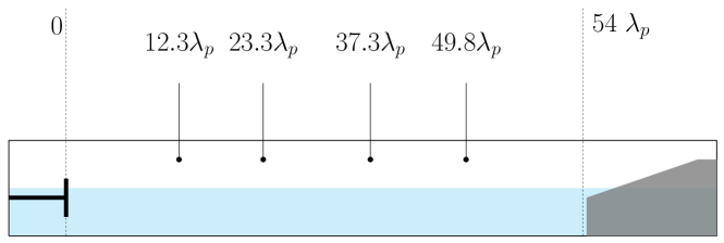
Figure 1. Sketch of laboratory experiments in the wave tank. The wave maker is placed on the left, the damping beach on the right and the four ultrasonic probes marked by their distances from the wavemaker in terms of the peak wavelength $\lambda_{p}$.

The experiments were performed in a wave flume at the Department of Mathematics at the University of Oslo. The dimensions of the tank and the setup are sketched in Figure 1. The wave tank is 24.6 m long, 0.5 m wide and was filled to a mean water depth $h=0.7$ m.

Unidirectional waves were mechanically generated at one end of the tank by a hydraulic piston, programmed according to a Torsethaugen spectrum with characteristics described below.

A 3 m long beach at the opposite end of the tank damped the waves to prevent reflection. The surface elevation was measured with four ultrasonic probes at the positions indicated in Figure 1. Key parameters for the laboratory experiment are listed in Tab. 1. Visual inspection during the experiments did not reveal wave breaking, although the measurements do indicate dissipation.

Table 1. Key parameters for laboratory experiments and simulations.

	Laboratory	Simulation
Number of probes/points along the tank	4	1024
Total time [$T_{p}$]	3058	277
Start time for analysis [$T_{p}$]	117	119
Analysis time [$T_{p}$]	2822	158
Number of simulations	1	54

The Torsethaugen spectrum applied herein is given in its simplified version for windsea dominated spectra (Veritas, 2014),

(1) $$\begin{split}&S(f)=\sum_{j=W,S}\frac{1}{16}H_{s_{j}}^{2}T_{p_{j}}S_{n_{j}}(f_{n_{j}})\\ &S_{n_{j}}=3.26A_{\nu_{j}}\Gamma_{s_{j}}\nu_{j}\\ &A_{\nu_{W}}=\left[1+1.1\left(\ln(\nu)\right)^{1.19}\right]/\nu\\ &A_{\nu_{S}}=1\\ &\Gamma_{s_{j}}=f_{n_{j}}^{-4}\exp\left[-f_{n_{j}}^{-4}\right]\\ &f_{n_{j}}=fT_{p_{j}}\\ &\nu_{W}=\nu^{\exp\left[-\frac{1}{2\alpha^{2}}\left(f_{n_{W}}-1\right)^{2}\right]}\\ &\nu=35\left[\frac{2\pi H_{s_{W}}}{gT_{p_{W}}^{2}}\right]^{0.857}\\ &\alpha=\left\{\begin{array}[]{cc}0.07&f_{n_{j}}<1\\ 0.09&f_{n_{j}}\geq 1\end{array}\right.\\ &\nu_{S}=1\end{split}$$

The values for the peak period, $T_{p}$, peak frequency, $\omega_{p}$, and significant wave height, $H_{s}$, are summarized in Table 2. Parameters for windsea and swell are distinguished by the corresponding subindices $W$ and $S$. We have renamed the shape factor $\gamma$ in Veritas (2014) to $\nu$ to avoid collision with the skewness $\gamma$ to be discussed later. Similarly, we use $\alpha$ instead of $\sigma$, since the standard deviation $\sigma$ will play a role later in the document.

We believe that the peak wavelength is still long enough to suppress cross-tank modulations provoked by modulational instability, the parameter $\mu$ of Trulsen-1999-PF-11-235 having the value $\mu=0.4\gg 0.1$ for the peak period which should ensure we are outside the domain of transversal modulationally unstable modes.

3. Setup of the numerical wave tank

Numerical simulations were carried out with a higher order spectral method, the HOS-NWT numerical wave tank described by Bonnefoy et al. (2009) and Ducrozet et al. (2012). We applied a 1D wave tank with the same scale as in the laboratory, spatially discretized at 1024 points. The waterdepth was set to five meters. A numerical wave paddle at one end of the tank was programmed to generate a two-peak spectrum

(2) $$S(f)=\sum_{j={\mathrm{W,S}}}{\frac{H_{sj}^{2}T_{pj}\left(\nu_{j}+0.25\right)^{\nu_{j}}}{4\Gamma(\nu_{j})\left(T_{pj}f\right)^{(4\nu_{j}+1)}}\exp\left(-\frac{\nu_{j}+0.25}{\left(T_{p}f\right)^{4}}\right)}$$

according to Ochi and Hubble (1976). The formulation is a superpostion of the frequency spectra of windsea, indexed by $\mathrm{W}$ and a swell spectrum, marked by the index $\mathrm{S}$. Both spectra are defined by the same formula depending on the significant wave height, $H_{s_{j}}$, the peak period, $T_{p_{j}}$, the shape factor $\nu_{j}$ which was set to 3.3 for swell and windsea and the Gamma function $\Gamma$.

The Ochi & Hubble spectrum was preferred for the simulations since increasing the energy in the swell does not affect the energy content in the windsea part as much as in the Torsethaugen model. In addition, the swell was varied over a larger range in comparison to the laboratory, to capture a greater variation of cases. The performance characteristics of the paddle were set to the default values. The damping beach was simulated by the inherent numerical beach with an absorption coefficient of unity (Bonnefoy et al., 2009; Ducrozet et al., 2012).

Key parameters for the numerical simulations are listed in Tab. 1.

4. Characterization of the sea states

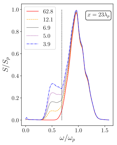
(a)

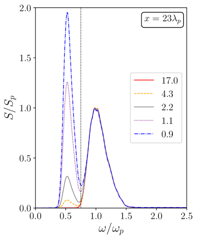
(b)

Figure 2. Scaled spectra for the different laboratory experiments and simulations. The spectra are distinguished by the Sea Swell Energy Ratio (SSER) as defined by Guedes Soares (1984).

In the simulations the spectra transform fast in the vicinity of the wavemaker but beyond five peak wavelengths from the wavemaker the spectra retain their shape approximately. Figure 2 shows an example of the spectra at the position $x=23~{}\lambda_{p}$. The vertical dotted lines mark the splitting frequencies $\omega_{m}$ that were employed to separate the combined swell and windsea ($\mathrm{SW}$) into swell ($\mathrm{S}$) and windsea ($\mathrm{W}$) contributions. Torsethaugen and Ochi & Hubble spectra require different splitting frequencies, resulting in $\omega_{m}=0.685~{}\omega_{p}$ for laboratory and $\omega_{m}=0.75~{}\omega_{p}$ for simulation. The different sea states are labeled by the sea-swell energy ratio (SSER) as suggested by Guedes Soares (1984),

(3) $$\mathrm{SSER}=\frac{m_{0\mathrm{W}}}{m_{0\mathrm{S}}},$$

based on the zeroth spectral moments for windsea, $m_{0\mathrm{W}}$, and swell $m_{0\mathrm{S}}$.

One of the key techniques employed in the analysis below is the partitioning of the two wave systems. The windsea was extracted by highpass filter (HP) and the swell by lowpass filter (LP). A similar technique was employed by e.g. Trulsen et al. (2015) and Støle-Hentschel et al. (2018).

Since the windsea spectrum is equal for all studied cases, its spectral peak $S_{p}=S_{p\mathrm{W}}$ at the frequency $\omega_{p}=\omega_{p\mathrm{W}}$ serves as scaling parameters and the indices for windsea are dropped for these two parameters.

The wave steepness and the Benjamin-Feir index (BFI) are characteristics of the sea states that can only be estimated for individual wave systems (Trulsen et al., 2015; Støle-Hentschel et al., 2018). The wave steepness definition employed here is $\varepsilon=k_{p}a_{c}$ where $a_{c}=H_{s}/\sqrt{8}$ is a characteristic amplitude and where $H_{s}$ is the significant wave height defined as four times the standard deviation of the surface elevation. We only consider the BFI of the windsea system $\mathrm{BFI}_{W}=\varepsilon_{W}\omega_{p}/\Delta_{W}$, where $\Delta_{W}$ is the ’half width at half peak’. Tab. 2 summarizes the characteristics of the wave system employed in this study.

Table 2. Wave parameters for laboratory experiments and simulations.

	Laboratory	Simulation
$T_{p_{W}}$ [s]	0.51	0.72
$\lambda_{p_{W}}$ [m]	0.40	0.80
$T_{p_{S}}$ [s]	0.97	1.37
$\lambda_{p_{S}}$ [m]	1.45	2.9
$H_{s_{W}}$ [cm]	1.2	2.3
$H_{s_{S}}$ [cm]	{0.06, 0.11, 0.17, 0.22}	{0.10,0.50,0.90,1.8}
$\omega_{m}~{}[\omega_{p}]$	0.685	0.750
$\varepsilon_{W}$ ($x=23\lambda_{p}$)	0.069	0.062
$\varepsilon_{S}$ ($x=23\lambda_{p}$)	$\leq 0.003$	$\leq 0.009$
$\mathrm{BFI}_{W}$	$\leq 0.06$	$\leq 0.25$

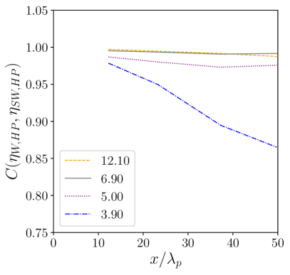
(a)

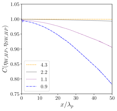
(b)

Figure 3. The correlation coefficient between highpass filtered windsea and highpass filtered mixed cases with the indicated SSER.

As a first estimate of the degree of interaction between swell and windsea we calculate the correlation coefficient of pure windsea waves and the windsea part of a combined windsea and swell sea state,

(4) $$C(\eta_{\mathrm{W,HP}},\eta_{\mathrm{SW,HP}})=\frac{\mathrm{Cov}(\eta_{\mathrm{W,HP}},\eta_{\mathrm{SW,HP}})}{\sigma_{\mathrm{W,HP}}\sigma_{\mathrm{SW,HP}}}=\frac{E[\eta_{\mathrm{W,HP}}\eta_{\mathrm{SW,HP}}]}{\sigma_{\mathrm{W,HP}}\sigma_{\mathrm{SW,HP}}},$$

where $\eta_{\mathrm{W,HP}}$ and $\eta_{\mathrm{SW,HP}}$ are the surface elevations of pure windsea and combined swell and windsea both filtered by a high pass filter. The corresponding standard deviations are denoted $\sigma_{\mathrm{W,HP}}$ and $\sigma_{\mathrm{SW,HP}}$. In the case of the simulations, the correlation coefficient shown in Figure 3b was averaged over all simulations. Close to the wavemaker, the pure windsea and the windsea parts of the mixed seas are practically identical for all cases. In the development along the tank the correlation coefficient decays depending on the strength of the swell. Close to the damping beach, the correlation coefficient decays to a level of 0.85 for the laboratory and 0.75 for the simulation for the strongest swell. These observations suggest that the swell has only marginal influence on the phases of the windsea waves over the given evolution length.

5. Kurtosis and skewness for different sea states

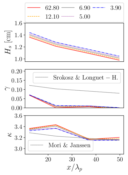
(a)

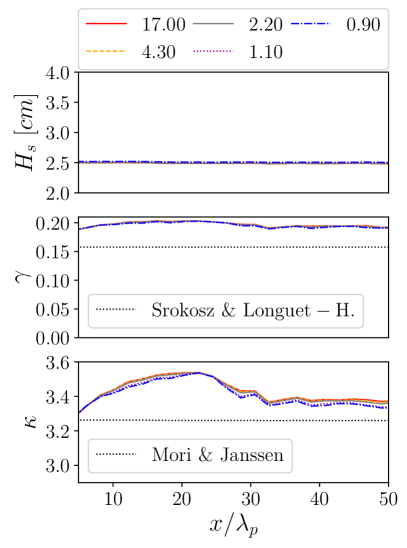
(b)

Figure 4. Significant wave height, skewness and kurtosos for the highpass filtered waves, labeled by the SSER coefficient. With a confidence of 80%, the deviation from the mean is [-0.07, 0.02] for skewness and [-0.1,0.4] for kurtosis in the laboratory. The corresponding intervals for the simulations are [-0.1,0.2] and [-0.5,0.9]. For comparison we added theoretical results by Srokosz and Longuet-Higgins (1986); Mori and Janssen (2006) for longcrested waves of narrow bandwidth.

Figure 4 presents the laboratory measurements and the simulation results in terms of $H_{s}$, skewness and kurtosis for the highpass filtered windsea waves. In the case of the laboratory, the local skewness, $\gamma$, and the local kurtosis, $\kappa$, were computed for each fixed position along the tank. The damping beach in the laboratory is too short for the longest waves leading to seiche modes. These have been filtered by a high pass filtered for the entire data analysis. For the simulations, we have employed a lower time resolution of $\Delta t=0.14$ s and the part of the simulation time subject to analysis is limited to 77 $T_{p}$. To ensure sufficient surface elevation measurements for adequate estimates or kurtosis and skewness, 32 neighboring grid points were considered as one evaluation point in space, and 10 simulations were merged; thus, the mean values and the confidence intervals are based on 50 simulations arranged into five groups. The strong decay of $H_{s}$ in the laboratory is attributed to dissipation that has a strong effect on the experiment due to the short peak wavelength of the windsea spectrum. This reduction in wave steepness affects the kurtosis and the skewness, as reflected in the reference curves based on Srokosz and Longuet-Higgins (1986) and Mori and Janssen (2006). For the simulations, the significant wave height is constant along the tank. Overall, the difference in skewness and kurtosis for the different spectra is smaller than the variation of the values.

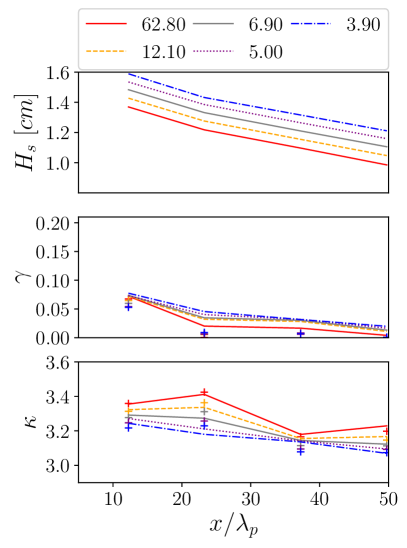
(a)

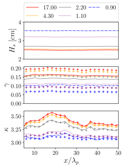
(b)

Figure 5. Significant wave height, skewness and kurtosis for the combined windsea and swell wave field (lines). Estimates based on Eq. 5 and 6 are marked by ’+’ with the same colors as the corresponding full sea states. With a confidence of 80%, the deviation from the mean is [-0.007, 0.05] for skewness and [-0.06,0.4] for kurtosis. The corresponding intervals for the simulations are [-0.02,0.06] and [-0.09,0.32].

We also analyze the local skewness and the local kurtosis for the waves of the entire spectra (Figure 5). Both the laboratory and the simulation results show that the SSER is correlated to the kurtosis of combined seas. The same is shown for the skewness in the simulations. In the laboratory, the skewness behaves differently, however the variation between the cases is small.

From the definition of skewness and kurtosis, we calculate reference values for skewness and kurtosis of combined sea states based on the assumption that the two systems are independent. From the analysis of the correlation coefficient, we anticipate that this may be a good approximation. We find the formulas

(5) $$\gamma_{\mathrm{SW}}=\frac{\gamma_{\mathrm{S}}\sigma_{\mathrm{S}}^{3}+\gamma_{\mathrm{W}}\sigma_{\mathrm{W}}^{3}}{(\sigma_{\mathrm{S}}^{2}+\sigma_{\mathrm{W}}^{2})^{3/2}}$$

and

(6) $$\kappa_{\mathrm{SW}}=\frac{\kappa_{\mathrm{S}}\sigma_{\mathrm{S}}^{4}+6\sigma_{\mathrm{S}}^{2}\sigma_{\mathrm{W}}^{2}+\kappa_{\mathrm{W}}\sigma_{\mathrm{W}}^{4}}{(\sigma_{\mathrm{S}}^{2}+\sigma_{\mathrm{W}}^{2})^{2}}$$

with $\{\sigma_{\mathrm{S}}^{2},\gamma_{\mathrm{S}},\kappa_{\mathrm{S}}\}$ the variance, skewness and kurtosis of the swell partition, and $\{\sigma_{\mathrm{W}}^{2},\gamma_{\mathrm{W}},\kappa_{\mathrm{W}}\}$ the variance, skewness and kurtosis of the windsea partition. Figure 5 shows that the analysis of the entire wave system differs clearly from the analysis of the windsea system (Figure 4). The estimates in Eq. 5 and 6 are similar but not equal to the calculated values.

The kurtosis of the windsea waves is generally high in the presented analysis which is expected for longcrested waves. According to Gramstad and Trulsen (2007), wave crests longer than ten times the wavelength are associated with very high kurtosis values, even for large spectral bandwidths that are not typically associated with modulational instability according to a low Benjamin-Feir index (Janssen, 2003).

6. Exceedance probability of wave envelope

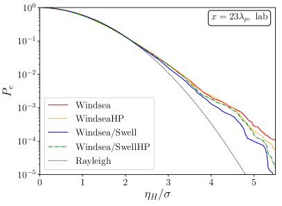
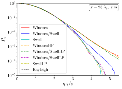
Figure 6. Exceedance probability of Hilbert envelopes scaled by the standard deviation of the underlying surface elevation at one position. The mixed sea is based on the maximum swell for laboratory (SSER=3.9) and simulation (SSER=0.9), respectively. The windsea has a SSER of 62.8 for the laboratory and 17.0 for the simulation.

We study the exceedance probability of the Hilbert envelope to retrieve insight in the amount of extreme events in the different cases. The Hilbert wave envelope was computed according to

(7) $$\eta_{H}=\sqrt{\eta^{2}+\tilde{\eta}^{2}}$$

where $\tilde{\eta}$ is the Hilbert transform of the surface elevation $\eta$. The envelopes were scaled by the standard deviation of the corresponding surface elevation. For reference, we compare the probability distributions of the different cases with the Rayleigh distribution, which is the distribution of the Hilbert envelope of a Gaussian process.

In the presentation of the exceedance curves in this and the next chapter, we focus on pure windsea and the mixed sea with the strongest swell for laboratory and simulation. Pure swell simulations were added for comparison. The different sea states are analysed both filtered and unfiltered. The results in Figure 6 are clearer for the simulations than for the laboratory experiments. The swell envelopes of all configurations coincide with the Rayleigh distribution in good correspondence with the fact that the swell is essentially linear. While the envelopes of the complete wave fields differ, their windsea contributions are similar and deviate clearly from Gaussian behavior.

7. Exceedance probability of crest height

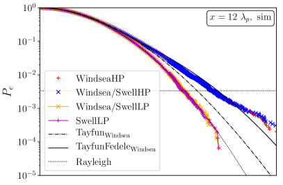
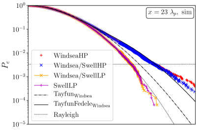
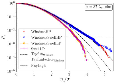
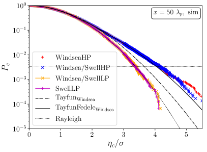
Figure 7. Exceedance probability of crest heights scaled by the standard deviation of the corresponding surface elevation at four positions along the numerical wave tank. SSER values are 17 and 0.9 for windsea and mixed seas respectively.

Finally, we investigate the exceedance probability of the crest height, $\eta_{c}$ scaled by the standard deviation, $\sigma$ of the corresponding surface elevation (see Figure 7). We only consider the exceedance probability of the crests for the simulations since the number of measured crests in the laboratory was too small for meaningful analysis. For better results on extreme cases, the number of simulations was increased to 180, compared to that of Tab. 1. The simulated data was interpolated by truncated Fourier series expansion in time before determining the crest height as maximum between two zero crossings. Below the horizontal dotted lines the number of crests is lower than one hundred which is considered too few for statistical significance.

The exceedance probability is characterized by local variation, similar to what we previously found for the skewness and the kurtosis. To illustrate the amount of local variation, we show the exceedance probability at four locations along the numerical wavetank (see Figure 7).

When comparing the waves after partitioning into swell and windsea, the statistics are approximately identical irrespective if the other wave system is present or not.

As reference distributions, we consider Rayleigh, Tayfun (Tayfun, 1980) and Tayfun-Fedele (Fedele et al., 2016; Tayfun and Fedele, 2007). The wave crests of narrow banded linear waves are Rayleigh distributed. Although the simulated swell is not particularly narrow-banded, its crests are found to be Rayleigh distributed. The Tayfun distribution, here calculated based on the standard deviation of the windsea waves, is the reference distribution for narrow banded second order wave crests. The windsea distributions clearly exceed Tayfun even though they are clearly not narrow-banded. Hence we anticipate that nonlinearities of third order must play an important role for the windsea waves. As an approximation to a third order distribution of crest heights we employ the Tayfun-Fedele distribution. It is a continuation of the second-order Tayfun distribution by the Gram-Charlier series up to the fourth cumulant (Fedele et al., 2016; Tayfun and Fedele, 2007). The distribution changes its form with the wave steepness by its dependence on the skewness and the occurrence of extreme values by the incorporation of the kurtosis. The Tayfun-Fedele distribution shows good agreement with the simulated windsea exceedance probability of crest heights.

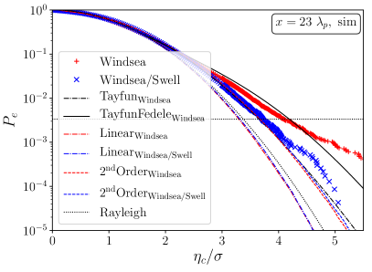
Figure 8. Exceedance probabilities of crest heights of unfiltered sea states. SSER values are 17 and 0.9 for windsea and mixed seas respectively.

Figure 8 reveals that the combined swell and windsea results in an exceedance probability for crest heights between that of pure swell and that of pure windsea that is coincidentally similar to that of narrow-banded waves of second order. Simulations of linear theory and second order theory (Forristall, 2000) were added.

8. Discussion

Our results show that combined sea states require a different analysis than single wave systems. A unified steepness cannot be defined for the combination of multiple wave systems (Naciri and Mei, 1992, 1993; Gramstad and Trulsen, 2010, 2011; Støle-Hentschel et al., 2018; Trulsen et al., 2015). We have shown that the partitioning of the spectrum is not only necessary for estimating the various partial steepnesses, but also for better understanding of the statistics of extreme waves.

We observe that the results are more distinct for the simulations than for the laboratory, which we attribute mainly to the different spectra that were applied. The windsea parts of the Torsethaugen spectra differ considerably for minor changes of the swell part, while the windsea part of Ochi & Hubble spectra are very similar, even for very different swell contributions.

As formulated in Eq. 5 and 6, skewness and kurtosis for mixed sea are weighted combinations of skewness and kurtosis of the separated systems. Therefore, the combination of a Gaussian and a strongly non-Gaussian system of equivalent $H_{s}$ will appear weakly non-Gaussian. A similar behavior seems to occur for the exceedance probabilities. In our study, the swell affects the windsea so little that the two systems may be regarded as independent. In this case we believe that extreme wave statistics for the combined sea may underestimate how dangerous the combined sea state really is.

9. Conclusion

We have shown that extreme wave statistics of windsea can be nearly unaffected by the presence of a following swell. However, this only becomes apparent if the two sea states are analysed separately. Analysis of the entire wave system as a whole gives the impression that the mixed sea has milder extreme wave statistics than the pure windsea, especially when the nonlinearity in the two systems clearly differs. Therefore we believe that mixed sea states should be partitioned, and analysis be performed on each partition, in order to fully comprehend the combined extreme wave statistics.

References

- Bonnefoy et al. (2009) Bonnefoy, F., Ducrozet, G., Le Touzé, D., and Ferrant, P. (2009). Time-domain simulation of nonlinear water waves using spectral methods. Advances in Numerical Simulation of Nonlinear Water Waves.
- Boukhanovsky and Guedes Soares (2009) Boukhanovsky, A. V. and Guedes Soares, C. (2009). Modelling of multipeaked directional wave spectra. Appl. Ocean Res., 31:132–141.
- Cavaleri et al. (2012) Cavaleri, L., Bertotti, L., Torrisi, L., Bitner-Gregersen, E., Serio, M., and Onorato, M. (2012). Rogue waves in crossing seas: The Louis Majesty accident. J. Geophys. Res., 117:C00J10.
- Craik (1988) Craik, A. D. D. (1988). Interaction of a short-wave field with a dominant long wave in deep water: Derivation from Zakharov’s spectral formulation. J. Austral. Math. Soc. B, 29:430–439.
- Ducrozet et al. (2012) Ducrozet, G., Bonnefoy, F., Le Touzé, D., and Ferrant, P. (2012). A modified High-Order Spectral method for wavemaker modeling in a numerical wave tank. Eur. J. Mech. B/Fluids, 34:19–34.
- Fedele et al. (2016) Fedele, F., Brennan, J., Ponce de León, S., Dudley, J., and Dias, F. (2016). Real world ocean rogue waves explained without the modulational instability. Scientific Reports, 6:27715.
- Forristall (2000) Forristall, G. Z. (2000). Wave crest distributions: observations and second-order theory. J. Phys. Oceanogr., 30:1931–1943.
- Gramstad and Trulsen (2007) Gramstad, O. and Trulsen, K. (2007). Influence of crest and group length on the occurrence of freak waves. J. Fluid Mech., 582:463–472.
- Gramstad and Trulsen (2010) Gramstad, O. and Trulsen, K. (2010). Can swell increase the number of freak waves in a wind-sea? J. Fluid Mech., 650:57–79.
- Gramstad and Trulsen (2011) Gramstad, O. and Trulsen, K. (2011). Fourth-order coupled nonlinear Schrödinger equations for gravity waves on deep water. Phys. Fluids, 23:062102.
- Grimshaw (1988) Grimshaw, R. (1988). The modulation of short gravity waves by long waves or currents. J. Austral. Math. Soc. B, 29:410–429.
- Guedes Soares (1984) Guedes Soares, C. (1984). Representation of double-peaked sea wave spectra. Ocean Engineering, 11:185–207.
- Guedes Soares (1991) Guedes Soares, C. (1991). On the occurrence of double peaked wave spectra. Ocean Engineering, 18:167–171.
- Henyey et al. (1988) Henyey, F. S., Creamer, D. B., Dysthe, K. B., Schult, R. L., and Wright, J. A. (1988). The energy and action of small waves riding on large waves. J. Fluid Mech., 189:443–462.
- Janssen (2003) Janssen, P. A. E. M. (2003). Nonlinear four-wave interactions and freak waves. J. Phys. Oceanogr., 33:863–884.
- Longuet-Higgins (1987) Longuet-Higgins, M. S. (1987). The propagation of short surface waves on longer gravity waves. J. Fluid Mech., 177:293–306.
- Longuet-Higgins and Stewart (1960) Longuet-Higgins, M. S. and Stewart, R. W. (1960). Changes in the form of short gravity waves on long waves and tidal currents. J. Fluid Mech., 8:565–583.
- Masson (1993) Masson, D. (1993). On the nonlinear coupling between swell and wind waves. J. Phys. Oceanogr., 23:1249–1258.
- Mori and Janssen (2006) Mori, N. and Janssen, P. A. E. M. (2006). On kurtosis and occurrence probability of freak waves. J. Phys. Oceanogr., 36:1471–1483.
- Naciri and Mei (1992) Naciri, M. and Mei, C. C. (1992). Evolution of a short surface wave on a very long surface wave of finite amplitude. J. Fluid Mech., 235:415–452.
- Naciri and Mei (1993) Naciri, M. and Mei, C. C. (1993). Evolution of short gravity waves on long gravity waves. Phys. Fluids A, 5:1869–1878.
- Naciri and Mei (1994) Naciri, M. and Mei, C. C. (1994). Two-dimensional modulation and instability of a short wave riding on a finite-amplitude long wave. Wave Motion, 20:211–232.
- Ochi and Hubble (1976) Ochi, M. K. and Hubble, E. N. (1976). Six-parameter wave spectra. In Proc 15th Coastal Engineeringe Conference, pages 301–328.
- Onorato et al. (2006) Onorato, M., Osborne, A. R., and Serio, M. (2006). Modulational instability in crossing sea states: A possible mechanism for the formation of freak waves. Phys. Rev. Lett., 96:014503.
- Petrova and Guedes Soares (2014) Petrova, P. and Guedes Soares, C. (2014). Distributions of nonlinear wave amplitudes and heights from laboratory generated following and crossing bimodal seas. Natural Hazards and Earth System Sciences, 14(5):1207–1222.
- Petrova and Guedes Soares (2009) Petrova, P. G. and Guedes Soares, C. (2009). Probability distributions of wave heights in bimodal seas in an offshore basin. Applied Ocean Research, 31(2):90–100.
- Petrova and Guedes Soares (2011) Petrova, P. G. and Guedes Soares, C. (2011). Wave height distributions in bimodal sea states from offshore basins. Ocean Engineering, 38(4):658–672.
- Regev et al. (2008) Regev, A., Agnon, Y., Stiassnie, M., and Gramstad, O. (2008). Sea–swell interaction as a mechanism for the generation of freak waves. Phys. Fluids, 20:112102.
- Srokosz and Longuet-Higgins (1986) Srokosz, M. A. and Longuet-Higgins, M. S. (1986). On the skewness of sea-surface elevation. J. Fluid Mech., 164:487–497.
- Støle-Hentschel et al. (2018) Støle-Hentschel, S., Trulsen, K., Rye, L. B., and Raustøl, A. (2018). Extreme wave statistics of counter-propagating, irregular, long-crested sea states. Phys. Fluids, 30:067102.
- Tamura et al. (2009) Tamura, H., Waseda, T., and Miyazawa, Y. (2009). Freakish sea state and swell–windsea coupling: Numerical study of the Suwa–Maru incident. Geophys. Res. Lett., 36:L01607.
- Tayfun (1980) Tayfun, M. A. (1980). Narrow-band nonlinear sea waves. J. Geophys. Res., 85:1548–1552.
- Tayfun and Fedele (2007) Tayfun, M. A. and Fedele, F. (2007). Wave-height distributions and nonlinear effects. Ocean Engineering, 34:1631–1649.
- Toffoli et al. (2011) Toffoli, A., Bitner-Gregersen, E. M., Osborne, A. R., Serio, M., Monbaliu, J., and Onorato, M. (2011). Extreme waves in random crossing seas: Laboratory experiments and numerical simulations. Geophys. Res. Lett., 38:L06605.
- Toffoli et al. (2005) Toffoli, A., Lefevre, J. M., Bitner-Gregersen, E., and Monbaliu, J. (2005). Towards the identification of warning criteria: Analysis of a ship accident database. Appl. Ocean Res., 27:281–291.
- Trulsen et al. (2015) Trulsen, K., Nieto Borge, J. C., Gramstad, O., Aouf, L., and Lefèvre, J.-M. (2015). Crossing sea state and rogue wave probability during the Prestige accident. J. Geophys. Res. Oceans, 120:7113–7136.
- Veritas (2014) Veritas, D. N. (2014). Recommended practice for environmental conditions and environmental loads (dnv-rp-c205). Hovik, Norway.
- Waseda et al. (2014) Waseda, T., In, K., Kiyomatsu, K., Tamura, H., Miyazawa, Y., and Iyama, K. (2014). Predicting freakish sea state with an operational third-generation wave model. Nat. Hazards Earth Syst. Sci., 14:945–957.
- Waseda et al. (2012) Waseda, T., Tamura, H., and Kinoshita, T. (2012). Freakish sea index and sea states during ship accidents. J. Mar. Sci. Technol., 17:305–314.
- Zhang and Melville (1990) Zhang, J. and Melville, W. K. (1990). Evolution of weakly nonlinear short waves riding on long gravity waves. J. Fluid Mech., 214:321–346.
- Zhang and Melville (1992) Zhang, J. and Melville, W. K. (1992). On the stability of weakly nonlinear short waves on finite-amplitude long gravity waves. J. Fluid Mech., 243:51–72.