Abstract

We study two-interval holographic entanglement entropy and entanglement wedge cross section in cutoff AdS. In particular, we investigate phase transitions of them. For two-interval entanglement entropy, the transition point monotonically decreases with a deformation parameter, which means that by the $T\bar{T}$ deformation the degrees of freedom in subsystems are decreasing. This implies that the effect of the $T\bar{T}$ deformation can be regarded as the rescaling of the energy scale. We also study entanglement wedge cross section in cutoff AdS, and our result implies that for the entanglement of purification in the $T\bar{T}$ deformed CFTs phase transition could occur even for fixed subsystems.

1 Introduction

The AdS/CFT correspondence [1, 2, 3] is a very powerful statement, which has been utilized to explore nonperturbative aspects of quantum field theories for ages. In field theory side of the AdS/CFT, conformal field theory is by definition a UV complete framework, in which at all energy scales a local quantum field theory does exist. This remains true for relevant or marginal deformations of CFTs which preserve the existence of a UV fixed point. Then, a natural question arises: can the AdS/CFT be extended to a correspondence between nearly AdS and nearly CFT with an irrelevant deformations of CFTs? In the context of AdS₃/CFT₂ correspondence, McGough, Mezei, and Verlinde have recently proposed an intriguing extension of the AdS/CFT [4], which is based on so called an integrable $T\bar{T}$ deformation of CFT [5, 6]. On the bulk side, the boundary lies not at asymptotic infinity, but instead is located at a finite radial position. The dual quantum field theory is no longer conformal, but is described by a QFT deformed by the remarkable $T\bar{T}$ operator of Zamolodchikov [7]. This deformed integrable quantum field theory can be regarded as an efective field theory with a finite UV cutoff. The bulk side of this proposed duality has an interesting viewpoint: the AdS/CFT with a finite boundary. Moving the boundary inward could shed light on the question of the emergence of bulk locality. In particular, [8, 9] show that such cutoffs are dual to some deformation of the orginal CFT.

The $T\bar{T}$ deformation of two dimensional CFTs provides an exactly solvable model of quantum field theory with an UV cutoff [5, 6]. Any CFT can be deformed by this operator, defining a one-parameter family of theories labelled by a dimensionful deformation parameter $\mu$. Here we take $\mu$ to be positive, and the deformation is written as

$$S_{\text{QFT}}=S_{\text{CFT}}+\mu\int d^{2}x\,T\bar{T},$$ (1.1)

where $T\bar{T}$ denotes the composite irrelevant operator given by the product of the left- and right-moving components of the stress tensor [7]. By finite $\mu$ we mean that there is a one parameter family of theories defined by $dS^{(\mu)}_{\text{QFT}}/d\mu=\int d^{2}x(T\bar{T})_{\mu}$, where the $(T\bar{T})_{\mu}$ emphasizes that in this equation we have to use the stress tensor defined through $S^{(\mu)}_{\text{QFT}}$. The system is exactly solvable under this deformation (1.1), in the sense that the deformed theory also possesses an infinite set of conserved charges and allows one to exactly compute interesting physical quantities.

On the flip side, the $T\bar{T}$ deformation opens a new window to study the AdS/CFT correspondence itself. It is a double-trace deformation, and could change the boundary condition of the AdS gravity. For a $T\bar{T}$ deformed holographic CFT, a deformed AdS/CFT has been proposed, in which the dual AdS₃ gravity should be defined in a finite region, with the asymptotic boundary being at a finite radial position [4]. More precisely if a CFT has a gravity dual, then the deformed theory is dual to the original gravitational theory with the new boundary at $r=r_{c}$. The relation between the deformation parameter $\mu$ and the finite radial position $r_{c}$ is given by

$$\mu=\frac{16\pi G_{N}}{r_{c}^{2}}=\frac{24\pi}{c}\frac{1}{r_{c}^{2}},$$ (1.2)

where we set the AdS radius to be $1$, and c is the central charge of the original CFT. This new correspondence has been checked from various points of view, and more on the holographic interpretation of the $T\bar{T}$ deformation has also been studied, see e.g. [10, 11, 12, 13, 14, 15, 16, 17].

In a holographic CFT, the entanglement entropy could be captured by the area of the minimal surface extended into the dual AdS bulk geometry via the Ryu-Takayanagi formula [18], and entanglement entropy in general can extract a large amount of quantum feature for strongly interacting systems. As we have seen, according to [4] in the gravity side the $T\bar{T}$ deformed geometry is a cutoff AdS. Thus, the holographic entanglement entropy may be directly affected by the deformation, and in fact it is found that entanglement entropies in the $T\bar{T}$ deformed CFTs generically have corrections due to the deformation, see e.g. [19, 20, 21]. In this paper, we focus on the two-interval holographic entanglement entropy [22, 23, 24, 25] and the holographic entanglement of purification [26] in cutoff AdS. By considering the new duality proposed in [4], assuming that the RT formula still holds, we study the holographic entanglements in the $T\bar{T}$ deformed CFTs. In particular, we consider phase transitions of holographic entanglements in the cutoff AdS and investigate its implication in the AdS/CFT correspondence. It turns out that our results imply subsystems are effectively getting small by the $T\bar{T}$ deformation, in other words we can interpret them as the degrees of freedom in the subsystems are decreasing. Our results are consistent with [27], in which the entanglement entropy in a boosted system is computed and the Lorentz contracted subsystem could be regarded as a $T\bar{T}$ deformed system. Also for entanlement of purification, in the $T\bar{T}$ deformed CFTs the phase transition could occur for fixed subsystems.

The rest of the paper is organized as follows. In Sec. 2, we consider two-interval holographic entanglement entropy and its phase transition. In the cutoff AdS, we will find that the transition point is monotonically decreasing, which means that the subsystem in the boundary is effectively getting small. In Sec. 3, we also investigate the effect of the $T\bar{T}$ deformation on the entanglement wedge cross section, which is conjectured to be a gravity dual of the entanglement of purification in holographic CFTs [26]. In Sec. 4, we give a conclusion and some discussions.

2 Two-interval entanglement entropy

In this section we discuss two-interval holographic entanglement entropy and its transition in cutoff AdS. For this purpose, we need to compute the lengths of geodesics in cutoff AdS and to compare them. By numerically solving the transition point, we will find it is monotonically decreasing with the deformation. In the field theory side, this result can be interpreted in a way that the degrees of freedom of the subsystems are decreasing.

2.1 Geodesic in cutoff AdS

For later use, let us begin with the computation of a geodesic in $\mathrm{AdS_{3}}$. Pure $\mathrm{AdS_{3}}$ metric in Poincar$\acute{\mathrm{e}}$ coordinate is

$$ds^{2}=\frac{-dt^{2}+dx^{2}+dz^{2}}{z^{2}},$$ (2.1)

where the AdS radius is set to $1$. For a static curve in $\mathrm{AdS_{3}}$ at a canonical time slice, the induced metric on it is given by

$$ds_{static}^{2} =\frac{1}{z(x)^{2}}(dx^{2}+z^{\prime}(x)^{2}dx^{2})$$

$$=\frac{1+z^{\prime}(x)^{2}}{z(x)^{2}}dx^{2},$$ (2.2)

we are employing the static gauge. Euler-Lagrange equation for the length functional of the curve

$$L[z]=\int\frac{\sqrt{1+z^{\prime}(x)^{2}}}{z(x)}dx$$ (2.3)

yields the equation of motion for $z(x)$. Solving it with boundary condition

$$z^{\prime}(0)=0$$ (2.4)

and

$$z(0)=0\;\mathrm{or}\;z(a)=0$$ (2.5)

gives us semi-circle solutions with the radius $a$.

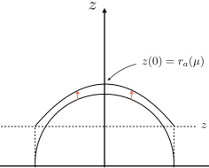
Figure 1: A deformed geodesic in the $T\bar{T}$ deformed geometry.

Let us move on to the $T\bar{T}$ deformed geometry, namely cutoff AdS. We introduce a finite radial cutoff [4]

$$r_{c}^{2}=\frac{24\pi}{\mu c}.$$ (2.6)

In $z$ coordinate, the radial cutoff is located at

$$z_{c}=\frac{1}{r_{c}}=\sqrt{\frac{\mu c}{24\pi}}.$$ (2.7)

We now have $\mathrm{AdS_{3}}$ spacetime with Dirichlet boundary surface at $z=z_{c}$ :

$$ds^{2}=\frac{-dt^{2}+dx^{2}+dz^{2}}{z^{2}},\;z_{c}\leq z\leq\infty.$$ (2.8)

Then, the length functional yields the same equation of motion as before but we need to impose a boundary condition so that

$$z^{\prime}(0)=0$$ (2.9)

and

$$z(a)=\sqrt{\frac{\mu c}{24\pi}}=z_{c}.$$ (2.10)

A solution is given by

$$z(x)=\left(a^{2}+z_{c}^{2}-x^{2}\right)^{1/2},\;-a\leq x\leq a.$$ (2.11)

This solution is schematically drawn in Fig. 1, where we write the deformed radius as

$$z(0)=\left(a^{2}+z_{c}^{2}\right)^{1/2}=:r_{a}(\mu).$$ (2.12)

In this kind of deformed geometry, the corrections of holographic entanglement entropy are calculated and they seem to be consistent with those of the deformed CFT [19, 20].

2.2 Two-interval entanglement entropy in cutoff AdS

Let us now consider two-interval entanglement entropy and its transition. For simplicity, we just focus on symmetric configurations shown in Figs. 2 ($a$), ($b$). We have two choices to obtain the geodesics which end on the endpoints of subsystems $A$ and $B$. So, when one considers two-interval subsystems like this configuration, the holographic entanglement entropy is given by [24, 25]

$$S_{AB}=\frac{1}{4G_{N}}\min\{\lambda_{a}+\lambda_{b},~{}2\lambda_{ab}\},$$ (2.13)

where $\lambda_{a},\,\lambda_{b},\,\lambda_{ab}$ are the length of $\gamma_{a},\,\gamma_{b},\,\gamma_{ab}$, respectively. The configuration that gives the entropy is the one in which the geodesics have minimal total length, and generically the phase transition between the two occurs. To see the transition, we compute the length of the geodesics in Fig. 2 ($a$) and Fig. 2 ($b$), and compare $\lambda_{a}+\lambda_{b}$ and $2\lambda_{ab}$. When $\lambda_{a}+\lambda_{b}\leq 2\lambda_{ab}$, the configuration in Fig. 2 ($a$) is realized, while when $\lambda_{a}+\lambda_{b}\geq 2\lambda_{ab}$, Fig. 2 ($b$) is. So let us directly calculate the lengths and compare them.

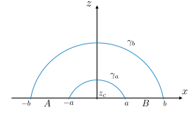
$(a)$

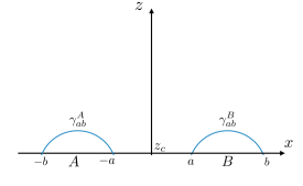
$(b)$

Figure 2: Two configurations of geodesics for two-interval holographic entanglement entropy.

Firstly we consider the Fig. 2 ($a$) case. The geodesic $\gamma_{a}$ is, as we obtained before, given by Eq. (2.11)

$$z(x)=\left(a^{2}+z_{c}^{2}-x^{2}\right)^{1/2},\;-a\leq x\leq a.$$ (2.14)

To compute its length in the cutoff AdS, we would like to introduce a polar coordinate:

$$x =\alpha\cos\theta,$$ (2.15)

$$z =\alpha\sin\theta,$$ (2.16)

where we defined $\alpha^{2}=a^{2}+z_{c}^{2}$. Then, the induced metric on the geodesic is

$$ds^{2} =\frac{\alpha^{2}}{z^{2}}d\theta^{2}$$

$$=\frac{1}{\sin^{2}\theta}d\theta^{2}.$$ (2.17)

Using this, the length of the geodesic $\lambda_{a}$ is easily computed by

$$\lambda_{a}=\int ds=2\int_{\theta_{a}}^{\pi/2}\frac{d\theta}{\sin\theta},$$ (2.18)

where $\theta_{a}$ is defined by the relations $\cos\theta_{a}=a/\alpha,\,\sin\theta_{a}=z_{c}/\alpha$. We can integrate the above and find that

$$\lambda_{a} =\log\left(\frac{\alpha+a}{\alpha-a}\right)$$

$$=\log\left(\frac{\sqrt{1+z_{c}^{2}/a^{2}}+1}{\sqrt{1+z_{c}^{2}/a^{2}}-1}\right).$$ (2.19)

For $\lambda_{b}$, the calculation is exactly the same, so we obtain

$$\lambda_{a}+\lambda_{b}=\log\left(\frac{\sqrt{1+z_{c}^{2}/a^{2}}+1}{\sqrt{1+z_{c}^{2}/a^{2}}-1}\right)+\log\left(\frac{\sqrt{1+z_{c}^{2}/b^{2}}+1}{\sqrt{1+z_{c}^{2}/b^{2}}-1}\right).$$ (2.20)

For Fig. 2 ($b$) case, $2\lambda_{ab}$ can be also easily calculated using this results. In the $T\bar{T}$ deformed geometry, the solution of the geodesic $\gamma_{ab}^{B}$ is given by

$$z(x)=\sqrt{\left(\frac{b-a}{2}\right)^{2}+z_{c}^{2}-\left(x-\frac{a+b}{2}\right)^{2}}.$$ (2.21)

So we can conclude that

$$2\lambda_{ab} =2\lambda_{a}|_{a\rightarrow(b-a)/2}$$

$$=2\log\left(\frac{\sqrt{1+z_{c}^{2}/\left(\frac{b-a}{2}\right)^{2}}+1}{\sqrt{1+z_{c}^{2}/\left(\frac{b-a}{2}\right)^{2}}-1}\right).$$ (2.22)

2.3 Transition between the two cases

As we have seen, the holographic entanglement entropy of the two intervals is given by $\lambda_{a}+\lambda_{b}$ or $2\lambda_{ab}$ in the way that

$$S_{AB}=\frac{c}{6}\min\left\{\lambda_{a}+\lambda_{b},\;2\lambda_{ab}\right\},$$ (2.23)

where we have used the relation $c=3/2G_{N}$ [28]. Which case is smaller is determined by the difference $b-a$, or in other words the ratio $a/b$. We fix $b$ and change $a$ from $0$ to $b$ to find the transition, i.e. by solving $\lambda_{a}+\lambda_{b}=2\lambda_{ab}$ with respect to $a$, we find the transition point. When $\mu c\rightarrow 0$, $\lambda_{a}+\lambda_{b}=2\lambda_{ab}$ becomes

$$2a\times 2b=(b-a)^{2},$$ (2.24)

so when we change $a$, the transition occurs at

$$a_{0}=(3\pm 2\sqrt{2})b.$$ (2.25)

Since we are considering $a\in[0,b]$, the solution should be $a_{0}=(3-2\sqrt{2})b.$

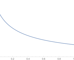
Figure 3: The transition point. In this plot we set $b=1$.

Now, let us consider entanglement entropies with finite $\mu c$. The equation we need to solve is

$$\left(\frac{\sqrt{1+z_{c}^{2}/\left(\frac{b-a}{2}\right)^{2}}+1}{\sqrt{1+z_{c}^{2}/\left(\frac{b-a}{2}\right)^{2}}-1}\right)^{2}=\frac{\sqrt{1+z_{c}^{2}/a^{2}}+1}{\sqrt{1+z_{c}^{2}/a^{2}}-1}\frac{\sqrt{1+z_{c}^{2}/b^{2}}+1}{\sqrt{1+z_{c}^{2}/b^{2}}-1},$$ (2.26)

This can be rewritten as

$$\left(\frac{b-a}{2}\right)^{2}\left(\sqrt{1+z_{c}^{2}\left(\frac{b-a}{2}\right)^{-2}}+1\right)^{2}=ab\left(\sqrt{1+\frac{z_{c}^{2}}{a^{2}}}+1\right)\left(\sqrt{1+\frac{z_{c}^{2}}{b^{2}}}+1\right).$$ (2.27)

We can see an asymptotic form of the solution to Eq. (2.27) in the small $z_{c}$ region. When $z_{c}/a,\,z_{c}/b\ll 1$, Eq. (2.27) is evaluated by small deformations and we can solve it with respect to $a$ perturbatively of order $\mathcal{O}(z_{c}/b)$:

$$\frac{a^{(c)}}{z_{c}} =(3-2\sqrt{2})\frac{b}{z_{c}}-\frac{\sqrt{2}}{2}\frac{z_{c}}{b}$$

$$=\frac{a_{0}}{z_{c}}-\frac{\sqrt{2}}{2}\frac{z_{c}}{b}.$$ (2.28)

Also, numerically we can solve (2.27) with respect to $a$, see Fig. 3. For a constant $b$, this result means that under the $T\bar{T}$ deformation two intervals need to get closer for the transition to occur. Entanglement entropy measures in general a correlation between subsystems, so from our result we find that the degrees of freedom in the subsystems are decreasing. Thus we conclude that the subsystems effectively become small by the deformation. If we take $\mu c\to 0$, as we have seen, it reproduces the original CFT result [24, 25].

3 Holographic EoP in cutoff AdS

3.1 Entanglement wedge cross section in pure AdS

In this section, we would like to discuss entanglement wedge cross section, which is conjectured to be holographically dual to entanglement of purification [26], in cutoff AdS both at zero temperature and at finite temperature. Here again, for simplicity we consider a symmetric configuration described in Fig. 4. To have a connected entanglement wedge, we should require $\lambda_{a}+\lambda_{b}<2\lambda_{ab}$, where $\lambda$’s are the lengths of geodesics in the previous section. Before getting into the $T\bar{T}$ deformed geometry, let us first see the computation of entanglement wedge cross section in pure AdS. The length of $\Sigma$ in Fig. 4 is given by

$$\mathcal{A}=\int_{a}^{b}\frac{dz}{z}=\mathrm{log}\frac{b}{a}.$$ (3.1)

The entanglement wedge cross section is

$$E_{W}(A:B)=\frac{1}{4G_{N}}\mathrm{log}\frac{b}{a}=\frac{c}{6}\mathrm{log}\frac{b}{a},$$ (3.2)

where we again have used the relation $c=3/2G_{N}$.

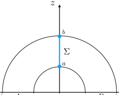
Figure 4: Entanglement wedge cross section.

In the $T\bar{T}$ deformed geometry, using the solution of the deformed geodesics (2.11), the entanglement wedge cross section becomes (see Fig. 5)

$$E_{W}^{\mu} =\frac{c}{6}\log\frac{r_{b}(\mu)}{r_{a}(\mu)}$$

$$=\frac{c}{6}\log\frac{b}{a}+\frac{c}{6}\log\left[\frac{1+z_{c}^{2}/b^{2}}{1+z_{c}^{2}/a^{2}}\right]^{1/2}.$$ (3.3)

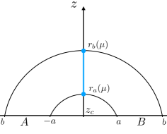
Figure 5: Deformed entanglement wedge cross section.

For $z_{c}^{2}/a^{2},\,z_{c}^{2}/b^{2}\ll 1$, it can be expanded as

$$\left(1+\frac{z_{c}^{2}}{2b^{2}}\right)\left(1-\frac{z_{c}^{2}}{2a^{2}}\right)=1-\frac{\mu c}{48\pi}\frac{b^{2}-a^{2}}{a^{2}b^{2}}+\mathcal{O}(\mu^{2}),$$ (3.4)

so for small enough deformations, the correction term of order $\mathcal{O}(\mu^{1})$ is expressed by

$$\Delta E_{W}^{\mu} \simeq\frac{c}{6}\times\left(-\frac{\mu c}{48\pi}\frac{b^{2}-a^{2}}{a^{2}b^{2}}\right)$$

$$=-\frac{\mu c^{2}}{288\pi}\frac{b^{2}-a^{2}}{a^{2}b^{2}}.$$ (3.5)

This implies that in a $T\bar{T}$ deformed CFT the corresponding EoP will decrease even for a small deformation. On the other hand, when one considers $z_{c}^{2}/a^{2},\,z_{c}^{2}/b^{2}\rightarrow\infty$,

$$E_{W}^{\mu}=\frac{c}{6}\log\left[\frac{b^{2}/z_{c}^{2}+1}{a^{2}/z_{c}^{2}+1}\right]^{1/2}\rightarrow 0,$$ (3.6)

which means the dual CFT reduces to be trivial.

3.2 Entanglement wedge cross section in BTZ blackhole

Next we also consider a finite temperature state in a holographic CFT, which corresponds to a planar BTZ black hole. The metric is given by

$$ds^{2} =\frac{1}{z^{2}}\left(-f(z)dt^{2}+\frac{dz^{2}}{f(z)}+dx^{2}\right),$$ (3.7)

$$f(z) =1-\frac{z^{2}}{z_{H}^{2}},$$ (3.8)

where the location of the blackhole horizon $z_{H}$ is related to the inverse temperature $\beta$ by $\beta=2\pi z_{H}$. This time we define a subsystem $A$ to be the interval $-l/2\leq x\leq l/2$ and $B$ to be its complement. Then, we need to consider two cases $\Sigma_{AB}^{(1)}$ and $\Sigma_{AB}^{(2)}$ described in Fig. 6. So we find that the entanglement wedge cross section will be

$$E_{W}=\frac{c}{6}\min\{2\mathcal{A}^{(1)},\,\mathcal{A}^{(2)}\},$$ (3.9)

where $\mathcal{A}^{(1)},\,\mathcal{A}^{(2)}$ are the length of $\Sigma_{AB}^{(1)}$ and $\Sigma_{AB}^{(2)}$. Similarly to the analyses in the previous section, the favored entanglement wedge cross section will be the one in which the total length of the cross section is minimal.

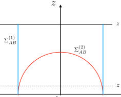
Figure 6: Entanglement wedge cross section in BTZ blackhole geometry

The length of $\Sigma_{AB}^{(1)}$ is given by

$$\mathcal{A}^{(1)} =\int_{z_{c}}^{z_{H}}\frac{1}{z\sqrt{f(z)}}dz$$

$$=\log\left(\frac{z_{H}+\sqrt{z_{H}^{2}-z_{c}^{2}}}{z_{c}}\right),$$ (3.10)

where $z_{c}=\sqrt{\mu c/24\pi}$. So we get

$$E_{W}^{(1)\,\mu}=\frac{2\mathcal{A}^{(1)}}{4G_{N}}=\frac{c}{3}\log\left(\frac{z_{H}+\sqrt{z_{H}^{2}-z_{c}^{2}}}{z_{c}}\right).$$

In this geometry, $z_{c}$ should be $0\leq z_{c}\leq z_{H}$, this means that

$$\mu c\leq\frac{6\beta^{2}}{\pi}.$$ (3.11)

This naively implies that the deformation in the thermal CFT is bounded by the temperature. Also, when $z_{c}\rightarrow z_{H}$, $\mathcal{A}^{(1)}\rightarrow 0$. If we consider $z_{c}/z_{H}\ll 1$,

$$\log\left(\frac{z_{H}+\sqrt{z_{H}^{2}-z_{c}^{2}}}{z_{c}}\right) \simeq\log\frac{2z_{H}}{z_{c}}+\log\left(1-\frac{z_{c}^{2}}{4z_{H}^{2}}\right)$$

$$=\log\left(\frac{\beta}{\pi z_{c}}\right)-\frac{\pi}{24}\frac{\mu c}{\beta^{2}}.$$ (3.12)

The first term is an ordinary contribution and $z_{c}$ here is just corresponding to a small cutoff. So, the correction term of order $\mathcal{O}(\mu^{1})$ can be written as

$$\Delta E_{W}^{(1)\,\mu}=-\frac{\pi}{72}\frac{\mu c^{2}}{\beta^{2}}.$$ (3.13)

Secondly, we consider the case of $\Sigma_{AB}^{(2)}$. For computations, let us write the BTZ black hole metric in the global coordinate:

$$ds^{2}=-\cosh^{2}\rho d\tau^{2}+d\rho^{2}+\sinh^{2}\rho d\theta^{2},$$ (3.14)

where

$$z=\frac{z_{H}}{\cosh\rho},$$ (3.15)

and so

$$\cosh\rho_{\infty}=\frac{z_{H}}{z_{c}}.$$ (3.16)

Then, the length of $\Sigma_{AB}^{(2)}$ is given by

$$\cosh\mathcal{A}^{(2)} =1+2\cosh^{2}\rho_{\infty}\sinh^{2}\frac{\pi l}{\beta}$$

$$=1+2\left(\frac{z_{H}}{z_{c}}\right)^{2}\sinh^{2}\frac{\pi l}{\beta}.$$ (3.17)

So we find that

$$\mathcal{A}^{(2)}=\log\left[1+2\left(\frac{z_{H}}{z_{c}}\right)^{2}\sinh^{2}\frac{\pi l}{\beta}\left(1+\sqrt{1+\left(\frac{z_{c}}{z_{H}}\right)^{2}\left(\sinh\frac{\pi l}{\beta}\right)^{-2}}\right)\right].$$ (3.18)

For $z_{c}/z_{H}\ll 1$, at the order of $\mathcal{O}(z_{c}/z_{H})$,

$$\mathcal{A}^{(2)} \simeq\log\left(2+4\left(\frac{z_{H}}{z_{c}}\right)^{2}\sinh^{2}\frac{\pi l}{\beta}\right)$$

$$\simeq 2\log\left(\frac{\beta}{\pi z_{c}}\sinh\frac{\pi l}{\beta}\right),$$ (3.19)

this is a well known usual result. Taking into account of the second order, we obtain

$$\mathcal{A}^{(2)}\simeq\log\left[4\left(\frac{z_{H}}{z_{c}}\right)^{2}\sinh^{2}\frac{\pi l}{\beta}+2-\frac{1}{4}\left(\frac{z_{c}}{z_{H}}\right)^{2}\left(\sinh\frac{\pi l}{\beta}\right)^{-2}\right],$$ (3.20)

where

$$\left(\frac{z_{c}}{z_{H}}\right)^{2}=\frac{\pi}{6}\frac{\mu c}{\beta^{2}}.$$ (3.21)

When $z_{c}\rightarrow z_{H}$,

$$\mathcal{A}^{(2)}=\log\left[1+2\sinh^{2}\frac{\pi l}{\beta}\left(1+\sqrt{1+\left(\sinh\frac{\pi l}{\beta}\right)^{-2}}\right)\right]\neq 0,$$ (3.22)

this means that a phase transition should occur, $\Sigma_{AB}^{(2)}\rightarrow\Sigma_{AB}^{(1)}$. The transition should occur at the point $\mathcal{A}^{(2)}=2\mathcal{A}^{(1)},$ which is

$$z_{c}^{(c)}=z_{H}\sqrt{1-\sinh^{2}\frac{\pi l}{\beta}}.$$ (3.23)

Thus, the entanglement wedge cross section is again given by

$$E_{W} =\frac{c}{6}\min\left\{2\mathcal{A}^{(1)},\;\mathcal{A}^{(2)}\right\}.$$ (3.24)

When $0\leq z_{c}\leq z_{c}^{(c)}$, $\Sigma_{AB}^{(2)}$ is realized, and when $z_{c}^{(c)}\leq z_{c}\leq z_{H}$, $\Sigma_{AB}^{(1)}$ is. One comment regarding this is that we do not change the size of the subsystem, but only the deformation parameter. This means that when we consider the $T\bar{T}$ deformation, the transition between the two entanglement wedge cross sections can occur for fixed subsystems.

Let us try to translate them into CFT language. In CFT side, the variables are interpreted through

$$z_{c}=\sqrt{\frac{\mu c}{24\pi}},~{}\beta=2\pi z_{H}.$$ (3.25)

So the transition point (3.23) is rewritten in terms of the CFT deformation parameter $\mu$ and the inverse temperature $\beta$ by

$$\mu^{(c)}c =\frac{6\beta^{2}}{\pi}\left(1-\sinh^{2}\frac{\pi l}{\beta}\right).$$ (3.26)

Recall that from $z_{c}\leq z_{H}$, the deformation parameter $\mu$ is bounded by

$$\mu c \leq\frac{6\beta^{2}}{\pi}=:\mu_{H}c.$$ (3.27)

Therefore, in CFT side we suggest that

$$0 \leq\mu c\leq\mu^{(c)}c\;\Longrightarrow\;E_{P}^{(2)\,\mu},$$ (3.28)

$$\mu^{(c)}c \leq\mu c\leq\mu_{H}c\;\Longrightarrow\;E_{P}^{(1)\,\mu}.$$ (3.29)

This implies that in thermal CFT even if one does not change the size of subsystems, the $T\bar{T}$ deformation will induce a transition of entanglement of purification. To analyze this directly from field theory side is quite tough since we do not know how to compute the entanglement of purification in general QFT. Our result provides a holographic prediction to the effect of the integrable $T\bar{T}$ deformation on the entanglement of purification in deformed CFTs.

4 Conclusion and Discussion

In this paper, we have carried out calculations of two-interval holographic entanglement entropy and holographic entanglement of purification in cutoff AdS, and also investigated the effect of the $T\bar{T}$ deformation on their phase transitions. In Sec. 2, we have studied the two-interval entanglement entropy in the cutoff AdS. Fig. 3 shows that the subsystem is getting smaller by the $T\bar{T}$ deformation. This is easy to understand in gravity side since the metric becomes small for larger $z$ and in the cutoff AdS subsystems are moving into the bulk. This is consistent with the view point of boosted CFT and its entanglement entropy [27], and it means that by the $T\bar{T}$ deformation subsystems in the field theory effectively shrink or in other words degrees of freedom in the subsystems effectively become small. A natural further study is to check the behavior of the transition in the field theory side, and evaluate how the conjecture [4] is valid and how much the Ryu-Takayanagi formula can be assumed. This should be tough since the deformed quantum field theory is no longer conformal. What we can do is full nonperturbative analysis, or perturbative expansion around the original CFT. Also, another question regarding this is a generalization to a multi-interval case. When one considers a multi-interval case, it would be interesting to study holographic mutual information and the effect of the $T\bar{T}$ deformation on monogamy relations [31].

In Sec. 3, we studied the effect of the $T\bar{T}$ deformation on the entanglement wedge cross section, which is conjectured to be dual to the entanglement of purification in the boundary field theory. Concerning this, it would be interesting to consider wormholes, or eternal black holes in the $T\bar{T}$ deformed geometry. They are originally constructed from BTZ blackhole geometry [32, 33], and have been studied by many people. The cutoff AdS, as we have seen, influences on entanglement entropy. So generically the $T\bar{T}$ deformation also affects thermo field double states, and it turns out that the $T\bar{T}$ deformation might be able to make a deformed wormhole, on whose boundary the deformed CFTs live.

We found that two-interval holographic entanglement entropy in cutoff AdS really has a correction due to the deformation, which implies that in the field theory side degrees of freedom in a subregion is decreasing by the $T\bar{T}$ deformation. Also, we investigated the entanglement wedge cross section in cutoff AdS both at zero temperature and at finite temperature. Normally, the computation of entanglement of purification in generic QFTs is a difficult problem, thus, our results provide holographic predictions. More study on holographic entanglements in this direction will play an important role in understanding of holography beyond AdS/CFT.

Acknowledgements

We would like to thank Naotaka Kubo, Kotaro Tamaoka and Koji Umemoto for valuable discussions. The author thanks the Yukawa Institute for Theoretical Physics at Kyoto University, where this work was initiated during the YITP-T-18-04 on “Strings and Fields 2018,” and also discussions during “the YITP Atoms program” were quite useful to complete this work. This work was supported by RIKEN Junior Research Associate Program.

References

- [1] J. M. Maldacena, “The Large N limit of superconformal field theories and supergravity,” Int. J. Theor. Phys. 38 (1999) 1113–1133, arXiv:hep-th/9711200 [hep-th]. [Adv. Theor. Math. Phys.2,231(1998)].
- [2] S. S. Gubser, I. R. Klebanov, and A. M. Polyakov, “Gauge theory correlators from noncritical string theory,” Phys. Lett. B428 (1998) 105–114, arXiv:hep-th/9802109 [hep-th].
- [3] E. Witten, “Anti-de Sitter space and holography,” Adv. Theor. Math. Phys. 2 (1998) 253–291, arXiv:hep-th/9802150 [hep-th].
- [4] L. McGough, M. Mezei, and H. Verlinde, “Moving the CFT into the bulk with ,” JHEP 04 (2018) 010, arXiv:1611.03470 [hep-th].
- [5] F. A. Smirnov and A. B. Zamolodchikov, “On space of integrable quantum field theories,” Nucl. Phys. B915 (2017) 363–383, arXiv:1608.05499 [hep-th].
- [6] A. Cavaglia, S. Negro, I. M. Szecsenyi, and R. Tateo, “-deformed 2D Quantum Field Theories,” JHEP 10 (2016) 112, arXiv:1608.05534 [hep-th].
- [7] A. B. Zamolodchikov, “Expectation value of composite field T anti-T in two-dimensional quantum field theory,” arXiv:hep-th/0401146 [hep-th].
- [8] I. Heemskerk and J. Polchinski, “Holographic and Wilsonian Renormalization Groups,” JHEP 06 (2011) 031, arXiv:1010.1264 [hep-th].
- [9] T. Faulkner, H. Liu, and M. Rangamani, “Integrating out geometry: Holographic Wilsonian RG and the membrane paradigm,” JHEP 08 (2011) 051, arXiv:1010.4036 [hep-th].
- [10] A. Giveon, N. Itzhaki, and D. Kutasov, “ and LST,” JHEP 07 (2017) 122, arXiv:1701.05576 [hep-th].
- [11] S. Dubovsky, V. Gorbenko, and M. Mirbabayi, “Asymptotic fragility, near AdS2 holography and ,” JHEP 09 (2017) 136, arXiv:1706.06604 [hep-th].
- [12] M. Asrat, A. Giveon, N. Itzhaki, and D. Kutasov, “Holography Beyond AdS,” Nucl. Phys. B932 (2018) 241–253, arXiv:1711.02690 [hep-th].
- [13] G. Giribet, “-deformations, AdS/CFT and correlation functions,” JHEP 02 (2018) 114, arXiv:1711.02716 [hep-th].
- [14] P. Kraus, J. Liu, and D. Marolf, “Cutoff AdS3 versus the deformation,” JHEP 07 (2018) 027, arXiv:1801.02714 [hep-th].
- [15] S. Chakraborty, A. Giveon, N. Itzhaki, and D. Kutasov, “Entanglement beyond AdS,” Nucl. Phys. B935 (2018) 290–309, arXiv:1805.06286 [hep-th].
- [16] T. Hartman, J. Kruthoff, E. Shaghoulian, and A. Tajdini, “Holography at finite cutoff with a deformation,” JHEP 03 (2019) 004, arXiv:1807.11401 [hep-th].
- [17] P. Caputa, S. Datta, and V. Shyam, “Sphere partition functions and cut-off AdS,” arXiv:1902.10893 [hep-th].
- [18] S. Ryu and T. Takayanagi, “Holographic derivation of entanglement entropy from AdS/CFT,” Phys. Rev. Lett. 96 (2006) 181602, arXiv:hep-th/0603001 [hep-th].
- [19] W. Donnelly and V. Shyam, “Entanglement entropy and deformation,” Phys. Rev. Lett. 121 no. 13, (2018) 131602, arXiv:1806.07444 [hep-th].
- [20] B. Chen, L. Chen, and P.-X. Hao, “Entanglement entropy in -deformed CFT,” Phys. Rev. D98 no. 8, (2018) 086025, arXiv:1807.08293 [hep-th].
- [21] A. Banerjee, A. Bhattacharyya, and S. Chakraborty, “Entanglement Entropy for deformed CFT in general dimensions,” arXiv:1904.00716 [hep-th].
- [22] P. Calabrese, J. Cardy, and E. Tonni, “Entanglement entropy of two disjoint intervals in conformal field theory,” J. Stat. Mech. 0911 (2009) P11001, arXiv:0905.2069 [hep-th].
- [23] P. Calabrese, J. Cardy, and E. Tonni, “Entanglement entropy of two disjoint intervals in conformal field theory II,” J. Stat. Mech. 1101 (2011) P01021, arXiv:1011.5482 [hep-th].
- [24] M. Headrick, “Entanglement Renyi entropies in holographic theories,” Phys. Rev. D82 (2010) 126010, arXiv:1006.0047 [hep-th].
- [25] T. Hartman, “Entanglement Entropy at Large Central Charge,” arXiv:1303.6955 [hep-th].
- [26] T. Takayanagi and K. Umemoto, “Entanglement of purification through holographic duality,” Nature Phys. 14 no. 6, (2018) 573–577, arXiv:1708.09393 [hep-th].
- [27] C. Park, “Holographic Entanglement Entropy in Cutoff AdS,” Int. J. Mod. Phys. A33 no. 36, (2019) 1850226, arXiv:1812.00545 [hep-th].
- [28] J. D. Brown and M. Henneaux, “Central Charges in the Canonical Realization of Asymptotic Symmetries: An Example from Three-Dimensional Gravity,” Commun. Math. Phys. 104 (1986) 207–226.
- [29] O. Aharony and T. Vaknin, “The TT* deformation at large central charge,” JHEP 05 (2018) 166, arXiv:1803.00100 [hep-th].
- [30] C. Murdia, Y. Nomura, P. Rath, and N. Salzetta, “Comments on Holographic Entanglement Entropy in TT Deformed CFTs,” arXiv:1904.04408 [hep-th].
- [31] P. Hayden, M. Headrick, and A. Maloney, “Holographic Mutual Information is Monogamous,” Phys. Rev. D87 no. 4, (2013) 046003, arXiv:1107.2940 [hep-th].
- [32] J. M. Maldacena, “Eternal black holes in anti-de Sitter,” JHEP 04 (2003) 021, arXiv:hep-th/0106112 [hep-th].
- [33] J. M. Maldacena and L. Maoz, “Wormholes in AdS,” JHEP 02 (2004) 053, arXiv:hep-th/0401024 [hep-th].