Hierarchical frequency clusters in adaptive networks of phase oscillators

Abstract

Adaptive dynamical networks appear in various real-word systems. One of the simplest phenomenological models for investigating basic properties of adaptive networks is the system of coupled phase oscillators with adaptive couplings. In this paper, we investigate the dynamics of this system. We extend recent results on the appearance of hierarchical frequency-multi-clusters by investigating the effect of the time-scale separation. We show that the slow adaptation in comparison with the fast phase dynamics is necessary for the emergence of the multi-clusters and their stability. Additionally, we study the role of double antipodal clusters, which appear to be unstable for all considered parameter values. We show that such states can be observed for a relatively long time, i.e., they are metastable. A geometrical explanation for such an effect is based on the emergence of a heteroclinic orbit.

Adaptive networks are characterized by the property that their connectivity can change in time, depending on the state of the network. A prominent example of adaptive networks are neuronal networks with plasticity, i.e., an adaptation of the synaptic coupling. Such an adaptation is believed to be related to the learning and memory mechanisms. In other real-world systems, the adaptivity plays important role as well Gross and Blasius (2008). This paper investigates a phenomenological model of adaptively coupled phase oscillators. The considered model is a natural extension of the Kuramoto system to the case with dynamical couplings. In particular, we review and provide new details on the self-organized emergence of multiple frequency-clusters.

I Introduction

One of the main motivations for studying adaptive dynamical networks comes from the field of neuroscience where the weights of the synaptic coupling can adapt depending on the activity of the neurons that are involved in the coupling Gerstner et al. (1996); Clopath et al. (2010); Gerstner et al. (2014). For instance, the coupling weights can change in response to the relative timings of neuronal spiking Markram, Lübke, and Sakmann (1997); Abbott and Nelson (2000); Caporale and Dan (2008); Lücken et al. (2016). Adaptive networks appear also in chemical Jain and Krishna (2001), biological, or social systems Gross and Blasius (2008).

This paper is devoted to a simple phenomenological model of adaptively coupled phase oscillators. The model has been extensively studied recently Kasatkin et al. (2017); Aoki and Aoyagi (2009, 2011); Kasatkin and Nekorkin (2016); Nekorkin and Kasatkin (2016); Gushchin, Mallada, and Tang (2015); Picallo and Riecke (2011); Timms and English (2014); Ren and Zhao (2007); Avalos-Gaytán et al. (2018); Berner et al. (2019a), and it exhibits diverse complex dynamical behaviour. In particular, stable multi-frequency clusters emerge in this system, when the oscillators split into groups of strongly coupled oscillators with the same average frequency. Such a phenomenon does not occur in the classical Kuramoto or Kuramoto-Sakaguchi system. The clusters are shown to possess a hierarchical structure, i.e., their sizes are significantly different Berner et al. (2019a). Such a structure leads to significantly different frequencies of the clusters and, as a result, to their uncoupling. This phenomenon is reported for an adaptive network of Morris-Lecar bursting neurons with spike-timing-dependent plasticity rule Popovych, Xenakis, and Tass (2015). In addition, the role of hierarchy and modularity in brain networks has been discussed recently Bassett et al. (2008, 2010); Lohse et al. (2014); Betzel et al. (2017); Ashourvan et al. (2019). Both features therefore seem to play a key role for real-world neural networks. Along these lines, we study a dynamical model to analyse the self-organized formation of such network structures.

In this paper, we first provide a non-technical overview of known results on multi-frequency clusters from Refs. Kasatkin et al., 2017; Berner et al., 2019a. Apart from that, we investigate the role of the time-scale separation. Particularly, we find that the slow adaptation mechanism in comparison with the fast dynamics of the oscillators is an important necessary ingredient for the emergence of stable multi-clusters. Discussing the stability, we point out that the stability analysis for the limiting case without adaptation does not provide correct stability results for arbitrarily small adaptation. In addition, the stability for one-clusters is described depending on the time-scale separation. With these results, we quantitatively relate the stability of one- with multi-frequency cluster states which goes beyond the qualitative analysis given in Ref. Berner et al., 2019a. Providing a novel result for the stability of two-clusters, the instability of evenly sized clusters is shown. Finally, we discuss the role of a special type of cluster states, called double antipodal clusters. We show that these states are unstable for all parameter values but can appear as saddles connecting synchronous and splay states in phase space. As a result, such states can be observed as a ”meta-stable” transition between the phase-synchronous and non-phase-synchronous state. Moreover, the double antipodal states are shown to play an important role for the global dynamics of the adaptive system.

The structure of the paper is as follows. Section II presents the model; Sec. III and IV provide a non-technical overview of Ref. Berner et al., 2019a on the multi-frequency cluster states and their classification. The new results are included in Sec. V-VIII. In Sec. IV we further describe one-clusters, i.e., single blocks of which the multi-clusters are composed. Section V discusses the results of Ref. Berner et al., 2019a on the stability of one- and multi-frequency clusters from a different viewpoint focusing on the influence of the time-scale separation. We provide novel rigorous results on the stability for the whole classes of antipodal, double antipodal, and $4$-phase cluster states. The stability regions for antipodal and splay-type one-clusters are explicitly described for any parameter range of the time-scale separation. In Sec. VI, the role of double antipodal states for the global dynamics of the system is discussed. The construction of multi-cluster states from one-clusters is demonstrated in Sec. VII. For the existence of multi-clusters a new upper bound for the time separation is derived. In Sec. VIII, we connect the stability properties of one- and multi-clusters. As conjectured in Ref. Berner et al., 2019a, the instability of evenly sized two-clusters of splay type are proved. For the sake of readability, the proofs for any of the statements in this section are provided in the appendix A. We end with the Conclusion.

II Model

In this article, we consider a network of $N$ adaptively coupled phase oscillators

$$\frac{d\phi_{i}}{dt} =\omega-\frac{1}{N}\sum_{j=1}^{N}\kappa_{ij}\sin(\phi_{i}-\phi_{j}+\alpha),$$ (1)

$$\frac{d\kappa_{ij}}{dt} =-\epsilon\left(\sin(\phi_{i}-\phi_{j}+\beta)+\kappa_{ij}\right),$$ (2)

where $\phi_{i}\in[0,2\pi)$ is the phase of the $i$-th oscillator ($i=1,\dots,N$) and $\omega$ the natural frequency. The oscillators interact according to the coupling structure represented by the coupling weights $\kappa_{ij}$ ($i,j=1,\dots,N$) as dynamical variables. The parameter $\alpha$ can be considered as a phase-lag of the interaction Sakaguchi and Kuramoto (1986). This paradigmatic model of an adaptive network Eqs. (1)–(2) has attracted a lot of attention recently Kasatkin et al. (2017); Aoki and Aoyagi (2009, 2011); Kasatkin and Nekorkin (2016); Nekorkin and Kasatkin (2016); Gushchin, Mallada, and Tang (2015); Picallo and Riecke (2011); Timms and English (2014); Ren and Zhao (2007); Avalos-Gaytán et al. (2018); Berner et al. (2019a). It provides a generalization of the Kuramoto-Sakaguchi model with fixed $\kappa_{ij}$ Acebrón et al. (2005); Kuramoto (1984); Omel’chenko and Wolfrum (2012); Strogatz (2000); Pikovsky and Rosenblum (2008).

The coupling topology of the network at time $t$ is characterized by the coupling weights $\kappa_{ij}(t)$. With a small parameter $0<\epsilon\ll 1$, the dynamical equation (2) describes the adaptation of the network topology depending on the dynamics of the network nodes. In the neuroscience context, such an adaptation can be also called plasticity Aoki and Aoyagi (2011). The chosen adaptation function has the form $-\sin(\phi_{i}-\phi_{j}+\beta)$ with control parameter $\beta$. With this, different plasticity rules can be modelled, see Fig. 1. For instance, for $\beta=-\pi/2$, a Hebbian-like rule is obtained where the coupling $\kappa_{ij}$ is increasing between any two phase oscillators with close phases, i.e., $\phi_{i}-\phi_{j}$ close to zero Hebb (1949); Hoppensteadt and Izhikevich (1996); Seliger, Young, and Tsimring (2002); Aoki (2015) (fire together - wire together). If $\beta=0$, the link $\kappa_{ij}$ is strengthened if the $j$-th oscillator precedes the $i$-th. Such a relationship promotes a causal structure in the oscillatory system. In neuroscience these adaptation rules are typical for spike timing- dependent plasticity Caporale and Dan (2008); Maistrenko et al. (2007); Lücken et al. (2016); Popovych, Yanchuk, and Tass (2013).

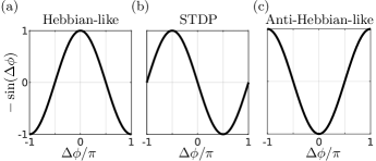
Figure 1: The plasticity function $-\sin(\Delta\phi+\beta)$ and corresponding plasticity rules are presented. (a) $\beta=-\frac{\pi}{2}$ (Hebbian), (b) $\beta=0$ (Spike timing-dependent plasticity, STDP), (c) $\beta=\frac{\pi}{2}$ (Anti-Hebbian).

Let us mention important properties of the model (1)–(2). The parameter $\epsilon\ll 1$ separates the time scales of the slowly adapting coupling weights from the fast moving phase oscillators. Further, the coupling weights are confined to the interval $-1\leq\kappa_{ij}\leq 1$ due to the fact that $d\kappa_{ij}/dt\leq 0$ for $\kappa_{ij}=1$ and $d\kappa_{ij}/dt\geq 0$ for $\kappa_{ij}=-1$, see Ref. Kasatkin et al., 2017. Due to the invariance of system (1)–(2) with respect to the shift $\phi_{i}\mapsto\phi_{i}+\psi$ for all $i=1,\dots,N$ and $\psi\in[0,2\pi)$, the frequency $\omega$ can be set to zero in the co-rotating coordinate frame $\phi\mapsto\phi+\omega t$. Finally we mention the symmetries of the system (1)–(2) with respect to the parameters $\alpha$ and $\beta$:

$$(\alpha,\beta,\phi_{i},\kappa_{ij}) \mapsto(-\alpha,\pi-\beta,-\phi_{i},\kappa_{ij}),$$

$$(\alpha,\beta,\phi_{i},\kappa_{ij}) \mapsto(\alpha+\pi,\beta+\pi,\phi_{i},-\kappa_{ij}).$$

These symmetries allow for a restriction of the analysis to the parameter region $\alpha\in[0,\pi/2)$ and $\beta\in[-\pi,\pi)$.

The Kuramoto order parameter $R_{1}$ measures the synchrony of phase oscillators $\bm{\phi}=(\phi_{1},\dots,\phi_{N})^{T}$. Correspondingly, the $l$-th moment order parameter $R_{l}$ is given by

$$R_{l}(\bm{\phi}):=\left|\frac{1}{N}\sum_{j=1}^{N}e^{\mathrm{i}l\phi_{j}}\right|$$ (3)

where $l\in\mathbb{N}$. In the following section we will use this quantity in order to characterize several dynamical states.

III Hierarchical frequency clusters

System (1)–(2) has been studied numerically in Refs. Aoki and Aoyagi, 2009, 2011; Nekorkin and Kasatkin, 2016; Kasatkin and Nekorkin, 2016; Kasatkin et al., 2017.In particular, it is shown that starting from uniformly distributed random initial condition ($\phi_{i}\in[0,2\pi)$, $\kappa_{ij}\in[-1,1]$ for all $i,j\in\left\{1,\dots,N\right\}$) the system can reach different multi-frequency cluster states with hierarchical structure. An individual cluster in the multi-cluster state consists of frequency synchronized groups of phase oscillators. In the following we discuss the structural form of these clusters. Subsequently, frequency multi-clusters states are called multi-cluster states or multi-clusters for simplicity.

Figure 2 shows a hierarchical multi-cluster state. The solution was obtained by integrating the system (1)–(2) numerically starting from uniformly distributed random initial conditions. The self-couplings $\kappa_{ii}$ are set to zero in numerical simulations, since they do not influence the relative dynamics of the system . We re-order the oscillators (after sufficiently long transient time) by first sorting the oscillators with respect to their average frequencies. After that the oscillators with the same frequency are sorted by their phases. Figure 2(a) displays the coupling matrix (right) of the multi-cluster state and a representation of the coupling structure as a network graph (left). The coupling matrix demonstrates a clear splitting into three groups. This splitting is also visible in the graph representation of the coupling network. The coupling weights between oscillators of the same group vary in a larger range than between those of different groups which are generally smaller in magnitude. The splitting into three groups is manifested in the behaviour of the phase oscillators, as well. We find that the oscillators of the same group posses the same constant frequency with possible phase lags, Fig.2(b). We call the groups of oscillators (frequency) clusters and the corresponding dynamical states multi-(frequency)cluster states.

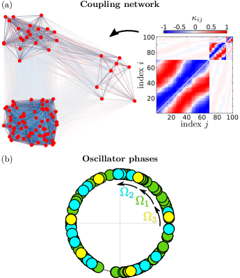
Figure 2: Three-frequency cluster of splay type at $t=10000$. (a) Coupling weights represented as a graph (left) and as a coupling matrix (right). In the graph representation, the dynamical vertices are represented by red nodes and the edges are coloured with respect to the coupling weight. Red and blue refer to positive and negative coupling weights, respectively. Light and dark colours refer to weak and strong coupling weights, respectively. (b) Distribution of the phases $\phi_{i}$ for each of the three clusters. Each node represents one oscillator and is coloured with respect to the cluster to which it belongs. Parameter values: $\epsilon=0.01$, $\alpha=0.3\pi$, $\beta=0.23\pi$, $\omega=0$, and $N=100$.

In a multi-cluster, the coupling matrix $\kappa$ can be divided into different blocks; $\kappa_{ij,\mu\nu}$ will refer to the coupling weight between the $i$-th oscillator of the $\mu$-th cluster to the $j$-th oscillator of the $\nu$-th cluster. Analogously, $\phi_{i,\mu}$ denotes the $i$-th phase oscillator in the $\mu$-th cluster. In general, the temporal behaviour for each oscillator in a $M$-cluster state takes the form

$$\phi_{i,\mu}(t)=\Omega_{\mu}t+a_{i,\mu}+s_{i,\mu}(t) \begin{split}\mu=1,\dots,M\\ i=1,\dots,N_{\mu}\end{split}$$ (4)

where $M$ is the number of clusters, $N_{\mu}$ is the number of oscillators in the $\mu$-th cluster, $a_{i,\mu}\in[0,2\pi)$ are phase lags, and $\Omega_{\mu}\in\mathbb{R}$ is the collective frequency of the oscillators in the $\mu$-th cluster. The functions $s_{i,\mu}$ are bounded.

The numerical analysis of system (1)–(2) shows the appearance of different multi-cluster states depending on particular choices of the phase lag parameters $\alpha$ and $\beta$ as well as on initial conditions. Starting from random initial conditions the system can end up in several states such as multi-clusters and chimera-like states Kasatkin et al. (2017). Figure 3 shows examples for the three types of multi-cluster states which appear dynamically in (1)–(2).

III.1 Splay type multi-clusters

The first type is called splay type multi-cluster state, see Fig. 3(a). The separation into three clusters is clearly visible in the coupling matrix, as well as a hierarchical structure in the cluster sizes. Regarding the distribution of the phases, we notice that the oscillators from each group are almost homogeneously dispersed on the circle. In fact, the phases from each cluster fulfil the condition $R_{2}(\bm{\phi}_{\mu})=0$ ($\mu=1,2,3$). Note that splay states as they are defined in several other works Nichols and Wiesenfeld (1992); Strogatz and Mirollo (1993); Choe et al. (2010) share the property $R_{1}(\bm{\phi})=0$. This property can be seen as a measure of incoherence for the oscillator phases, as well. In fact, it was shown that splay states are part of a whole family of solutions Burylko and Pikovsky (2011); Ashwin, Bick, and Burylko (2016) given by exactly $R_{1}(\bm{\phi})=0$. Further, $R_{2}(\phi)=R_{1}(2\bm{\phi})$ relates the two measures of incoherence. These facts motivate the definition of those clusters with $R_{2}(\bm{\phi})=0$ as splay-type clusters.

The temporal behaviour for all phase oscillators in the splay multi-cluster state is characterized by a constant frequency which differs for the different clusters, i.e., according to (4), $\phi_{i,\mu}(t)=\Omega_{\mu}t+a_{i,\mu}$ with $R_{2}(\bm{a}_{\mu})=0$ for all $\mu=1,2,3$ and $i=1,\dots,N_{\mu}$. In addition, the hierarchical cluster sizes are reflected in the frequencies. Oscillators of a big cluster have a higher frequency than those of smaller clusters. The coupling weights between the phase oscillators are fixed or change periodically with time depending on whether the oscillators belong to the same or different clusters, respectively. Moreover, the amplitude of coupling weights between clusters depends on the frequency difference of the corresponding clusters. The higher the frequency difference, the smaller is the amplitude. The periodic behaviour of the coupling weights between clusters is present in all types of multi-cluster states (Fig. 3(a,b,c)).

III.2 Antipodal type multi-clusters

Figure 3(b) shows another possible multi-cluster state. As in Fig. 3(a) the clusters are clearly visible and their oscillators show frequency synchronized temporal behaviour. In addition, the time series for the oscillators show periodic modulations on top of the linear growth. This additional dynamics is the same for all oscillators of the same cluster, and hence they are still temporally synchronized. We have $\phi_{i,\mu}(t)=\Omega_{\mu}t+a_{i,\mu}+s_{\mu}(t)$. In analogy to the coupling weights between the clusters, the amplitudes of the bounded function $s_{\mu}(t)$ depend on the differences of the cluster frequencies.

In contrast to the splay states, the phase distribution fulfils $R_{2}(\bm{a}_{\mu})=1$ for all $\mu=1,2,3$, see Fig 3(b), middle panel. Hence, all oscillators of a cluster have either the same phase $a_{\mu}\in[0,2\pi)$ or the antipodal phase $a_{\mu}+\pi$ such that $2a_{i,\mu}=2a_{\mu}$ modulo $2\pi$ for all $i=1,\dots,N_{\mu}$. Therefore, the clusters represented in Fig 3(b) are called antipodal type multi-cluster. Note that with this formal definition of an antipodal state, in-phase clusters belong to the class of antipodal clusters.

III.3 Mixed type multi-clusters

The third type of multi-cluster states combines the previous two types. The 2-cluster state shown in Fig. 3(c) consists of one splay cluster and one antipodal cluster. We call these states mixed type multi-cluster states. As we have seen before, the interaction of a cluster with an antipodal cluster induces a modulation $s(t)$ additional to the linear growth of the oscillator’s phase. In contrast, the interaction with a splay cluster does not introduce any modulation. Thus, the temporal dynamics of the oscillators in the antipodal cluster ($\mu=1$) have $s_{i,1}(t)\equiv 0$ while the oscillators in the splay cluster ($\mu=2$) show additional bounded modulations $s_{i,2}(t)$, see Fig. 3(c). For the oscillators of the splay cluster we plot the time series of two representatives. We notice the temporal shift in the dynamics of the two representatives of the splay cluster. The oscillators in the splay cluster are not completely temporally synchronized. More specifically we have $\phi_{i,1}(t)=\Omega_{1}t+a_{i,1}$ with $R_{2}(\bm{a}_{1})=1$ for $i=1,\dots,N_{1}$ and $\phi_{i,2}(t)=\Omega_{2}t+a_{i,2}+s_{i,2}(t)$ with $R_{2}(\bm{a}_{2})=0$ for $i=1,\dots,N_{2}$.

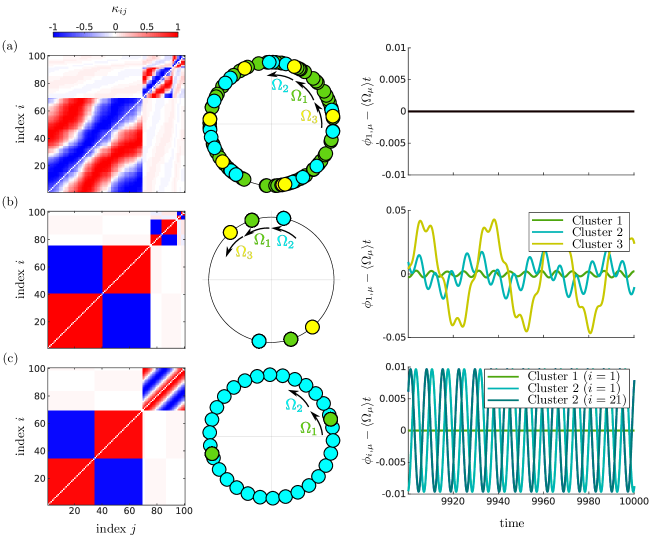
Figure 3: Three different types of multi-cluster states at $t=10000$ with $N=100$ and $\epsilon=0.01$. For all types, the coupling matrix (left), distribution of the phases (middle), and time series of representative phase oscillators from each cluster (right) are presented. In the plot of the phase distribution, each node represents one oscillator and is colored with respect to the cluster to which it belongs. The time series are shown after subtracting the average linear growth $\phi_{i,\mu}(t)-\langle\Omega_{\mu}\rangle t$. The colouring of the time series (shaded for visibility) of a representative phase oscillator from one cluster is in accordance with the pictures in the middle panel. (a) Splay type 3-cluster for $\alpha=0.3\pi$, $\beta=0.23\pi$; (b) Antipodal type 3-cluster for $\alpha=0.3\pi$, $\beta=-0.53\pi$; (c) Mixed type 2-cluster for $\alpha=0.3\pi$, $\beta=-0.4\pi$.

Despite the complexity of the three types of multi-clusters states, the structures can be broken down into simple blocks. In fact, one-cluster states of splay and antipodal type serve as building blocks in order to create more complex multi-cluster structures. In the following section we will analyse these blocks. The building of higher cluster structures will be discussed for 2-cluster states of splay type.

IV One-cluster states

As we have seen in Section III, certain one-cluster states serve as building blocks for higher multi-cluster states. In this section, we review the basic properties of one-cluster states and conclude that their shape and existence is independent of the time-separation parameter, see Ref. Berner et al., 2019a for more details.

Formally a one-cluster state is one group of frequency synchronized phase oscillators given by

$$\phi_{i}=\Omega t+a_{i}$$

with $a_{i}\in[0,2\pi)$ ($i=1,\dots,N$) and constant coupling weights

$$\kappa_{ij}=-\sin(a_{i}-a_{j}+\beta)$$ (5)

($i,j=1,\dots,N$).

Figure 4 shows three possible types of one-cluster states for the system (1)–(2). It has been shown that these are the only existing types of one-cluster states Berner et al. (2019a). The first two shown in Fig. 4(a,b) are the splay ($R_{2}(\mathbf{a})=0$) and the antipodal ($R_{2}(\mathbf{a})=1$) clusters which were already discussed in Sec. III. The third type in Fig. 4(c) consists of two groups of antipodal phase oscillators with a fixed phase lag $\psi$. We call this class of states double antipodal. As it was mentioned in Sec. III.B., the formal definition of an antipodal state includes full in-phase relation of the oscillators. Thus in extension of the typical configuration shown in Fig. 4(c), there exist double antipodal states where only three or even only two different phases are occupied. The constant $\psi$ is the unique (modulo $2\pi$) solution of the equation

$$\frac{1-q}{q}\sin(\psi-\alpha-\beta)=\sin(\psi+\alpha+\beta),$$ (6)

where $q=Q/N$ and $Q$ is the number of phase shifts $a_{i}$ such that $a_{i}\in\{0,\pi\}$. The corresponding frequencies for the three types of states are

$$\Omega=\begin{cases}\frac{1}{2}\cos(\alpha-\beta)&\mbox{if }\,R_{2}(\mathbf{a})=0,\\ \sin\alpha\sin\beta&\mbox{if }\,R_{2}(\mathbf{a})=1,\\ \frac{1}{2}\left[\cos(\alpha-\beta)-R_{2}(\mathbf{a})\cos\psi\right]&\text{if double antipodal}\end{cases}$$ (7)

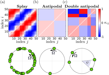
Figure 4: All possible types of one-cluster states for system Eq. (1)–(2). (a) Splay state; (b) antipodal state; (c) double antipodal state.

Note that the condition $R_{2}(\mathbf{a})=0$ gives rise to a $N-2$ dimensional family of solutions. Well-known representatives of this family are rotating-wave states which have the following form $\mathbf{a}_{k}=(0,2\pi k/N,\dots,2\pi k(N-1)/N)^{T}$ for any wave-number $k=1,\dots,N-1$. The existence as well as the explicit form for any of the three types of one-cluster states do not depend on the time separation parameter $\epsilon$. As long as $\epsilon>0$, the building blocks appear to be solutions of the system (1)–(2).

V Stability of one-cluster states

In sections III and IV a large number of co-existing multi-cluster states were discussed. As multi-clusters are constructed out of one-cluster states, studying the stability of the building blocks is of major importance. In contrast to the existence of one-cluster states, the stability of those states depend crucially on the time-separation parameter. We analyse this dependency below.

The diagram in Fig. 5 shows the regions of stability for antipodal and rotating-wave one-cluster states. The diagram is based on analytic results which has been recently found. In appendix A, we review Corollary 4.3 from Ref. Berner et al., 2019a as Proposition 1 and provide an extension to the whole class of antipodal states, see Corollary 5. Further, all other proofs are provided in the appendix A, as well.

A linear stability analysis for double antipodal states shows that they are unstable for all parameters $\alpha$ and $\beta$, see Corollary 7 in the appendix A. The role of the double antipodal clusters are discussed further in Sec. VI.

In Fig. 5 the regions of stability are presented for several values of the time separation parameter $\epsilon$. The first case in panel (a) assumes $\epsilon=0$, where the network structure is non-adaptive but fixed to the values given by the one-cluster states, i.e., $\kappa_{ij}=-\sin(a_{i}-a_{j}+\beta)$ as given in Sec. IV. The linearised system in this case is given by

$$\frac{\mathrm{d}\delta\phi_{i}}{\mathrm{d}t}=-\frac{1}{2N}\sum_{j=1}^{N}\left(\sin(\alpha-\beta)\right.\\ \left.-\sin(2(a_{i}-a_{j})+\alpha+\beta)\right)\left(\delta\phi_{i}-\delta\phi_{j}\right).$$ (8)

For the synchronized or antipodal state, the value $2a_{i}\,\text{mod }2\pi$ is the same for all $i$. Hence, the term $2(a_{i}-a_{j})$ disappears and the linearised system (8) possesses the same form as the linearised system for the synchronized state of the Kuramoto-Sakaguchi system Burylko and Pikovsky (2011) with coupling constant $\sigma(\beta)=-\sin(\beta)$. As it follows from Ref. Burylko and Pikovsky, 2011, the synchronized as well as all other antipodal states are stable for $\sigma(\beta)\cos(\alpha)>0$. The region of stability of the rotating-wave cluster has a more complex shape, see hatched area in Fig 5(a). We find large areas where both types of one-cluster states are stable simultaneously, as well as the regions where no frequency synchronized state is stable. The results shown in Fig 5(a) are in agreement with Ref. Aoki and Aoyagi, 2011, where the authors consider the case $\epsilon=0$ in order to approximate the limit case of extremely slow adaptation $\epsilon\to 0$. However, such an approach for studying the stability of clusters for small adaptation is not correct in general. As Figs. 5(b-d) show, the stability of the network with small adaptation $\epsilon>0$ is different.

The case $\epsilon=0.01$ is shown in Fig 5(b), where we observe regions for stable antipodal and rotating-wave states as well. The introduction of a small but non-vanishing adaptation changes the regions of stability significantly. The diagram in Fig 5(b) remains qualitatively the same for smaller values of $\epsilon$. This can be read of from the analytic findings presented in the Proposition 1 and Corollary 5. The changes in the stability areas are due to subtle changes in the equation which determine the eigenvalue of the corresponding linearised system. In fact, the adaptation introduces the necessary condition $\sin(\alpha+\beta)<0$ for the stability of antipodal states. Additionally, for all splay states, including rotating-wave states, the necessary condition $\sin(\alpha-\beta)+2\epsilon>0$ is introduced, see Proposition 8. This is why one can observe a non-trivial effect of adaptivity on the stability in Figs. 5. In particular, the parameter $\beta$, which determines the plasticity rule, has now a non-trivial impact on the stability of antipodal states for any $\epsilon>0$. As it can be seen in Fig. 5(b), one-cluster states of antipodal type are supported by a Hebbian-like adaption ($\beta\approx-\pi/2$) while splay states are supported by causal rules ($\beta\approx 0$). For the asynchronous region, the dynamical system (1)–(2) can exhibit very complex dynamics and show chaotic motion Kasatkin and Nekorkin (2016). This region is supported by an anti-Hebbian-like rule ($\beta\approx\pi/2$).

By increasing the parameter $\epsilon$, see Fig. 5(c,d), two observations can be made. First, the region of asynchronous dynamical behaviour is shrinking. For $\epsilon=1$, we find at least one stable one-cluster state for any choice of the phase lag parameters $\alpha$ and $\beta$. Secondly, the regions where both types of one-cluster states are stable are shrinking as well. In the limit of instant network adaptation, i.e., $\epsilon\to\infty$, the stability regions are completely separated. Both types of one-cluster states divide the whole parameter space into two areas. In this case, the boundaries are described by $\alpha+\beta=0$ and $\alpha+\beta=\pi$. This division can be seen from the analytic findings presented in Proposition 1 (Appendix A). In the case of antipodal states, the quadratic equation which determines the Lyapunov coefficients has negative roots if and only if $\epsilon+\cos(\alpha)\sin(\beta)>0$ and $\sin(\alpha+\beta)<0$. Here, even for $\epsilon>1$, the condition $\sin(\alpha+\beta)<0$ is the only remaining one. Similarly, we find $\sin(\alpha+\beta)>0$ as a condition for the stability of rotating-wave states for $\epsilon\to\infty$.

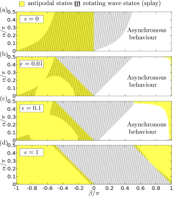
Figure 5: The regions of stability for antipodal and rotating-wave states are presented in ($\alpha,\beta$) parameter space for different values of $\epsilon$. Coloured and hatched areas refer to stable regions for these states as indicated in the legend. White areas refer to region where these one-cluster states are unstable. (a) $\epsilon=0$; (b) $\epsilon=0.01$; (c) $\epsilon=0.1$; (d) $\epsilon=1$.

VI Double antipodal states

Splay and antipodal clusters serve as building blocks for multi-cluster states. The third type, the double antipodal clusters, are not of this nature since they appear to be unstable everywhere. As unstable objects, they can still play an important role for the dynamics. Here we would like to present an example, where the double antipodal clusters become part of a simple heteroclinic network. As a result, they can be observed as metastable states in numerics.

As an example, we first analyse the system of $N=3$ adaptively coupled phase oscillators which is the smallest system with a double antipodal state. According to the definition of a double antipodal state, laid out in Sec. IV, the phases $a_{i}$ of the oscillators $\phi_{i}$ are allowed to take values from the set $\{0,\pi,\psi,\psi+\pi\}$ where $\psi$ uniquely solves Eq. (6). Further, at least one oscillator $\phi_{i}$ with $a_{i}\in\{0,\pi\}$ and one oscillator $\phi_{j}$ ($j\neq i$) with $a_{j}\in\{\psi,\psi+\pi\}$ are needed in order to represent one of the two antipodal groups. Note that for the parameters given in Fig. 6 and $N=3$, the equation (6) yields $\psi=1.602\pi$ if $a_{1},a_{2}\in\{0,\pi\}$ and $a_{3}\in\{\psi,\psi+\pi\}$.

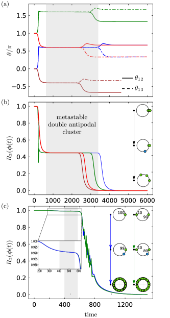
Figure 6: Heteroclinic orbits between several steady states in a system of $3$ and $100$ adaptively coupled phase oscillators. (a) The time series for the relative phases $\theta_{12}$ (solid lines) and $\theta_{13}$ (dashed lines) for $N=3$ are shown. Lines with the same colour correspond to the same trajectories. Panel (b,c) show time series for the second moment order parameter $R_{2}(\bm{\phi}(t))$ as well as a schematic illustration of the observed heteroclinic connections (right) for (b) $N=3$ and (c) $N=100$. Parameter values: $\epsilon=0.01$, $\alpha=0.4\pi$, and $\beta=-0.15\pi$.

In Fig. 6(a) we present trajectories which initially start close to antipodal clusters. The trajectories in phase space are represented by the relative coordinates $\theta_{12}=\phi_{1}-\phi_{2}$ and $\theta_{13}=\phi_{1}-\phi_{3}$. In particular, the two configurations with $(\theta_{12}=0,\theta_{13}=0)$ and $(\theta_{12}=0,\theta_{13}=\pi)$ are considered. The coupling weights are initialized according to Eq. (5). With the given parameters, the unstable manifold of the antipodal state is one-dimensional which can be determined via Proposition 1. For the numerical simulation, we perturb the antipodal state in such a way that two distinct orbits close to the unstable manifold are visible. For both configuration the two orbits are displayed in Fig. 6(a). It can be observed that after leaving the antipodal state the trajectories approach the double antipodal states before leaving it towards the direction of a splay state. With this we numerically find orbits close to ”heteroclinic”, which connect antipodal, double antipodal, and splay clusters, see schematic picture on the right in Fig. 6(b). The phase differences $\theta_{12}$ and $\theta_{13}$ at the double antipodal state agree with the solution $\psi$ of Eq. (6) or $\psi+\pi$. Figure 6(b) further justifies our statements on the heteroclinic contours. Here, we see the time series for the second moment order parameter for all trajectories in Fig. 6(b). It can be seen that in all cases we start at an antipodal cluster ($R_{2}(\bm{\phi})=1$) from which the double antipodal state ($R_{2}(\bm{\phi})\approx 0.447$, theoretical) is quickly approached. The trajectories stay close to the double antipodal cluster for approximately $2000$ time units (shaded area) before leaving the invariant set towards the splay state ($R_{2}(\bm{\phi})=0$).

As a second example we analyze a system of $N=100$ adaptively coupled phase oscillators. Here, we choose two particular antipodal states as initial condition and add a small perturbation to both. One of the states is chosen as an in-phase synchronous cluster. In both cases, the couplings weights are initialized in accordance with Eq (5). For Figure 6(c) we depict the trajectories which show a clear heteroclinic contour between antipodal, double antipodal, and splay state as in the example of three phase oscillators. We illustrate the heteroclinic connections and present $R_{2}(t)$ for the corresponding trajectories in Figure 6(c). Here, the zoomed view clearly shows that the trajectories for both initial conditions starting at an antipodal cluster ($R_{2}(\bm{\phi})=1$) again first approaches an double antipodal state ($R_{2}(\bm{\phi})\approx 0.990$, theoretical) before leaving it towards a splay state ($R_{2}(\bm{\phi})=0$). More precisely, each trajectory comes close to a particular double antipodal state for which only one oscillator has a phase in $\{\psi,\psi+\pi\}$. Remarkably, these states, also known as solitary states, have been found in a range of other systems of coupled oscillators, as well Maistrenko, Penkovsky, and Rosenblum (2014). With Proposition 4 in the Appendix, one can show that this double antipodal states have a stable manifold with co-dimension one which thus divides the phase space. Next to this fact, numerical evidence for the existence of heteroclinic connections between antipodal and double antipodal states as well as between double antipodal and the family of splay states is provided in Figure 6(c). With this, double antipodal states play an important role for the organization of the dynamics in system (1)–(2).

VII Emergence of multi-cluster states and the role of the time-separation parameter

In this section we show the importance of the time-separation parameter $\epsilon$ for the appearance of multi-cluster states. In particular, we obtain the critical value $\epsilon_{c}$ above which the multi-cluster states cease to exist. In order to shed light on the nature of multi-cluster states which are built out of one-cluster states, we review the following analytic result for two-cluster states of splay type which was explicitly derived in Ref. Berner et al., 2019a. Suppose we have two groups of splay cluster states, i.e., $R_{2}(\mathbf{a}_{\mu})=0$ for $\mu=1,2$. Then their combination leads to the following two-cluster solution of the system (1)–(2)

$$\phi_{i,1}(t) =\Omega_{1}t+a_{i,1},\quad i=1,\dots,N_{1}$$

$$\phi_{i,2}(t) =\Omega_{2}t+a_{i,2},\quad i=1,\dots,N_{2}$$

$$\kappa_{ij,\mu\mu}(t) =-\sin(a_{i,\mu}-a_{j,\mu}+\beta),\quad\mu=1,2$$

$$\kappa_{ij,\mu\nu}(t) =-\rho_{\mu\nu}\sin(\Delta\Omega_{\mu\nu}t+a_{i,\mu}-a_{j,\nu}+\beta-\psi_{\mu\nu}),$$

where $\mu\neq\nu$, $\Delta\Omega_{\mu\nu}:=\Omega_{\mu}-\Omega_{\nu}$, $\psi_{\mu\nu}:=\arctan(\Delta\Omega_{\mu\nu}/\epsilon),$

$$\rho_{\mu\nu}:=\left(1+\left(\Delta\Omega_{\mu\nu}/\epsilon\right)^{2}\right)^{-\frac{1}{2}},$$

$$\Omega_{\mu}=\frac{1}{2}\left(n_{\mu}\cos(\alpha-\beta)+\rho_{\mu\nu}(1-n_{\mu})\cos(\alpha-\beta+\psi_{\mu\nu})\right),$$

$$\left(\Delta\Omega_{12}\right)_{1,2}=\frac{1}{2}\left(n_{1}-\frac{1}{2}\right)\cos(\alpha-\beta)\\ \pm\frac{1}{2}\sqrt{\left(n_{1}-\frac{1}{2}\right)^{2}\cos^{2}(\alpha-\beta)-2\epsilon(2\epsilon+\sin(\alpha-\beta))},$$ (9)

and $n_{1}:=N_{1}/N$.

It is quite remarkable that in case of splay-type clusters the multi-cluster solution can be explicitly given. For a proof we refer the reader to Ref. Berner et al., 2019a.

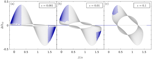
Figure 7: All possible one- and two-cluster solutions of splay type of system (1)–(2). For fixed relative size of the first cluster $n_{1}$, the frequency differences $\Delta\Omega_{12}(\beta)$ are displayed as a function of the system parameter $\beta$ corresponding to Eq. (9). The dashed lines (gray) indicate unstable solutions while the solid lines (blue) indicate stable solutions. Parameter values $N=50$ and $\alpha=0.3\pi$ are fixed for all panels.

With this, we can study directly the role of several parameters for the existence of multi-cluster states. In Figure 7, solutions for Eq. (9) are presented depending on the parameter $\beta$. The number of oscillators in the system is chosen as $N=50$. Each line $\Delta\Omega_{12}(\beta)$ in Fig. 7 represents a frequency difference of two clusters for which the two-cluster state of splay type exists with fixed relative number $n_{1}$ of oscillators in the first cluster. Note that the number of possible two-cluster states increases proportionally to the total number of oscillators $N$. Different panels show solutions for different values of $\epsilon$. We note that the existence of those two-cluster states depends only on the difference of $\gamma:=\alpha-\beta$, see Eq. (9). The necessary condition for the existence of a two-cluster state reads

$$\left(n_{1}-\frac{1}{2}\right)^{2}\cos^{2}\gamma>2\epsilon(2\epsilon+\sin\gamma).$$ (10)

From Eq. (10) we immediately see that the value of the time separation parameter $\varepsilon$ in system (1)–(2) is important for the existence of the multi-cluster states. This dependence is in contrast to the findings for one-cluster states. First of all, note that the left hand side of condition (10) is positive for $\gamma\neq\pm\pi/2$. Hence, for all parameters, there is a critical value $\epsilon_{c}$ such that there exists no two-cluster state for $\epsilon>\epsilon_{c}$. Explicitly, we have

$$\epsilon_{c}=-\frac{1}{4}\sin\gamma+\frac{1}{2}\sqrt{\frac{1}{4}\sin^{2}\gamma+\left(n_{1}-\frac{1}{2}\right)^{2}\cos^{2}\gamma},$$ (11)

which is illustrated in Fig. 8. The figure shows the critical value $\epsilon_{c}$ depending on the parameter $\gamma$ for different values of $n_{1}$. The function possesses a global maximum with $\epsilon_{c}=0.5$. This means that there is a particular requirement on the time separation in order to have two-cluster states of splay type. Indeed, the adaptation of the network has to be at most half as fast as the dynamics of the oscillatory system.

Further let us remark that the two-cluster state with equally sized clusters $n_{1}=0.5$ exists only for $\alpha-\beta\in(\pi,2\pi)$, i.e., $\epsilon_{c}=0$ for all $\alpha-\beta\in[0,\pi]$.

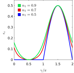
Figure 8: For the case of two-cluster states of splay type, the critical value $\epsilon_{c}$ of time-separation parameter $\epsilon$ is plotted as a function of $\gamma=\alpha-\beta$ for different cluster sizes $n_{1}=N_{1}/N$. The function is given explicitly by Eq. (11).

In Sec. III we discussed that the combination of one-cluster states to a multi-cluster state can result in modulated dynamics of the oscillators additional to the linear growth. In fact, this additional temporal behavior is due to the interaction of the clusters. As we see in Fig. 3(a), oscillators interacting with a splay-type cluster will not be forced to perform additional dynamics. This is the reason why we are able to derive a closed analytic expression for multi-cluster states of splay type. It is possible to determine the frequencies explicitly as in Eq. (9). Therefore, here the interaction between cluster causes only changes in the collective frequencies which are small whenever $\epsilon$ is small.

In contrast to splay clusters, the interaction with antipodal cluster leads to bounded modulation of the oscillator dynamics besides the constant-frequency motion. The modulations scale with $\epsilon$ and hence depend on the time-separation parameter. More rigorous results can be found in Ref. Berner et al., 2019a. In case of a mixed type two-cluster state, both interaction phenomena are present. The oscillators in the antipodal cluster interact with the splay cluster leading to no additional modulation. On the contrary, the phase oscillators of the splay cluster get additional modulation via the interaction with the antipodal cluster.

The one-cluster states of any size apparently serve as building blocks for multi-cluster states. However, not all possible multi-cluster states are stable even though the building blocks are. The next section is devoted to this question of stability.

VIII Stability of multi-cluster states

As mentioned above, the stability of one-cluster states is important for the stability of multi-cluster states. For two weakly coupled clusters, the stability of one-clusters serves as a necessary condition for the stability of the two-cluster state. In figure 7 the possible two-clusters of splay type are plotted. In addition, for each of these solutions the stability is analysed numerically. For this, we initialize the system (1)–(2) on the corresponding two-cluster state and run the simulation for $t=10000$ time units. After the simulation, we compare the initial condition with the final state in order to determine the stability. For each parameter value $\beta$ we colour the line blue (solid line) whenever the two-cluster state is stable. Otherwise, the line is gray (dashed line). An additional line at $\Delta\Omega_{12}=0$ is plotted corresponding to the one-cluster solution. The stability of the one-cluster solution is determined analytically as in Fig. 5. We notice that for $\epsilon=0.001$ a stable two-cluster state exists for almost every relative cluster size $n_{1}$, while this is not true for $\epsilon=0.01$ and even more so for $\epsilon=0.1$.

Another observation from Figs. 7(a),(b) is that the possible $\beta$-values where the two-cluster states can be stable mainly correspond to the $\beta$ values where the one-cluster state is stable. This is true for small values of $\epsilon$, however, a careful inspection of Fig. 7(c) for the case of larger $\epsilon$, here $\epsilon=0.1$, shows that some two-cluster states appear to be stable for a parameter region where the corresponding one-cluster state is unstable. This can be explained as follows. According to $\eqref{eq:PhiDGL_general}$, in the case of one-cluster states, the inter-cluster interactions are summed over all $N$ oscillators of the whole system. Additionally, the interactions are scaled with the factor $1/N$. Therefore, the total interaction scales with $1$. For two-cluster states, the inter-cluster interactions for each individual cluster are only a sum over the $N_{\mu}$ ($\mu=1,2$) oscillators whereas the scaling remains $1/N$. Hence, the total inter-cluster interaction scales with $n_{\mu}=N_{\mu}/N$, the relative size of the cluster. Therefore, the effective oscillatory system, when neglecting the interaction to the other cluster, reads

$$\frac{\mathrm{d}\phi_{i,\mu}}{\mathrm{d}t} =-\frac{n_{\mu}}{N_{\mu}}\sum_{j=1}^{N_{\mu}}\kappa_{ij,\mu\mu}\sin(\phi_{i,\mu}-\phi_{j,\mu}+\alpha),$$

$$\frac{\mathrm{d}\kappa_{ij,\mu\mu}}{\mathrm{d}t} =-\epsilon\left(\kappa_{ij,\mu\mu}+\sin(\phi_{i,\mu}-\phi_{j,\mu}+\beta)\right).$$

This system is equivalent to  (1)–(2) with $N_{\mu}$ oscillators by rescaling $\epsilon\mapsto\epsilon/n_{\mu}$. Thus, the stability of the inter-cluster system has to be evaluated with respect to the rescaled effective parameter $\epsilon_{\text{eff}}:=\epsilon/n_{\mu}$. Since $n_{\mu}<1$ for $\mu=1,2$, we have $\epsilon_{\text{eff}}>\epsilon$. As we have discussed, the stability for the one-cluster changes with increasing $\epsilon$. With this, the influence of the cluster size as well as the slight boundary shift in the regions of stability, see Fig. 7, can be explained.

Finally, we note why the equally-sized splay-clusters are not found to be stable. Indeed, from Eq. (9) we know that $2\epsilon+\sin(\alpha-\beta)<0$ is a necessary condition to have such equally-sized ($n_{1}=1/2$) clusters. However, any one-cluster splay state is unstable for $2\epsilon+\sin(\alpha-\beta)<0$ by Proposition 8 in Appendix A.

IX Conclusion

In summary, we have studied a paradigmatic model of adaptively coupled phase oscillators. It is well known that various models of weakly coupled oscillatory systems can be reduced to coupled phase oscillators. Our study has revealed the impact of synaptic plasticity upon the collective dynamics of oscillatory systems. For this, we have implemented a simplified model which is able to describe the slow adaptive change of the network depending on the oscillatory states. The slow adaptation is controlled by a time-scale separation parameter.

We have described the appearance of several different frequency cluster states. Starting from random initial conditions, our numerical simulations show two different types of states. These are the splay and the antipodal type multi-cluster states. A third mixed type multi-cluster state is found by using mathematical methods described in detail in Berner et al. (2019a). For all these states the collective motion of oscillators, the shape of the network, and the interaction between the frequency clusters is presented in detail. It turns out that the oscillators are able to form groups of strongly connected units. The interaction between the groups is weak compared to the interaction within the groups. The analysis of multi-cluster states reveals the building blocks for these states.

In particular, the following three types of relative equilibria form building blocks for multi-cluster states: splay, antipodal, and double antipodal. In order to understand the stability of the frequency cluster states, we perform a linear stability analysis for the relative equilibria. The stability of these states is rigorously described, and the impact of all parameters is shown. We prove that the double antipodal states are unstable in the whole parameter range. They appear to be saddle-points in the phase space which therefore cannot be building blocks for higher multi-cluster states. While the time-scale separation has no influence upon their existence, it plays an important role for the stability the relative equilibria. The regions of stability in parameter space are presented for different choices of the time-scale separation parameter. The singular limit ($\epsilon\to 0$) and the limit of instantaneous adaptation are analyzed. The latter shows that the stability region of the splay and the antipodal states divide the whole space into two equally sized regions without intersection. Instantaneous adaption cancels multistability of these states. The consideration of the singular limit shows that it differs from the case of no adaptation. Therefore, even for very slow adaptation, the oscillatory dynamics alone is not sufficient to describe the stability of the system.

Subsequently, the role of double antipodal states is discussed. We find that in a system of $3$ oscillators these states are transient states in a small heteroclinic network between antipodal and splay states. They appear to be metastable, i.e. observable for a relative long time and therefore are physically important transient states. Moreover an additional analysis for an ensemble of $100$ phase oscillators has revealed the importance of the double antipodal states for the global dynamics of the whole system.

For the splay clusters we analytically show the existence of two-cluster states. Remarkably, while the existence of the one-cluster states does not depend on the time-scale separation parameter, the multi-cluster states crucially depend on the time-scale separation. In fact, we provide an analysis showing that there exists a critical value for the time-scale separation. Moreover, we show that in the case of two-cluster states of splay type the adaption of the coupling weights must be at most half as fast as the dynamics of the oscillators. This fact is of crucial importance for comparing dynamical scenarios induced by short-term or long-term plasticity Fröhlich (2016).

The stability of two-cluster states is analyzed numerically and presented for different values of the time-scale separation parameter. By assuming weakly interacting clusters, we describe the stability of the two-cluster with the help of the analysis of one-cluster states. The simulations show that there are no stable two-cluster states with clusters of the same size. We provide an argument to understand this property of the system.

Appendix A Stability of one-cluster states

In order to study the local stability of one-cluster solutions described in Sec. IV, we linearise the system of differential equations (1)–(2) around the phase locked states described by $\phi_{i}=\Omega t+a_{i}$ and $\kappa_{ij}=-\sin(a_{i}-a_{j}+\beta)$. We obtain the following linearised system

$$\frac{d}{dt}\delta\phi_{i}=\frac{1}{2N}\sum_{j=1}^{N}\sin(\beta-\alpha)\left(\delta\phi_{i}-\delta\phi_{j}\right)\\ +\frac{1}{2N}\sum_{j=1}^{N}\cos(2(a_{i}-a_{j})+\alpha+\beta)\left(\delta\phi_{i}-\delta\phi_{j}\right)\\ -\frac{1}{N}\sum_{j=1}^{N}\sin(a_{i}-a_{j}+\alpha)\delta\kappa_{ij},$$ (12)

and

$$\frac{d}{dt}\delta\kappa_{ij}=-\epsilon\left(\delta\kappa_{ij}+\cos(a_{i}-a_{j}+\beta)\left(\delta\phi_{i}-\delta\phi_{j}\right)\right),$$ (13)

Note that this set of equations can be brought into the following block form

$$\frac{\mathrm{d}}{\mathrm{d}t}\begin{pmatrix}\delta\bm{\phi}\\ \delta\kappa\end{pmatrix}=\begin{pmatrix}A&B\\ C&-\epsilon\mathbb{I}_{N^{2}}\end{pmatrix}\begin{pmatrix}\delta\bm{\phi}\\ \delta\kappa\end{pmatrix}$$ (14)

where $\left(\delta\bm{\phi}\right)^{T}=\left(\delta\phi_{1},\dots,\delta\phi_{N}\right)$, $\left(\delta\kappa\right)^{T}=\left(\delta\kappa_{11},\dots,\delta\kappa_{1N},\delta\kappa_{21},\dots,\delta\kappa_{NN}\right)$, $B=\begin{pmatrix}B_{1}&\cdots&B_{N}\end{pmatrix}$, $C=\begin{pmatrix}C_{1}\\ \vdots\\ C_{N}&\\ \end{pmatrix}$, and $A$, $B_{n}$, $C_{n}$ are $N\times N$ matrices with $n=1,\dots,N$. The elements of the block matrices read

$$a_{ij} =\begin{cases}\!\begin{aligned} -\frac{1}{2}\sin(\alpha-\beta)-\frac{1}{N}\sin(\beta)\cos(\alpha)\\ +\frac{1}{2N}\sum_{k=1}^{N}\sin(2(a_{i}-a_{k})+\alpha+\beta),\end{aligned}&i=j\\ \frac{1}{2N}\left(\sin(\alpha-\beta)-\sin(2(a_{i}-a_{j})+\alpha+\beta)\right),&i\neq j\end{cases}$$

$$b_{ij;n} =\begin{cases}-\frac{1}{N}\sin(a_{n}-a_{j}+\alpha),&i=n\\ 0,&\text{otherwise}\end{cases}$$

$$c_{ij;n} =\begin{cases}0,&j=n,i=j\\ -\epsilon\cos(a_{n}-a_{i}+\beta),&j=n,i\neq j\\ \epsilon\cos(a_{n}-a_{i}+\beta),&j\neq n,i=j\\ 0,&\text{otherwise}\end{cases}.$$

Throughout this appendix we will make use of Schur’s complement Boyd and Vandenberghe (2004) in order to simplify characteristic equations. In particular, any $m\times m$ matrix $M$ in the $2\times 2$ block form can be written as

$$M=\begin{pmatrix}A&B\\ C&D\end{pmatrix}\\ =\begin{pmatrix}\mathbb{I}_{p}&BD\\ 0&\mathbb{I}_{q}\end{pmatrix}\begin{pmatrix}A-BD^{-1}C&0\\ 0&D\end{pmatrix}\begin{pmatrix}\mathbb{I}_{p}&0\\ D^{-1}C&\mathbb{I}_{q}\end{pmatrix}$$ (15)

where $A$ is a $p\times p$ matrix and $D$ is an invertible $q\times q$ matrix. The matrix $A-BD^{-1}C$ is called Schur’s complement. A simple formula for the determinant of $M$ can be derived with this decomposition in (15)

$$\det(M) =\det(A-BD^{-1}C)\cdot\det(D).$$

This result is important for the subsequent stability analysis. Note that in the following an asterisk indicates the complex conjugate.

Proposition 1.

Suppose we have $\mathbf{a}_{k}=(0,\frac{2\pi}{N}k,\dots,(N-1)\frac{2\pi}{N}k)^{T}$ and the characteristic equation of the linear system (12)–(13) then the set of eigenvalues $L$ are as follows.

1. (in-phase and anti-phase synchrony) If $k=0$ or $k=N/2$,

   $$L=\left\{\left(0\right)_{\text{1}},\left(-\epsilon\right)_{(N-1)N+1},\left(\lambda_{1}\right)_{N-1},\left(\lambda_{2}\right)_{N-1}\right\}$$

   where $\lambda_{1}$ and $\lambda_{2}$ solve $\lambda^{2}+\left(\epsilon-\cos(\alpha)\sin(\beta)\right)\lambda-\epsilon\sin(\alpha+\beta)=0$.

2. (incoherent rotating-wave) If $k\neq 0,N/2,N/4,3N/4,$ the spectrum is

   $$L=\left\{\left(0\right)_{N-2},\left(-\epsilon\right)_{(N-1)N+1},\left(-\frac{\sin(\alpha-\beta)}{2}-\epsilon\right)_{N-3},\right.\\ \left.\left(\vartheta_{1}\right)_{1},\left(\vartheta_{2}\right)_{1},\left(\vartheta_{1}^{*}\right)_{1},\left(\vartheta_{2}^{*}\right)_{1}\right\}$$

   where $\vartheta_{1}$ and $\vartheta_{2}$ solve $\vartheta^{2}+\left(\epsilon+\frac{1}{2}\sin(\alpha-\beta)-\frac{1}{4}\mathrm{i}e^{\mathrm{i}(\alpha+\beta)}\right)\vartheta-\frac{\epsilon}{2}\mathrm{i}e^{\mathrm{i}(\alpha+\beta)}=0$.

3. (4-rotating-wave state) If $k=N/4,3N/4$, the spectrum is

   $$L=\left\{\left(0\right)_{N-1},\left(-\epsilon\right)_{(N-1)N+1},\right.\\ \left.\left(-\frac{\sin(\alpha-\beta)}{2}-\epsilon\right)_{N-2},\left(\lambda_{1}\right)_{1},\left(\lambda_{2}\right)_{1}\right\}$$

   where $\lambda_{1}$ and $\lambda_{2}$ solve $\lambda^{2}+\left(\epsilon+\sin(\alpha)\cos(\beta)\right)\lambda+\epsilon\sin(\alpha+\beta)=0.$

Here, the multiplicities for each eigenvalue are given as subscripts.

Proof.

The proof can be found in Ref Berner et al., 2019a. ∎

So far, we have found the Lyapunov coefficients for the rotating-wave states. The following two Lemmata are needed to describe the stability of antipodal, $4$-phase-cluster, and double antipodal states as well.

Lemma 2.

Suppose $M$ is a block square matrix of the form

$$M =\left(\begin{array}[]{cc}A&m_{1}\hat{1}_{p,q}\\ m_{2}\hat{1}_{q,p}&B\end{array}\right)$$

where $A$ is a circulant $p\times p$ matrix, $B$ is a circulant $q\times q$ matrix, $\hat{1}_{p,q}$ is $p\times q$ where all entries are $1$ and $m_{1},m_{2}\in\mathbb{R}$. Then the eigenvector-eigenvalue pairs are given by

$$\left(\lambda_{k}^{0},\dots,\lambda_{k}^{p-1},0,\dots,0\right)^{T},\,\mu_{k}=\sum_{l=0}^{p-1}a_{1\left(1+l\right)}\lambda_{k}^{l}$$ (16)

$$\left(0,\dots,0,\rho_{l}^{0},\dots,\rho_{l}^{q-1}\right)^{T},\,\nu_{l}=\sum_{l=0}^{q-1}b_{1\left(1+l\right)}\rho_{l}^{l}$$ (17)

$$\left(1,\dots,1,a_{1},\dots a_{1}\right)^{T},\,\bar{\mu}=\mu_{0}+m_{1}qa_{1}$$ (18)

$$\left(1,\dots,1,a_{2},\dots,a_{2}\right)^{T},\,\bar{\nu}=\mu_{0}+m_{1}qa_{2}$$ (19)

with $\lambda_{k}=e^{\mathrm{i}\frac{2\pi}{p}k}$ and $\rho_{l}=e^{\mathrm{i}\frac{2\pi}{q}l}$ for $k=1,\dots,p-1$ and $l=1,\dots,q-1$, respectively, and $a_{1}$ and $a_{2}$ solve the equation

$$a^{2}+\frac{\mu_{0}-\nu_{0}}{m_{1}q}a-\frac{m_{2}p}{m_{1}q} =0$$

with $\mu_{0}=\sum_{j=1}^{p}a_{1j}$ and $\nu_{0}=\sum_{j=1}^{q}b_{1j}$.

Proof.

We can prove the Lemma by direct calculation and find

$$M\left(\lambda_{k}^{0},\dots,\lambda_{k}^{p-1},0,\dots,0\right)^{T}\\ =\left(\begin{array}[]{c}A\left(\lambda_{k}^{0},\dots,\lambda_{k}^{p-1}\right)^{T}m_{2}\sum_{l=0}^{p-1}\lambda_{k}^{l}\end{array}\right)\\ =\mu_{k}\left(\lambda_{k}^{0},\dots,\lambda_{k}^{p-1},0,\dots,0\right)^{T}.$$

Here, we use that $A$ is a circulant matrix and that $\sum_{l=0}^{p-1}\lambda_{k}^{l}=0$ for all $k=1,\dots,p-1$. Analogous arguments hold for (17). The last two eigenvector-eigenvalue pairs (18)–(19) can be obtained by

$$M\left(1,\dots,1,a,\dots,a\right)^{T}\\ =\left(\begin{array}[]{c}A\left(1,\dots,1\right)^{T}+m_{1}qa\left(1,\dots,1\right)^{T}\\ \frac{m_{2}p}{a}\left(1,\dots,1\right)^{T}+aB\left(1,\dots,1\right)^{T}\end{array}\right)\\ =\left(\begin{array}[]{c}\mu_{0}+m_{1}qa\\ \frac{m_{2}p}{a}+\nu_{0}\end{array}\right)\left(1,\dots,1,a,\dots,a\right)^{T}$$

which solves the eigenvalue problem if $a$ is chosen to be either $a_{1}$ or $a_{2}$. ∎

Lemma 3.

Suppose we have a phase locked state with phases $a_{i}\in[0,2\pi)$. Then, the solution for the characteristic equations corresponding to the linearised system (12)–(13) are given by $\lambda=-\epsilon$ with multiplicity $N^{2}-N$ and by the solution of the following set of equations

$$\det\left(\left(A-\lambda\mathbb{I}_{N}\right)\left(\epsilon+\lambda\right)+BC\right)=0.$$

Proof.

Applying Schur’s decomposition (15) to the linearised system in the block form (14) yields the result. ∎

Proposition 4.

Suppose we have a state with phases $a_{i}\in\{0,\pi,\psi,\psi+\pi\}$ where $i=1,\dots,N$. Further set $q_{1}=Q_{1}/N$ and $q_{2}=Q_{2}/N$, where $Q_{1}$ and $Q_{2}$ denote the numbers of phases which are either $0$ or $\pi$ and $\psi$ or $\psi+\pi$, respectively. Then, the linear system (12)–(13) possesses the following set $L$ of eigenvalues

$$L=\left\{\left(0\right)_{\text{1}},\left(-\epsilon\right)_{(N-1)N+1},\left(\lambda_{1}\right)_{N_{1}-1},\left(\lambda_{2}\right)_{N_{1}-1},\right.\\ \left.\left(\vartheta_{1}\right)_{N_{2}-1},\left(\vartheta_{2}\right)_{N_{2}-1},\left(\rho_{1}\right)_{1},\left(\rho_{2}\right)_{1}\right\}$$

where $\lambda_{1}$ and $\lambda_{2}$ solve

$$\lambda^{2}+\frac{1}{2}\left(\sin(\alpha-\beta)-q_{1}\sin(\alpha+\beta)\right.\\ \left.-q_{2}\sin(-2\psi+\alpha+\beta)+2\epsilon\right)\lambda\\ -\epsilon q_{1}\sin(\alpha+\beta)-\epsilon q_{2}\sin(-2\psi+\alpha+\beta)=0,$$

$\vartheta_{1}$ and $\vartheta_{2}$ solve

$$\vartheta^{2}+\frac{1}{2}\left(\sin(\alpha-\beta)-q_{1}\sin(2\psi+\alpha+\beta)\right.\\ \left.-q_{2}\sin(\alpha+\beta)+2\epsilon\right)\vartheta\\ -\epsilon q_{1}\sin(2\psi+\alpha+\beta)-\epsilon q_{2}\sin(\alpha+\beta)=0,$$

as well as $\rho_{1}$ and $\rho_{2}$ solve

$$\rho^{2}+\frac{1}{2}\left(\sin(\alpha-\beta)-q_{1}\sin(2\psi+\alpha+\beta)\right.\\ \left.-q_{2}\sin(-2\psi+\alpha+\beta)+2\epsilon\right)\rho\\ -\epsilon q_{1}\sin(2\psi+\alpha+\beta)-\epsilon q_{2}\sin(-2\psi+\alpha+\beta)=0.$$

The multiplicities for each eigenvalue are given as subscripts.

Proof.

For an arbitrary solution of the form $\phi_{i}=\Omega t+a_{i}$ we consider the linearised system (12)–(13) in the block form (14) and apply Lemma 3. The elements of the second term $D:=BC$ of Schur’s complement are then

$$d_{ij} =-\frac{\epsilon}{2N}\left(\sin(\alpha-\beta)+\sin(2(a_{i}-a_{j})+\alpha+\beta)\right)$$

if $i\neq j$ and

$$d_{ii}=\epsilon\left(\frac{1}{2}\sin(\alpha-\beta)-\frac{1}{N}\sin(\alpha)\cos(\beta)\right.\\ \left.+\frac{1}{2N}\sum_{j=1}^{N}\sin(2(a_{i}-a_{j})+\alpha+\beta)\right).$$

Defining the matrix $M:=\left(A-\lambda\mathbb{I}_{N}\right)\left(\epsilon+\lambda\right)+D$ we get

$$m_{ij} =\begin{cases}-\lambda^{2}+(a_{ii}-\epsilon)\lambda+\epsilon a_{ii}+d_{ii}&i=j\\ \lambda a_{ij}+\epsilon a_{ij}+d_{ij}.&i\neq j\end{cases}$$

Using the assumption for the phases $a_{i}$, then one group of oscillators (group $I$) have $a_{i}\in\{0,\pi\}$ and the remaining $Q_{2}$ oscillators (group $II$) have $a_{i}=\{\psi,\psi+\pi\}$. Putting this into the definition of $m_{ij}$, we find that the whole square matrix $M$ can be written as

$$M =\left(\begin{array}[]{cc}\overbrace{\begin{array}[]{cccc}m_{I}&\bar{m}&\cdots&\bar{m}\\ \bar{m}&\ddots&\ddots&\vdots\\ \vdots&\ddots&\ddots&\bar{m}\\ \bar{m}&\cdots&\bar{m}&m_{I}\end{array}}^{Q_{1}\times Q_{1}}&\begin{array}[]{c}m_{1}\hat{1}_{Q_{1},Q_{2}}\end{array}\\ \begin{array}[]{c}m_{2}\hat{1}_{Q_{2},Q_{1}}\end{array}&\underbrace{\begin{array}[]{cccc}m_{II}&\bar{m}&\cdots&\bar{m}\\ \bar{m}&\ddots&\ddots&\vdots\\ \vdots&\ddots&\ddots&\bar{m}\\ \bar{m}&\cdots&\bar{m}&m_{II}\end{array}}_{Q_{2}\times Q_{2}}\end{array}\right)$$

where $m_{1}$, $\bar{m}$, $m_{I}$, and $m_{II}$ are real values which depend on all the system parameters $\alpha$, $\beta$, $\epsilon$ and additionally on $\psi$ and $\lambda$. Note that all diagonal blocks are circulant matrices. The determinant is invariant under basis transformations which is why we diagonalize the matrix $M$ and therewith derive equations for the values $\lambda$. In order to do so, we look for the eigenvalues of $M$ determined by the characteristic equation

$$\det\left(M-\mu\mathbb{I}_{N}\right) =0.$$

Due to the structure of $M$ we can apply Lemma 2 and find the following set of eigenvalues

$$\mu_{k} =-\lambda^{2}-\frac{1}{2}(\sin(\alpha-\beta)-q_{1}\sin(\alpha+\beta)-q_{2}\sin(-2\psi+\alpha+\beta)+2\epsilon)\lambda+\epsilon q_{1}\sin(\alpha+\beta)+\epsilon q_{2}\sin(-2\psi+\alpha+\beta)$$

for $k=1,\dots,Q_{1}-1.$ Analogously, we obtain the equations for $\nu_{k}$ ($k=1,\dots,Q_{2}-1$) where $m_{I}$ is substituted with $m_{II}$. The two other eigenvalue are given by $\bar{\mu}=\mu_{0}+m_{1}Q_{2}a_{1}$ and $\bar{\nu}=\mu_{0}+m_{1}Q_{2}a_{2}$, respectively, where

$$\mu_{0} =m_{I}+(Q_{1}-1)\bar{m}$$

and $a_{1,2}$ are given by

$$a^{2}+\frac{\left(m_{I}-m_{II}\right)+\left(Q_{1}-Q_{2}\right)\bar{m}}{m_{1}Q_{2}}a-\frac{m_{2}Q_{1}}{m_{1}Q_{2}} =0.$$

Considering the row sums of $M$ we find that all agree with $-\lambda^{2}-\epsilon\lambda$ and therefore $\bar{\mu}=-\lambda^{2}-\epsilon\lambda$. Resulting from this $a_{1}=-\left(\lambda^{2}+\epsilon\lambda+\mu_{0}\right)/m_{1}Q_{2}=1$. Hence,

$$a_{2} =\frac{\left(m_{II}-m_{I}\right)+\left(Q_{2}-Q_{1}\right)\bar{m}}{m_{1}Q_{2}}-1$$

and we find

$$\bar{\nu} =m_{II}+\left(Q_{2}-1\right)\bar{m}-m_{1}Q_{2}$$

$$=-\lambda^{2}-\frac{1}{2}(\sin(\alpha-\beta)-q_{1}\sin(2\psi+\alpha+\beta)$$

$$-q_{2}\sin(-2\psi+\alpha+\beta)+2\epsilon)\lambda$$

$$+\epsilon q_{1}\sin(2\psi+\alpha+\beta)+\epsilon q_{2}\sin(-2\psi+\alpha+\beta)$$

After diagonalizing the matrix $M$ the determinant can be easily written as

$$\det(M) =\bar{\mu}\cdot\mu_{1}\cdot\dots\cdot\mu_{N_{1}-1}\cdot\bar{\nu}\cdot\nu_{1}\cdot\dots\cdot\nu_{N_{2}-1}.$$

Therewith, finding $\lambda^{\prime}s$ such that at least one of the eigenvalues of $M$ vanishes solves the initial eigenvalue problem. ∎

We will now sum up the results with the following corollaries

Corrolary 5.

The set of eigenvalues of the linearised system  (12)–(13) around all antipodal states with $a_{i}\in\{0,\pi\}$ agrees with the set $L$ in Prop. 1 for rotating-wave states with $k=0,N/2$.

Proof.

Put $Q_{2}=0$ in Prop. 4, then there is only the equation for $\lambda$ left. ∎

Corrolary 6.

The set of eigenvalues to the linearised system  (12)–(13) around all $4$-phase-cluster states with $a_{i}\in\{0,pi/2,\pi,3\pi/2\}$ and $R_{2}(\bm{a})=0$ agrees with the set $L$ in Prop. 1 for $4$-rotating-wave states.

Proof.

The requirement $R_{2}(\bm{a})=0$ yields $Q_{1}=Q_{2}$. The statement of this proposition follows by using Prop. 4. ∎

Corrolary 7.

For all $\alpha$ and $\beta$ the double antipodal states are unstable.

Proof.

Suppose the polynomial equation $p(x)=x^{2}+ax+b=0$. This equation has two negative roots if and only if $b>0$ and $a>0$ meaning that $p(0)>0$ and the vertex of the parabola is at $x<0$, respectively. In order to have stable double antipodal states these two conditions have to be met by all three equations for $\lambda$, $\vartheta$ and $\rho$ in Proposition 4. From the condition on the existence of double antipodal states (6) we find $q_{1}\sin(2\psi+\alpha+\beta)+q_{2}\sin(-2\psi+\alpha+\beta)=-\sin(\alpha+\beta)$. With this assumption on the quadratic equation and the latter equation, we find the following two necessary conditions for the stability of double antipodal states, (1) $q_{1}\sin(2\psi+\alpha+\beta)+q_{2}\sin(\alpha+\beta)>0$ and (2) $q_{1}\sin(2\psi+\alpha+\beta)+q_{2}\sin(\alpha+\beta)<0$. The two condition cannot be equally fulfilled. ∎

In the following, we give a necessary condition for the stability of all one-cluster states of splay type, in contrast to the result on rotating-wave states given in Prop. 1. In general all splay one-cluster states have the property $R_{2}(\bm{a})=0$ for the phase given by the vector $\bm{a}$. Therefore, the splay states form $N-2$ dimensional family of solution. Hence, around each splay states there are $N-2$ neutral variational directions $\left(\delta\bm{\phi},\delta\kappa\right)^{T}$ which are determined by the condition $\sum_{j=1}^{N}e^{\mathrm{i}2a_{j}}\delta\phi_{j}=0$. Note, $\delta\kappa_{ij}=-\cos(a_{i}-a_{j}+\beta)\left(\delta\phi_{i}-\phi_{j}\right)$ in neutral direction.

Proposition 8.

Consider an asymptotically stable one-cluster state of splay type. Then, $\epsilon+\sin(\alpha-\beta)/2>0$.

Proof.

Due to the block form of the linearised equation (14) and the Schur decomposition (15), any eigenvalue comes with a second. We have already seen this in Lemma 2 and Proposition 4. Variation along the neutral direction gives $N-2$ times the eigenvalue $0$. Suppose we have $\delta\bm{\phi}$ such that $\sum_{j=1}^{N}e^{\mathrm{i}2a_{j}}\delta\phi_{j}=0$ and $\delta\kappa_{ij}=-\cos(a_{i}-a_{j}+\beta)\left(\delta\phi_{i}-\phi_{j}\right)$. Applying Schur decomposition (15), we get

$$\left(M-\lambda\mathbb{I}\right)_{N^{2}+N}\begin{pmatrix}\delta\bm{\phi}\\ \delta\kappa\end{pmatrix} =\begin{pmatrix}\mathbb{I}_{N}&-(\epsilon+\lambda)B\\ 0&\mathbb{I}_{N^{2}}\end{pmatrix}\begin{pmatrix}(A-\lambda\mathbb{I}_{N})+\frac{1}{\epsilon+\lambda}BC&0\\ 0&-(\epsilon+\lambda)\end{pmatrix}\begin{pmatrix}\delta\bm{\phi}\\ -\frac{1}{\epsilon+\lambda}C\delta\bm{\phi}+\delta\kappa\end{pmatrix}=0.$$ (20)

With this, we have to find $\lambda$ such that the last equality in (20) is fulfilled. This is equivalent to solving $\left((A-\lambda\mathbb{I}_{N}){(\epsilon+\lambda)}+BC\right)\delta\bm{\phi}=0$ of which in general only $N-2$ equations are linearly independent. The equivalence can be seen by multiplying $\epsilon+\lambda$ from both sides and keeping in mind that $\delta\kappa$ is already determined by $\delta\bm{\phi}$. Using the definition of $\delta\bm{\phi}$ the matrices $A$ and $BC$ can be effectively reduced in such a way that they are independent of the actual values for the phases $a_{j}$. In fact,

$$a_{ij} =\begin{cases}-\frac{N-1}{2N}\sin(\alpha-\beta)&i=j\\ \frac{1}{2N}\sin(\alpha-\beta),&i\neq j\end{cases}$$

$$(bc)_{ij} =\begin{cases}\epsilon\frac{N-1}{2N}\sin(\alpha-\beta),&i=j\\ -\frac{\epsilon}{2N}\sin(\alpha-\beta).&i\neq j\end{cases}$$

In turn, this gives $\left((A-\lambda\mathbb{I}_{N}){(\epsilon+\lambda)}+BC\right)$ a circulant structure which can be used to diagonalise the matrix, in analogy to Proposition 4. For circulant matrices we immediately know the eigenvalues. They are

$$\mu_{l}=-\lambda^{2}-\left(\frac{N-1}{2N}\sin(\alpha-\beta)\right.\\ \left.-\frac{1}{2N}\sin(\alpha-\beta)\left(\sum_{k=0}^{N-1}e^{\mathrm{i}2\pi kl/N}-1\right)+\epsilon\right)\lambda$$

with $l=0,\dots,N-1$ and $\det\left((A-\lambda\mathbb{I}_{N}){(\epsilon+\lambda)}+BC\right)=\mu_{0}(\lambda)\cdots\mu_{N-1}(\lambda)$. Remember we have in general $N-2$ independent equations. Thus, solving $\mu_{l}(\lambda)=0$ for $\lambda$ results in $N-2$ eigenvalues $\lambda=0$, $1$ eigenvalue $\lambda=-\epsilon$ and $N-3$ eigenvalues $\lambda=-\epsilon-\sin(\alpha-\beta)/2$. Note that for $4$-phase-cluster states, as considered in Corollary 6, the number of independent equations is $N-1$. This is due to the fact that in this case the equations for the imaginary and real part from $\sum_{j=1}^{N}e^{\mathrm{i}2a_{j}}\delta\phi_{j}=0$ agree. ∎