Towards a simplified description of thermoelectric materials: Accuracy of approximate density functional theory for phonon dispersions

Abstract

We calculate the phonon-dispersion relations of several two-dimensional materials and diamond using the density-functional based tight-binding approach (DFTB). Our goal is to verify if this numerically efficient method provides sufficiently accurate phonon frequencies and group velocities to compute reliable thermoelectric properties. To this end, the results are compared to available DFT results and experimental data. To quantify the accuracy for a given band, a descriptor is introduced that summarizes contributions to the lattice conductivity that are available already in the harmonic approximation. We find that the DFTB predictions depend strongly on the employed repulsive pair-potentials, which are an important prerequisite of this method. For carbon-based materials, accurate pair-potentials are identified and lead to errors of the descriptor that are of the same order as differences between different local and semi-local DFT approaches.

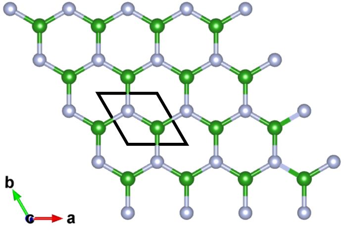
(a) h-BN

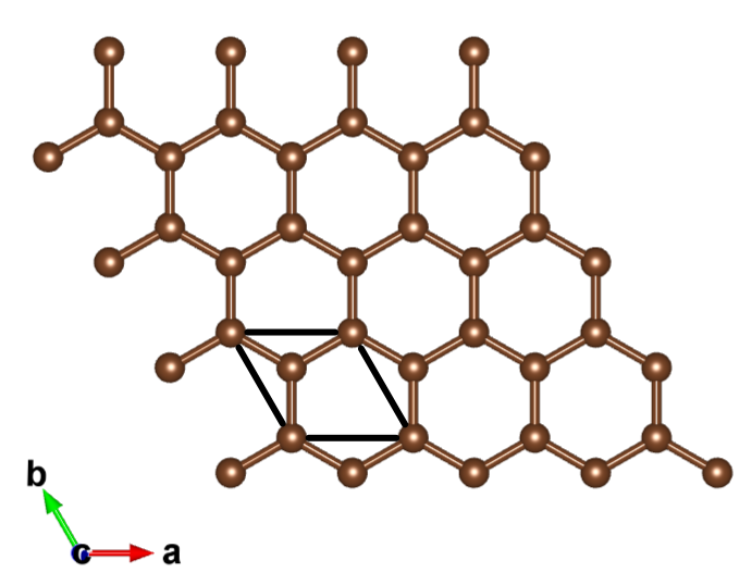
(b) Graphene

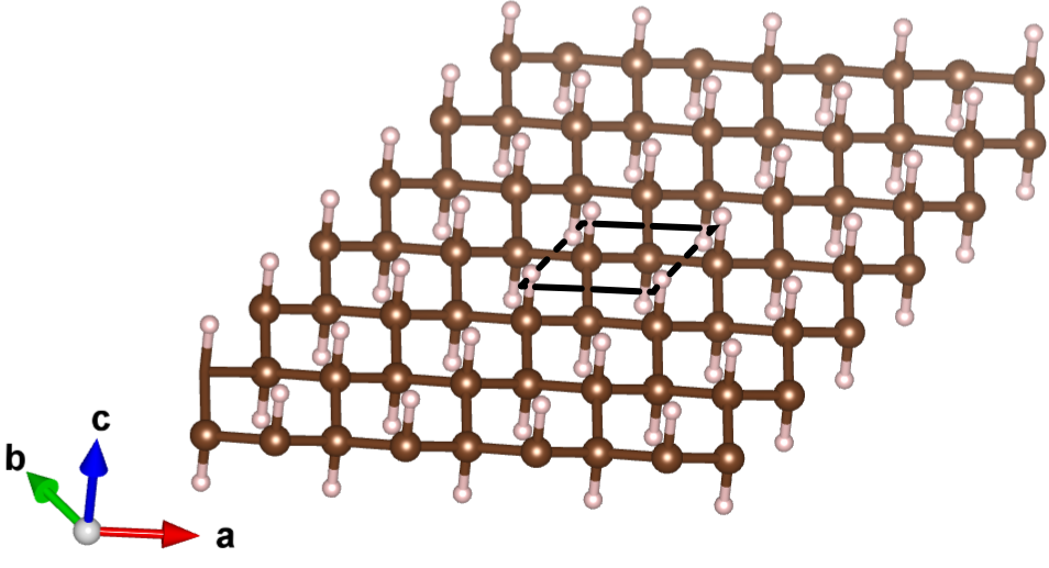
(c) Graphane

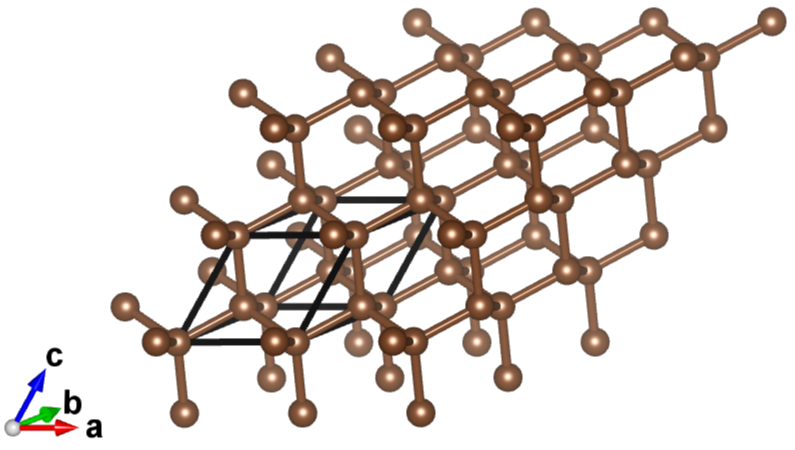
(d) Diamond

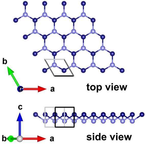
(e) Blue phosphorene

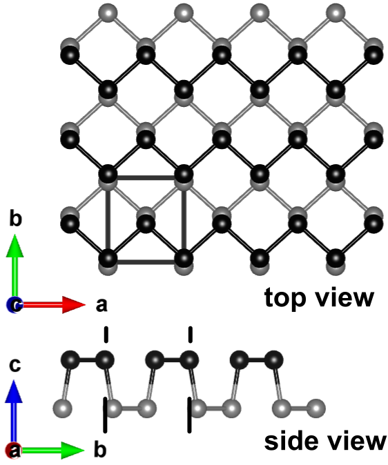
(f) Black phosphorene

Figure 1: Crystal structures of the compounds studied in this work.

I Introduction

The direct conversion of a temperature gradient to electric voltage or vice versa is known as the thermoelectric effect. Although first rigorously defined following a series of discoveries in the mid 19^th century, it was not until the mid 20^th century that materials exhibiting interesting thermoelectric properties were sufficiently understood to enable targeted research. Today, anthropogenic waste heat contributes significantly to climate change and for economic, as well as environmental reasons, creates a strong imperative to develop new thermoelectric materials.Tan et al. (2016) One feature of new materials often being exploited for potential thermoelectric applications is their anisotropy. Indeed, among the currently best performing materials are layered materials.Snyder and Toberer (2008) The low hanging fruits of science inevitably being picked first, such materials become ever more complex and contain an ever greater variety of chemical elements. The prediction of such materials’ fundamental thermoelectric properties using theoretical calculations prior to their synthesis can help experimentalists make specific choices in their target materials and, when such materials behave differently than predicted, such calculations can serve as a diagnostic tool.Yang et al. (2013)
The characteristic figure of merit for thermoelectric materials is typically denoted $ZT$, and defined as:

$$ZT=\frac{\sigma S^{2}T}{\kappa}$$ (1)

with $T$ the temperature (K), $\sigma$ the electrical resistivity (S m^-1), $S$ the “thermopower” or Seebeck coefficient (V K^-1) and $\kappa$ the thermal conductivity (W m^-1 K^-1). In crystalline materials the thermal conductivity is typically divided into contributions from electrons ($\kappa_{E}$) and phonons ($\kappa_{L}$), such that the total conductivity is the sum of both: $\kappa=\kappa_{E}+\kappa_{L}$.

According to the Boltzmann transport equation, the phonon (or lattice) conductivity along a certain crystallographic direction $\alpha$ can be further broken down toLi et al. (2014)

$$\kappa_{L}^{\alpha}=a(T)\sum_{j}\sum_{\bf q}f(f+1)v_{j\alpha}^{2}({\bf q})[\hbar\omega_{j}({\bf q})]^{2}\tau_{j}({\bf q}),$$ (2)

where $a(T)$ is a temperature dependent prefactor, $f$ denotes Bose-Einstein occupation factors, and $\omega_{j}({\bf q})$ and $\tau_{j}({\bf q})$ correspond respectively to the frequency and lifetime of a phonon in band $j$ at wave-vector ${\bf q}$. Finally, $v_{j\alpha}=\partial\omega_{j}/\partial q_{\alpha}$ stands for the phonon group velocity. While one needs to go beyond the harmonic approximation to obtain the phonon lifetimesTogo et al. (2015), both $\omega_{j}$ and $v_{j\alpha}$ are readily available from the phonon band structure (BS). An accurate description of the BS is therefore key to a reliable computation of the lattice conductivity, and by means of Eq. 1, also ZT.

First-principles determinations of the phonon BS are typically based on Density Functional Theory (DFT) which is the method of choice for systems with unit cells comprising several tens of atoms. Given that $ZT$ is inversely proportional to $\kappa$, recent attempts to increase thermoelectric effiency make use of nanostructured materials that feature extended structural defects Yamawaki et al. (2018) or complex unit cells Snyder and Toberer (2008) to suppress phonon conductivity. These are currently difficult to compute at the DFT level due to the high computational demands and empirical force fields like Tersoff Tersoff (1986) or Brenner Brenner (1990) potentials are used instead. Parameters for such empirical models are usually fitted to well understood crystals with simple geometry and might lack transferability to novel materials with unusual binding configurations. In addition, potentials for simulation cells with a larger number of different elements are scarce.

In the past years, density-functional theory based tight-binding (DFTB) Seifert et al. (1986); Porezag et al. (1995); Elstner et al. (1998) received a lot of attention, since it provides an intermediate level of theory between first-principles and empirical methods. In DFTB, the electronic DFT Hamiltonian is represented in a reduced atomic orbital basis and numerically evaluated at a reference density obtained from atomic DFT calculations. Differences between this reference density and the true electronic density are accounted for by means of a Taylor-like expansion. In order to compute total energies, additional pair potentials (the so-called repulsive potentials) are introduced and fitted to reproduce the DFT total energy. DFTB has the advantage of a firm foundation in DFT, while being three orders of magnitude faster than its parental method.

While there are a couple of investigations that analyze the accuracy of DFTB vibrational frequencies for finite molecular systems,Elstner (1998); Krüger et al. (2005); Gaus et al. (2013) phonon BS have never been systematically studied. The goal of this article is to provide a benchmark for DFTB and compare to available DFT results. Although accurate phonon BS are required in a variety of fields (e.g., in the interpretation of Raman and infrared spectra or phase transitions), we discuss the results with a particular emphasis on possible applications in thermoelectricity. This is reflected in the selection of investigated compounds, which are mostly (layered) 2D materials. Besides the large availability of phonon BS reference calculations for these now well-studied systems, this is also motivated by the predicted high figure of merit of such low-dimensional systems.Hicks and Dresselhaus (1993a, b) To be specific, we investigate h-BN and a selection of carbon based materials (graphene, graphane and diamond), with the aspiration of developing a framework for the emerging field of polymer-based thermoelectricity.Russ et al. (2016) Two allotropes of phosphorene were also studied to assess the possibilities of going beyond second row elements. In particular, we interfaced the DFTB+ Aradi et al. (2007) implementation of the DFTB method with the phonopyTogo and Tanaka (2015) code and apply a general phenomenological approach to compare a descriptor value for thermoelectricity with earlier experimental measurements and theoretical work.

Table 1: Slater-Koster sets used in this study. Hyphened elements in the second row correspond to subsets for which Slater-Koster files for all element pairs are available. The fifth row lists the targets: total energies ($E_{\text{tot}}$), orbital energies ($\epsilon_{i}$), geometries (F) and vibrational frequencies ($\omega$) that were aimed at during the fitting procedure.

SK set	Elements	DFTB level	Reference systems	Targets	Ref.
mio-1-1	O-N-C-H-S-P	2${}^{\text{nd}}$ order	molecules	$E_{\text{tot}}$, F, $\omega$	[Elstner et al., 1998]
pbc-0-3	Si-F-O-N-C-H, Fe	2${}^{\text{nd}}$ order	solids	N/A	N/A
matsci-0-3	Al-O-H, Al-Si-O-H, Cu-Si-Al-Na-O-H,	2${}^{\text{nd}}$ order	molecules	$\epsilon_{i}$, F	[Lukose et al., 2010]
	Ti-P-O-N-C-H, O-N-C-B-H, Al-O-C-H,
	Si-P-N-O-C-H
3ob-3-1	Br-C-Ca-Cl-F-H-I-K-Mg-N-Na-O-P-S-Zn	3${}^{\text{rd}}$ order	molecules	$E_{\text{tot}}$, F	[Gaus et al., 2012]
3ob:freq-1-2	C-C, C-N, C-O	3${}^{\text{rd}}$ order	molecules	$E_{\text{tot}}$, F, $\omega$	[Gaus et al., 2012]
borg-0-1	B-N	2${}^{\text{nd}}$ order	molecules	$E_{\text{tot}}$, F, $\omega$	[Grundkötter-Stock et al., 2012]

II Computational Details

II.1 DFTB calculations

DFTB calculations were performed with version 1.2 and 1.3 of the DFTB+ code.Aradi et al. (2007) The geometry optimzations were carried out using a charge tolerance of $10^{-6}$ in the self-consistent cycle and a maximum force component of $10^{-6}$ a.u.. Apart from carbon in the diamond structure, all other compounds in this study were treated as monolayers (and hence purely 2D materials) by imposing a unit cell dimension of 20 Å  perpendicular to the layer. We confirmed that this leads to neglible inter-sheet interactions. This choice was made to allow for a direct comparison to previous computational studies which often discuss monolayer dispersion relations. Moreover, any complication due to an insufficient treatment of the Van der Waals interaction between layers is avoided. All structures were then optimized by constraining the Bravais lattice to the experimental one and allowing the lattice constants and basis atoms to relax freely, starting in each case from the known crystal structure. Brillouin Zone (BZ) integrations were carried out using (16 $\times$ 16 $\times$ 1) Monkhorst-Pack (MP) k-point meshes.

In order to perform DFTB calculations, so-called Slater-Koster files are required for each element pair in the simulation cell. These contain tabulated Hamiltonian and overlap matrix elements, as well as the already mentioned repulsive potentials. The web repository www.dftb.org provides a source of currently available Slater-Koster sets, which have been generated by the DFTB community. Such sets generally differ in the actual basis set used to evaluate the DFT Hamiltonian, the highest order of the Taylor-like expansion around the reference density, and the reference systems used to create the repulsive potentials.Elstner and Seifert (2014) In addition, different groups place more emphasis on the accuracy of certain properties, like total energies, forces or vibrational modes in the fitting process.Gaus et al. (2011); Oliveira et al. (2015) Table 1 lists the Slater-Koster sets used in this study and provides additional information on their generation. Most sets were generated for molecular structures and without considering vibrations explicitly during the parameter generation, the set 3ob:freq-1-2 being a notable exception. The present study therefore provides a firm test to investigate the transferability of DFTB as a method, but also the transferability of specific Slater-Koster sets currently used.

II.2 Phonon-dispersion relations

DFTB+ has been interfaced to the phonopy code,Togo and Tanaka (2015) which provides a suitable framework to compute phonon BS by the supercell method (also often referred to as direct method). The new interface is available in phonopy version 2.1.2. Based on the primitive unit cell, phonopy creates several supercells with slightly displaced atoms. In a second step, DFTB+ single-point calculations are performed on these structures to compute the atomic forces. These are then collected by phonopy to evaluate the force constants by numerical differentiation and build the dynamical matrix, which yields the phonon BS through diagonalization.

Converged results were obtained by taking the supercell dimension to be (14 $\times$ 14 $\times$ 1) for graphene and graphane, (16 $\times$ 16 $\times$ 1) for h-BN and blue phosphorous, (8 $\times$ 8 $\times$ 1) for black phosphorous and finally (6 $\times$ 6 $\times$ 6) for diamond. For all supercells, the DFTB single-point calculations were carried out at the $\Gamma$-point.

II.3 Choice of reference

In order to assess the accuracy of the DFTB phonon-dispersions a reliable reference needs to be defined. The natural choice would be experimental data. Since measurements are not always performed at low-temperature conditions and include anharmonic effects, a direct comparison to 0 K computations in the harmonic approximation is not straightforward. For the 2D systems in the present study an additional complication arises: several compounds have not yet been synthesized as freestanding monolayers. This influences the band spectra through interlayer coupling and more importantly through interactions with the substrate. Hence, we chose first-principles DFT calculations as reference.

For molecular vibrations DFT has been extensively benchmarked in the chemistry community.Johnson et al. (1993); Rauhut and Pulay (1995); Finley and Stephens (1995); Hertwig and Koch (1995) The hybrid B3LYP and semi-local BLYP exchange-correlation functionals have emerged as reliable models with average errors of only 20-30 cm^-1 when appropriate scale factors are introduced.Scott and Radom (1996) Systematic benchmarks for the solid state are much scarcer. Previous studiesBaroni et al. (2001); Hummer et al. (2009); He et al. (2014) found a strong dependence of the results on the employed lattice constant. As an example, the LDA functional provided excellent results when the same level of theory was used to optimize the structure, but underestimated phonon modes at the experimental lattice constant.Hummer et al. (2009) Given the known tendency of LDA to underestimate cell volumes, this result can be understood as fortious error compensation. We finally decided to take the Perdew-Burke-ErnzerhofPerdew et al. (1996) gradient-corrected functional as reference level of theory, mainly because of the large body of available literature data and the good agreement with experiment (at the experimental volume) found in Ref. [Hummer et al., 2009]. For graphane no PBE literature data exists, and we performed or own calculations using Density-Functional Perturbation Theory as implemented in the Quantum Espresso suite of programs.Giannozzi et al. (2017) The corresponding computational parameters are given in the Supplemental Material.Sup

Table 2: Lattice parameters of the studied materials at different levels of theory in units of Å.

h-BN	LDA	PBE	HSE	matsci-0-3	borg-0-1	Tersoff	empirical	Expt.
$a$	2.494a	2.515b	2.510c	2.550	2.547	2.498d	2.505e	2.506f
Diamond	PBE	matsci-0-3	pbc-0-3	mio-1-1	3ob-3-1	3ob:freq-1-2	Expt.
$a$	3.574g	3.583	3.562	3.558	3.600	3.615	3.567h
Graphene
$a$	2.461i	2.467	2.472	2.471	2.474	2.491	2.46j
Graphane
$a$	2.540k	2.541	2.517	2.515	2.547	2.560	2.42l
Blue phosphorous	PBE	matsci-0-3	mio-1-1	3ob-3-1	Expt.
$a$	3.326m	3.545	3.467	3.426	3.28n
Black phosphorous
$a$	N/A	3.490	3.484	3.430	3.314o
$b$	N/A	4.375	4.368	4.300	4.376o

^a From Ref. [Wirtz et al., 2003]; ^b from Ref. [Mann et al., 2017]; ^c from Ref. [Cai et al., 2017]; ^d from Ref. [Anees et al., 2016a]; ^e from Ref. [Michel and Verberck, 2011a]; ^f from Ref. [Bosak et al., 2006]; ^g from Ref. [Hummer et al., 2009]; ^h from Ref. [Warren et al., 1967]; ⁱ from Ref. [Mounet and Marzari, 2005]; ^j from Ref. [Yazyev and Louie, 2010]; ^k current work; ^l from Ref. [Elias et al., 2009]; ^m from Ref. [Sun et al., 2016]; ⁿ from Ref. [Zhang et al., 2016]; ^o from Ref. [Brown and Rundqvist, 1965]

II.4 Harmonic descriptor

Several measures to quantify the accuracy of DFTB phonon-dispersion relations with respect to the reference could in principle be imagined. One possibility is to compare mode frequencies at special points in the BZ. One could also integrate the difference between DFTB and reference along full bands. Since we are interested in applications of DFTB in thermoelectricity, we define instead the following harmonic descriptor for each band $j$:

$$D_{j}=\int_{\mathcal{C}}\bar{v}_{j}^{2}({\bf q})[\hbar\omega_{j}({\bf q})]^{2}\,dq,$$ (3)

where the integral is evaluated along the high-symmetry lines in the BZ for which the BS is computed. The term $\bar{v}$ is the group velocity along this line. This measure is motivated by a comparison with Eq. 2 for the thermal conductivity. The descriptor $D_{j}$ incorporates the quantities entering the thermal conductivity that can be computed already in the harmonic approximation. Typically, optical phonons contribute less than acoustic modes to the thermal conductivity although their phonon frequencies are higher. This is due to a smaller curvature of the optical bands and hence smaller group velocity, an effect that is taken into account by the proposed descriptor.

To determine this descriptor also for the literature data, we first digitalized the corresponding band structures in the original articles using WebPlotDigitizer v. 4.1.Rohatgi (2018) Further, the data points were interpolated by cubic splines using the routines available in the SciPy Python library.Jones et al. (01) The spline representation also gives direct access to the band derivative. This allowed for a determination of the group velocities in all cases and gave good agreement with analytical group velocities computed directly by phonopy. Eq. 3 was finally evaluated by numerical integration using the trapezoidal rule with 5000 integration points between any two special points in the BZ.

Two measures for the discrepancy between the descriptor value at a certain level of theory and the reference (in our case DFT with the PBE functional) were chosen. First, a mean relative error was determined by the deviation of the descriptor value for each band from the corresponding reference values:

$$\text{MRE}={\frac{{\sum_{j=1}^{N}{\big{(}D_{j}-D^{\text{ref}}_{j}\big{)}}}}{{\sum_{j=1}^{N}{D^{\text{ref}}_{j}}}}},$$ (4)

where the sum is either over all bands or the subsets of acoustic and optical bands. A mean absolute relative error was applied in parallel, less sensitive to error cancellations:

$$\text{MARE}=\frac{\sum_{j=1}^{N}{\sqrt{\big{(}D_{j}-D^{\text{ref}}_{j}\big{)}^{2}}}}{\sum_{j=1}^{N}D^{\text{ref}}_{j}}.$$ (5)

III Results and Discussion

III.1 Structural properties

The structures and unit cells of the studied materials are depicted in Fig. 1. Here, h-BN, diamond and graphene are already well known. Monolayer graphaneSluiter and Kawazoe (2003), also termed hydrogenated graphene, is a hexagonal structure with two carbon and two hydrogen atoms in the unit cell. In the most stable chair configuration that is studied here, the hydrogens are alternately adsorbed above and below the graphene sheet.Sahin et al. (2015) Blue phosphorous is likewise a hexagonal structure that resembles graphene when viewed upon perpendicular to the sheet, but is non-planar. This first theoretically predicted allotrope Zhu and Tománek (2014) was later successfully synthesized as single layer material.Zhang et al. (2016) Single layer black phosphorous,Liu et al. (2014) also known as phosphorene, features an anisotropic structure with two lattice vectors of different length (see Fig. 1).

Table 2 summarizes the relevant lattice parameters obtained at the DFTB level using different Slater-Koster sets, as well as DFT and experimental literature data. For h-BN the largest body of reference data is available. Here we also included results from classical MD simulations using a Tersoff potential,Anees et al. (2016b) and an empirical force constant model.Michel and Verberck (2011a) Note that due to the limited availability of DFTB Slater-Koster files for certain elements, not all systems could be consistently studied with the same sets, matsci-0-3 being an exception.

For h-BN all considered methods agree with each other and differ from the experimental values by less than 2%. For the carbon based materials, pbc-0-3 and mio-1-1 yield nearly identical structures. The set 3ob:freq-1-2 tends to overestimate lattice constants. The largest deviation is found for graphane with an error of 6%, although the experimental value may be questioned in this case. It should be noted that all methods predict an increase of the lattice constant going from graphene to graphane, contrary to the experimental results. The phosphor compounds pose larger problems to DFTB. The matsci-0-3 set overestimates lattice parameters by 8% in the case of blue phosphorous and 5% for black phosphorous. The sets mio-1-1 and 3ob-3-1 likewise overestimate, but to a smaller degree.

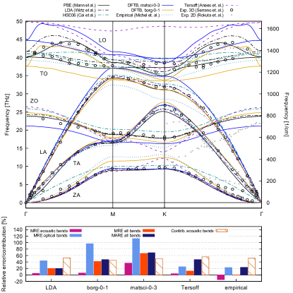
Figure 2: (Top) Single layer h-BN phonon dispersion. PBE results from Ref. [Mann et al., 2017], HSE06 (Ref. [Cai et al., 2017]), LDA (Ref. [Wirtz et al., 2003]), Tersoff potential (Ref. [Anees et al., 2016a]), empirical force field (Ref. [Michel and Verberck, 2011b]). The latter and also the HSE06 results are computed at the experimental geometry, all others use the lattice constant given by the respective method. Experimental results on 2D-h-BN@Ni(111) from Ref. [Serrano et al., 2007] and 3D-h-BN from Ref. [Serrano et al., 2007]. (Bottom) h-BN descriptor errors with respect to PBE for the acoustic, optical and the total number of bands. The relative contribution of the acoustic bands to the total descriptor value is likewise given.

III.2 Phonon band structures

Table 3: Descriptor values for h-BN. Mean relative error (Eq. 4) with repect to the PBE reference values for the descriptor of individual bands in h-BN. respectively. ”contr.” denotes the percentage contribution of the particular band to the total descriptor value. All values are expressed in %. To guide the eye, color markers indicate deviations $<$10 % (green), to 20% (yellow), to 50% (orange), 100% (red), 200% (purple) and $>$200% (black).

	LDA			borg-0-1			matsci-0-3			Tersoff			empirical
band		error	contr.		error	contr.		error	contr.		error	contr.		error	contr.
ZA	${\color[rgb]{1,1,0}\blacksquare}$	11.8	0.3	${\color[rgb]{0,0,0}\blacksquare}$	206.0	0.8	${\color[rgb]{1,1,0}\blacksquare}$	12.2	0.2	${\color[rgb]{0.65,0.0,0.65}\blacksquare}$	153.6	0.8	${\color[rgb]{0,0,0}\blacksquare}$	302.0	1.4
TA	${\color[rgb]{0,1,0}\blacksquare}$	4.0	12.1	${\color[rgb]{1.0,0.5,0.0}\blacksquare}$	40.3	13.8	${\color[rgb]{1.0,0.5,0.0}\blacksquare}$	29.0	10.8	${\color[rgb]{0,1,0}\blacksquare}$	1.9	12.7	${\color[rgb]{1,1,0}\blacksquare}$	12.5	15.7
LA	${\color[rgb]{0,1,0}\blacksquare}$	4.9	40.3	${\color[rgb]{0,1,0}\blacksquare}$	-6.2	30.6	${\color[rgb]{1.0,0.5,0.0}\blacksquare}$	39.0	38.6	${\color[rgb]{0,1,0}\blacksquare}$	2.9	42.4	${\color[rgb]{1.0,0.5,0.0}\blacksquare}$	-25.2	34.5
ZO	${\color[rgb]{1,1,0}\blacksquare}$	19.0	2.2	${\color[rgb]{1,0,0}\blacksquare}$	75.3	2.7	${\color[rgb]{1.0,0.5,0.0}\blacksquare}$	-45.5	0.7	${\color[rgb]{0,0,0}\blacksquare}$	230.0	6.5	${\color[rgb]{1,0,0}\blacksquare}$	76.2	3.9
TO	${\color[rgb]{1,0,0}\blacksquare}$	52.7	21.8	${\color[rgb]{0.65,0.0,0.65}\blacksquare}$	121.6	26.9	${\color[rgb]{0.65,0.0,0.65}\blacksquare}$	156.6	26.5	${\color[rgb]{0.65,0.0,0.65}\blacksquare}$	130.7	35.3	${\color[rgb]{1.0,0.5,0.0}\blacksquare}$	28.4	22.0
LO	${\color[rgb]{1.0,0.5,0.0}\blacksquare}$	38.6	23.2	${\color[rgb]{1,0,0}\blacksquare}$	77.4	25.2	${\color[rgb]{1,0,0}\blacksquare}$	92.0	23.2	${\color[rgb]{1,0,0}\blacksquare}$	-87.5	2.2	${\color[rgb]{1,1,0}\blacksquare}$	11.7	22.4

h-BN In Fig. 2, experimentally and computationally determined phonon band spectra reported in the literature for h-BN are visualized with our results. As usual, acoustic (optical) longitudinal and transverse modes are denoted as LA (LO) and TA (TO), respectively. In 2D materials, the flexural modes with atomic displacements perpendicular to the sheet are further labeled as ZO and ZA. One can see that the closed, grey symbols representing experimental results for 2D-h-BN are not reproduced by the different computational approaches, that are closer to the open symbols, representing 3D-h-BN. In practice, 2D-h-BN corrugates unpredictably and has to be suspended on a surface to be subjected to analysis.Serrano et al. (2007) This means that the experimental 3D-h-BN phonon band spectrum is probably closer to what an idealized experimental 2D-h-BN phonon band spectrum looks like than that of any practical h-BN monolayer. Although 3D-h-BN has four atoms in the unit cell and hence 12 bands are expected in the BS, the weak inter-layer interaction leads to two sets of essentially degenerate bands. As seen in Fig. 2, larger differences occur only close to the $\Gamma$-point for the ZA modes and reveal the 3D nature of the material.

Discussing first the DFT results, we find that PBE provides an excellent overall agreement with the experimental data by Serrano et al.Serrano et al. (2007) LDA provides the right dispersion throughout the BZ but overestimates the optical bands. This is opposite to the typical underestimation given by LDA for other materials.Hummer et al. (2009); He et al. (2014) The HSE results by CaiCai et al. (2017) do not qualitatively reproduce the phonon band spectrum for the ZA band. The flexural branch should exhibit a quadratic dispersion as discussed by Carrete et al.Carrete et al. (2016) Reasonable agreement with experiment is found for the DFTB Slater-Koster sets borg-0-1 and matsci-0-3 for the acoustical bands. Both show an accurate dispersion for the ZA branch. In fact, the numerical efficiency of DFTB permits to assess rather larger supercells and converge also long-range interactions that are important for finer details of the BS. As another example, h-BN features a maximum of the LO branch away from the $\Gamma$-point. This overbending is seen in all DFT and DFTB calculations and due to fifth-neighbour interactions.Michel and Verberck (2009) The optical bands of matsci-0-3 are not satisfactory: the LO and TA branches are overestimated by around 150 cm^-1 at the $\Gamma$-point, and at the same time the ZO branch is underestimated by roughly 100 cm^-1.

It should be noted that the DFTB approaches feature a second maximum in the paths $\Gamma\to$ M and K $\to\Gamma$, which is not seen in the PBE data or the experimental results. We verified that this feature is due to long-range Coulomb interactions in this weakly screened material. DFTB zeroth-order simulations, in which there is by construction no long-range charge-charge interaction, do not show this behaviour. We believe that the second maximum arises due to an incomplete treatment of these long-range interactions and could be overcome by a proper treatment of the nonanalytical part of the dynamical matrix.Wang et al. (2010) Unfortunately, the required Born charges and dielectric tensors are not yet implemented in DFTB+, such that we could not correct the BS at this point. The mentioned artefact concerns only the optical bands of polar materials in the limit $\Gamma\to$ 0 and is not expected to influence our general conclusions.

Turning finally to the empirical approaches, we find an overall good agreement with experiment for the results of Michel et al. Michel and Verberck (2009), while the dispersion of the optical bands is clearly wrong and largely overestimated for the Tersoff potential.

In order to see how these general trends might influence the lattice conductivity we now analyze the harmonic descriptor introduced in Sec. II.4. The PBE phonon band structure as determined using by Mann et al.Mann et al. (2017) was chosen as the reference to which the other methods were compared. Applying the descriptor yields the numerical values in Table 3 which are depicted in condensed form also in Fig. 2 bottom.

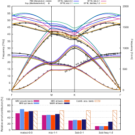
(a) Graphene

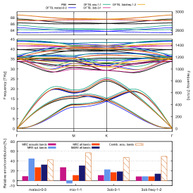
(b) Graphane

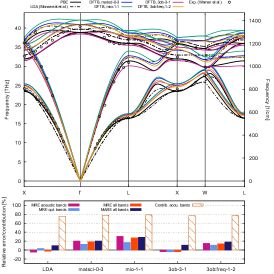
(c) Diamond

Figure 3: Phonon dispersion of carbon-based compounds. a) Graphene: PBE results from Ref. [Mounet and Marzari, 2005], for the experimental results see Ref. [Monteverde et al., 2015] and references therein; b) Graphane: PBE results from our work, no experimental results available; c) Diamond: PBE results at the experimental lattice constant from Ref. [Hummer et al., 2009], experimental results in Ref. [Monteverde et al., 2015]. If not mentioned otherwise, all calculations were performed at the optimized lattice parameter of the respective method. Bottom of each graph: descriptor errors and relative contribution of acoustic bands.

A crucial feature clear from Table 3 is that the apparent success of a method can be highly sensitive to certain spectral features, while being insensitive to others. The LA band, for example, alone accounts for $\sim 40\%$ of the total value. Although the difference in frequency of the LA band predicted by PBE and matsci-0-3 at the M-point - where that difference is highest - is less than $10\%$, the sensitivity of the descriptor is such that this translates in a +39% deviation in descriptor value for that band. Similarly, the Tersoff potential fails to describe either of the three optical bands in a qualitatively correct fashion; however, the LA and TA bands computed using the Tersoff potential faithfully follow the PBE, and experimental values. For this reason alone, its descriptor values are better than those of matsci-0-3, that reproduces the general trends predicted by PBE and experiment. The empirical model performs surprisingly well, although there are large discrepancies for the descriptor value of the ZA band. Since the flexural mode contributes only very little ($\sim 1\%$) to the total descriptor value, a rather small total error arises. As expected from the general earlier discussion, LDA performs well for the acoustic bands but overestimates the descriptor for the optical bands. The overall MARE of around 20 % is still the lowest of all tested methods.

Carbon-based compounds In Fig. 3 the results for the carbon compounds are shown. A large number of Slater-Koster sets do include carbon and hence a broader comparison is possible for this material class. Note that mio-1-1 and pbc-0-3 provided very similar BS and hence only mio-1-1 results are discussed in the following. We start the discussion with diamond, the only 3D crystal we considered. PBE follows the experimental phonon dispersion accurately. Also, all the DFTB models provide correct phonon dispersions for the acoustic bands, albeit slightly overestimated. The optical bands are also overestimated by around 100 cm^-1, with 3ob:freq-1-2 giving the smallest error. In total, the DFTB description of diamond is satisfactory. For graphene the acoustic bands are well reproduced, but the optical bands are displaced to higher frequencies by slightly over 200 cm^-1 for both pbc-0-3 and matsci-0-3. In contrast, 3ob:freq-1-2 yields very accurate BS as found already in an earlier study by Huang et al. Kuang et al. (2015). Graphane with its additional bands due to C-H stretch vibrations provides a harder challenge. Compared to the PBE reference (own calculations), these bands in the 2700 cm^-1 to 3000 cm^-1 range are either strongly overestimated (3ob-3-1, 3ob:freq-1-2) or underestimated (matsci-0-3, mio-1-1) by all DFTB models, while the optical C-C bands are generally overestimated. Again, 3ob:freq-1-2 yields the closest match to the reference.

This is also seen by considering the harmonic descriptor (Fig. 3 bottom), which consistently shows the lowest errors for 3ob:freq-1-2 with less than 30 % in all cases. Matsci-0-3 and mio-1-1 are less reliable with errors up to 60 % in the case of graphene. Considering the sets 3ob-3-1 and 3ob:freq-1-2, we find that 3^rd order DFTB leads generally to an improved description compared to 2^nd order DFTB, although the major improvement is seen for 3ob:freq-1-2 which was optimized for frequencies (see Table 1).

Comparing the overall results for graphane and graphene, the larger errors for the latter material are counter-intuitive. One would think that due to the structural similarity of both materials the descriptor errors should also be similar, with graphene having at most lower errors due the absence of C-H bands. The reason for this unexpected behaviour is related to the acoustic bands which range up to 1500 cm^-1 in the case of graphene, but only up to 800 cm^-1 for graphane. This leads to a smaller contribution of the LA and TA bands to the total graphane descriptor. In addition, the errors of both bands are likewise smaller for graphane. Another observation is related to the set mio-1-1, which shows a negative MRE for the optical bands in graphane. This can be traced back to the first optical band which contributes the most to the descriptor of the optical subset. Though mio-1-1 overestimates the frequencies of this band along the full path, the curvature is much smaller than the PBE reference, resulting in a smaller descriptor value. This non-uniform error in optical vs. acoustic bands as well as C-C vs. C-H vibrations (see above) leads to a rather small MRE for mio-1-1. Such an error compensation will also be present in the computation of the final lattice conductivities, but is clearly system dependent and not desireable.

The harmonic descriptor also allows to estimate the relative importance of optical and acoustic bands to the thermal conductivity. While the optical bands contribute only $\approx$ 20 % for diamond, this ratio increases to $\approx$ 40-50 % for graphene and graphane. This highlights the necessity for a proper description of all modes especially for complex unit cells with a larger number of optical bands.

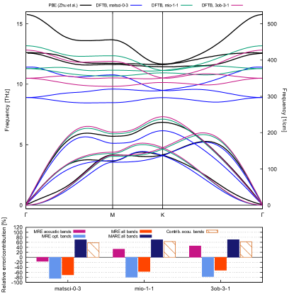
(a) Blue phosphorene

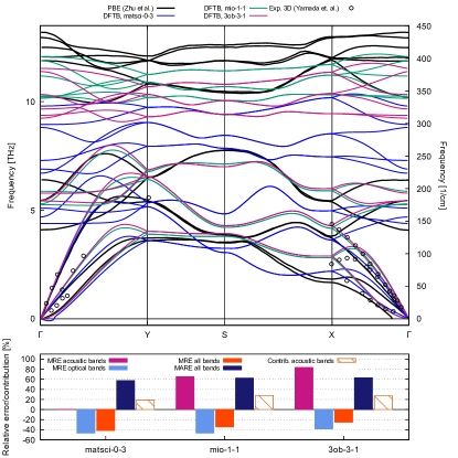
(b) Black phosphorene

Figure 4: Phonon dispersion of 2D phosphorus allotropes. For the PBE values, see Ref. [Sun et al., 2016], optimized lattice parameter. For the experimental values of black phosphorus, see Refs. [Yamada et al., 1984].

2D allotropes of phosphorus In DFTB one usually employs a minimal basis, taking only those atomic orbitals into account that are occupied in the respective atom. For second row elements, like sulfur or phosphorous, this approach leads to unsatisfactory results because of the hypervalent nature of bonding in some molecules.Niehaus et al. (2001) As a result, d-orbitals on the second row atom are typically included in the basis set to improve the results. It is therefore interesting to see how well DFTB performs for crystalline materials involving phosphorous.

In Fig. 4 the results for two allotropes of 2D-phosphorus, black and blue phosphorene, are depicted. Little is known about the experimental phonon band spectrum of black phosphorus, but the results for blue phosphorene (for which a comparison to experiment is possible) indicate that PBE is again an accurate reference. We find for blue phosphorene that all DFTB models strongly underestimate the optical branch brobdingnagianly. This can be traced back to the significant overestimation of the lattice constant (Table 2). Matsci-0-3 which delivers the largest error in the crystal structure also underestimates the optical bands by the largest amount ($\approx$ 30 %). A similar picture is obtained for black phosphorene. Here, matsci-0-3 predicts a qualitatively wrong dispersion with a minimum at S for the optical band in the 150 cm^-1 to 300 cm^-1 range. The Slater-Koster sets 3ob-3-1 and mio-1-1 perform slightly better in this regard but also differ strongly from the reference even for the acoustic bands along the path from S to X.

It should also be mentioned that regions of negative dispersion are found for PBE on the path X to $\Gamma$ and for matsci-0-3 on the path $\Gamma$ to Y. The direct approach for computing the phonon band structure is generally very sensitive to the numerical accuracy of the atomic forces. For DFTB, we have verified that the results are converged with respect to k-Point sampling, supercell size and the self-consistent field. In fact, only the matsci-0-3 SK set shows the mentioned artefact and we speculate that lower numerical accuracy for the SK tables at long inter-atomic distance could be the origin.

In Fig. 4 bottom the numerical results of the descriptor study clearly show the added difficulty of moving down a row in the periodic table. The data indicates a strong underestimation of descriptor values for the optical bands in blue phosphorene. This is due to the reduced dispersion and lower frequency of these bands in DFTB. As an example, the highest PBE band has a width of 140 cm^-1, while mio-1-1 gives a width of only 60 cm^-1. This also leads to quite different estimates for the band contribution ratio. While PBE predicts a very strong contribution of optical bands to the lattice conductivity with nearly 80 %, the DFTB values are much lower with 40 %. Not surprisingly, the total error of the descriptor is the largest among all systems studied with 70 % on average. DFTB with third order corrections (3ob-3-1) is not significantly better than the other Slater-Koster sets studied. The special parameterization for frequencies (c.f. 3ob:freq-1-2) is not available for phosphorous and seems to be an important factor to reach high accuracy.

IV Conclusions

Summarizing the results of the previous sections, one can say that the various available Slater-Koster sets provide in most cases accurate crystal structures and also acceptable acoustic band dispersions. Optical bands are described less well and can be shifted by several hundred wavenumbers with respect to the reference, typically to higher frequencies. Given that the Slater-Koster sets were parameterized for molecular structures, the overall performance indicates a reasonable degree of transferabilty. We found also that the accuracy varies strongly for different Slater-Koster sets. The set 3ob:freq-1-2 clearly outperforms other available sets, but is clearly limited in the available element combinations. Judging its quality based on the harmonic descriptor, 3ob:freq-1-2 deviates from PBE by roughly 20 % (MARE) on average over the carbon based materials. For comparison, the LDA results differ also by 20 % from the reference for h-BN.

Not surprisingly, Slater-Koster sets which were created with molecular vibrational frequencies as one of the fitting targets perform the best. This would indicate that new sets covering further elements should always follow this strategy. Unfortunately, there is evidence that accurate energetics and vibrations are mutually exclusive targets. For applications in thermoelectricity this presents no real problem, since Slater-Koster sets created with a special emphasis on frequencies do also deliver accurate crystal structures (as we have shown) which is a prerequisite for proper lattice conductivities. Only in cases where two phases of the target material are energetically close, special care is warranted.

We conclude that the harmonic properties of 2D materials can be successfully computed using the DFTB method at a fraction of the computational cost of full DFT calculations. This opens possibilities to perform previously inaccessible phonon dispersion calculations on thermoelectric polymers and defect engineered layered materials. Whether phonon lifetimes from third-order force constants are also sufficiently accurate is currently under study in our laboratory.