Disentangling Options with Hellinger Distance Regularizer

Abstract

In reinforcement learning (RL), temporal abstraction still remains as an important and unsolved problem. The options framework provided clues to temporal abstraction in the RL, and the option-critic architecture elegantly solved the two problems of finding options and learning RL agents in an end-to-end manner. However, it is necessary to examine whether the options learned through this method play a mutually exclusive role. In this paper, we propose a Hellinger distance regularizer, a method for disentangling options. In addition, we will shed light on various indicators from the statistical point of view to compare with the options learned through the existing option-critic architecture.

1 Introduction

Hierarchical learning has been considered as a major challenge among AI researchers in imitating human beings. When solving a problem, human beings subdivide the problem to create each hierarchy and arrange it in a time sequence to unconsciously create an abstraction. For example, when we prepare dinner, we follow a series of complicated processes. The overall process of cooking the ingredients, cooking them along with the recipe and setting the food on the table includes detailed actions such as cutting and watering in detail. This process can be described as a temporal approach and is currently being addressed in the study of AI Minsky (1961); Fikes et al. (1972); Kuipers (1979); Korf (1983); Iba (1989); Drescher (1991); Dayan and Hinton (1993); Kaelbling (1993); Thrun and Schwartz (1995); Parr and Russell (1998); Dietterich (1998). Temporal abstraction in reinforcement learning (RL) is a concept that a temporally abstracted action is conceptualized to understand problems in a faster and efficient way by understanding problems hierarchically for efficient problem-solving.

However, how to implement temporal abstraction in RL is still an open question. The framework of options Sutton et al. (1999) provided a basis for solving the RL problem from the viewpoint of temporal abstraction through the semi-Markov Decision Process (sMDP) based on options. The options are defined as temporally extended courses of actions. Mann and Mannor (2014); Mann et al. (2015) showed that the model trained using the options converges faster than the model trained with the primitive actions. Bacon et al. (2017) then proposed an option-critic architecture. In this architecture, they extracted features from deep neural networks and combined the actor-critic architecture with the options framework. With this approach, they solved two combined problems that finding options based on data without prior knowledge and training the RL agent to maximize reward in an end-to-end manner. Later, Harb et al. (2017) devised a way to learn options that last a long time by giving the cost of terminating the options. In Harutyunyan et al. (2017), they proposed a solution to the problem of degrading performance due to the sub-optimal options by training the termination function in an off-policy manner.

In this paper, we are going to analyze the model based on the option-critic architecture in different two perspectives and propose a method to improve the problems. First, we will verify that the options learned from option-critic plays the role of sub-policy. We expect each option to play a different role. In the option-critic architecture, the number of options is set as a hyperparameter without prior knowledge of the environment. In the process of optimizing the objective function, the different learned options often follow a similar probability distribution Bacon et al. (2017). It is certain that this is not the direction we expect for the options framework, and we can expect that similar options will lead to inefficient learning.

Second, we will examine what options the agent learns from a variety of perspectives. The previous studies have focused on creating a model that guarantees high reward and fast convergence based on confidence in the options framework Vezhnevets et al. (2016); Bacon et al. (2017); Harb et al. (2017); Harutyunyan et al. (2017); Vezhnevets et al. (2017); Tessler et al. (2017); Smith et al. (2018). However, it is also meaningful to look at how the learning progresses as well as the performance.

The options can be represented as stochastic probability distributions of actions. So we will evaluate whether there is a significant difference between the learned options in terms of stochastic perspectives. First, we examine the probability distribution of each intra-option policy at the same state from the learned model. We then use statistical distance measures such as Kullback-Leibler divergence Kullback and Leibler (1951) and Hellinger distance Hellinger (1909), which is a kind of f-divergence Csiszár et al. (2004). Also, the state space learned by the network can be expressed as t-SNE Maaten and Hinton (2008) at the latent variable stage, and we will also check whether the options play different roles depending on how the different options are activated in the state space.

In order to overcome the problems of the existing option-critic architecture, we propose a way to induce the options to learn mutually exclusive roles. Our approach is based on the assumption that intra-option policies would be mutually exclusive if they learn different probability distributions. We considered various statistical distances, and used Hellinger distance as the regularizer that best matches our purpose. When we applied our method to Arcade Learning Environment (ALE) Bellemare et al. (2013) and MuJoCo Todorov et al. (2012) environment, we could verify that the agent disentangles the options better while maintaining performance.

To summarize, our contribution in this paper is as follows.

• Propose a method of Hellinger distance regularizer and show the possibility of distangling options in RL.

• Examine trained options by option-critic architecture and our methods in detail with diverse measures.

We will proceed this paper in the following order. First, we overview the reinforcement learning and options, the background of the problem we want to solve. And we investigate how we can measure the difference between options in terms of statistical distance. Based on this, we propose a method to disentangle the options, and we show that disentangling options is possible through our proposed method from various viewpoints by conducting experiments in ALE and MuJoCo environment.

2 Background

2.1 Reinforcement Learning

In this paper, we work with Markov Decision Processes (MDPs), which are tuples $\langle S,A,r,P,\\ \gamma\rangle$ consisting of a set of states $S$, a set of actions $A$, a transition function $P_{a}(s,s^{\prime})$, a reward function $r:R_{a}(s,s^{\prime})$, and a discount factor $\gamma$. A policy $\pi$ is a behavior function determined by $Pr(s_{t+1}=s^{\prime}|s_{t}=s,a_{t}=a)$ which indicates the probability of selecting an action in a given state. The value of a state $V^{\pi}(s)$ is defined as $V^{\pi}(s)=\mathbb{E}[\sum_{t=1}^{\infty}\gamma^{t}r_{t}]$ which indicates the expected sum of discounted rewards when following the policy $\pi$.

2.2 Options

The Options Framework Sutton et al. (1999) suggested the idea for learning temporal abstraction through an extension of a reinforcement learning framework based on semi-Markov decision process (sMDP). They used the term options, which include primitive actions as a special case. Any fixed set of options defines a discrete-time sMDP embedded within the original MDP. Options consist of three components: a policy $\pi:S\times A\xrightarrow{}[0,1]$, a termination condition $\beta:S\xrightarrow{}[0,1]$, and an initiation set $\mathbb{I}\subseteq S$. If an option is chosen, then actions are selected through $\pi$ until the termination term $\beta$ stochastically terminates an option. They also suggest policies over options $\mu:S\times O\xrightarrow{}[0,1]$ that selects an option $o\in O_{s_{t}}$ according to a probability distribution $\mu(s_{t},\cdot)$

Option-Critic Architecture Bacon et al. (2017) suggested an end-to-end algorithm on learning an option. They suggested the call-and-return option execution model, in which an agent picks option $\omega$ according to its policy over option $\pi_{\Omega}$, then follows the intra-option policy $\pi_{\omega}$ until termination $\beta_{\omega}$. The intra-option policy $\pi_{\omega,\theta}$ of an option $\omega$ is parameterized by $\theta$ and the termination function, $\beta_{\omega,\vartheta}$ of the option $\omega$ is parameterized by $\vartheta$. They proved both intra-option policy and termination function are differentiable with respect to their parameters $\theta$ and $\vartheta$ so that they can design a stochastic gradient descent algorithm for learning options. The option-value function is defined as:

$$Q_{\Omega}(s,\omega)=\sum_{a}\pi_{\omega,\theta}(a|s)Q_{U}(s,\omega,a)$$ (1)

where $Q_{U}:S\times\Omega\times A\xrightarrow{}\mathbb{R}$ is the value of executing an action in the context of state-option pair:

$$Q_{U}(s,\omega,a)=r(s,a)+\gamma\sum_{s^{\prime}}P(s^{\prime}|s,a)U(\omega,s^{\prime})$$ (2)

Here, $U(\omega,s^{\prime})$ is the option-value function upon arrival of option $\omega$ at state $s^{\prime}$ Sutton et al. (1999). In Harb et al. (2017), they suggested the deliberation cost function, which is essentially a negative reward that they give to the agent whenever it terminates an option.

$$\begin{split}U(\omega,s^{\prime})=&(1-\beta_{\omega,\vartheta}(s^{\prime}))Q_{\Omega}(s^{\prime},\omega)\\ &+\beta_{\omega,\vartheta}(s^{\prime})(V_{\Omega}(s^{\prime})-c)\end{split}$$ (3)

Eq. 3 explains the value function for an option-critic architecture. $c$ indicates the deliberation cost which acts like a regularizer presented in Bacon et al. (2017) but it takes a more significant role.

3 Distance between Options

In the options framework, the intra-option policy is expressed as a probability distribution over actions when a state is given. We believe the intra-option policy must show different probability distributions over actions in order to argue that each option plays a different role in RL. Therefore, it is necessary to measure the distance between probability distributions to see whether the options are mutually exclusive. In this section, we look at a way to measure the distance between probability distributions in terms of statistical distance.

Statistical distance Csiszár (1967) defines the difference of two probability distributions $P,Q$ by the following f-divergence.

$$D_{f}(P\|Q)=\sum_{x}Q(x)f\left(\frac{P(x)}{Q(x)}\right)$$ (4)

Here, $f(t)$ is a convex function defined for $t>0$ and $f(1)=0$ in Eq. 4 Csiszár et al. (2004). The f-divergence is 0 when the probability distributions $P$ and $Q$ are equal and non-negative due to convexity. There are various instances of f-divergence according to different choices of a function $f$, and we used Kullback-Leibler divergence and Hellinger distance to measure the difference in options.

Kullback-Leibler Divergence (KLD) Kullback and Leibler (1951) is a representative measure of the probability distributional difference, and the function $f$ of f-divergence is $f(t)=t\log t$. KLD is defined as follows when the probability distributions $P$ and $Q$ are discrete and continuous, respectively.

$$D_{KL}(P\|Q)=-\sum_{x}P(x)\log\left(\frac{Q(x)}{P(x)}\right)$$ (5)

$$D_{KL}(P\|Q)=-\int_{-\infty}^{\infty}p(x)\log\left(\frac{Q(x)}{P(x)}\right)dx$$ (6)

Since KLD follows the properties of the f-divergence, it is always non-negative and zero when the probability distributions $P$ and $Q$ are equal. But it is an asymmetric measure and the value $D_{KL}(P\|Q)$ is not equal to $D_{KL}(Q\|P)$. This is because KLD can be expressed as the difference in the amount of additional information needed to reconstruct the probability distribution $P$ with probability distribution $Q$ Cover and Thomas (2012). In order to complement the asymmetry of KLD, Lin (1991) proposed Jensen-Shannon divergence (JSD). However, we do not use JSD because it is impossible to calculate a closed form solution for the continuous probability distribution and we cannot apply it to the continuous action space we would experiment with.

Hellinger Distance (HD) Hellinger (1909) is the case where the function $f$ of f-divergence is $f(t)=1-\sqrt{t}$. And the discrete and continuous Hellinger distance of the probability distributions $P$ and $Q$ are defined as follows.

$$H(P,Q)=\frac{1}{\sqrt{2}}\sqrt{\sum_{i=1}^{k}(\sqrt{P_{i}}-\sqrt{Q_{i}})^{2}}$$ (8)

$$H(P,Q)=\sqrt{1-\int_{\infty}^{-\infty}\sqrt{P(x)Q(x)}dx}$$ (9)

In Eq. 8 $P$ and $Q$ are $k$-dimensional multivariate distributions. The HD can be interpreted as the L2-norm of the probability distributions. In addition, the HD is bounded to $[0,1]$, while having the property of f-divergence. The maximum distance of $H(P,Q)$ is achieved when the probability of $Q$ is zero for a set where the probability of $P$ is greater than 0, and vice versa.

4 Disentangling Options

4.1 Hellinger Distance Regularizer

We believe that the different options must play a different role in the same RL environment in order to be meaningful in terms of temporal abstraction. However, as we will check in the experiments of Section 5, the options learned in the option-critic architecture may play a similar role. We , therefore, propose a regularizer that can disentangle options from a statistical distance perspective. We will add the HD to the loss and use it as a regularizer. As we have seen in Section 3, the HD can be calculated as a closed differentiable form in both continuous and discrete probability distributions and has the desirable properties that it is non-negative and bounded in between 0 and 1.

On the other hand, the other candidate we looked at in Section 3 is possible to measure the difference in options, but it is not suitable as a regularizer. In the case of KLD, it is sometimes used as a regularizer to narrow the difference between distributions like in the case of Variational Autoencoder Kingma and Welling (2013). But it is not appropriate as a regularizer for our case, because it does not have an upper bound while we intend to widen the difference between distributions. If we use KLD as a regularizer, the value will diverge to infinity and fail to train the model.

We defined the HD regularizer (hd-regularizer) as follows:

$$L_{hd-reg}=\frac{1}{{}_{m}C_{2}}\sum_{P}\sum_{Q}H(P,Q),\quad P\neq Q$$ (10)

Here, ${}_{a}C_{b}$ is the number of $b$ combinations among $a$ choices and the hd-regularizer loss calculates the average of the Hellinger distances of two different options when there are $m$ options.

[OC] [OC+HD]

Figure 1: Histogram of intrinsic rewards by options learned from (a) option-critic architecture (OC) and (b) our hd-regularizer method (OC+HD) in MuJoCo Swimmer-v2. The horizontal axis is the corresponding reward. The distributions of different options in OC are largely overlapped. On the other hand, options in OC+HD focus on different area of intrinsic rewards.

$(\%)$ o0 o1 o2 o3 OC 0.75 2.37 55.62 41.25 OC+HD 5.75 59.87 9.12 25.25

Table 1: Option use rate of option-critic architecture(OC) and hd-regularizer method(OC+HD) in MuJoCo Swimmer-v2. Each column is an option label.

4.2 Disentangling Options and Controllability

We expect to add an hd-regularizer to the option-critic architecture to disentangle the intra-option policy that the option learns. We think that the expected utilization of disentangled options is in the controlling of an agent. The ultimate goal of RL is to create an agent that can perform like a human being or better, and the real world problems are more complex than the environments we are experimenting with. And in a complex environment, the reward to achieve must be more complex than that of a simple environment and be composed of multiple sub-rewards. We think it would be possible to control the agent in the desired direction if the options are disentangled and different options perform different functions focusing on different rewards, as we expected. It is possible to have control over an agent if the options are used differently, such as in a soccer match, where the coaches change aggressive or defensive tactics depending on the situation.

We try to check the feasibility of disentangling options and controllability based on experiments in environments with multiple rewards. When training an agent in the MuJoCo’s Swimmer-v2 environment, it has two implicit rewards whose combination makes up a total reward. Fig. 1 shows the histogram of both intrinsic rewards for each option learned by the option-critic architecture (OC) and our method which uses a hd-regularizer (OC+HD). In this figure, we have confirmed that when using our method, the options focus on different intrinsic rewards and we have interpreted it as feasibility for controllability. See Section 5.3 for more details.

5 Experiments

Through experiments, we will identify the problems with existing option-critic architectures and compare the aspects of our proposed hd-regularizer and the option-critic architecture in various ways. We conduct experiments in the Arcade Learning Environment (ALE) Bellemare et al. (2013) and MuJoCo Todorov et al. (2012) environment using the advantageous actor-critic (A2C) of Schulman et al. (2017) as the base algorithm. The network architecture and hyperparameters are also set equal to those of the base algorithm for each environment. With regard to the option-critic architecture, we followed the structure of Bacon et al. (2017). The number of options is fixed as 4 and the policy over option follows $\epsilon$-greedy policy with $\epsilon=0.01$ and the intra-option policy is trained by A2C method. We used RMSprop Tieleman and Hinton (2012) optimizer and updated the weight whenever 16 processes proceeded 5 steps. The loss function consists of the option-critic loss, the entropy regularizer, and the hd-regularizer. The option-critic loss consists of the policy gradient loss for the intra-option policy and value loss to estimate the option-value function, termination gradient loss and deliberation cost loss. We used an entropy regularizer to prevent intra-option policy from becoming deterministic too early and to encourage exploration Williams and Peng (1991). Finally, we added the hd-regularizer to the loss after hyperparameter tuning. In order to prevent the intra-option policy from becoming fully deterministic in the discrete action space environment due to the hd-regularizer, we clamped the minimum probability of action of the policy to $10^{-4}$. Details of the experimental setup are provided in the supplementary material.

5.1 Arcade Learning Environment

We experimented in the following six environments of Atari2600 provided by ALE with reference to Bacon et al. (2017); Harb et al. (2017): AmidarNoFrameskip-v4, AsterixNoFrameskip-v4, BreakoutNoFrameskip-v4, HeroNoFrameskip-v4, MsPacmanNoFrameskip-v4, and
SeaquestNoFrameskip-v4. Observation is a raw pixel image that stacked 4 frames as in Mnih et al. (2013). The network consists of 3 convolutional layers with ReLU as the activation function and 1 fully-connected layer with option-value function, termination function, and intra-option policy stacked. And we trained $10^{7}$ steps per experiment. In addition, we used a clipped reward, the sign of actual reward, to reduce the performance impact of rewards with different scales for each environment.

5.1.1 Reviewing Trained options

First, through experiments, we have confirmed that temporal abstraction through the framework of options is not always required for all RL problems. Table 3 is the average reward and standard deviation of five runs of experiments with different random seeds for each algorithm and Table 3 summarizes the option use rate for each environment in one of the five experiments. First, when comparing the results from a reward perspective, except for MsPacman, all three methods show similar performance.In the case of MsPacman, the performance of the option-critic architecture and our method, using the options framework, was better than the baseline. From this result, the temporal abstraction through options does not always seem to guarantee performance improvement, in terms of rewards.

Environment A2C OC OC+HD Amidar 346.81$\pm$91.75 318.63$\pm$51.73 305.85$\pm$32.55 Asterix 4412.80$\pm$1318.23 4321.50$\pm$1502.66 3985.70$\pm$584.01 Breakout 355.10$\pm$38.31 349.54$\pm$58.87 355.21$\pm$25.25 Hero 15834.35$\pm$3459.75 14713.78$\pm$2264.49 15229.56$\pm$2640.07 MsPacman 1361.18$\pm$384.06 1934.50$\pm$170.32 1910.96$\pm$344.30 Seaquest 1701.56$\pm$50.85 1687.52$\pm$49.64 1724.08$\pm$25.31

Table 2: Average reward and its standard deviation from Arcade Learning Environment experiments. We tested with advantageous actor-critic(A2C), option-critic architecture(OC) and hd-regularization method(OC+HD). Each experiment was performed 5 times per environment.

$($%$)$ OC OC+HD Environment o0 o1 o2 o3 o0 o1 o2 o3 Amidar 0.0 26.43 73.56 0.0 53.25 7.37 38.0 1.37 Asterix 0.35 0.14 99.51 0.0 56.25 0.0 43.75 0.0 Breakout 99.34 0.63 0.03 0.01 0.0 0.0 0.0 100 Hero 0.0 1.23 29.61 67.16 0.25 0.0 24.5 75.25 MsPacman 41.6 0.09 34.44 23.88 7.75 0.5 60.75 31.0 Seaquest 100 0.0 0.0 0.0 0.0 100 0.0 0.0

Table 3: Option use rate of option-critic architecture(OC) and hd-regularization method(OC+HD) in Arcade Learning Environment. Each column is an option label.

We can also verify that the options framework is not always required through the use of trained options. Table 3 summarizes the option use rate for each environment in one of our experiments. We can divide the environment into several groups. First, in Breakout and Seaquest, both the option-critic architecture and our method solves the problem using only one option. A possible explanation is that one option-value function would have an advantageous value for all states of the environment during $\epsilon$-greedy learning. In this case, the use of the options framework is not essential to solve RL problems. The remaining four environments, except Breakout and Seaquest, belong to the second group and have been trained to use a variety of options in both methods. The second group can be said to have meaningful learning through the options framework, so we will continue to focus on these environments.

[OC] [OC+HD]

Figure 2: t-SNE plot of option-critic architecture(OC) and hd-regularization method(OC+HD) in $Hero$. Each point represents a state and the color of the point is an option used in the state.

From Table 3, we can see that in Hero, both option-critic and our method use two major options, option2 and option3. Major options occupy more than 90 percent of the option usage, and minor options are rarely used. The state of two models can be examined in the latent variable space after convolutional layers and one fully-connected layer explained in Section 5.1. Fig. 2 is a representation of latent space with t-SNE Maaten and Hinton (2008), and both option-critic and our method appear to use options by disentangling states. If we look at this figure alone, it can be thought that both methods use the options well, but it does not if we look at the options in more detail.

Figure 3: Captured state images and intra-option policies of option-critic architecture(OC) and hd-regularization method(OC+HD) in Hero. The heatmap above and below center the captured environment image represents a probability distribution of intra-option policy. Rows and columns of the heatmap are options and available actions. And the color of the heatmap is the probability of performing an action. An activated option at state is marked as red shaded.

Fig. 3 represents the probability distribution of the intra-option policy of the options of both methods when encountering a similar state in $Hero$. Top row is the intra-option policy of the option-critic architecture and bottom-row is the intra-option policy of our method with the hd-regularizer. The row of each intra-option policy is an option, column means discrete action, and the probability is expressed in a heatmap. And the shaded part in the option label of each row means that the option is activated at that state. In Table 3, option2 and option3 are major options of the option-critic model. In Fig. 3, all states of the intra-option policy learned in option-critic follows a similar probability distribution of option2 and option3. Using an option that follows a similar distribution means that both options have the same function and have done unnecessary learning. On the other hand, most of the hd-regularizer methods have different intra-option policies in the states.

KLD HD Environment OC OC+HD OC OC+HD Amidar 1.22$\pm$0.56 6.85$\pm$1.71 0.43$\pm$0.07 0.90$\pm$0.08 Asterix 1.98$\pm$1.26 7.47$\pm$1.44 0.50$\pm$0.10 0.92$\pm$0.05 Breakout 2.78$\pm$2.57 6.61$\pm$2.87 0.53$\pm$0.18 0.85$\pm$0.85 Hero 2.97$\pm$2.02 7.21$\pm$1.36 0.52$\pm$0.05 0.93$\pm$0.04 MsPacman 10.64$\pm$5.45 7.37$\pm$1.16 0.78$\pm$0.11 0.91$\pm$0.07 Seaquest 0.50$\pm$0.33 7.09$\pm$2.05 0.29$\pm$0.08 0.93$\pm$0.05

Table 4: An average distance between options and its standard deviation from option-critic architecture(OC) and hd-regularization method(OC+HD) measured by KLD and HD in Arcade Learning Environment.

5.1.2 Analysis with Measures

Here, we compare the similarities of the learned options numerically through two measurement methods: kl-divergence and Hellinger distance discussed in Section 2. Table 4 is the average of the distance between options learned in each environment. In the case of KLD, the values obtained by hd-regularizer method are larger than option-critic architecture in all environments except Hero. And the HD has larger values in our method for all environments and the values are close to 1 which is the upper bound of the HD. That is, the distance between the intra-option policy distributions is further with the hd-regularizer method. From this, we can see that the options learned by applying the hd-regularizer are disentangled in terms of statistical distance than those learned by the option-critic architecture.

5.2 MuJoCo Environment

We also experimented for four environments of MuJoCo with reference to Smith et al. (2018):Hopper-v2, Walker2D-v2, HalfCheetah-v2 and Swimmer-v2. MuJoCo environment is based on continuous action space, so the environment setting is quite different from the previous setting. Observation is provided by MuJoCo environment as state space and stacked 4 frames similar to ALE setting. We conducted the network structure of Schulman et al. (2017) and Smith et al. (2018) with two hidden layers of 64 units with $tanh$ activation function for both value function and the policies. The intra-option policies were implemented as Gaussian distribution with hidden layers of mean and bias from the network. And we trained $2\times 10^{6}$ steps for MuJoCo environment.

5.2.1 Reviewing Trained Option

As we can see in Table 6, options work more effectively in the continuous action space than in the ALE. The result shows that the options are more effective than the environment with discrete actions by showing a slightly higher or almost equal result in the option-critic architecture than the A2C. It can be said that the number of option is one factor that determine the complexity of the environment. And the policies of the two methods using the options framework here have bigger capacity than that of baseline method, A2C, because they have additional parallerized intra-option policy networks. Therefore, we think a learning method using the options framework will work better in a complex environment. From Table 6, the complexity of a continuous action space seems to maximize the benefit of the action capacity of the option. Especially, when using the options framework, there is no big difference in the action space of Swimmer(2) and Hopper(3), but the action space is wider and the complexity is higher in the environment of HalfCheetah(6) and Walker2d(6), we can see that the regularizing effect using the options works effectively. This also applies to the assumption that the higher the complexity, the greater the effect of temporal abstraction.

We also confirmed that the option framework is not necessarily required in the MuJoCo environment. In Table 6, we compared option use rates in each MuJoCo environment. Like the ALE, we can divide the experimented four environments into two groups. The first group is Hopper and HalfCheetah environment which seem to be leaning towards one option-value function while learning with $\epsilon$-greedy. It tends to train a RL agent by using only one option in the option-critic architecture. In the case of using the hd-regularizer, the agent use more options in the Hopper. This means that our method encourages the agent to learn more validate options by disentangling temporally abstracted options.

Environment A2C OC OC+HD Hopper-v2 1299.3$\pm$685.11 1393.2$\pm$191.62 1377.7$\pm$255.72 Walker2d-v2 1226.8$\pm$805.98 1804.7$\pm$785.08 1664.1$\pm$374.32 HalfCheetah-v2 1421.6$\pm$133.81 1403.6$\pm$54.33 1773.1$\pm$551.18 Swimmer-v2 34.73$\pm$2.04 34.97$\pm$1.61 36.13$\pm$1.63

Table 5: Average reward and its standard deviation from MuJoCo Environment experiments. We tested with advantageous actor-critic(A2C), option-critic architecture(OC) and hd-regularization method(OC+HD). Each experiment was performed 5 times per environment.

$($%$)$ OC OC+HD Environment o0 o1 o2 o3 o0 o1 o2 o3 Hopper 100 0.0 0.0 0.0 0.12 50.75 31.75 17.37 Walker2d 4.12 12.75 3.75 79.37 10.75 10.25 75.12 3.88 HalfCheetah 0.0 100 0.0 0.0 0.0 100 0.0 0.0 Swimmer 88.37 11.5 0.12 0.0 5.00 85.25 3.62 6.12

Table 6: Option use rate of option-critic architecture(OC) and hd-regularization method(OC+HD) in MuJoCo Environment. Each column is an option label.

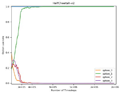
[OC] [OC+HD]

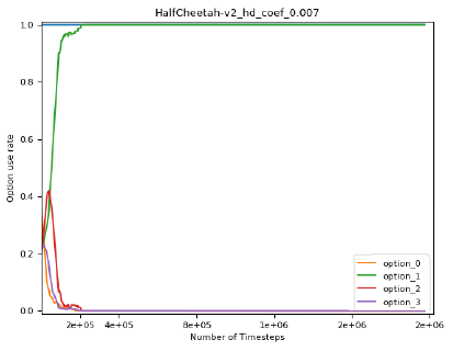
Figure 4: Training curves of option use rates for option-critic architecture(OC) and hd-regularization method(OC+HD) in $HalfCheetah$. The major option use rate of OC+HD converges to 100% faster than that of OC.

The unusual point is that in HalfCheetah environment, the final reward is higher than the A2C or option-critic method, although the proposed method concludes that it is much better to use only one option. Fig. 4 is a graph comparing the option use rates of the option-critic architecture method and the proposed method. Our method saturates quickly when using only one option ($2\times 10^{5}$ steps), whereas for the option-critic method, saturation is slower ($8\times 10^{5}$ steps). It seems that the difference in the rate of convergence increases the performance of HalfCheetah in the proposed method.

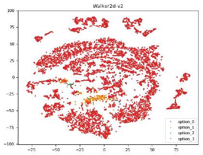
[OC] [OC+HD]

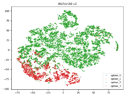
Figure 5: t-SNE plot of option-critic architecture(OC) and hd-regularization method(OC+HD) in $Walker2d$. Each point represents a state and the color of the point is an option used in the state.

The second group learns to use more than one option, such as Walker2d and Swimmer. In this case, the option-critic architecture seems to play a sufficient role. However, as shown in Fig.5, the options learned in the option-critic method in the Walker2d environment do not seem to be disentangled at all. Fig. 5 is a t-SNE analysis of the options learned from the option-critic method and the proposed method. Respectively, t-SNE analysis allows you to see how each option is spread on each axis represented by the key features. In the case of the option-critic method, the network picked 2 major options but the options shown in the t-SNE plot for the Walker2d environment were not separated. However, in our method, we could visually confirm that each option was very disentangled. This suggests that each of the options in the proposed method can be interpreted as distributing roles by learning different functions compared to the option-critic method, which is advantageous for temporal abstraction.

HD Environment OC OC+HD Hopper 0.79$\pm$0.12 0.99$\pm$0.02 HalfCheetah 0.84$\pm$0.14 1.00$\pm$0.002 Swimmer 0.59$\pm$0.12 0.99$\pm$0.02 Walker2d 0.92$\pm$0.06 1.0$\pm$0.004

Table 7: An average distance between options and its standard deviation from option-critic architecture(OC) and hd-regularization method(OC+HD) measured by HD in MuJoCo Environment.

5.2.2 Analysis with Measure

We tried to compare HD as well as various measures in MuJoCo environment. However, in the case of KLD which used in the ALE, KLD has the value of zero or infinity when the two probability distributions are entirely exclusive. For the HD, as in Table. 7, the proposed method had a value close to 1 in all environments. option-critic method had a high value in environments except Swimmer, but it did not record a higher distance than the proposed method.

5.3 Disentangling Options by Intrinsic Reward

As mentioned in Section 4.2, we can see the feasibility of using disentangled options for controlling agent by how each option is activated for intrinsic rewards. So we tested it in environments with multiple intrinsic rewards. The reward of Swimmer-v2 environment in MuJoCo implicitly consists of a control reward and a forwarding reward. The control reward is the reward for minimizing the amount of control and is inversely proportional to the absolute value of the action, and the forwarding reward is proportional to the amount of position change associated with moving the agent. In this case, as described in Table 1, the option-critic architecture uses option 1 and option 2 as major options, and our method uses option 0 and option 2 as major options. Fig. 1 is the histogram of the intrinsic rewards when each option is activated. In Fig. 1(a), the option-critic architecture, the control reward is similar in all options. And the forwarding reward has the same locality around 0 despite different variance between major options. Fig. 1(b) is the histogram of the model using the hd-regularizer. In this case, the control reward shows a similar frequency distribution to the option 0 and 2, while the forwarding reward shows different frequency distributions. In other words, the option 2 is considered to be an option optimized for maximizing the forwarding reward. From this, we can see that the options function differently in the reward aspect due to the hd-regularizer.

6 Conclusion

We have proposed an hd-regularizer that can disentangle the options. Through experiments, we compared and analyzed the learned options from the existing method and the proposed method in various perspectives. As a result, we confirmed that the proposed hd-regularizer method disentangles the intra-option policies better than the option-critic architecture from the statistical distance perspective.

Although we somehow succeeded in disentangling the options, it did not succeed in interpreting the meaning of the options represented by the non-linear approximation. In order for the options framework to have an advantage, it is important to learn the temporal abstraction representation through which it can be intuitively understood. Controlling an agent would be possible in the direction we want, based on the options supported by the interpretation. Also, the options framework, including our method, did not perform well in all RL environments. This may be due to an environment in which temporal abstraction is not essential. However, a good algorithm should be able to cope with such an environment robustly. In order to continue the study of temporal abstraction in the future, it is necessary to concentrate on the methodology that works robustly in any environment.

References

- Bacon et al. (2017) Pierre-Luc Bacon, Jean Harb, and Doina Precup. The option-critic architecture. In AAAI, pages 1726–1734, 2017.
- Bellemare et al. (2013) Marc G Bellemare, Yavar Naddaf, Joel Veness, and Michael Bowling. The arcade learning environment: An evaluation platform for general agents. Journal of Artificial Intelligence Research, 47:253–279, 2013.
- Cover and Thomas (2012) Thomas M Cover and Joy A Thomas. Elements of information theory. John Wiley & Sons, 2012.
- Csiszár (1967) Imre Csiszár. Information-type measures of difference of probability distributions and indirect observation. studia scientiarum Mathematicarum Hungarica, 2:229–318, 1967.
- Csiszár et al. (2004) Imre Csiszár, Paul C Shields, et al. Information theory and statistics: A tutorial. Foundations and Trends® in Communications and Information Theory, 1(4):417–528, 2004.
- Dayan and Hinton (1993) Peter Dayan and Geoffrey E Hinton. Feudal reinforcement learning. In Advances in neural information processing systems, pages 271–278, 1993.
- Dietterich (1998) Thomas G Dietterich. The maxq method for hierarchical reinforcement learning. In ICML, volume 98, pages 118–126. Citeseer, 1998.
- Drescher (1991) Gary L Drescher. Made-up minds: a constructivist approach to artificial intelligence. MIT press, 1991.
- Fikes et al. (1972) Richard E Fikes, Peter E Hart, and Nils J Nilsson. Learning and executing generalized robot plans. Artificial intelligence, 3:251–288, 1972.
- Harb et al. (2017) Jean Harb, Pierre-Luc Bacon, Martin Klissarov, and Doina Precup. When waiting is not an option: Learning options with a deliberation cost. arXiv preprint arXiv:1709.04571, 2017.
- Harutyunyan et al. (2017) Anna Harutyunyan, Peter Vrancx, Pierre-Luc Bacon, Doina Precup, and Ann Nowe. Learning with options that terminate off-policy. arXiv preprint arXiv:1711.03817, 2017.
- Hellinger (1909) E. Hellinger. Neue begründung der theorie quadratischer formen von unendlichvielen veränderlichen. J. Reine Angew. Math., 136:210–271, 1909.
- Iba (1989) Glenn A Iba. A heuristic approach to the discovery of macro-operators. Machine Learning, 3(4):285–317, 1989.
- Kaelbling (1993) Leslie Pack Kaelbling. Hierarchical learning in stochastic domains: Preliminary results. In Proceedings of the tenth international conference on machine learning, volume 951, pages 167–173, 1993.
- Kingma and Welling (2013) Diederik P Kingma and Max Welling. Auto-encoding variational bayes. arXiv preprint arXiv:1312.6114, 2013.
- Korf (1983) Richard E Korf. Learning to solve problems by searching for macro-operators. Technical report, CARNEGIE-MELLON UNIV PITTSBURGH PA DEPT OF COMPUTER SCIENCE, 1983.
- Kuipers (1979) Benjamin Kuipers. Commonsense knowledge of space: Learning from experience. In Proceedings of the 6th International Joint Conference on Artificial Intelligence - Volume 1, IJCAI’79, pages 499–501, 1979.
- Kullback and Leibler (1951) Solomon Kullback and Richard A Leibler. On information and sufficiency. The annals of mathematical statistics, 22(1):79–86, 1951.
- Lin (1991) Jianhua Lin. Divergence measures based on the shannon entropy. IEEE Transactions on Information theory, 37(1):145–151, 1991.
- Maaten and Hinton (2008) Laurens van der Maaten and Geoffrey Hinton. Visualizing data using t-sne. Journal of machine learning research, 9(Nov):2579–2605, 2008.
- Mann and Mannor (2014) Timothy Mann and Shie Mannor. Scaling up approximate value iteration with options: Better policies with fewer iterations. In International Conference on Machine Learning, pages 127–135, 2014.
- Mann et al. (2015) Timothy A Mann, Shie Mannor, and Doina Precup. Approximate value iteration with temporally extended actions. Journal of Artificial Intelligence Research, 53:375–438, 2015.
- Minsky (1961) Marvin Minsky. Steps toward artificial intelligence. Proceedings of the IRE, 49(1):8–30, 1961.
- Mnih et al. (2013) Volodymyr Mnih, Koray Kavukcuoglu, David Silver, Alex Graves, Ioannis Antonoglou, Daan Wierstra, and Martin Riedmiller. Playing atari with deep reinforcement learning. arXiv preprint arXiv:1312.5602, 2013.
- Parr and Russell (1998) Ronald Parr and Stuart J Russell. Reinforcement learning with hierarchies of machines. In Advances in neural information processing systems, pages 1043–1049, 1998.
- Schulman et al. (2017) John Schulman, Filip Wolski, Prafulla Dhariwal, Alec Radford, and Oleg Klimov. Proximal policy optimization algorithms. arXiv preprint arXiv:1707.06347, 2017.
- Smith et al. (2018) Matthew Smith, Herke Hoof, and Joelle Pineau. An inference-based policy gradient method for learning options. In International Conference on Machine Learning, pages 4710–4719, 2018.
- Sutton et al. (1999) Richard S Sutton, Doina Precup, and Satinder Singh. Between mdps and semi-mdps: A framework for temporal abstraction in reinforcement learning. Artificial intelligence, 112(1-2):181–211, 1999.
- Tessler et al. (2017) Chen Tessler, Shahar Givony, Tom Zahavy, Daniel J Mankowitz, and Shie Mannor. A deep hierarchical approach to lifelong learning in minecraft. In AAAI, volume 3, page 6, 2017.
- Thrun and Schwartz (1995) Sebastian Thrun and Anton Schwartz. Finding structure in reinforcement learning. In Advances in neural information processing systems, pages 385–392, 1995.
- Tieleman and Hinton (2012) T. Tieleman and G. Hinton. Lecture 6.5—RmsProp: Divide the gradient by a running average of its recent magnitude. COURSERA: Neural Networks for Machine Learning, 2012.
- Todorov et al. (2012) Emanuel Todorov, Tom Erez, and Yuval Tassa. Mujoco: A physics engine for model-based control. In Intelligent Robots and Systems (IROS), 2012 IEEE/RSJ International Conference on, pages 5026–5033. IEEE, 2012.
- Vezhnevets et al. (2016) Alexander Vezhnevets, Volodymyr Mnih, Simon Osindero, Alex Graves, Oriol Vinyals, John Agapiou, et al. Strategic attentive writer for learning macro-actions. In Advances in neural information processing systems, pages 3486–3494, 2016.
- Vezhnevets et al. (2017) Alexander Sasha Vezhnevets, Simon Osindero, Tom Schaul, Nicolas Heess, Max Jaderberg, David Silver, and Koray Kavukcuoglu. Feudal networks for hierarchical reinforcement learning. arXiv preprint arXiv:1703.01161, 2017.
- Williams and Peng (1991) Ronald J Williams and Jing Peng. Function optimization using connectionist reinforcement learning algorithms. Connection Science, 3(3):241–268, 1991.