Wetting boundaries for ternary high density ratio lattice Boltzmann method

Abstract

We extend a recently proposed ternary free energy lattice Boltzmann model with high density contrast Wöhrwag et al. (2018), by incorporating wetting boundaries at solid walls. The approaches are based on forcing and geometric schemes, with implementations optimised for ternary (and more generally higher order multicomponent) models. Advantages and disadvantages of each method are addressed by performing both static and dynamic tests, including the capillary filling dynamics of a liquid displacing the gas phase, and the self-propelled motion of a train of drops. Furthermore, we measure dynamic angles and show that the slip length critically depends on the equilibrium value of the contact angles, and whether it belongs to liquid-liquid or liquid-gas interfaces. These results validate the model capabilities of simulating complex ternary fluid dynamic problems near solid boundaries, for example drop impact solid substrates covered by a lubricant layer.

I Introduction

Understanding the flow properties of ternary fluid systems is key in many natural phenomena and technological applications. In microfluidics, combinations of immiscible liquids are employed to produce multiple emulsions Utada et al. (2005). In food sciences and pharmacology, collisions between immiscible drops Planchette et al. (2011) and liquid streams Planchette et al. (2018) can be exploited to encapsulate liquids. Collisions are also particularly relevant in combustion engines, where encapsulation of water drops by fuel can induce micro-explosions enhancing the burning rate Wang et al. (2004). Furthermore, in advanced oil recovery, the Water-Alternate-Gas (WAG) techniques are frequently employed to enhance the recovery Changlin-lin et al. (2013). The oil-water interaction in dynamic conditions also poses environmental challenges. For example the spilling of an oil layer at the surface of sea water strongly affects the production of marine aerosol when rain drops impact on the oil layer Murphy et al. (2015). In contrast, placing a lubricant layer on a rough solid is the key idea behind the recent development of Slippery Lubricant Impregnated Surfaces (SLIPS), allowing to virtually eliminate contact line pinning Smith et al. (2013); Keiser et al. (2017), with applications in coatings and packaging.

Several numerical schemes have been proposed in the recent years to simulate ternary and higher order fluid systems, including immersed boundary Hua et al. (2014), level set Merriman et al. (1994) and phase field methods Gao and Feng (2011); Kim (2012); Zhang et al. (2016); Haghani Hassan Abadi et al. (2018); Park (2018). In this work we employ the Lattice Boltzmann (LB) method Succi (2001); Krüger et al. (2017). Multiphase and multicomponent LB models are characterised by a diffuse interface, which has the advantage that the interface does not need to be tracked explicitly Kusumaatmaja et al. (2006); Kusumaatmaja and and J. M. Yeomans (2007). This makes LB models particularly convenient to study problems involving coalescence or break-up of liquids Ledesma-Aguilar et al. (2011); Komrakova et al. (2014), drop collisions Premnath and Abraham (2005); Mazloomi Moqaddam et al. (2015); Moqaddam et al. (2016); Montessori et al. (2017), drop impact on solid walls Mukherjee and Abraham (2007); Lee and Liu (2010); Banari et al. (2014); Ashoke Raman et al. (2016); Liu et al. (2015a); Andrew et al. (2017); Ashoke Raman et al. (2016) and on topographic or chemically patterned surfaces Sbragaglia et al. (2014); Mazloomi Moqaddam et al. (2017).

Several LB models have been proposed to study ternary fluid systems. Travasso et al. proposed a free energy model to study phase separation of ternary mixtures under shear Travasso et al. (2005); Spencer et al. proposed a color model to study $N>2$ component systems Spencer et al. (2010); Ridl et al. proposed a model combining N Van der Waals equation of states to study the stability of multicomponent mixtures Ridl and Wagner (2018); Semprebon et al. proposed a ternary free energy approach Semprebon et al. (2016) to model liquids with equal density, showing that the method can simulate drop morphologies on SLIPS Semprebon et al. (2017) and their dynamic properties Sadullah et al. (2018) for a wide range of surface tensions and contact angles.

To model effects of inertia, the large density ratio between liquids and the gas phase needs to be accounted Mazloomi M et al. (2015); Liang et al. (2019), but only recently ternary morels for high density ration have been proposed. Shi et al. Shi et al. (2016) extended the binary Cahn-Hilliard model for high density ratio proposed by Want et al. Wang et al. (2015) to three components. Wöhrwag et al proposed a free energy functional combining multiphase and multicomponent terms Wöhrwag et al. (2018), and employing the entropic collision approach Chikatamarla et al. (2006) could simulate density contrast up to $10^{3}$. The model could capture the salient features of head-on collisions between immiscible drops, reproducing the bouncing, adhesion and encapsulation mechanisms previously observed experimentallyPlanchette et al. (2011).

In this work we extend this high density ternary approach to model wetting of solid boundaries. The paper is organised as follows: In section II we summarise the ternary model introduced in Ref. Wöhrwag et al. (2018). In section III we perform an extensive analysis of the interfacial properties as function of the free energy parameters. In section IV we describe our implementation of three methods for wetting of solid boundaries, namely force, geometric extrapolation and geometric interpolation, and benchmark the accuracy of contact angles in mechanical equilibrium. In section V we compare the accuracy of the force and geometric interpolation methods in simulating the capillary filling of a 2D channel. In section VI we perform a ternary-specific benchmark, simulating a self-propelled bi-slug. This will enable us to evaluate the slip properties of the three fluid interfaces and assess the impact of different slip mechanisms. Finally, in section VII we summarise and discuss our results.

II Lattice Boltzmann formulation

In this section, we summarise the derivation of the multiphase-multicomponent lattice Boltzmann model proposed in Ref. Wöhrwag et al. (2018).

II.1 Ternary multiphase-multicomponent free energy

The ternary free energy model is conveniently expressed in terms of a combination of bulk $f_{\rm Bulk}$ and the interfacial terms $f_{\rm Inter}$ in the free energy functional:

$$F=\int\left[f_{Bulk}+f_{Inter}\right]dV,$$ (1)

where

$$f_{Bulk} = \frac{\lambda_{1}}{2}(\Psi_{\rm eos}(\rho)-\Psi_{0})+$$

$$\frac{\lambda_{2}}{2}C_{2}^{2}(1-C_{2})^{2}+\frac{\lambda_{3}}{2}C_{3}^{2}(1-C_{3})^{2},$$

$$f_{Inter} = \frac{\kappa_{1}}{2}(\mathbf{\nabla}\rho)^{2}+\frac{\kappa_{2}}{2}(\mathbf{\nabla}C_{2})^{2}+\frac{\kappa_{3}}{2}(\mathbf{\nabla}C_{3})^{2}.$$ (3)

The first term in Eqn. (II.1) tunes the coexistence of high density ($\rho_{l}$) liquid with a low density ($\rho_{g}$) gas. The term $\Psi_{eos}(\rho)$ is derived by integrating any suitable non ideal equation of state, $p_{eos}=\rho(d\Psi_{eos}/d\rho)-\Psi_{eos}$. In our previous work Wöhrwag et al. (2018) we have shown that the model can host various equations of state Yuan and Schaefer (2006), including van der Waals, Peng-Robinson and Carnahan-Starling. Here we employ the Carnahan-Starling equation of state:

$$\Psi_{eos}=\rho\left(C-a\rho-\frac{8RT(-6+b\rho)}{(-4+b\rho)^{2}}+RT\log(\rho)\right),$$ (4)

where the constants $C$ and $\Psi_{0}$ enforce $\Psi_{eos}(\rho_{g})=\Psi_{eos}(\rho_{l})=\Psi_{0}$. This condition ensures that the common tangent construction is valid for all coexisting phases. Unless otherwise stated, we employ the following values $a=0.037$, $b=0.2$ and $R=1$, for which the critical temperature is $T_{c}=0.3373\frac{a}{bR}$.

We define the relative concentration of the gas phase as

$$C_{1}=\frac{\rho-\rho_{l}}{\rho_{g}-\rho_{l}},$$ (5)

for which $C_{1}=0$ when $\rho=\rho_{l}$ and $C_{1}=1$ when $\rho=\rho_{g}$.

The second and third terms in Eqn. (II.1) represent a double well potential, as function of the relative liquid concentrations: $C_{2}$ and $C_{3}$. Each concentration has two minima at $C_{2,3}=0$ and $C_{2,3}=1$ corresponding to the presence or absence of the liquid. For convenience we introduce the phase field $\phi=\chi(C_{2}-C_{3})$ which, together with the density $\rho$, describes the system state. The parameter $\chi$ usually takes the value $\chi=5$ in our model, and is employed to rescale the field $\phi$ such as the distance between minima is similar in both the $\rho$ and $\phi$ fields. The variable transformations

$$C_{2}=\frac{1}{2}\left[1+\frac{\phi}{\chi}-\frac{\rho-\rho_{l}}{\rho_{g}-\rho_{l}}\right],$$ (6)

and

$$C_{3}=\frac{1}{2}\left[1-\frac{\phi}{\chi}-\frac{\rho-\rho_{l}}{\rho_{g}-\rho_{l}}\right],$$ (7)

enforce the constraint

$$C_{1}+C_{2}+C_{3}=1$$ (8)

and allow us to map the density and phase field to the concentration fields.

The bulk free energy density in Eqn. (II.1) describes three distinct energy minima in the $(\rho,\phi)$ space, corresponding to $(\rho,\phi)=(\rho_{g},0)$ (gas phase), and $(\rho_{l},+\chi)$, $(\rho_{l},-\chi)$ (liquid phases). The set of lambdas ($\lambda_{1}$, $\lambda_{2}$ and $\lambda_{3}$) tunes the magnitude of the energy barriers between each pair of phases.

Eqn. (3) contains gradient terms of the density field and the concentration of the two liquid components, describing the energy penalty in the formation of the interfaces, tuned by the set of kappas ($\kappa_{1}$, $\kappa_{2}$ and $\kappa_{3}$). Summarising, this free energy model depends on six independent parameters, to fully determine the thermodynamic properties of the system.

II.2 Derivation of the pressure tensor

The chemical potentials $\mu_{\rho}$ and $\mu_{\phi}$ are obtained directly from the free energy

$$\mu_{\rho}(\mathbf{r})=\frac{\delta F}{\delta\rho(\mathbf{r})} = \mu^{Bulk}_{\rho}+\mu^{Inter}_{\rho}$$ (9)

$$\mu_{\phi}(\mathbf{r})=\frac{\delta F}{\delta\phi(\mathbf{r})} = \mu^{Bulk}_{\phi}+\mu^{Inter}_{\phi}.$$ (10)

For convenience we express the chemical potentials in terms of the relative concentrations and, to simplify the notation, we define the auxiliary function $g(x)=x(x-1/2)(x-1)$:

$$\mu^{Bulk}_{\rho} = \frac{\lambda_{1}}{2}\frac{d\Psi_{eos}}{d\rho}-\frac{\lambda_{2}}{\Delta\rho}g(C_{2})+\frac{\lambda_{3}}{\Delta\rho}g(C_{3}),$$ (11)

$$\mu^{Bulk}_{\phi} = \frac{\lambda_{2}}{\chi}g(C_{2})-\frac{\lambda_{3}}{\chi}g(C_{3}),$$ (12)

$$\mu^{Inter}_{\rho} = -\kappa_{\rho\rho}\nabla^{2}\rho-\kappa_{\rho\phi}\nabla^{2}\phi,$$ (13)

$$\mu^{Inter}_{\phi} = \kappa_{\rho\phi}\nabla^{2}\rho-\kappa_{\phi\phi}\nabla^{2}\phi.$$ (14)

In Eqn. (11) $d\Psi_{eos}/d\rho$ is the first derivative by the density of the non ideal equation of state, and $\Delta\rho=\rho_{l}-\rho_{g}$. For the Carnahan-Starling EOS the first derivative of Eqn. (4) is

$$\frac{d\Psi_{eos}}{d\rho}=C-2a\rho+RT(1+\log\rho)+\frac{16RT(b\rho-12)}{(-4+b\rho)^{3}}.$$ (15)

Furthermore, in Eqns. (13) and (14) the mixing coefficients for the gradient terms are

$$\kappa_{\rho\rho} = \left[\kappa_{1}+\frac{\kappa_{2}+\kappa_{3}}{4(\rho_{g}-\rho_{l})^{2}}\right],$$ (16)

$$\kappa_{\phi\phi} = \frac{\kappa_{2}+\kappa_{3}}{4\chi^{2}},$$ (17)

$$\kappa_{\rho\phi} = -\frac{\kappa_{3}-\kappa_{2}}{4\chi(\rho_{g}-\rho_{l})}.$$ (18)

The pressure tensor can be inferred from the relation $\nabla\cdot\mathbf{P}=\rho\nabla\mu_{\rho}+\phi\nabla\mu_{\phi}$ and takes the form

$$P_{\alpha\beta} = p_{0}\delta_{\alpha\beta}$$

$$+ \kappa_{\rho\rho}\left[(\partial_{\alpha}\rho)(\partial_{\beta}\rho)-\left(\rho(\partial_{\gamma\gamma}\rho)+\frac{1}{2}(\partial_{\gamma}\rho)^{2}\right)\delta_{\alpha\beta}\right]$$

$$+ \kappa_{\phi\phi}\left[(\partial_{\alpha}\phi)(\partial_{\beta}\phi)-\left(\phi(\partial_{\gamma\gamma}\phi)+\frac{1}{2}(\partial_{\gamma}\phi)^{2}\right)\delta_{\alpha\beta}\right]$$

$$+ \kappa_{\rho\phi}\left[(\partial_{\alpha}\rho)(\partial_{\beta}\phi)+(\partial_{\alpha}\phi)(\partial_{\beta}\rho)\right.$$

$$\left.-\left(\rho(\partial_{\gamma\gamma}\phi)+\phi(\partial_{\gamma\gamma}\rho)+(\partial_{\gamma}\rho)(\partial_{\gamma}\phi)\right)\delta_{\alpha\beta}\right],$$

where $p_{0}$ is the pressure in the fluid bulk

$$p_{0}=\rho\mu^{Bulk}_{\rho}+\phi\mu^{Bulk}_{\phi}-f_{Bulk}.$$ (20)

II.3 Entropic Lattice Boltzmann Implementation

The dynamic evolution of the isothermic ternary system follows the continuity, Navier-Stokes, and Cahn-Hilliard equations:

$$\partial_{t}\rho+\mathbf{\nabla}\cdot\left(\rho\mathbf{v}\right)=0,$$ (21)

$$\partial_{t}(\rho\mathbf{v})+\mathbf{\nabla}\cdot\left(\rho\mathbf{v}\otimes\mathbf{v}\right)=$$

$$-\mathbf{\nabla}\cdot\mathbf{P}+\mathbf{\nabla}\cdot[\eta(\mathbf{\nabla v}+\mathbf{\nabla v^{T}})],$$ (22)

$$\partial_{t}\phi+\mathbf{\nabla}\cdot(\phi\mathbf{v})=M\nabla^{2}\mu_{\phi},$$ (23)

where $\mathbf{v}$ is the fluid velocity, $\eta$ is the dynamic viscosity, and $M$ represents the mobility in the Cahn-Hilliard model for the order parameter $\phi$.

To solve the equations of motion we introduce two sets of distribution functions, evolving the density $\rho$ and the order parameter $\phi$. For the density $\rho$, we employ the entropic lattice Boltzmann method (ELBM) Mazloomi M et al. (2015); Mazloomi M. et al. (2015),

$$f_{i}(\mathbf{x}+\mathbf{c}_{i}\Delta t,t+\Delta t)=$$

$$f_{i}(\mathbf{x},t)+\alpha\beta\left[f_{i}^{eq}(\rho,\mathbf{u})-f_{i}(\mathbf{x},t)\right]+F_{i}.$$ (24)

We implement the exact form for the equilibrium distribution function $f_{i}^{eq}(\rho,\mathbf{u})$, which for a $D$-dimensional system (described by the lattices D1Q3, D2Q9 or D3Q27) can be written in the product form Karlin et al. (1999); Ansumali et al. (2003),

$$f_{i}^{eq}=\rho w_{i}\Pi_{\alpha=1}^{D}A(u_{\alpha})[B(u_{\alpha})]^{c_{i\alpha}}.$$ (25)

The $w_{i}$’s are the lattice weights and $c_{i\alpha}$ is the $\alpha$ component of the $\mathbf{c}_{i}$-th lattice vector. The functions $A(u)$ and $B(u)$ are given by

$$A(u)=2-\sqrt{1+3u^{2}},$$ (26)

and

$$B(u)=\frac{2u+\sqrt{1+3u^{2}}}{1-u}.$$ (27)

The forcing term $F_{i}$ in Eqn. (II.3) Mazloomi Moqaddam et al. (2015) is implemented via the Exact Differences scheme

$$F_{i}=\left[f_{i}^{eq}(\rho,\mathbf{u}+\delta\mathbf{u})-f_{i}^{eq}(\rho,\mathbf{u})\right],$$ (28)

where $\rho\mathbf{u}=\sum_{i}f_{i}\mathbf{c}_{i}=\sum_{i}f^{eq}_{i}\mathbf{c}_{i}$ is the bare fluid velocity, and $\delta\mathbf{u}=(\mathbf{F}/\rho)\Delta t$ is the correction to the fluid velocity arising from the force

$$\mathbf{F}=\mathbf{\nabla}\cdot(\rho c_{s}^{2}\mathbf{I}-\mathbf{P}\bm{)}.$$ (29)

In Eqn. (29) $c_{s}^{2}=1/3$ is the speed of sound in the lattice Boltzmann scheme.

In ELBM the parameter $\beta$ tunes the kinematic viscosity $\nu=\eta/\rho=(\beta^{-1}-1)/6$, and the parameter $\alpha$ is the non-trivial root of

$$H\left(f^{\prime}+\alpha\left[f^{eq}(\rho,\mathbf{u}+\delta\mathbf{u})-f^{\prime}\right]\right)=H\left(f^{\prime}\right).$$ (30)

In Eqn. (30)

$$f^{\prime}_{i}=f_{i}+[f_{i}^{eq}(\rho,\mathbf{u}+\delta\mathbf{u})-f_{i}^{eq}(\rho,\mathbf{u})]$$ (31)

represents the mirror state, and

$$H(f)=\sum_{i}f_{i}\ln(f_{i}/w_{i}),$$ (32)

is the entropy.

To evolve the order parameter $\phi$, we employ a standard LBGK scheme

$$g_{i}(\mathbf{x}+\mathbf{c}_{i}\Delta t,t+\Delta t)=g_{i}(\mathbf{x},t)+\frac{\left[g_{i}^{eq}(\phi,\mathbf{v})-g_{i}(\mathbf{x},t)\right]}{\tau}.$$ (33)

The parameter $\tau$ is related to the mobility $M=\Gamma\left(\tau-1/2\right)$ in Eqn.(23), where the constant $\Gamma$ tunes the diffusivity and is chosen to be $\Gamma=1$ unless otherwise stated. The equilibrium distribution function, $g_{i}^{eq}(\phi,\mathbf{v})$, can be written as

$$g_{i}^{eq}(\phi,\mathbf{v}) = w_{i}\left(\frac{\Gamma\mu_{\phi}}{c_{s}^{2}}+\frac{\phi v_{\alpha}c_{i\alpha}}{c_{s}^{2}}\right.$$ (34)

$$\left.+\frac{\phi v_{\alpha}v_{\beta}\left(c_{i\alpha}c_{i\beta}-c_{s}^{2}\delta_{\alpha\beta}\right)}{2c_{s}^{4}}\right),$$

$$g_{0}^{eq}(\phi,\mathbf{v}) = \phi-\sum_{i\neq 0}g_{i}^{eq},$$ (35)

where the actual fluid velocity, $\mathbf{v}=\mathbf{u}+\delta\mathbf{u}/2$, is required.

III Surface tensions

In free energy models based on double well potentials Briant and Yeomans (2004); Briant et al. (2004), the shape of the concentration profile against the spatial coordinates takes the form of a hyperbolic tangent. This feature is inherited in our ternary model, but only for the liquid-liquid interface between phases $C_{2}$ and $C_{3}$, which is characterised by the parameter

$$\alpha_{23}=\sqrt{\frac{\kappa_{2}+\kappa_{3}}{\lambda_{2}+\lambda_{3}}}.$$ (36)

We can assume that the density does not vary at the interface between $C_{2}$ and $C_{3}$, and set $C_{1}=0$ along the interface. Following Ref. Semprebon et al. (2016), if the coordinate $x$ measures the distance from the interface along its normal direction, the concentration profiles of the components $C_{2}$ and $C_{3}$ vary according to

$$C_{2,3}(x)=\frac{1\pm\tanh{\frac{x}{2\alpha_{23}}}}{2}.$$ (37)

Integrating of the concentration profiles along $x$ we derive a simple expression for the surface tension Semprebon et al. (2016)

$$\gamma_{23}=\frac{\alpha_{23}}{6}(\lambda_{2}+\lambda_{3}).$$ (38)

For the liquid-gas interfaces, it is not possible to assume a priori that the $\rho$ and $\phi$ fields vary in the same way. Indeed, the minimization of the free energy seeks for a path which cannot be described analytically. To illustrate this aspect, we study in detail four cases, represented by the parameter sets reported in table 1. For each set we independently compute for all interfaces the surface tension $\gamma=\Delta PR$ by measuring the pressure jump $\Delta P$ across the interface of 2D drop of radius $R$ (bubble test).

set	1	2	3	4
$\bm{\lambda}_{1}$	$0.6$	$0.6$	$0.01$	$0.1$
$\bm{\kappa}_{1}$	$0.01$	$0.01$	$0.01$	$0.01$
$\bm{\lambda}_{2}$	$1.0$	$1.1$	$1.5$	$1.0$
$\bm{\kappa}_{2}$	$1.0$	$1.1$	$1.5$	$1.6$
$\bm{\lambda}_{3}$	$1.0$	$0.5$	$1.5$	$0.2$
$\bm{\kappa}_{3}$	$1.0$	$0.5$	$1.5$	$-0.4$
$\bm{\gamma}_{12}$	$0.414$	$0.431$	$0.333$	$0.321$
$\bm{\gamma}_{13}$	$0.414$	$0.334$	$0.333$	$0.120$
$\bm{\gamma}_{23}$	$0.323$	$0.259$	$0.485$	$0.180$
$\bm{\theta}_{1}$	$134.1$	$143.1$	$86.3$	$-$
$\bm{\theta}_{2}$	$112.9$	$129.2$	$136.8$	$-$
$\bm{\theta}_{3}$	$112.9$	$87.6$	$136.8$	$-$

Table 1: Parameters of four selected sets, and the relative surface tensions and Neumann angles. The last row reports the global energy minimum configuration of a double emulsion. The white region corresponds to the gas phase ($C_{1}$), while the blue and red regions correspond to the liquids $C_{2}$ and $C_{3}$.

The 4 sets are listed in order of increasing mismatch between the interfacial profiles. The first set represents two liquids with symmetric properties, where the liquid-liquid surface tension is slightly lower than both the liquid-gas ones. The second set describes three fluids with different properties. The third set also describes two equal liquids but $\lambda_{1}$ is much smaller than in the first set, leading to a liquid-liquid surface tension significantly larger than the liquid-gas ones. The fourth set describes also three fluids, but in this case the parameter $\kappa_{3}$ is negative, leading to a spontaneous encapsulation of liquid $C_{2}$ by liquid $C_{3}$. Negative values of lambdas or kappas are generally allowed in the ternary model, as long as the three minima in the $[\rho,\phi]$ space are well defined.

In Fig. 2 we inspect the properties of the diffuse interfaces for the parameter sets described in table 1. The color maps illustrate the contours of the bulk free energy in the $[\phi,\rho]$ space. As expected, the bulk free energy is symmetric in $\phi$ for sets 1 and 3, and non-symmetric for sets 2 and 4.

Introducing the variable transformation Eqns. 5, 6 and 7 into Eqn. 8 we can easily see that the absence of the third component at any interface leads to a linear relation between $\rho$ and $\phi$ connecting the corresponding minima, represented by straight lines in the $[\rho,\phi]$ space in Fig. 2. However, the minimisation of the free energy does lead to different paths, depicted by connected dots. As Eqn. 8 must be satisfied, the inverse variable transformation will produce a certain fraction of the minor component at the interface.

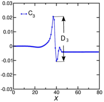
Figure 1: (Color online) Example of profile of the concentration $C_{3}$ at the interface between $C_{1}$ and $C_{2}$ illustrating the definition of the Deformation Coefficient ($D_{3}$).

For set 1 the interface path is close to the “ideal” profile. The deviations in the remaining sets increase with the increasing mismatch between the profiles of $\rho$ and $\phi$. To quantify these mismatches we define the “Deformation coefficient” $D$ as the difference between the maximum and minimum values of the minority phase in a region $\Omega$ near the interface between the two majority phases. For example, at the interface between $C_{1}$ and $C_{2}$, the Deformation coefficient $D_{3}$ is defined as

$$D_{3}=\max_{\mathbf{x}\in\Omega}(C_{3})-\min_{\mathbf{x}\in\Omega}(C_{3}),$$ (39)

and similarly for the other interfaces.

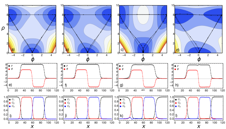
Figure 2: (Color online) Upper row: color maps of the bulk free energy for the parameter sets 1,2,3 and 4 (panels a,b,c and d). The dashed lines connecting the three energy minima represent the path in the of $[\phi,\rho]$ space of an ideal interface, where the third components is completely absent. Data points represent the path of the numerically computed interface profiles in mechanical equilibrium. Deviations from the dashed lines reveal the creation of a fraction of concentration the third component. Middle row (panels e,f,g and h): Profiles of $\rho$ and $\phi$ along interfaces between fluids, placed in the sequence $1,2,3,1$. Bottom row (panels i,j,k and l): Profiles of $C_{1}$, $C_{2}$ and $C_{3}$ along interfaces between fluids in the corresponding sequence $1,2,3,1$.

subspace	$\bm{\lambda}_{1}$	$\bm{\lambda}_{2}$	$\bm{\lambda}_{3}$	$\bm{\kappa}_{1}$	$\bm{\kappa}_{2}$	$\bm{\kappa}_{3}$
1	$Y$	$X$	$X$	$0.01$	$X$	$X$
2	$Y$	$X$	$X$	$0.01$	$0.5X$	$0.5X$
3	$Y$	$X$	$0.5$	$0.01$	$X$	$0.5$
4	$0.01$	$X$	$Y$	$0.01$	$X$	$Y$
5	$0.5$	$X$	$Y$	$0.01$	$X$	$Y$
6	$1.0$	$X$	$Y$	$0.01$	$X$	$Y$
7	$Y$	$X$	$0.5$	$0.01$	$2X-0.5$	$1-X$
8	$0.1$	$X$	$1.0$	$0.01$	$Y$	$1+X-Y$

Table 2: Summary of surface tension tests. Details for each case in supplementary information.

To quantify the interfacial properties arising in the ternary model, we have carried out a systematic analysis for a wide range of parameters. Because a complete scan of the six-dimensional parameter space formed by ${\bm{\lambda}}=(\lambda_{1},\lambda_{2},\lambda_{3})$ and ${\bm{\kappa}}=(\kappa_{1},\kappa_{2},\kappa_{3})$ is too demanding, we have identified eight subspaces. Each subspace is a two-dimensional map defined by the coordinates, $X$ and $Y$. Subspaces are divided in a $20\times 20=400$ points grid, and for each point, representing a specific parameter set, we perform three independent measures of the surface tensions (one for each interface). Each surface tension is obtained from a bubble test, introducing a drop of radius $80$ lattice units, within a simulation domain of $320\times 320$ lattice units. In all tests we set $T_{red}=0.61$, leading to an effective density ratio $\rho_{l}/\rho_{g}\simeq 10^{3}$.

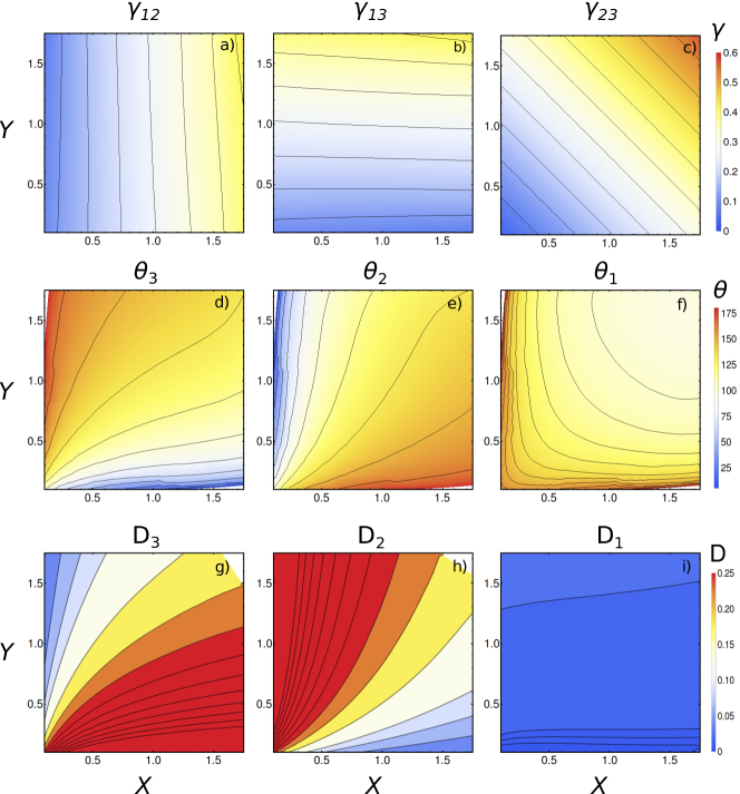
Figure 3: (Color online) Colour maps of relevant quantities as function of the coordinate $X=\lambda_{2}$ and $X=\lambda_{3}$ Upper row (a,b,c): surface tensions ($\lambda_{12}$, $\lambda_{13}$ and $\lambda_{23}$); Middle row (d,e,f): Neumann angles ($\theta_{3}$, $\theta_{2}$ and $\theta_{1}$); Lower row (g,h,i): Deformation coefficient ($D_{3}$, $D_{2}$ and $D_{1}$).

The maps ${\bm{\lambda}}(X,Y)$ and ${\bm{\kappa}}(X,Y)$ are summarised in table 2. In subspace 1 we consider liquids with identical properties $\lambda_{2}=\lambda_{3}=\kappa_{2}=\kappa_{3}=X$ and explore the relative impact of the liquid-gas component $\lambda_{1}=Y$. Subspace 2 is similar, but the liquid-liquid width is larger and the range of $\lambda_{1}=Y$ is extended to negative values, providing combinations of parameters for liquids repelling each other. In subspace 3 we fix $\lambda_{3}=\kappa_{3}=0.5$, and explore the interplay between the gas phase and the first liquid. In subspace 4, 5 and 6 we fix the the weight of the bulk term for the equation of state to three values $\lambda_{1}=0.01,0.6,1.0$, representing respectively small, medium and large contribution to the liquid-gas component of the surface tension, and systematically explore the combinations of the two liquids. In subspaces 7 and 8 we explore combinations with negative values of $\kappa_{2}$, allowing us to achieve encapsulation of liquid 3 by liquid 2.

In Fig. 3 we report, as an example, our analysis of the subspace 4. The first row of panels depicts the surface tensions $\gamma_{12}$, $\gamma_{13}$ and $\gamma_{23}$ respectively. As expected, $\gamma_{12}$ and $\gamma_{13}$ mainly depend on the variation of $X=\lambda_{2}$ and $Y=\lambda_{3}$ respectively, while $\gamma_{23}$ is function of $X+Y=\lambda_{2}+\lambda_{3}$. The non perfect alignment of the contour lines with the main axes for $\gamma_{12}$ and $\gamma_{13}$ is an indication of the non constant contribution of the liquid-gas component, even if $\lambda_{1}$ is fixed throughout the subspace. The variation of $\gamma_{23}$ instead is more regular, because no variation of the density field occurs at this interface, and closely follows the values of surface tension predicted by Eqn. (38) (comparison not shown).

The second row of panels in Fig. 3 reports the Neumann angles $\theta_{1}$, $\theta_{2}$ and $\theta_{3}$ computed as functions of the surface tensions:

$$\cos\theta_{1}=\frac{\gamma_{23}^{2}-\gamma_{12}^{2}-\gamma_{13}^{2}}{2\gamma_{12}\gamma_{13}},$$ (40)

$$\cos\theta_{2}=\frac{\gamma_{13}^{2}-\gamma_{12}^{2}-\gamma_{23}^{2}}{2\gamma_{12}\gamma_{23}},$$ (41)

$$\cos\theta_{3}=\frac{\gamma_{12}^{2}-\gamma_{13}^{2}-\gamma_{23}^{2}}{2\gamma_{13}\gamma_{23}}.$$ (42)

For the full range of parameters explored in this subspace, the Neumann angles are always well defined, indicating that the spreading parameter $S_{k}=\gamma_{ij}-\gamma_{ik}-\gamma_{jk}<0$. The third row of panels in Fig. 3 reports the “Deformation coefficient” $D$, measured for each interface. As expected, $D_{1}\simeq 0$ throughout the whole map. In contrast, $D_{2}$ and $D_{3}$ vary up to $25\%$ of the concentration interval ($[0,1]$).

For each subspace in table 2 we have fitted the maps of surface tension with a two-variable polynomial function. We report in the supplementary material a detailed description, including fitting functions for the surface tensions, of each subspace. This database can provide guidance to select the free energy parameters and reproduce target combinations of surface tensions.

IV Solid Boundaries

In this section we describe and benchmark our implementation of solid boundaries. For simplicity we consider only flat walls, aligned with the domain axis and located at half distance between lattice nodes, but all methods can be easily extended to solid structures with corners and wedges.

In all methods we treat the first layer of solid nodes as ghost nodes, to store values of $\rho$ and $\phi$. These values are employed in the finite difference stencils to compute $\nabla\rho$, $\nabla\phi$, $\nabla^{2}\rho$ $\nabla^{2}\phi$, in order to evaluate the chemical potentials and the pressure tensor (Eqns. (13), (14), (II.2)) of the fluid near the solid boundaries, as illustrated in Fig. 4 (a)

Throughout the whole fluid domain, the forces are computed by numerically differentiating the pressure tensor in Eqn. (29). As $\mathbf{P}$ is not defined on the solid nodes, its partial derivatives in the first fluid layer are computed differently. Specifically, near the solid boundaries we impose $\mathbf{\nabla}\mathbf{P}_{\perp}=0$ (perpendicular to the solid), while a one-sided biased gradient Lee and Liu (2010) is employed for the gradient $\mathbf{\nabla}\mathbf{P}_{\parallel}$ (parallel to the solid), as illustrated in Fig. 4 (a). After the collision and streaming steps, standard bounce-back rules are applied Ladd (1994).

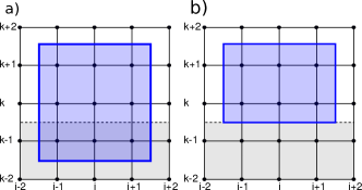
Figure 4: (Color online) Sketch in 2D of the stencils employed for the computation of gradients. (a) The stencil for $\nabla\rho$, $\nabla\phi$, $\nabla^{2}\rho$ and $\nabla^{2}\phi$ is the same as in the fluid bulk, and relies on the quantities stored in the ghost nodes in the solid layer. (b) The stencil for $\mathbf{\nabla}\mathbf{P}_{\parallel}$ excludes solid nodes, where $\mathbf{P}$ is not defined.

IV.1 Method 1 (force)

The forcing method Huang et al. (2007); Mazloomi M. et al. (2015) is inspired by pseudo-potential models for multicomponent fluids, where the liquid-solid interaction is introduced through a forcing term. In our implementation, the values of $\rho$ and $\phi$ in the ghost nodes at the solid layer are constantly updated by copying the values in the first fluid layer. This procedure alone gives to the solid neutral wetting properties. In this method, higher or lower affinity of the fluid phases to the solid are obtained by adding a local force term:

$$\mathbf{F}_{s}(\mathbf{x},t)=\rho^{rel}(\mathbf{x})\left(\kappa_{\rho}^{w}+\phi^{rel}(\mathbf{x})\kappa_{\phi}^{w}\right)\sum_{i}w_{i}s(\mathbf{x}+\mathbf{c}_{i}\delta t)\mathbf{c}_{i}.$$ (43)

where $s$ is a function that takes a value of $1$ on fluid nodes connected two lattice vectors away from solid nodes. In practice, for a flat substrate as in the sketch in Fig. 5, $s$ takes value 1 on the second layer of fluid nodes only. We apply the force to the second fluid layer instead of the first one (as proposed in other works Mazloomi M. et al. (2015)), to improve the stability of the algorithm. One can easily verify that force terms of smaller magnitude are necessary at the second fluid layer to obtain the same target contact angle.

The pre-factor $\rho^{rel}(\mathbf{x})\left(\kappa_{\rho}^{w}+\phi^{rel}(\mathbf{x})\kappa_{\phi}^{w}\right)$ accounts for the variation of the interaction strength as function of the fields $\rho$ and $\phi$, tuned by the parameters $\kappa_{\rho}^{w}$ and $\kappa_{\phi}^{w}$. We employ the rescaled fields $\rho^{rel}(\mathbf{x})=(\rho(\mathbf{x})-\rho_{g})/(\rho_{l}-\rho_{g})$ and $\phi^{rel}(\mathbf{x})=\phi(\mathbf{x})/\chi$, which vary in the interval $[0,1]$ and $[-1.1]$ respectively.

Furthermore, for the stability of the algorithm it is essential that no large forcing terms are applied in the gas phase ($[\rho,\phi]=[\rho_{g},0]$), which is achieved by multiplying both $\kappa_{\rho}^{w}$ and $\kappa_{\phi}^{w}$ by $\rho^{rel}(\mathbf{x})$ in our approach. In absence of this precaution, large forcing terms would cause strong deviations of the gas density from the equilibrium thermodynamic value.

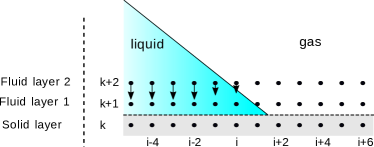
Figure 5: (Color online) Sketch of the forcing terms acting near the liquid-liquid interface in contact to a solid boundary. The arrows represent the direction and magnitude of the local force Eqn. (43).

When defining a contact angle between two phases we indicate with the first index the phase in which a contact angle is measured, and with the second index the other phase. In our work we adopt the convention of measuring the angles in the liquid phase at liquid-gas interfaces, while at the liquid-liquid interface we measure the angle in the liquid with index 2. The following relations are implied: $\theta_{12}=\pi-\theta_{21}$, $\theta_{13}=\pi-\theta_{31}$ and $\theta_{32}=\pi-\theta_{23}$.

A typical dependence of $\theta_{21}$, $\theta_{31}$ and $\theta_{23}$ from the parameters $\kappa_{\rho}^{w}$ and $\kappa_{\phi}^{w}$ is reported in Fig. 6 (panels a-c), for the parameter set 1 in table 1. Contact angles are measured after equilibrating 2D sessile drops for each interface and fitting the drop interfaces with circular profiles. To keep the accuracy of the contact angle, across the whole parameter range, the drop area is fixed to $\simeq 100^{2}$l.u.² while the size and aspect ratio of the simulation domain is adjusted to accommodate drops of different shapes.

The maps, as shown in Fig. 6, are specific for each set of free energy parameters. For example the inclination of the diagonal contour lines of $\theta_{21}$, $\theta_{31}$ depends on the value of the surface tension for each interface. $\theta_{23}$ instead is predominantly a function of $\kappa_{\phi}^{w}$, with only a residual dependence on $\kappa_{\rho}^{w}$ in the region of small $\kappa_{\phi}^{w}$.

On ideal surfaces the combinations of contact angles are not independent, but obey the Girifalco-Good relation Girifalco and Good (1957), which according to our convention reads

$$0=\Delta\gamma=\gamma_{23}\cos\theta_{23}-\gamma_{13}\cos\theta_{31}+\gamma_{12}\cos\theta_{21}$$ (44)

This condition is automatically satisfied by the force method, as can be deduced from panel d) in Fig. 6, which reports the variation of $\Delta\gamma$ on a scale set by the largest value surface tension in the system ($\gamma_{\rm max}\simeq 0.5$). Small deviations identified by the contour lines can be attributed to the uncertainties in the measurement of the contact angles.

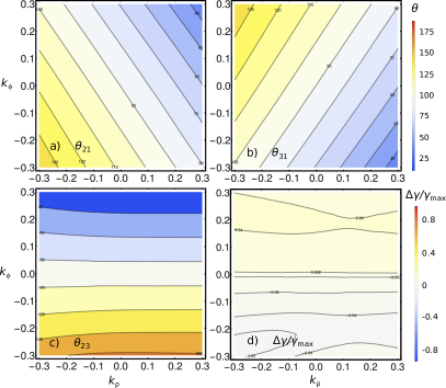
Figure 6: (Color online) Colour maps of equilibrium contact angles measured from sessile drops, as function of $\kappa_{\rho}^{w}$ and $\kappa_{\phi}^{w}$. Panels a-c) refer to the interfaces $[1,2]$, $[1,3]$ and $[2,3]$ respectively. Panel d) reports the quantity $\Delta\gamma$, (Eqn. 44). The combinations of surface tensions are given by the first set in table 1.

IV.2 Method 2 and 3 (geometric approaches)

We now introduce the two geometric approaches employed in our model. The key idea in both models is to manipulate the values of the fields in the ghost nodes at the solid boundaries according to a geometrical criterion, in order to reproduce a prescribed contact angle. In both cases, the ternary implementation requires us to identify in advance the correct interface, in order to select the correct target contact angle. This step is performed by implementing a set of rules that combine the local value of $\rho$ and $\phi$ and of their gradients parallel to the solid $\nabla_{\parallel}\rho$ and $\nabla_{\parallel}\phi$:

$$\begin{cases}\text{if }|\nabla_{\parallel}\rho|/|\nabla_{\parallel}\phi|<0.01(\rho_{l}-\rho_{g})/\chi&\text{set interface 2-3}\\ \text{if }\nabla_{\parallel}\rho\cdot\nabla_{\parallel}\phi<0&\text{set interface 1-3}\\ \text{if }\nabla_{\parallel}\rho\cdot\nabla_{\parallel}\phi>0&\text{set interface 1-2}\\ \text{if }\rho>\rho_{l}/2\text{ and }\phi<-0.95\chi&\text{set interface 1-3}\\ \text{if }\rho>\rho_{l}/2\text{ and }\phi>0.95\chi&\text{set interface 1-2}\\ \end{cases}$$

This set of rules proves to be accurate in all our tests, even if the variation of $\rho$ and $\phi$ is not strictly monotonous near the interface. An alternative approach consists in weighting the contact angles based on the local concentration fields Zhang et al. (2016).

Geometric extrapolation - We now introduce our ternary implementation of the method proposed by Ding and Spelt Ding and Spelt (2007). The key idea is to compute the normal vector of a fluid interface in contact with the solid surface from the gradient of a field: $\mathbf{n}_{s}=\nabla c/|\nabla c|$. We employ $c=\rho$ at any liquid-gas interface, and $c=\phi$ for the liquid-liquid interface. Referring to the sketch of the contact line geometry in Fig. 7, $\mathbf{n}$ defines the vector normal to a plane solid surface, while the perpendicular and parallel components of a field gradient can be expressed as $\nabla c_{\perp}=\mathbf{n}\cdot\nabla c$ and $\nabla c_{\parallel}=|\nabla c-(\mathbf{n}\cdot\nabla c)\mathbf{n}|$.

In the algorithm, first the parallel component of the gradient $\nabla c_{\parallel}$ is measured along the surface, and then it is employed to reconstruct the perpendicular component of the gradient $\nabla c_{\perp}$. For a diffuse interface forming an angle $\theta$ with the solid surface, the relation between components of the field gradients is

$$\nabla c_{\perp}=\tan\left(\frac{\pi}{2}-\theta\right)\nabla c_{\parallel}.$$ (45)

For example, in a 2D lattice addressed by the indices $i,k$, let us assume the layer $k$ represents a solid surface for any $i$, while the layer $k+1$ represents the first fluid layer. The values of the field $c_{i,k}$ are computed by extrapolating the from the field value in the above layer

$$c_{i,k}=c_{i,k+1}+\nabla c_{\perp},$$ (46)

where $c$ represents either $\rho$ or $\phi$. For this reason, we denote this method as geometric extrapolation.

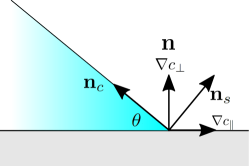
Figure 7: (Color online) Sketch of the main vectors defined by fluid interface near the contact line.

The 3D implementation differs from the 2D case only by replacing the component parallel to the surface of the concentration gradients with the norm of the two components in the plane. For example, if $x$ and $y$ define the coordinates in the plane, we have $|\nabla_{\parallel}c|=\sqrt{(\nabla_{x}c)^{2}+(\nabla_{y}c)^{2}}$ for a solid plane at $z={\rm const}$. The correction applies both in the determination of the interface, and in the reconstruction of the perpendicular component $\nabla_{\perp}c$.

In contrast to the force approach, there is no limitation in choosing any combination of contact angles, keeping in mind that a physically consistent set of contact angles needs to fulfil the Girifalco-Good relation in Eqn. (44). We will take advantage of combinations of angles not fulfilling Eqn. (44) to simulate self propelled bi-slugs in a channel in Sec. VI.

Geometric interpolation - This third method is inspired by the algorithm proposed by Lee and Kim Lee and Kim (2011). Here the key idea is to interpolate the field values from the upper layer, where the interpolating point is shifted according to the slope of the liquid interface.

For a few special values of contact angles the slope of the interface connects to lattice nodes, and the required values of the field correspond exactly to the values already stored. Let us consider a 2D example: for the three nearest lattice nodes along the direction $i$ of the solid surface we can simply assign

$$c_{i,k}|_{\theta\simeq 18.43^{\circ}} =c_{i-3,k+1}$$

$$c_{i,k}|_{\theta\simeq 26.56^{\circ}} =c_{i-2,k+1}$$

$$c_{i,k}|_{\theta=45^{\circ}} =c_{i-1,k+1}$$

$$c_{i,k}|_{\theta=90^{\circ}} =c_{i,k+1}$$

$$c_{i,k}|_{\theta=45^{\circ}} =c_{i+1,k+1}$$

$$c_{i,k}|_{\theta\simeq 153.43^{\circ}} =c_{i+2,k+1}$$

$$c_{i,k}|_{\theta\simeq 161.56^{\circ}} =c_{i+3,k+1}.$$

For any other slope instead we linearly interpolate the values of the two closest nodes. For this reason we denote this method as geometric interpolation. As shown in Fig. 8 (a), in the 2D implementation we compute the distance of the interpolating point from the node $i$ as $l_{\parallel}=\tan(\theta-\pi/2)$. In a local coordinate system centred in the node $(i,k)$, the interpolating points are located at $l_{0}={\rm floor}(l_{\parallel})$ and $l_{1}={\rm floor}(l_{\parallel})+1$, and their lattice indices are $i_{0}=i+l_{0}$ and $i_{1}=i+l_{1}$. Considering that $l_{1}-l_{0}=1$, the linear interpolation scheme is

$$c_{i,k}=(c_{i_{1},k+1}-c_{i_{0},k+1})l_{\parallel}+(l_{1}c_{i_{0},k+1}-l_{0}c_{i_{1},k+1}).$$ (48)

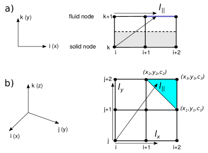
Figure 8: (Color online) Sketch of the geometry interpolation boundaries: a)2D implementation: the selected interval for the linear interpolation is highlighted. b)3D implementation: the selected triangle for the planar interpolation is highlighted.

The 3D implementation requires the selection of an appropriate support for the interpolation in the plane. As in the previous case, let us assume a solid surface defined by the plane plane $z={\rm const}$, where solid nodes have constant index $k$ and the first fluid layer is at $k+1$. Also, the lattice nodes in the planes parallel to the solid surface are addressed by the indices $i$ and $j$. The location of the interpolating points is determined by the gradients of the concentration field in the plane $l_{x}=l_{\parallel}\nabla_{x}c/|\nabla c_{\parallel}|$ and $l_{y}=l_{\parallel}\nabla_{y}c/|\nabla c_{\parallel}|$. The simplest interpolation scheme for a plane in 3D requires three points. In our implementation we select the three furthest points (out of four) from the location $(i,j)$ in a planar square lattice (cfr. the sketch in Fig. 8 (b).

Once the three points are selected, we consider the three triplets $(x_{1},y_{1},c_{1})$, $(x_{2},y_{2},c_{2})$ and $(x_{3},y_{3},c_{3})$, describing a plane, where the third coordinate represents the value of the concentration $c$ in each point. The following interpolation scheme is employed to compute the field values in the ghost node located in $(i,j,k)$:

$$c_{i,j,k}=\frac{Al_{x}+Bl_{y}+C}{D},$$ (49)

where $A,B,C,D$ are the polynomials

$$A= y_{2}c_{1}-y_{3}c_{1}-y_{1}c_{2}+y_{3}c_{2}+y_{1}c_{3}-y_{2}c_{3}$$

$$B= -x_{2}c_{1}+x_{3}c_{1}+x_{1}c_{2}-x_{3}c_{2}-x_{1}c_{3}+x_{2}c_{3}$$

$$C= -x_{3}y_{2}c_{1}+x_{2}y_{3}c_{1}+x_{3}y_{1}c_{2}$$

$$-x_{1}y_{3}c_{2}-x_{2}y_{1}c_{3}+x_{1}y_{2}c_{3}$$

$$D= -x_{2}y_{1}+x_{3}y_{1}+x_{1}y_{2}-x_{3}y_{2}-x_{1}y_{3}+x_{2}y_{3}.$$ (50)

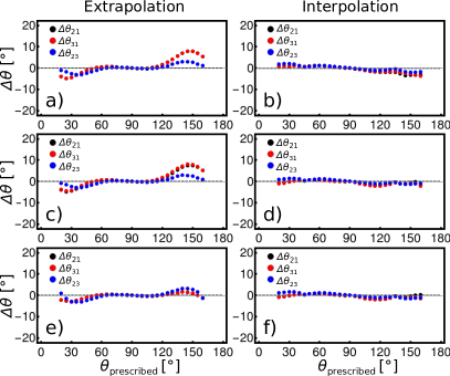
Figure 9: (Color online) Deviation of contact angles $\theta_{21}$, $\theta_{31}$ and $\theta_{23}$, measured on sessile drops in mechanical equilibrium from the prescribed values. Results for the geometric extrapolation method (left column) and the geometric interpolation method (right column). The interfacial properties correspond to set 1 (first row); set 2 (second row); and set 3 (first row) listed in table 1.

We have assessed the accuracy of both geometric methods by simulating sessile drops in mechanical equilibrium for each fluid-fluid interface and comparing the parameter sets 1, 2 and 3 in table 1. The simulation setup and analysis are the same as previously employed to validate the force method. In the intermediate range of angles $[60^{\circ},120^{\circ}]$ both methods show good agreement, with deviations below $1^{\circ}$, while for larger and smaller angles the geometry interpolation method is to be preferred. In view of this result, we discard the extrapolation in favour of the interpolation method for the remaining tests.

V Capillary filling

To assess the dynamic properties of fluid interfaces, we simulate the capillary filling of a channel by a liquid. The problem was studied independently by Richard Lucas Lucas (1918) and Edward Washburn Washburn (1921). It represents a classical benchmark for wetting boundary conditions in lattice Boltzmann implementations Wiklund et al. (2011); Liu et al. (2015b); Lou et al. (2018), as it provides analytical or semi-analytical expressions to compare.

Let us now consider the system sketched in Fig. 10 , consisting in a 2D channel of height $H$, initially containing a gas phase only, and filled by liquid. The liquid-gas surface tension is denoted by $\gamma$, while the liquid forms a contact angle $\theta$ with the solid.

In a 2D geometry, the driving capillary force is applied at the two contact points of the liquid interface with the channel walls:

$$F^{\rm cap}=2\gamma\cos\theta.$$ (51)

Except for the initial transient time, the resisting force is mainly provided by viscous dissipation. In virtue of the high density ratio in our model, we neglect the dissipation in the gas phase Diotallevi et al. (2009). For a liquid of viscosity $\mu=\rho_{l}\nu$ forming a column of length $x$, and assuming a fully developed Poiseuille velocity profile, we have a resisting force

$$F^{\rm visc}=-\frac{12\rho_{l}\nu x\dot{x}}{H},$$ (52)

where $\dot{x}$ is the mean velocity of the fluid column, corresponding to the velocity of the liquid-gas interface. Eqns. (51) and (52) lead to the so-called Washburn law

$$x(t)=K\sqrt{(t-t_{0})},$$ (53)

where $t_{0}$ is a time constant. The pre-factor

$$K=\sqrt{\frac{\gamma\cos\theta H}{3\nu\rho_{l}}},$$ (54)

is function of material and geometric parameters only: the surface tension $\gamma$, the equilibrium contact angle $\theta$, the kinematic viscosity $\nu$ of the liquid and channel height $H$.

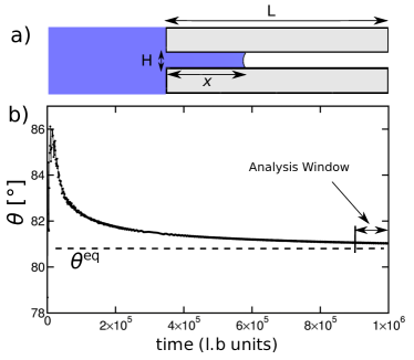
Figure 10: (Color online) Capillary filling: (a) Sketch of the simulation setup; (b) Dynamic contact angle vs simulation time for the Geometric Interpolation method and $\theta_{21}=80^{\circ}$. The analysis window consists of the last $10\%$ of the simulation time, over which the dynamic contact angle is averaged.

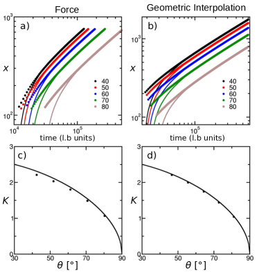
Figure 11: (Color online) Capillary filling: (a,b) Length of the liquid column vs simulation time for contact angles $\theta=40^{\circ},50^{\circ},60^{\circ},70^{\circ}$ and $80^{\circ}$. Dots represent numerical results, while continuous lines data fits. (c,d) Pre-factor $K$ for the Lucas-Washburn law. Dots represent fits to the numerical results, the continuous line is the model prediction (Eqn. (54)). Left panels (b,d) are obtained employing the force method, while right panels (c,e) employ the geometric interpolation method.

In our simulations the channel length is $L=2000$ l.u. and the height $H=70$l.u. The channel is preceded and followed by reservoirs filled with liquid and gas respectively. This geometry has been previously employed Diotallevi et al. (2009) to minimise the viscous drag of the fluid outside the channel. Throughout all simulations we employ the first parameter set in table 1, for which $\gamma=0.414$ in both liquid-gas interfaces, and set $\beta=0.5$, giving a kinematic viscosity $\nu=1/6=0.16667$.

In Fig. 11 (a,b) we report the time evolution of the front of the liquid column for contact angles varied in the range of $[30^{\circ},80^{\circ}]$, comparing the force and geometric interpolation methods. The initial stage of the invasion is not well described by Wahsburn law Diotallevi et al. (2009). As shown in Fig. 10 (b), during the filling process the dynamic angle varies over time, and approaches the equilibrium value only asymptotically. Consequently, Washburn law, Eqn. 53 describes accurately only the asymptotic regime, while for the initial and transient regimes inertia and viscous bending should also be considered.

As in this specific test our main interest is comparing the accuracy of the force and geometric interpolation methods, we analyse the last $10\%$ of the simulation time, where the variation of dynamic angles are below one degree, and we can assume Eqn. 53 to be sufficiently accurate. To eliminate systematic sources of errors, we compute the average dynamic angle $<\theta>$ within the analysis window, and replace with it the angle $\theta$ in Eqn. (54). Furthermore, we perform a parametric fit of the numerical data within the analysis window with Eqn. (53), and compute the time constant $t_{0}$ and the pre-factor $K$.

In Fig. 11 (c,d) we compare the values of $K$ to the model (Eqn. (54)). The data for the force method show small deviations between predicted and measured values of the prefactor. The deviations increase proportionally with the magnitude of the forcing term, which increases as $\theta$ decreases. This suggests that the discrepancy is related to spurious velocities near the walls, due the force term in the force method. In contrast, we observe no deviations for the geometric interpolation.

VI Self-propelled slugs

In this section we focus on a ternary-specific benchmark, consisting in a self-propelled train of drops (bi-slug) in a 2D channel.

In experiments, a bi-slug with three finite contact angles can not self-propel, unless the Girifalco-Good relation, Eqn. (44), is broken. This may be done by introducing a step or gradient of wettability on the channel surfacesEsmaili et al. (2012); Huang et al. (2014). Alternatively, at least one liquid phase must be completely wetting. This last condition was exploited by Bico and Queré to study experimentally in detail self propelled bi-slugs Bico and Quéré (2000, 2002). Taking advantage of the geometric interpolation method, we can numerically introduce arbitrary contact angles in the system providing a controlled mechanism for self-propulsion.

The simulation geometry, sketched in Fig. 12 (a), consists of a periodic channel of height $H=39$ l.u. It contains a train of drops having equal volumes. For simplicity, we assume the length $L_{1}=L_{2}$ of each liquid drop, approximated by the length of the equivalent rectangle having the same area and height $H$. The total length of the periodic channel is adjusted in each simulations to allow the presence of at least $200$ lattice units of gas at the two sides of the bi-slug.

VI.1 Bi-slug dynamics

In long trains of drops the driving force is almost completely dissipated in the liquid bulk. Consequently the velocity is small and the contact angles remain close to the equilibrium value. According to the convention for contact angles employed in this work, the surface tension unbalance is expressed by

$$\Delta\gamma=\gamma_{23}\cos\theta_{23}-\gamma_{13}\cos\theta_{31}+\gamma_{12}\cos\theta_{21},$$ (55)

and the driving force is

$$F^{\rm cap}=2\Delta\gamma,$$ (56)

Assuming a Poiseuille flow profile in the bi-slug, and liquids with equal viscosity, the viscous force is

$$F^{\rm visc}=-\frac{12\rho_{l}\nu L\dot{x}}{H},$$ (57)

where $\dot{x}$ is the mean fluid velocity, associated to the velocity of the center of mass of the bi-slug.

In the limit of long trains ($L=L_{1}+L_{2}>>H$) the viscous bending can be neglected, and the equation of motion for the center of mass is Diotallevi et al. (2009); Esmaili et al. (2012)

$$\rho_{l}LH\ddot{x}=F^{\rm cap}+F^{\rm visc}.$$ (58)

By introducing Eqns. (56) and (57) into Eqn. (58), we obtain

$$\ddot{x}+\frac{12\nu}{H^{2}}\dot{x}-\frac{2\Delta\gamma}{\rho_{l}LH}=0.$$ (59)

Integrating once with time and imposing $\dot{x}(0)=0$, we obtain an exponential relaxation of the bi-slug velocity to the steady velocity $v_{\infty}$

$$\dot{x}(t)=v_{\infty}(1-e^{\frac{-t}{\tau_{\rm rel}}}),$$ (60)

where the steady velocity is

$$v_{\infty}=\frac{H\Delta\gamma}{6\rho_{l}\nu L}$$ (61)

and the relaxation time is

$$\tau_{\rm rel}=\frac{H^{2}}{12\nu}.$$ (62)

Integrating Eqn. (60) once again with time we obtain the displacement of the center of mass with respect to its initial position $x(0)$

$$x(t)=x(0)+\tau_{\rm rel}v_{\infty}(e^{\frac{-t}{\tau_{\rm rel}}}+\frac{t}{\tau_{\rm rel}}-1).$$ (63)

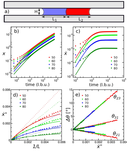
Figure 12: (Color online) Self- propeled bi-slugs: (a) Sketch of the simulation setup. The other panels report data for bi-slugs defined by the first parameter set in table 1. We set $\beta=0.5$ and contact angles $\theta_{23}$=$\theta_{21}$=$\theta_{31}=50^{\circ},60^{\circ},70^{\circ},80^{\circ}$. (b,c) Transient regime in the motion of the bi-slugs of length $L=1500$l.u., showing (b) the position and (c) the velocity of the center of mass. (d) The measured steady velocity $\dot{x}_{\infty}$ as function of $1/L$. (e) The dynamic contact angles for the three interfaces as function of $\dot{x}_{\infty}$.

In the simulation we initialise the bi-slug as two rectangular liquid drops in the beginning of the channel. Typically, during the first $10^{3}$ steps of the simulation, the liquid interfaces quickly deform to approach the contact angle of the steady moving bi-slug, and initiate the self-propulsion mechanism. In Fig. 12 we compare the trajectory (panel (b)) and velocity (panel (c)) of a long train of drops ($L=1500$l.u.), with Eqns. (63) and (60), for contact angles $\theta_{23}$=$\theta_{21}$=$\theta_{31}$ varied in the range $[50^{\circ},80^{\circ}]$. Eqns. (60) and (63) capture accurately the bi-slug dynamics after the first $10^{3}$ time steps. A close inspection of panel (c) shows that after $10^{4}$ time steps the bi-slug speed has fully reached the steady value $v_{\infty}$.

In Fig. 12 (d) we report the steady velocity $\dot{x}_{\infty}$ of the bi-slug as function of $L^{-1}$ for the same combinations of contact angles. We observe that $\dot{x}_{\infty}\simeq v_{\infty}$ (dotted lines) in the limit of long bi-slugs, while, as the bi-slugs shorten, $\dot{x}_{\infty}$levels off, implying the importance of additional channels for energy dissipation.

To assess whether in our numerical model the additional dissipation originates predominantly from the viscous bending of the fluid interfaces, we measure dynamic angles for all the fluid interfaces, fitting the fluid interfacial profiles with circles Kusumaatmaja et al. (2016). In Fig. 12 (e) we report the contact angle difference $\Delta\theta=\theta(\dot{x}_{\infty})-\theta(0)$, and observe a linear dependence with the bi-slug speed $\dot{x}_{\infty}$.

Motivated by this observation, we perform linear fits and introduce the correction $\Delta\theta$ in the evaluation surface tension unbalance $\Delta\theta$, Eqn. (55). The corrected model is depicted by solid lines in Fig. 12 (d), and shows excellent agreement with the measured values of $\dot{x}_{\infty}$.

VI.2 Contact line slip

We now further employ the numerical experiment of self-propelled bi-slugs to quantify the slip properties of our ternary model. While a similar analysis could be carried out also for the capillary filling, the bi-slug geometry has the advantage that trains of drops approach a steady motion with constant velocity, which can be measure more accurately. Furthermore, by tuning the length of the bi-slugs it is possible to vary accurately the velocity in a wide range.

As shown by Briant Briant et al. (2004); Briant and Yeomans (2004), in multiphase Lattice Boltzmann models, the main slip mechanism relies on evaporation-condensation of the liquid interface, while in multicomponent models the contact line advances in virtue of the diffusion of the phase field JACQMIN (2000); Kusumaatmaja et al. (2016). When coupling multiphase and multicomponent models, both evaporation/condensation and diffusion mechanisms occur at the liquid-gas interface. In contrast, at the liquid-liquid interface, only the diffusion mechanism is important, as the density $\rho$ does not vary.

Following Cox’s analysis Cox (1986, 1998), the viscous bending of a fluid interface is described by

$$g(\theta,\lambda)-g(\theta_{w},\lambda)={\rm Ca}\ln(L_{c}/L_{s}),$$ (64)

where $\theta$ is a dynamic contact angle measured at a macroscopic distance from the surface, and $\theta_{w}$ is the equilibrium contact angle at the solid boundaries. The Capillary number ${\rm Ca}=\mu\dot{x}_{\infty}/\gamma$ represents the non-dimensional velocity of the interface, where the viscosity $\mu=\mu_{\rm adv}$ is referred to the invading fluid. In our simulation we identify the macroscopic distance $L_{c}$ with the channel height $H$, and interpret the microscopic length $L_{s}$ as an estimate for the slip length. The parameter $\lambda=\mu_{\rm adv}/\mu_{\rm rec}$ describes the ratio between the dynamic viscosity of the invading $\mu_{\rm adv}$ and resisting $\mu_{\rm res}$ fluids.

For liquid with equal density we have $\lambda=\nu_{\rm adv}/\nu_{\rm rec}$. Specifically, for the bi-slug simulations $\lambda=1$ at the liquid-liquid interface, $\lambda\simeq 10^{3}$ for a liquid displacing the gas phase and $\lambda\simeq 10^{-3}$ for the gas displacing a liquid phase. The function $g(\theta,\lambda)=\int_{0}^{\theta}1/f(\phi,\lambda)d\phi$ is a known function of $\theta$ and $\lambda$, given in Refs. Cox (1986) and Cox (1998):

$$f(\theta)=\frac{2\sin\theta(\lambda^{2}(\theta^{2}-\sin^{2}\theta)+2\lambda(\theta(\pi-\theta)+\sin^{2}\theta)+((\pi-\theta)^{2}-\sin^{2}\theta))}{\lambda(\theta^{2}-\sin^{2}\theta)((\pi-\theta)+\sin\theta\cos\theta)+((\pi-\theta)^{2}-\sin^{2}\theta)(\theta-\sin\theta\cos\theta)}.$$ (65)

To systematically explore the slip properties, we perform simulations for two sets of contact angles. In the first set we fix $\theta_{23}=60^{\circ}$ and vary systematically $\theta_{21}=\theta_{31}$ in the range $[50^{\circ},120^{\circ}]$. In the second set we fix $\theta_{21}=\theta_{31}=90^{\circ}$ and vary systematically $\theta_{23}$ in the range $[30^{\circ},150^{\circ}]$. The first set allows us to extract information for the liquid-gas interfaces, while the second set for the liquid-liquid interface.

For each combination of contact angles we simulate the motion of bi-slugs for a wide range of lengths and speeds. Furthermore we compute the capillary length ${\rm Ca}$ of the advancing fluid (which can be either a liquid or the gas phase, depending the interface considered), and evaluate the Cox function $g(\theta)$ in Eqn. (64) for the appropriate value of viscosity contrast $\lambda$. Due to the limited variation of the dynamic contact angles (in a range of a few degrees) for simplicity we perform a linear regression to evaluate the slope $m=\partial g(\theta)/\partial{\rm Ca}=\ln(L_{c}/L_{s})$. Finally, introducing the geometric parameter $L_{c}=H=39$, we estimate the slip length as $L_{s}=L_{c}\exp(-m)$.

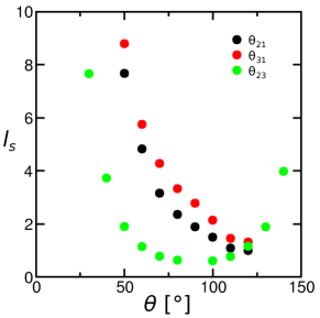
Figure 13: (Color online) Estimated slip length vs. equilibrium contact angle for the liquid-liquid and the liquid-gas interfaces.

In Fig. 13, we compare $L_{s}$ for the three interfaces, as function of the equilibrium contact angle. More specifically, for our geometry we obtain $\theta_{21}$ (receding), $\theta_{31}$ (advancing) and $\theta_{23}$ (advancing for $\theta_{23}<90^{\circ}$ and receding for $\theta_{23}>90^{\circ}$). The slip length for the liquid-liquid interface shows a minimum for $\theta_{23}=90^{\circ}$ (the data point not present, because for this combination of angles we have no net driving force $\Delta\gamma=0$) and increases symmetrically for larger and smaller angles. In contrast the slip length for the liquid-gas interfaces shows a monotonic decrease as the equilibrium contact angle increases. For the last available data point, at $\theta=120^{\circ}$, $L_{s}$ is similar for all three interfaces, while for smaller angles $L_{s}$ is significantly larger for the liquid-gas interfaces.

These results show that the slip properties in the system strongly depend on the nature of the fluid-fluid interface. In our tests the liquid-gas interfaces present a larger slip length (up to a factor 4) compared to the liquid-liquid interface, likely due to the combined effect of two distinct mechanisms operating on the density $\rho$ and the field $\phi$.

VII Discussion and conclusions

In this work we have thoroughly benchmarked our ternary high density ratio free energy model, and provided guidelines to select the free energy parameters for obtaining a wide range of surface tension combinations. We have quantified the deviations of the interface profile by measuring the “Deformation coefficient”, and systematically investigated 8 subspaces, covering relevant combinations of parameters. All data are reported in the supplementary information, including fitting functions to estimate the surface tensions.

We have compared three methods for wetting of solid boundaries, namely force, geometric extrapolation and geometric interpolation. Of the two geometric methods, geometric interpolation is significantly more accurate. The force method provides an useful alternative to geometric methods, as it does not require us to detect the fluid interface a priori, and automatically satisfies the Girifalco-Good relation, Eqn. (44).

The benchmark on the dynamics of capillary filling shows that the force method is slightly less accurate than the geometric methods. The deviations in the measured pre-factor of the Washburn law increase as the material contact angles depart from neutral wetting. Because the additional force terms also increase, we expect that the deviations are related to additional spurious velocities generated by the forcing terms. At the same time no spurious velocities are observed in the geometric methods.

Furthermore we have have performed a ternary specific benchmark, and studied the motion of self-propelled bi-slugs forming three finite and unbalanced contact angles. The analytic model for the bi-slug motion, derived by assuming equilibrium values for the contact angles, accurately captures the linear dependence of steady state velocities from the inverse of the bi-slug length, for long trains of drops and small velocities. The level-off of the velocity experimentally observed for shorter bi-slugs is captured in our simulations by accounting for the dynamic angle correction in the driving force. The agreement shows that the viscous bending of the liquid interfaces represents the main correction in the model.

Finally we have shown that coupling multiphase and multicomponent models leads to significant differences in the slip properties of liquid-liquid and liquid-gas interfaces. While for liquid-liquid interfaces the only slip mechanism is related to the diffusion of the field $\phi$, for liquid-gas interfaces the slip mechanism combines the diffusion of the field $\phi$ and the evaporation/condensation of the density $\rho$.

In our tests, at parity of interfacial properties, the slip length varies with the material contact angle and is generally larger for the liquid-gas interfaces than for the liquid-liquid interfaces. A more detailed analysis of the slip properties of the system will be the subject of a future investigation.

VIII Acknowledgement

NB gratefully acknowledges financial support from University of Northumbria at Newcastle via a Postgraduate Research Studentship. IK acknowledges support by European Research Council (ERC) Advanced Grant 834763-PonD and by Swiss National Science Foundation (SNF) grant 200021_172640. HK thanks Procter & Gamble (P&G) and EPSRC for funding (EP/P007139/1). CS acknowledges support from Northumbria University through the Vice-Chancellor’s Fellowship Programme.

References

- Wöhrwag et al. (2018) M. Wöhrwag, C. Semprebon, A. M. Moqaddam, I. Karlin, and H. Kusumaatmaja, Phys. Rev. Lett. 120, 234501 (2018), 1710.07486 .
- Utada et al. (2005) A. S. Utada, E. Lorenceau, D. R. Link, P. D. Kaplan, H. A. Stone, and D. A. Weitz, Science (New York, N.Y.) 308, 537 (2005).
- Planchette et al. (2011) C. Planchette, E. Lorenceau, and G. Brenn, Fluid Dyn. and Mat. Proc. 7, 279 (2011).
- Planchette et al. (2018) C. Planchette, S. Petit, H. Hinterbichler, and G. Brenn, Phys. Rev. Fluids 3, 093603 (2018).
- Wang et al. (2004) C. H. Wang, C. Z. Lin, W. G. Hung, W. C. Huang, and C. K. Law, Combust. Sci. Technol. 176, 71 (2004).
- Changlin-lin et al. (2013) L. Changlin-lin, L. Xin-wei, Z. Xiao-liang, L. Ning, D. Hong-na, W. Huan, and L. Yong-ge, in SPE Asia Pacific Oil and Gas Conference and Exhibition, Vol. 2 (Society of Petroleum Engineers, 2013).
- Murphy et al. (2015) D. W. Murphy, C. Li, V. D’Albignac, D. Morra, and J. Katz, J. Fluid Mech. 780, 536 (2015).
- Smith et al. (2013) J. D. Smith, R. Dhiman, S. Anand, E. Reza-Garduno, R. E. Cohen, G. H. McKinley, and K. K. Varanasi, Soft Matter 9, 1772 (2013).
- Keiser et al. (2017) A. Keiser, L. Keiser, C. Clanet, and D. Quéré, Soft Matter 13, 6981 (2017).
- Hua et al. (2014) H. Hua, J. Shin, and J. Kim, International J. Heat Fluid Flow 50, 63 (2014).
- Merriman et al. (1994) B. Merriman, J. K. Bence, and S. J. Osher, J. Comp. Phys. 112, 334 (1994).
- Gao and Feng (2011) P. Gao and J. J. Feng, J. Fluid Mech. 682, 415 (2011).
- Kim (2012) J. Kim, Comm. Comp. Phys. 12, 613 (2012).
- Zhang et al. (2016) C.-Y. Zhang, H. Ding, P. Gao, and Y. L. Wu, J. Comp. Phys. 309, 37 (2016).
- Haghani Hassan Abadi et al. (2018) R. Haghani Hassan Abadi, M. H. Rahimian, and A. Fakhari, J. Comp. Phys. 374, 668 (2018).
- Park (2018) J. M. Park, Appl. Math. Comput. 330, 11 (2018).
- Succi (2001) S. Succi, The Lattice Boltzmann equation: for fluid dynamics and beyond (Oxford University Press, 2001).
- Krüger et al. (2017) T. Krüger, H. Kusumaatmaja, A. Kuzmin, O. Shardt, G. Silva, and E. M. Viggen, The Lattice Boltzmann Equation (2017).
- Kusumaatmaja et al. (2006) H. Kusumaatmaja, J. Leopoldes, a. Dupuis, J. M. Yeomans, J. Léopoldès, a. Dupuis, and J. M. Yeomans, Europhys. Lett. (EPL) 73, 740 (2006), 0601541 .
- Kusumaatmaja and and J. M. Yeomans (2007) H. Kusumaatmaja and and J. M. Yeomans, Langmuir 23, 6019 (2007).
- Ledesma-Aguilar et al. (2011) R. Ledesma-Aguilar, R. Nistal, a. Hernández-Machado, and I. Pagonabarraga, Nature Materials 10, 367 (2011).
- Komrakova et al. (2014) A. E. Komrakova, O. Shardt, D. Eskin, and J. J. Derksen, Int. J. Multiphas. Flow 59, 24 (2014).
- Premnath and Abraham (2005) K. N. Premnath and J. Abraham, Phys. Fluids 17, 1 (2005).
- Mazloomi Moqaddam et al. (2015) A. Mazloomi Moqaddam, S. S. Chikatamarla, and I. V. Karlin, J. Stat. Phys. 161, 1420 (2015).
- Moqaddam et al. (2016) A. M. Moqaddam, S. S. Chikatamarla, and I. V. Karlin, Phys. Fluids 28 (2016).
- Montessori et al. (2017) A. Montessori, P. Prestininzi, M. La Rocca, and S. Succi, Phys. Fluids 29 (2017).
- Mukherjee and Abraham (2007) S. Mukherjee and J. Abraham, J. Colloid Interf. Sci. 312, 341 (2007).
- Lee and Liu (2010) T. Lee and L. Liu, J. Comp. Phys. 229, 8045 (2010).
- Banari et al. (2014) A. Banari, C. F. Janßen, and S. T. Grilli, Comp. Math. Appl. 68, 1819 (2014).
- Ashoke Raman et al. (2016) K. Ashoke Raman, R. K. Jaiman, T. S. Lee, and H. T. Low, Chem. Eng. Sci. 145, 181 (2016).
- Liu et al. (2015a) Y. Liu, M. Andrew, J. Li, J. M. Yeomans, and Z. Wang, Nature Communications 6, 1 (2015a), 1511.00064 .
- Andrew et al. (2017) M. Andrew, Y. Liu, and J. M. Yeomans, Langmuir 33, 7583 (2017).
- Sbragaglia et al. (2014) M. Sbragaglia, L. Biferale, G. Amati, S. Varagnolo, D. Ferraro, G. Mistura, and M. Pierno, Phys. Rev. E 89, 1 (2014).
- Mazloomi Moqaddam et al. (2017) A. Mazloomi Moqaddam, S. S. Chikatamarla, and I. V. Karlin, J. Fluid Mech. 824, 866 (2017), 1608.03208 .
- Travasso et al. (2005) R. D. M. Travasso, G. A. Buxton, O. Kuksenok, K. Good, and A. C. Balazs, J. Chem. Phys. 122, 5 (2005).
- Spencer et al. (2010) T. J. Spencer, I. Halliday, and C. M. Care, Phys. Rev. E 82, 066701 (2010).
- Ridl and Wagner (2018) K. S. Ridl and A. J. Wagner, Phys. Rev. E 98, 1 (2018), 1805.07251 .
- Semprebon et al. (2016) C. Semprebon, T. Krüger, and H. Kusumaatmaja, Phys. Rev. E 93, 033305 (2016).
- Semprebon et al. (2017) C. Semprebon, G. McHale, and H. Kusumaatmaja, Soft Matter 13, 101 (2017), 1604.05362 .
- Sadullah et al. (2018) M. S. Sadullah, C. Semprebon, and H. Kusumaatmaja, Langmuir 34, 8112 (2018).
- Mazloomi M et al. (2015) A. Mazloomi M, S. S. Chikatamarla, and I. V. Karlin, Phys. Rev. Lett. 114, 174502 (2015).
- Liang et al. (2019) H. Liang, J. Xu, J. Chen, Z. Chai, and B. Shi, App. Math. Mod. , 1 (2019), 1710.09534 .
- Shi et al. (2016) Y. Shi, G. H. Tang, and Y. Wang, J. Comp. Phys. 314, 228 (2016).
- Wang et al. (2015) Y. Wang, C. Shu, H. B. Huang, and C. J. Teo, J. Comp. Phys. 280, 404 (2015).
- Chikatamarla et al. (2006) S. S. Chikatamarla, S. Ansumali, and I. V. Karlin, Phys. Rev. Lett. 97, 1 (2006).
- Yuan and Schaefer (2006) P. Yuan and L. Schaefer, Phys. Fluids 18, 1 (2006).
- Mazloomi M. et al. (2015) A. Mazloomi M., S. S. Chikatamarla, and I. V. Karlin, Phys. Rev. E 92, 023308 (2015).
- Karlin et al. (1999) I. V. Karlin, A. Ferrante, and H. C. Öttinger, Europhys. Lett. (EPL) 47, 182 (1999).
- Ansumali et al. (2003) S. Ansumali, I. V. Karlin, and H. C. Öttinger, Europhys. Lett. 63, 798 (2003), 0205510v2 .
- Briant and Yeomans (2004) A. J. Briant and J. M. Yeomans, Phys. Rev. E 69, 031603 (2004).
- Briant et al. (2004) A. J. Briant, a. J. Wagner, and J. M. Yeomans, Phys. Rev. E 69, 031602 (2004), 0203093 .
- Ladd (1994) A. J. C. Ladd, J. Fluid Mech. 271, 285 (1994), 9306005 .
- Huang et al. (2007) H. Huang, D. T. Thorne, M. G. Schaap, and M. C. Sukop, Phys. Rev. E 76, 1 (2007).
- Girifalco and Good (1957) L. Girifalco and R. Good, J. Phys. Chem. 61, 904 (1957).
- Ding and Spelt (2007) H. Ding and P. D. M. Spelt, Phys. Rev. E 75, 1 (2007).
- Lee and Kim (2011) H. G. Lee and J. Kim, Comp. Fluids 44, 178 (2011).
- Lucas (1918) R. Lucas, Kolloid-Zeitschrift 23, 15 (1918).
- Washburn (1921) E. W. Washburn, Phys. Rev. 17, 273 (1921).
- Wiklund et al. (2011) H. S. Wiklund, S. B. Lindström, and T. Uesaka, Computer Physics Communications 182, 2192 (2011).
- Liu et al. (2015b) H. Liu, Y. Ju, N. Wang, G. Xi, and Y. Zhang, Phys. Rev. E 92, 1 (2015b).
- Lou et al. (2018) Q. Lou, M. Yang, and H. Xu, Comm. Comp. Phys. 23, 1116 (2018).
- Diotallevi et al. (2009) F. Diotallevi, L. Biferale, S. Chibbaro, A. Lamura, G. Pontrelli, M. Sbragaglia, S. Succi, and F. Toschi, Europ. Phys. J: Special Topics 166, 111 (2009).
- Esmaili et al. (2012) E. Esmaili, A. Moosavi, and A. Mazloomi, J. Stat. Mech. 2012 (2012).
- Huang et al. (2014) J.-J. Huang, H. Huang, and X. Wang, Phys. Fluids 26, 062101 (2014).
- Bico and Quéré (2000) J. Bico and D. Quéré, Europhys. Lett. 51, 546 (2000).
- Bico and Quéré (2002) J. Bico and D. Quéré, J. Fluid Mech. 467, 101 (2002).
- Kusumaatmaja et al. (2016) H. Kusumaatmaja, E. J. Hemingway, and S. M. Fielding, J. Fluid Mech. 788, 209 (2016), 1507.08945 .
- JACQMIN (2000) D. JACQMIN, J. Fluid Mech. 402, S0022112099006874 (2000).
- Cox (1986) R. G. Cox, J. Fluid Mech. 168, 195 (1986).
- Cox (1998) R. G. Cox, J. Fluid Mech. 357, 249 (1998).