The Higgs Profile in the Standard Model and Beyond

Abstract

We present a review of Higgs physics in the SM and beyond, including the tests of the Higgs boson properties that have been performed at LHC and have permitted to delineate its profile. After presenting the essential features of the Brout-Englert-Higgs (BEH) mechanism, and its implementation in the SM, we discuss how the Higgs mass limits developed over the years. These constraints in turn helped to classify the Higgs phenomenology (decays and production mechanisms), which provided the right direction to search for the Higgs particle, an enterprise that culminated with its discovery at LHC. So far, the constraints on the couplings of the Higgs particle, point towards a SM interpretation. However, the SM has open ends that suggest the need to look for extensions of the model. We discuss in general the connection of the Higgs sector with some new physics (e.g. supersymmetry, flavor and Dark matter), with special focus on a more flavored Higgs sector. Thus is realized in the most general 2HDM, and its textured version, which we study in general, and for its various limits, which contain distinctive flavor-violating signals that could be searched at current and future colliders.

I Introduction

The discovery of the Higgs boson, announced on July 4th by the CERN LHC collaborations higgs-atlas:2012gk ; higgs-cms:2012gu , marked the completion of our current theory of the fundamental particles and their interactions, the so-called Standard Model (SM) Glashow:1961tr ; Weinberg:1967tq ; Salam:1968rm . This event can be considered one of the greatest accomplishments of the High Energy Physics community and knowing how it was made possible, as well as the implications, should become part of the culture of particle physics. This is precisely the purpose of this review paper.

The search for an understanding of the structure of matter and its interactions, has been a moto of the physical sciences, which could be traced back to the early days of modern atomic theory. After the establishment of quantum mechanics and its application to atomic and nuclear systems, relativist quantum fields made its appearance and allowed to formulate a consistent quantum theory for electrons and photons, quantum electrodynamics (QED), which successfully predicted antimatter (positrons for the electron). Afterwards, particle physics passed through great times in the 50-60’s, when plenty of data was collected by the experimental collaborations from high-energy labs around the world. This branch of physics advanced by the detection of a rich spectrum of new strongly interacting resonances, the hadrons. However, it was not known whether quantum field theory (QFT) would survive or not, as the correct description of particles and interactions. More general approaches, such as dual models, saw the light just to be shown years later to be a different guise for same good old QFT.

Progress was also made on the description of Weak interactions, which move from the Fermi 4-fermion effective theory of beta decay, to the Intermediate Vector Boson theory. Promising quantum unified theories were formulated, which included non-abelian symmetries that contained self-interacting gauge bosons. These theories seemed to work only for massless gauge fields, as the photon of QED, but in the case of weak interactions it was needed to consider massive gauge bosons (such as the charged $W^{\pm}$ that was supposed to mediate the weak interactions).

Two lines of work were undertaken, one of them attempted to find some consistent way to make the Yang Mills fields massive, independently of a realistic model. Following the ideas of Nambu on spontaneous symmetry breaking, a solution to this problem appeared with the initial formulation of the Brout-Englert-Higgs (BEH) mechanism Higgs:1964pj ; Englert:1964et ; Guralnik:1964eu , which was shown to be a viable mechanism to generate the masses of the elementary particles (gauge bosons and chiral fermions). This mechanism was incorporated within the unified Electroweak (EW) gauge model Glashow:1961tr ; Weinberg:1967tq ; Salam:1968rm . From the model building perspective, the electroweak SM was completed after the Glashow-Iliopoulos-Maiani mechanism was proposed Glashow:1970gm , which received further confirmation with the detection of the charm quark. The strong interactions were described by a gauge theory too, quantun chromodynamics (QCD), where quarks bind into hadrons through interactions mediated by gluons.

The other line involved a detailed study of the renormalization problem associated with having massive gauge bosons, with M. Veltman acting as the driving force behind this project Veltman:1968ki . Nowadays, we know that the SM is a renormalizable Quantum Field Theory (QFT), that is quite successfull in describing the interactions of the fundamental particles. The detection of the W and Z in the 80’s at CERN, and jet events initiated by gluons at DESY, brought extra confirmation of the SM.

The Higgs boson was recognized as a testable sector the SM in the mid 70’s and early 80’s, when the first papers discussed the methods to search for direct effects of the Higgs boson in particle accelerators Ellis:1975ap ; Georgi:1977gs ; Glashow:1978ab , and this was complemented by the study of indirect Higgs effects (Radiative corrections) on the properties of the SM particles and its related parameters Veltman:1977fy .

Given the success of the SM, it became credible that all interactions could be unified in a single gauge group. Construction of experimental facilities to search for proton decay were started in the early 80’s, but since no proton decay was observed, the unification paradigm loosed some momentum. At that time a concrete Supersymmetric (SUSY) extension of the SM was proposed too, which was shown to ameliorated the hierarchy/naturalness problem of the Higgs mass.

This is more or less the time when the author entered into graduate school, at the University of Michigan, and continued studying the Higgs particle. The community was engaged in a debate about the best options for constructing of next colliders, and there were discussions about the best strategy to produce and detect the Higgs particle, although many efforts were devoted to build models that did not require an elementary scalar, the technicolor adventure. Given the success of the hadron machine that made possible to detect the W and Z bosons, it seemed that the best strategy for a high energy collider, was the proton-proton or proton-antiproton choices. The USA made plans to study the Higgs particle, and other forms of new physics, at a proton-proton collider, the SSC, that was designed to work with c.m. energy of 40 TeV. Tevatron (a proton-antiproton collider) was also approved, with c.m. energy of 1.8 TeV, which was thought to be good enough to produce and detect the top quark. But this was the mid 80’s, and CERN had planned to build a circular electron-positron collider that would work first at the Z pole (LEPI) and then above the WW threshold (LEPII).

The reason why such high energy was considered for SSC, was in part due to the lack of knowledge of the Higgs mass. At U of Michigan, a series of talks were planned for the fall of 87 to discuss the search for the Higgs boson. First talk was by Tiny Veltman, who argued that the best way to start getting information on the Higgs mass was from a detailed analysis of radiative corrections, which years later proved to be very useful to constrain the Higgs mass. The second talk was by Gordy Kane, who presented the different techniques that should be used to search for a Higgs particle at a hadron collider. In those days the Higgs mass ($m_{h}$) was classified into several ranges: light ($m_{h}\leq m_{Z}$), intermediate ($m_{Z}\leq m_{h}\leq 2m_{t}$) and heavy $2m_{t}\leq m_{h}\leq 600$ GeV). Considering these mass ranges made sense at that time, because it was thought that the top mass should be close to the value of 45 GeV, as was claimed early on by C. Rubbia at CERN. As the Tevatron entered into the game, the lower limits on the top mass started to increase, and together with results from B-physics, it was suspected that $m_{t}$ was above 90 GeV. Until it was detected at Tevatron in the mid 90’s with mass $m_{t}\simeq 175$ GeV, and then the intermediate Higgs mass range was redefined as $m_{Z}\leq m_{h}\leq 2m_{Z}$.

A light Higgs could have been detected using the associated production of the Higgs with a gauge boson, with the Higgs decaying into bb pairs. In fact, such range was the task of the LEP collider at CERN. The most difficult task, as Kane argued, was the above mentioned intermediate mass range. After we learned that top was heavier than $m_{Z}$, the intermediate mass range was redefined, and its associated difficulties disappeared from Higgs hunting considerations, but the techniques that were devised by Kane et al, proved to be very useful in the ultimate search at LHC that provided first hints of the Higgs particle in 2012. Heavy higgs could had been detected in the golden mode $h\to ZZ$, until the Higgs mass was so large that a perturbative treatment would no longer be reliable. Such range was termed the obese mass region, starting from about 600 GeV. The third talk of the series was presented by an experimentalist, R. Thun, who discussed the issue of the signal vs backgrounds, with some estimated characteristics for semi-realistic detectors, and he showed that both theoretical works would be very difficult to realize at planned colliders.

The 90’s witnessed the entering of operation of LEP II, with cm energy of 200 GeV. The search for Higgs at LEP used the reaction $e^{+}e^{-}\to h+Z$, and resulted in successive bounds on Higgs mass, which eventually reached the value $m_{h}\geq 111$ GeV at the end of LEP life-time. The tail of a Higgs signal was believed to had been observed at the final stages of LEP, which ignited some pressure to keep LEP running, but the director say no, which was in fact a good choice, and the tunnel was cleaned to start the installation of LHC magnets and the construction of the giant detectors ATLAS and CMS. These detectors were designed to catch a Higgs boson in the narrow mass range left by the analysis of electroweak precision tests, namely $115\leq m_{h}\leq 130$ GeV, which could be probed with the modes $h\to\gamma\gamma$ and $h\to ZZ$ that were studied early on by Kane et al .

LHC started taking data on 2011, but nothing really big came out of those early runs apart from some fake signals and rumors. The big news have to wait until mid 2012, when the LHC announced the discovery of a Higgs-like particle with $m_{h}=125-126$ GeV at the LHC higgs-atlas:2012gk ; higgs-cms:2012gu , a landmark event that provided a definite test of the mechanism of Electro-Weak symmetry breaking Gunion:1989we . Thus, after many years of hypothesis and conjectures, it was finally possible to confirm that ”what we thought about the origin of masses and Higgs mechanism, is real …” kane .

The Higgs mass value agrees quite well with the range preferred by the electroweak precision tests (EWPT) Erler:2007sc , which confirms the success of the SM. Current measurements of its spin, parity, and couplings, also seem consistent with the SM. The fact that LHC has verified the linear realization of spontaneous symmetry breaking (SSB), as included in the Standard Model (SM), could also be taken as an indication that Nature likes scalars.

The initial reports from LHC claimed the discovery of a resonance with mass $m=125-126$ GeV, through its decays into $\gamma\gamma$ and $ZZ^{*}$, which were consistent with having either spin $s=0$ or $s=2$. Later on, with more data collected from more decay modes, it was concluded that the simplest choice $s=0$ was favored. After LHC delivered the Higgs signal, many papers have been devoted to study the Higgs couplings, and the constraints on deviations from SM Espinosa:2012im ; Cheung:2013rva ; Ellis:2014dva . Although the initial data showed also some tantalizing hints of deviations from the SM predictions, including first a possible enhanced $\gamma\gamma$ rate, and later on a signal from the LFV Higgs decay modes appeared to had been detected, these signals were not confirmed with more data. So far, we can say that the signal resembles a Higgs scalar, with a profile consistent with the SM interpretation.

On the other hand, the LHC has also been searching for signals of Physics Beyond the SM, which has been conjectured in order to address some of the problems left open by the SM, such as hierarchy, flavor, unification, etc Arkani-Hamed:2016kpz . Some of these extensions of the SM, such as SUSY and multi-Higgs models in general Accomando:2006ga , predict deviations from the SM Higgs couplings, while at the same time contain a rich Higgs spectrum, whose detection would be a clear signal of new physics.

However, the LHC has provided bounds on the new physics scale ($\Lambda$), that are already entering into the multi-TeV range, and this is casting some doubts about the theoretical motivations for new physics scenarios with a mass scale of order TeV. This is particularly disturbing for the concept of naturalness, and its supersymmetric implementation, since the bounds on the mass of superpartners are passing the TeV limit too. However, some of the motivations for new physics are so deep, that it seems reasonable to wait for the next LHC runs, with higher energy and luminosity, in order to have stronger limits, both on the search for new particles, such as heavier Higgs bosons, and for precision tests of the SM properties.

This review paper is intended to cover the essential of Higgs physics, starting with a quick review of the SM Higgs, then looking at the motivations for some extensions of the Higgs sector, and focusing then in the most general Two-Higgs doublet model (2HDM). We hope our paper complements the excellent reviews on Higgs physics that have appeared recently Altarelli:2013lla ; Ellis:2015tba ; Haber:2017udj ; Dawson:2018dcd ; Kane:2018oax ; Wells:2018nwj . The organization of our paper goes as follows. We shall present in Section 2, the SM Higgs Lagrangian, including the Higgs potential, the gauge and Yukawa interactions, as well as the theoretical constraints on the Higgs mass. We start section 3 with discussion of the Higgs couplings with gauge bosons and fermions, first within the SM and then presenting a model-independent approach; this parametrization is proposed to describe Higgs couplings that include flavor and Charge-conjugation Parity (CP) violation. Then, we discuss briefly the Higgs phenomenology at the LHC, which allowed to gather information and draw the current Higgs boson profile. Although the Higgs properties could be discussed within an effective Lagrangian approach, it is also important to discuss them within an specific model, where such deviations could be interpreted and given a context. Thus, in section 4 we discuss the motivation for extending the SM Higgs sector, with a focus on the multi-Higgs models, including its Supersymmetric versions and models with Higgs-Flavon mixing; some remarks on the Higgs portal and its dark matter (DM) connection is presented too. Section 5 contains a detailed discussion of one of such models where one has a ”more flavored Higgs sector”, namely the most general two-Higgs doublet model (the 2HDM of type III and its textured realization), which includes new sources of flavor and CP violation. As phenomenological predictions we discuss the Lepton Flavor Violating (LFV) Higgs decays $H_{i}\to l_{i}l_{j}$ and the top quark Flavor-Changing-Neutral-Currents (FCNC) transitions $t\to ch$ Hou:1991un . Concluding remarks are included in section 6, where we end with a brief discussion about possible paths for the future, including some comments about the options to tests of the Higgs couplings with light quarks, which in turn take us to consider the so called ”private” Higgs models.

II SM Higgs Lagrangian: Gauge and Yukawa couplings

After many years of theoretical and experimental efforts, we have now a great theory of the elementary constituents of nature and its fundamental interactions, the Standard Model (SM), which is based on the following (For recet texts see: Lancaster:2014pza ; Schwartz:2013pla ):

• The fundamental particles are the quarks and leptons, which appear repeated in three chiral families. Quarks form the hadrons, such as the proton, neutron, pions, etc. Charged leptons, such as electron, muon and tau, are accompanied by the light neutrinos.

• The quarks and leptons have interactions that follow from the Gauge principle, i.e. the forces are mediated by vector particles associated with gauge symmetries, and there is one gauge field for each generator of the Lie algebras associated with the symmetries of the system.

• The masses of the weak gauge bosons ($W^{\pm},Z$), and the fermions, arise as a consequence of the interactions of the particles with the vacuum, which can live in a broken phase, i.e. the BEH mechanism.

The BEH mechanism, was implemented by Weinberg in the model proposed by Glashow, which was based on the gauge group $SU(2)_{L}\times U(1)_{Y}$. Treating quarks and leptons as the fundamental degrees of freedom, lead to the correct formulation of the SM. We shall start by presenting the essential features of the SM and the BEH mechanism.

II.1 SM gauge and fermion sector

The weak and electromagnetic interactions are partly unified into the Electroweak theory, which has the gauge symmetry $SU(2)_{L}\times U(1)_{Y}$. The Lagrangian for the gauge and fermion sector (leptons) is given by:

$${\cal{L}}=\bar{L}{\gamma}^{\mu}D_{\mu}L+\bar{e}_{R}{\gamma}^{\mu}D^{\prime}_{\mu}e_{R}-\frac{1}{4}W^{\mu\nu i}W_{\mu\nu}^{i}-\frac{1}{4}B^{\mu\nu}B_{\mu\nu},$$ (1)

where

$$D_{\mu} =\partial_{\mu}+i\frac{g}{2}\sigma^{i}W_{\mu}^{i}+i\frac{g^{\prime}}{2}B_{\mu},$$ (2)

$$D^{\prime}_{\mu} =\partial_{\mu}+ig^{\prime}B_{\mu},$$ (3)

Here $L$ denotes the left-handed lepton doublet, while $e_{R}$ corresponds to the right-handed electron, $\sigma^{i}$ are the Pauli matrices and $g$ y $g^{\prime}$ denote the gauge coupling constants. The tensors $W_{\mu\nu}^{i}$ and $B_{\mu\nu}$ are given by:

$$W_{\mu\nu}^{i} =\partial_{\mu}W_{\nu}^{i}-\partial_{\nu}W_{\mu}^{i}-g\epsilon^{ijk}W_{\mu}^{j}W_{\nu}^{k},$$ (4)

$$B_{\mu\nu} =\partial_{\mu}B_{\nu}-\partial_{\nu}B_{\mu}.$$ (5)

In addition we need to include the quarks, with the left-handed components forming a doublet of weak isospin, while the right-handed ones transform as singlets. Quarks are also triplets of the color interactions, which is described by the gauge symmetry $SU(3)_{c}$. Thus, the full SM gauge symmetry is: $SU(3)_{c}\times SU(2)_{L}\times U(1)_{Y}$.

II.2 SSB and the Higgs

Insights from the role of the vacuum in condensed matter, helped to identify how a symmetry is realized in QFT, namely:

• A symmetry is realized a la Wigner-Weyl, when the vacuum respects such symmetry, i.e. the minimum of the energy happens for vanishing field variables, as in QED where $<A^{\mu}>=0$.

• A realization a la Nambu-Goldstone occurs when the vacuum does not respect the symmetry of the Lagrangian, which leads to Goldstone Theorem: When a Global symmetry is broken spontaneously (SSB), massless particles associated with the broken generators appear.

SSB happens for instance in strong interactions, where the Chiral symmetry is not manifest, and the pions are identified as pseudo Nambu-Goldstone bosons (NGB) (pseudo means they are not exactly NGB, due to the small mass of the light quarks ($u,d,s$)).

In the case of the weak interactions, the problem was how to include the mass for the charged W bosons, the mediators of the weak interactions that manifest in neutron beta decay. The solution came with the BEH mechanism Englert:1964et ; Higgs:1964pj ; Guralnik:1964eu , which proved that within the context of a local symmetry, the degrees of freedom associated with the Goldstone bosons become the longitudinal modes of the gauge bosons, which then acquire a mass.

Let us discuss this mechanism for a simple Abelian theory, with Lagrangian:

$${\cal{L}}_{\phi}=\frac{1}{2}\partial_{\mu}\phi\partial^{\mu}\phi-V(\phi),\hskip 14.22636ptV(\phi)=\frac{1}{2}\mu^{2}\phi^{2}+\frac{1}{4}\lambda\phi^{4}$$ (6)

where $\lambda>0$.

This Lagrangian (6) is invariant under the parity (P) transformation $\phi\to-\phi$. However, when one minimizes the potential, we find that:

• (a) For $\mu^{2}>0$, the minimum is invariant under P, and it occurs for:

  $$\langle\phi\rangle_{0}=\langle 0|\phi|0\rangle=0.$$ (7)

• (b) For $\mu^{2}<0$, the minimum is displaced from the origin, and does not respect P, i.e.

  $$\langle\phi\rangle_{0}=\pm\sqrt{\frac{-\mu^{2}}{2\lambda}}\equiv\pm\frac{v}{\sqrt{2}}.$$ (8)

Now, there is a degeneracy between $v$ y $-v$. Then, one can study the fluctuations around the new minimum, which are interpreted as the particles, i.e. $\xi(x)\equiv\phi(x)-\langle\phi\rangle_{0}=\phi(x)-v$.

Then, the Lagrangian for the field $\xi$ (the fluctuation) becomes:

$${\cal{L}}_{\xi}=\frac{1}{2}\partial_{\mu}\xi\partial^{\mu}\xi-\lambda v^{2}\xi^{2}-\lambda v\xi^{3}-\frac{1}{4}\lambda\xi^{4}.$$ (9)

Thanks to SSB, this Lagrangian contains now a scalar field $\xi$ with mass $m_{\xi}=\sqrt{2\lambda}v=\sqrt{-2\mu^{2}}$. When one uses SSB within the context of a gauge theory, it is possible to generate masses for the gauge bosons.

Within the SM the gauge symmetry for the electroweak interactions is $SU(2)\times U(1)_{Y}$, with gauge bosons $W^{\pm}_{\mu},W^{3}_{\mu}$ and $B_{\mu}$. The minimal Higgs sector includes one Higgs doublet, which can be written as follows:

$$\Phi=\frac{1}{\sqrt{2}}\begin{bmatrix}\phi_{1}-i\phi_{2}\\ \phi_{3}-i\phi_{4}\end{bmatrix}.$$ (10)

The mass terms for the $W,Z$ is obtained from the the Higgs Lagrangian, which includes the Higgs kinetic term, its gauge interactions, and the Higgs potential, i.e.

$${\cal{L}}_{H}=|D_{\mu}\Phi|^{2}-V(\Phi),$$ (11)

The potential $V(\Phi)$ is written as:

$$V(\Phi) = \mu^{2}\Phi^{\dagger}\Phi+\lambda\left(\Phi^{\dagger}\Phi\right)^{2}$$ (12)

$$= \frac{1}{2}\mu^{2}\left(\sum_{j=1}^{4}\phi_{i}^{2}\right)+\frac{1}{4}\lambda\left(\sum_{j=1}^{4}\phi_{i}^{2}\right)^{2}.$$

For $\mu^{2}<0$, the gauge symmetry $SU(2)_{L}\times U(1)_{Y}$ is broken to $U(1)_{em}$. This is illustrated in figure 1, where we can see the different options for the vev (red points), we also display the 3-dimensional image of the potential, i.e. the mexican hat potential. In this case, part of the scalar degrees of freedom from the doublet, the so-called pseudo Goldstone bosons (pGB), become the longitudinal modes of the $W^{\pm}$ and $Z$, which then become massive. The charged pGB is identified as: $G^{\pm}=\frac{1}{\sqrt{2}}(\phi_{1}\pm i\phi_{2})$, while the neutral pGB correspond to: $G^{0}=\phi_{4}$. The remaining degree of freedom ($\phi_{3}$) includes a physical d.o.f., which by itself ”forms an incomplete scalar multiplet”, as Higgs pointed out in his classic paper Higgs:1964pj .

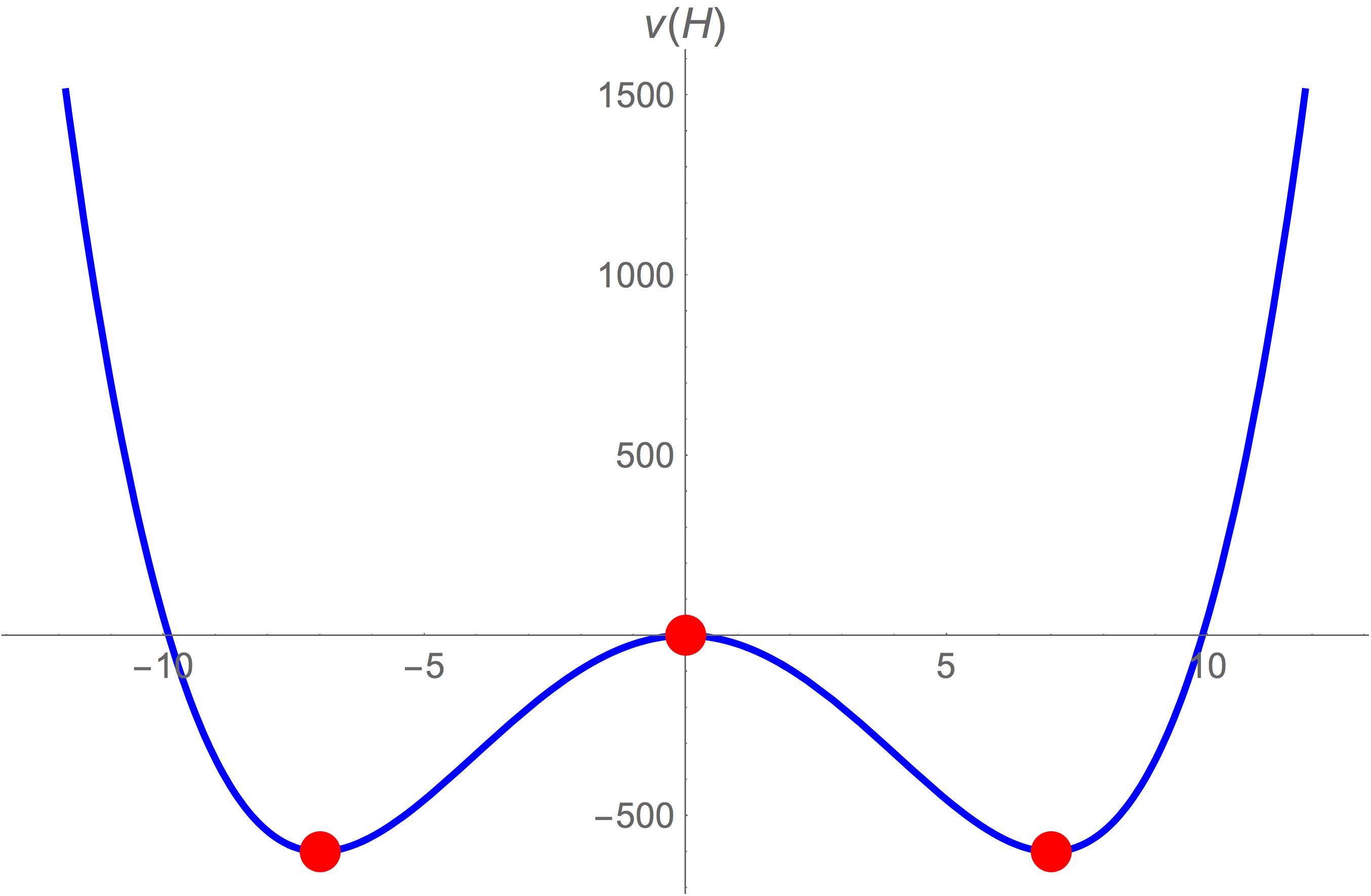
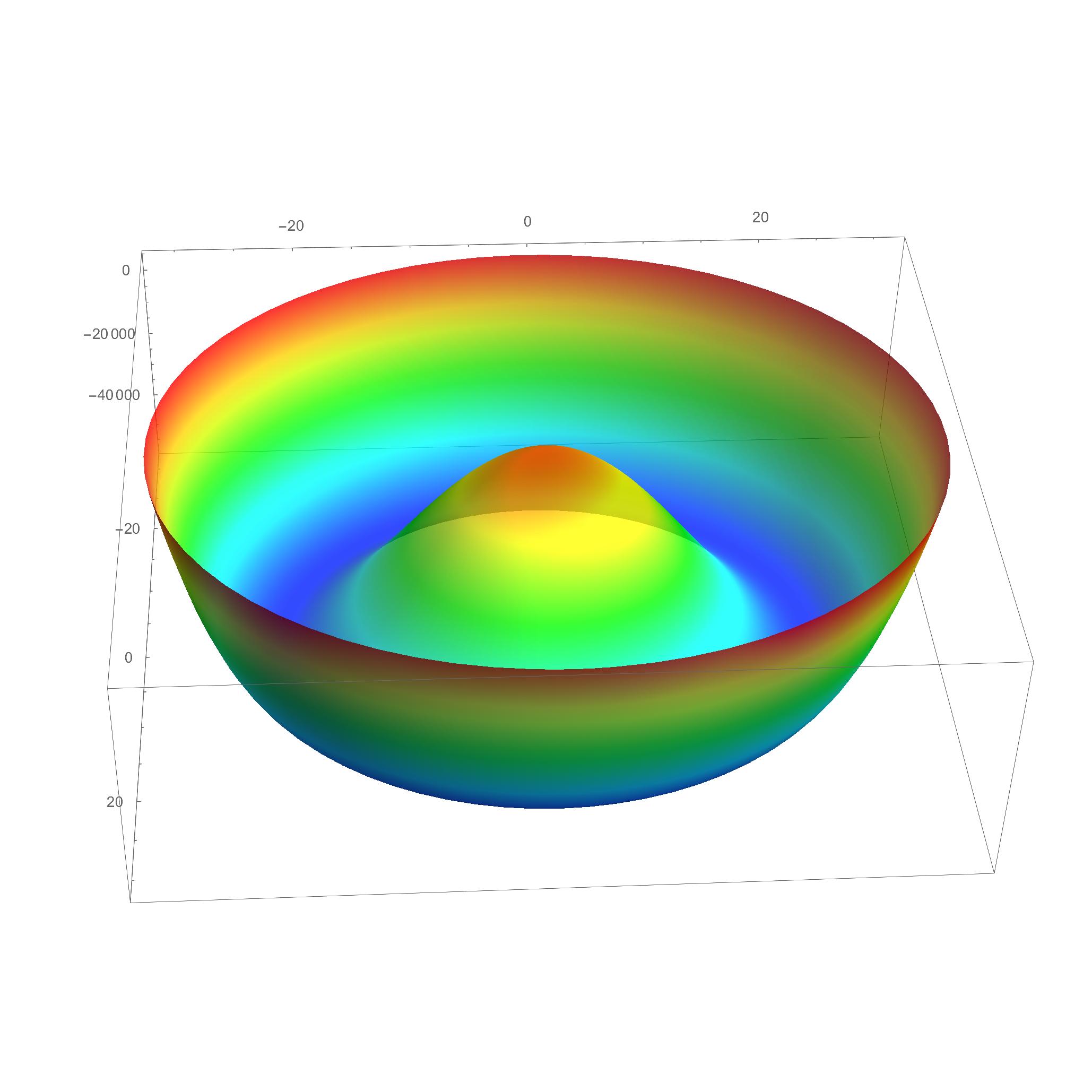
Figure 1: The Higgs potential when SSB occurs (left), and the 3-dimensional image, i.e. the mexican hat potential (right).

However, the gauge symmetry leaves us some freedom to remove non-physical degrees of freedom. This is done in the so called Unitary gauge, where one can take: $\phi_{1}=\phi_{2}=\phi_{4}=0$ y $\phi_{3}=v+h$; and $h$ corresponds to the excitations from the vev. Thus, the Higgs doublet $\Phi$ can be written in the unitary gauge as:

$$\phi=\frac{1}{\sqrt{2}}\begin{bmatrix}0\\ v+h\end{bmatrix},$$ (13)

Then, the potential $V(\phi)$ becomes:

$$V=\frac{1}{4}\lambda v^{4}+\lambda v^{2}h^{2}+\lambda vh^{3}+\frac{1}{4}\lambda h^{4}.$$ (14)

The second term in the potential (quadratic in h) indicates that the Higgs ($h$) mass is $m_{h}^{2}=2v^{2}\lambda$. The cubic and quartic terms ($h^{3},h^{4}$) describe the 3- and 4-point Higgs self-couplings.

On the other hand, the interaction of the Higgs with the gauge bosons, is contained in the kinetic term, which can be written as:

$$\bigg{|}\left(i\frac{g}{2}\sigma^{i}W_{\mu}^{i}+i\frac{g^{\prime}}{2}B_{\mu}\right)\Phi\bigg{|}^{2}=\frac{(v+h)^{2}}{8}\left(g^{2}(W^{1}_{\mu})^{2}+g^{2}(W^{2}_{\mu})^{2}+(-gW^{3}_{\mu}+g^{\prime}B_{\mu})^{2}\right).$$ (15)

We define new vector fields:

$$Z_{\mu}^{0} =\frac{1}{\sqrt{g^{2}+g^{\prime 2}}}(gW^{3}_{\mu}-g^{\prime}B_{\mu}),$$ (16)

$$W_{\mu}^{\pm} =\frac{1}{\sqrt{2}}(W_{\mu}^{1}\pm iW_{\mu}^{2}),$$ (17)

$$A_{\mu}^{\pm} =\frac{1}{\sqrt{g^{2}+g^{\prime 2}}}(g^{\prime}W^{3}_{\mu}+gB_{\mu}),$$ (18)

Thus, the Lagrangian (15) contains mass terms for these fields, i.e. $M_{W}^{2}W_{\mu}^{+}W^{-\mu}+\frac{1}{2}M_{Z}^{2}Z_{\mu}Z^{\mu}$. The corresponding masses given by $M_{W}=\frac{vg}{2},\hskip 11.38092ptM_{Z}=\frac{v}{2}\sqrt{g^{2}+g^{\prime 2}}$, while the photon remains massless, i.e. $M_{A}=0$.

We can also express the electric charge ($e$) in terms of the gauge couplings $g$ y $g^{\prime}$, as follows: $e=\frac{gg^{\prime}}{\sqrt{g^{2}+g^{\prime 2}}}=g\sin\theta_{W}$, where $\theta_{W}$ denotes the weak mixing angle. Within the SM, there holds a relationship between the gauge boson masses, which turns out to be of crucial importance, i.e. $M_{W}=M_{Z}\cos\theta_{W}$, with $\cos\theta_{W}=\frac{g}{\sqrt{g^{2}+g^{\prime 2}}}$ and $\sin\theta_{W}=\frac{g^{\prime}}{\sqrt{g^{2}+g^{\prime 2}}}$. Finally, one can also expres the Fermi constant as: $G_{F}=\sqrt{2}\frac{g^{2}}{8M_{W}^{2}}=\frac{\sqrt{2}}{2v^{2}}$.

The numerical value of the fermi constant is: $G_{F}=1.16637\times 10^{-5}GeV^{-2}$ PDG , which implies: $v\sim 246$ GeV, this value is known as the Electroweak scale. One can check that the interactions of the type $hVV$ and $hhVV$ are contained in this Lagrangian, namely:

$${\cal{L}}_{hVV}=gM_{W}hW_{\mu}^{+}W^{-\mu}+\frac{gM_{Z}}{2c_{W}}hZ_{\mu}Z^{\mu},$$ (19)

In the SM, the fermions are chiral fields, i.e. the left and right-handed fermions transform differently under the gauge symmetry, and therefore they should be massless. However, a miracle happens here: the Higgs mechanism with a minimal Higgs doublet induces the mass for the SM fermions too. Fermion masses are obtained from the Yukawa Lagrangian that includes the coupling of the fermion doublet $F_{L}$ with the Higgs doublet $(\Phi)$ and the right-handed fermion singlet $f_{R}$, which for the leptons and quarks take the form:

$${\cal{L}}_{Yukawa}=y_{e}\bar{L}\phi e_{R}+y_{d}\bar{Q}_{L}\phi d_{R}+y_{u}\bar{Q}_{L}(i\sigma_{2}\phi^{*})u_{R}+h.c.$$ (20)

After SSB, all the SM fermions acquire masses (except the neutrinos), which is given by: $m_{f}=y_{f}\frac{v}{2}$. The Yukawa Lagrangian includes the Higgs-fermion interactions too, which turn out to be proportional to the fermion mass, i.e. $(hff)=\frac{m_{f}}{v}$.

II.3 SM Higgs parameters: LEP and indirect constraints

Within the SM, the Higgs sector includes only two parameters: the (dimensional) quadratic mass term $\mu^{2}$ and the dimensionless quartic coupling $\lambda$. Once SSB is implemented, these parameters can be traded by the Higgs vev ($v$) and the Higgs mass ($m_{h}$). But what to expect for $\lambda$? Over the years, a cocktail of arguments was developed that helped to constrain the Higgs mass, namely.

• Unitarity: The processes involving gauge bosons and the Higgs, such as $WW$ scattering, should satisfy the unitarity bounds, which also translate into a Higgs mass bound of $O(1)$ TeV Lee:1977eg ; Chanowitz:1978uj , unless the Higgs interactions become strong.

• Perturbativity: Given that the EW gauge sector is weakly-interacting, one would expect that the Higgs interactions should also be weak, which would imply: $\lambda\simeq O(1)$, and then the Higgs mass was to be expected to be of order of the electroweak scale, i.e. $m_{h}=O(v)$ Cabibbo:1979ay ; Lindner:1985uk .

• Vaccum stability: A lower bound on the Higgs mass was also derived from requiring that the radiative corrections do not make the potential to develop instabilities, but this one was quickly overcome after LEP bounds on the Higgs mass..

• Radiative corrections: It is also possible to derive constraints on the Higgs mass by considering the indirect effects of the Higgs on the EW observables. This could be done by using only the corrections to the $\rho$ parameter, as it was pioneered by Veltman Veltman:1977fy . With the precision reached at LEP (and Tevatron) it was possible to refine this analysis and use the complete set of precision tests, up to the point that it was known that the Higgs mass should be at the reach of LHC.

A graphic summary of these constraints was presented in ref. Kolda:2000wi , which we show in figure 2 (left). Thus, already by 2000, it was known that the favored Higgs mass range was $110<m_{h}<180$ GeV. Fig. 2 (right), from ref. Erler:2000cr , shows that the probability distribution for the Higgs mass, which is constrained by radiative corrections to lay in the range $110<m_{h}<130$ GeV.

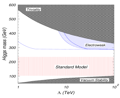
Figure 2: Higgs mass limts from theoretical considerations (left) and EWPT (right) . Figure 2- -left is from Kolda:2000wi , and figure 2-right is from Erler:2000cr

III Higgs phenomenology and the LHC

As good as it can be, the theoretical bounds on the Higgs mass, including the analysis of radiative corrections, only provided indirect tests of the Higgs mass. To prove the existence of the Higgs particle, one must produce it through some reaction at some accelerator and to detect its decay products in the particle detectors; this task started at LEP, continued at the Tevatron and finally it was completed at the LHC. The starting point for such analysis is to have the Feynman rules of the Higgs sector, which comes next.

III.1 General Couplings and Feynman rules

As mentioned in the introduction, in order to study the Higgs properties at the LHC it is both instructive and useful to present a parametrization of the Higgs couplings that is general enough, while at the same time it makes easy to reduce to the expressions to the SM limit, or some other popular SM extension, such as the 2HDM.

Thus, we shall start by describing the coupling of the scalar boson ($h$) with Vector bosons $W^{\pm},\,Z$. In this case we can write the interaction Lagrangian with terms of dimension-4, consistent with Lorentz symmetry and derivable from a renormalizable model, as follows:

$${\cal{L}}_{V}=\kappa_{W}gm_{W}hW^{+\mu}W^{-}_{\mu}+\kappa_{Z}\frac{gm_{Z}}{2c_{W}}hZ^{\mu}Z_{\mu}$$ (21)

When the Higgs particle corresponds to the minimal SM, one has $\kappa_{W}=\kappa_{Z}=1$, while values $\kappa_{W}=\kappa_{Z}\neq 1$ arise in models with several Higgs doubles, which respect the so-called custodial symmetry.

On the other hand, the interaction of the Higgs with fermion $f$, with $f=q$ or $l$ for quarks and leptons, respectively, can also be written in terms of a dimension-4 Lagrangian that respects Lorentz invariance, namely:

$${\cal{L}}_{f}=h\bar{f}_{i}(S_{ij}+i\gamma_{5}P_{ij})f_{j}$$ (22)

The CP-conserving and CP-violating factors $S_{ij}$, $P_{ij}$, which include the flavor physics we are interested in, are written as:

$$S_{ij} = \frac{gm_{i}}{2m_{W}}c_{f}\delta_{ij}+\frac{g}{2}d_{f}\eta_{ij}$$ (23)

$$P_{ij} = \frac{gm_{i}}{2m_{W}}e_{f}\delta_{ij}+\frac{g}{2}g_{f}\eta^{\prime}_{ij}$$ (24)

Within the SM $c_{f}=1$ and $d_{f}=e_{f}=g_{f}=0$, which signals the fact that within the SM the Higgs-fermion couplings are CP-conserving and flavor diagonal, i.e. no FCNC scalar interactions. However, as we shall see next, the LHC analysis has been reported by considering $c_{f}\neq 0$ (but with $d_{f}=e_{f}=g_{f}=0$). These factors take into account the possibility that the Higgs boson is part of an enlarged Higgs sector, and the fermion masses coming from more than one Higgs doublet. As we shall discuss in the next sections, for specific multi-Higgs models, the explicit dependence on the Yukawa matrix structure, i.e. flavor physics, is contained in the factor $\eta_{ij}$, $\eta^{\prime}_{ij}$. On the other hand, when we have $e_{f}\neq 0$, but $d_{f}=g_{f}=0$, it indicates that the Higgs-fermion couplings are CP violating, but still flavor diagonal. In models with two or more Higgs doublets, it is possible to have both flavor changing scalar interactions ($d_{f},g_{f}\neq 0$) and CP violation.

III.2 Higgs decays

For the study of Higgs phenomenology, we need to know first the Higgs branching ratios, including its decay into the most relevant modes ($BR(h\to XX)$). For the mass range left by the analysis of EWPT, i.e. $m_{h}\approx 105\rightarrow 130$, we know that its main decays modes must be: $h\rightarrow b\bar{b},c\bar{c},\tau^{+}\tau^{-},\gamma\gamma,ZZ,WW^{+},gg$, whose decay widths are presented in the literature (See for instance ref. Gunion:1989we ). The Branching ratio for the mode $h\to XX$ is defined as:

$$BR(h\to XX)=\frac{\Gamma(h\to XX)}{\Gamma_{total}}$$ (25)

The total width $\Gamma_{total}$ is given by the sum over all the partial widths, and its value is about $10^{-3}$ GeV. These decays have been evaluated in the literature, including QCD and EW corrections. Results for the corresponding branching ratios are shown in Fig. 3, from Ref. Dittmaier:2011ti . We can see that the dominant mode is $h\rightarrow b\bar{b}$, while $h\to ZZ,WW^{+}$ come next, and $h\to\tau^{+}\tau^{-}$ is also relevant. Although the loop decay into a photon pair reaches a branching ratio of only about $2\times 10^{-3}$ for $m_{h}=120-130$ GeV, it has a great relevance because it provides a very clean signature. On the other hand, the loop decay into gluon pair is important, not because it could be detected as a Higgs decay, but because it serves for the Higgs production mechanism through gluon fusion.

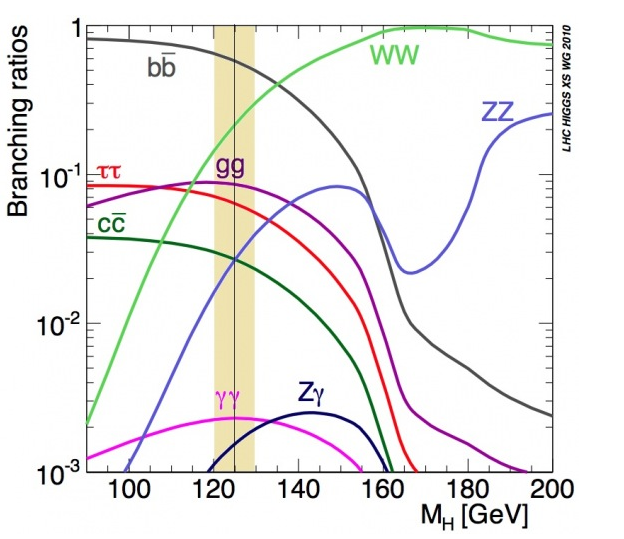
Figure 3: Higgs couplings derived at LHC. Figure from Ref. Dittmaier:2011ti .

III.3 Higgs search at LEP

The clean environment of electron-positron colliders was used first to search for the Higgs boson. At the first stage of LEP, which worked on the Z-pole, the Higgs was searched through the Z decay: $Z\to ff+h$; from the non-observation of such decay it was possible to put the bound: $m_{h}\geq 80$ Gev. Then, the second phase of LEP worked with a cm energy of 200 GeV, and then the search for the Higgs used the reaction (Bjorken mechanism): $e^{+}e^{-}\to Z+h$. Again, the absence of a signal resulted in the bound: $m_{h}\geq 200-m_{Z}\simeq 110$ GeV.

In the late stages of LEP, with a cm energy of about 205 GeV, this bound was slightly extended, up to about 114 GeV. Just when the CERN plans marked that LEP must be closed, in order to start the LHC project, some debate arose because there was a claim for the presence of a Higgs signal with $m_{h}=115$ Gev, which produced lots of enthusiasm among some experimentalist (who pledged for more time and energy for LEP) and also among some theorists, who quickly cooked models that could explain such mass value. The CERN director decided to close LEP and keep the plans for LHC, which a posteriori seems it was the best decision that could be made.

III.4 Higgs production at Hadron colliders

Although at a proton collider it is also possible to produce Higgs bosons with mechanism similar to the one used at LEP, the Bjorken mechanism, namely with quarks and antiquarks colliding to produce the Higgs boson in association with a massive gauge boson ($W$ or $Z$), it turns out that the dominant production mechanism is gluon fusion, despite the fact that it occurs at loop level (with top quarks circulating in the loop). This is so, because gluons carry the largest fraction of momentum from the colliding protons, and also because its parton distribution function provides with the largest luminosities. The production of the Higgs boson with a pair of heavy quarks (top mainly) also reaches a significant cross section. The resulting cross sections for these mechanisms in proton proton colliders, times the branching ratios of some relevant modes, as a function of the cm energy, is shown in fig. 4 Dittmaier:2011ti .

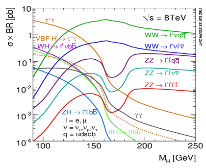
Figure 4: Higgs cross section times BR for different modes, at LHC with Ecm=8 TeV. Figure from Dittmaier:2011ti

III.5 Current Higgs profile from LHC

LHC started collecting data from pp collisions with cm energy of $\sqrt{S}=7$ TeV. After some initial claims for a Higgs signal around 140 GeV, which was again quickly explained by some theory models, the Higgs became real when both collaborations (ATLAS and CMS) announced on July 4th, 2012 that some events on the $\gamma\gamma$ and $ZZ*$ channels were observed, which would correspond to a SM-like Higgs particle with mass $m_{h}=125-126$ GeV. The observation of a resonance decaying into $\gamma\gamma$ indicated that its spin must be either 0 or 2, in accordance with Yang theorem. An scalar, with spin-0, seemed the most natural explanation, which was reinforced by the second decay mode, namely the four-lepton signal, which could be interpreted as coming from the decay $h\to ZZ^{*}\to llll$. Habemus Higgs!

As LHC continued to accumulate luminosity, more Higgs decay modes were observed, which confirmed that the particle observed by ATLAS and CMS was indeed a Higgs-like particle. The interpretation of the Higgs signal was further reinforced after LHC started taking data with higher energy ($\sqrt{S}=13$ TeV). Now the signal can be appreciated even by the public eye, for instance the data from CMS on the four-lepton signal shown in Fig. 5. (from ref. Sirunyan:2017exp ) shows clearly a bump in the invariant mass at 125 GeV (pink) , which stands clearly above the SM backgrounds. There are now a variety of signals that have been measured, which seem all consistent with the SM, as it is shown in figure 6 (left) , from ATLAS (ref. Aad:2015gba ). The mass has been measured with better precision, as it can be seen in figure 6 (right).

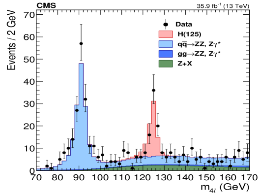
Figure 5: Higgs signal from the decay $h\to ZZ^{*}$ from CMS. Figure from ref. Sirunyan:2017exp

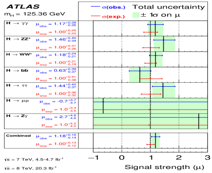
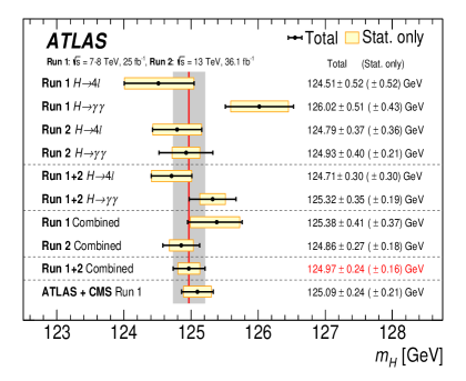
Figure 6: Higgs signals (left) and mass summary (right) from ATLAS. Figure from ref. Aad:2015gba

The current LHC data on Higgs production has been used to derive bounds on deviation from the SM predictions for the Higgs couplings. For instance, figure 7 from Atlas Collaboration (from ref. Aaboud:2018wps ) shows the allowed deviations for the Higgs couplings with gauge bosons and fermions, as parametrized by the constants $\kappa_{V}$ and $\kappa_{F}$. Thus, one can see that best fit lays quite close to the point $\kappa_{V}=\kappa_{F}=1$, which corresponds to the SM limit. However, small deviations are allowed within the precision reached at LHC.

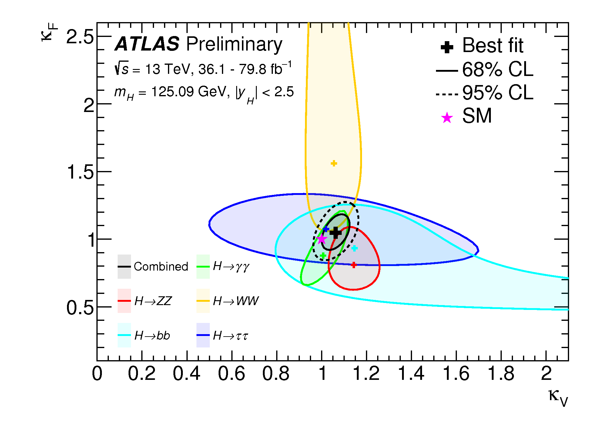
Figure 7: Higgs couplings with vectors and fermions. Figure from ref. Aaboud:2018wps

In essence, the Higgs particle couples to a pair of massive gauge bosons or fermions with a strength proportional to their masses. So far, the LHC has tested only a few of them, namely the Higgs couplings with the gauge bosons and the heaviest fermions of the third family. This is shown in figure 8, from both ATLAS (Aaboud:2018wps ) and CMS (Sirunyan:2018koj ) collaborations, where one can appreciate that the Higgs couplings lay on a straight line, modulo some small deviations for the Higgs coupling with $b\bar{b}$ (which is still consistent at one sigma); the mode $\mu\mu$ has not been detected yet. These results, allow some regions of parameter space for the so-called ”private Higgs” hypothesis, where each fermion type gets its mass from a different Higgs doublet, as it will be discussed briefly in our conclusions. Moreover, these constraints are obtained assuming SM-like pattern for the Higgs couplings, however when one considers new physics, i.e. models beyond the SM Branco:2011iw , it is possible to have non-standard Higgs couplings, including the flavor and CP-violating ones. These will be discussed in the coming sections.

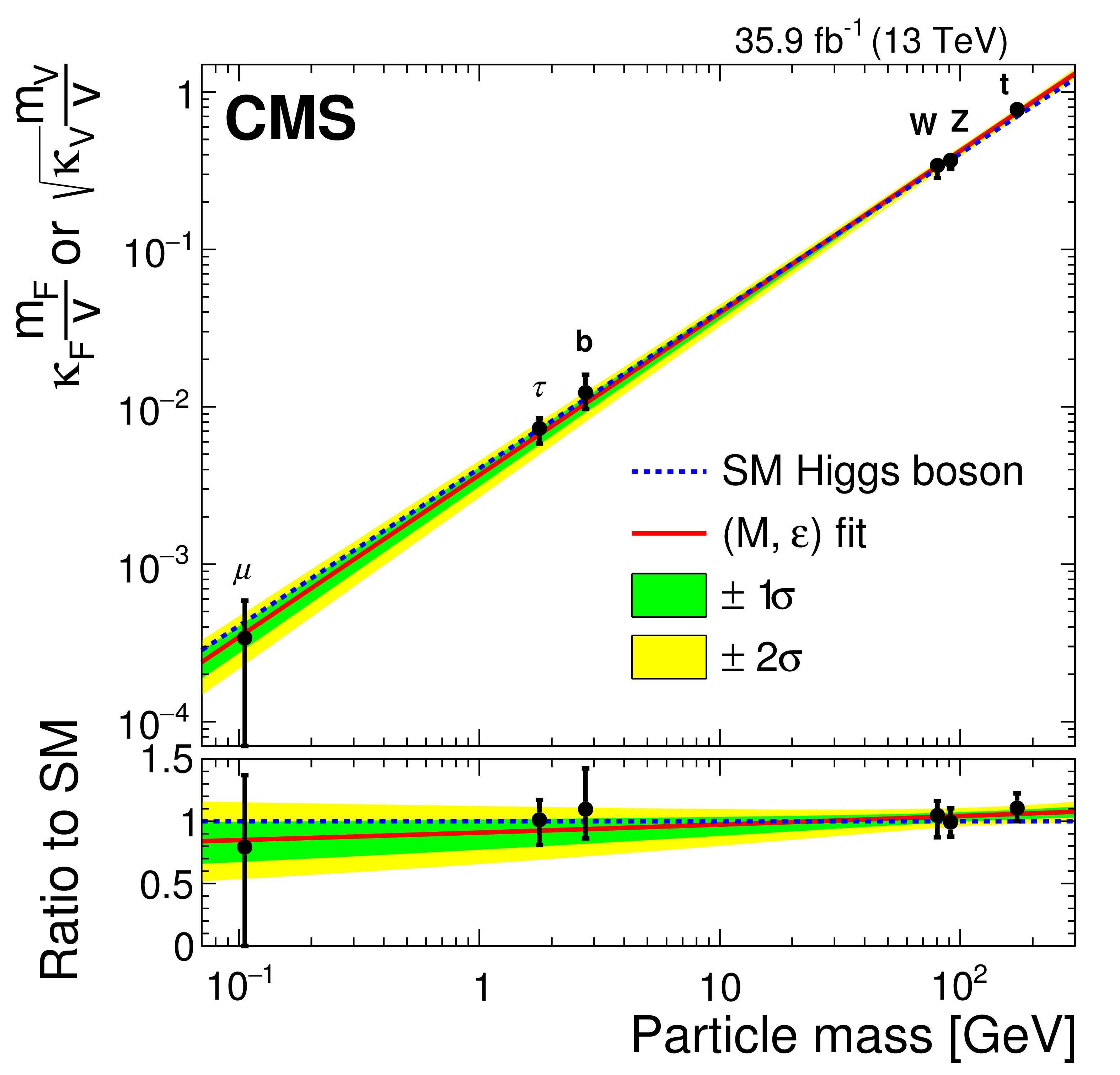
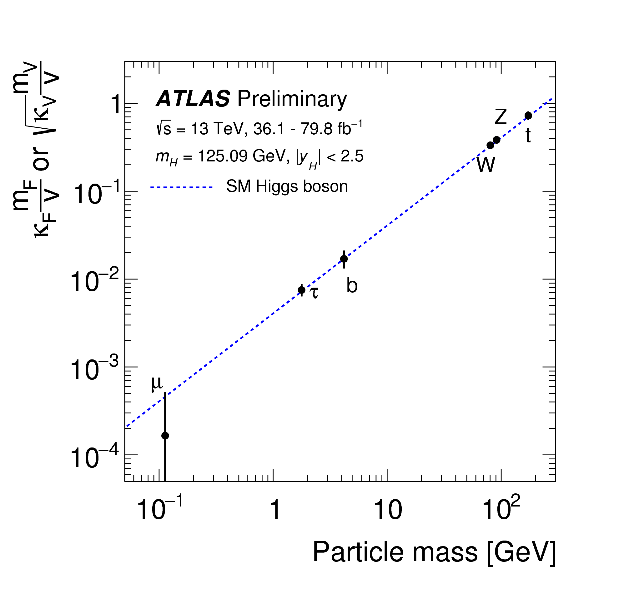
Figure 8: Higgs couplings as function of the mass from CMS (from Sirunyan:2018koj ) and ATLAS (from Aaboud:2018wps ).

IV Beyond the SM Higgs sector: SUSY, flavor and Dark Matter

The SM has several shortcomings that make us suspect that it is not a final theory. For instance, the SM is unable to explain some of the most pressing theoretical problems (unification, flavor, naturalness, etc) Arkani-Hamed:2016kpz , as well as some cosmological data (DM, Dark energy, etc). In particular, finding a possible solution to the hierarchy problem suffered by the SM Higgs boson, has been the driving force behind many of the proposals for extending the SM Pomarol:2012sb .

As we mentioned before, the SM Higgs particle couples to a pair of massive gauge boons or fermions, with an strength proportional to its mass. However, so far LHC provided information on the essential Higgs properties, but this information is based only on a few of the Higgs couplings, i.e. the ones with the heaviest SM fermions and $W,Z$. Then, some questions arise:

• Why is the Higgs mass light? i.e. of the order of the EW scale,

• Do the masses of all fermion types (up-, down-quarks and leptons) arise from a single Higgs doublet? or, are there more Higgs multiplets participating in the game?

• Are the Higgs couplings to fermions diagonal in flavor space?

• Is there any hope to measure the Higgs couplings with the lightest quarks and leptons?

As we shall see next, different answers to these questions arise when one extends the SM. Many of those extensions often include a rich Higgs spectrum, or predict deviations from the SM Higgs properties. These models could either be the realization of elaborated theoretical constructions, or just examples of model building machinery; both of them are usefull at the minimum because they provides a systematic generation of new collider signals to search for, as we shall discuss next. Thus, in order to test these extensions, it will be very important to study the Higgs couplings at LHC and future colliders, and compare with predictions from extended models.

IV.1 Higgs and Supersymmetry

One of the most widely studied extensions of the SM is Supersymmetry. This beautiful idea implies that for each fermions there is a bosonic superpartner, as they are related by a SUSY transformation. The minimal implementation of such idea is the so called minimal SUSY extension of the SM (MSSM) (for a review see Haber:1984rc ; Martin:1997ns ). The MSSM contains 3 families of chiral superfields, which include the quarks and leptons as well as their scalar superpartners, the squarks and sleptons. The gauge sector is described with the vector superfields associated with $SU(3)_{c}\times SU(2)_{L}\times U(1)_{Y}$, and includes the usual gauge bosons, but also their fermionic superpartners, the gauginos. In order to give masses to both up- and down-type fermions, one must have two Higgs doublets, described by chiral superfields, and thus one also has the Higgsinos, as the fermionic superpartners. A discrete symmetry, $R-$ parity, must be imposed in order to respect lepton and baryon number conservation. This $R$- parity implies that superpertners are produced by pairs, and the lightest superpartner must be stable, which provides the seeds for a dark matter candidate, which was considered a great virtue of SUSY models. As the experimental evidence shows, SUSY must be broken, and a realistic scheme is provided by the Soft-breaking terms. Namely, SUSY is assumed to be broken in a Hidden sector, which is then transmitted to the MSSM superpartners by a suitable mediator, which may involve gravity or gauge interactions, or anomaly mediation.

The search for the signals of the superparners has been one of the central goals of current and future colliders Kane:2006hd . However, the LHC has provided bounds on the new physics scale ($\Lambda$), either from the search for new particles or from the effects of new interactions, with values that are now entering into the multi-TeV range. This result is casting some doubts about the theoretical motivations for new physics scenarios that were promoted assuming a mass scale of order TeV. This is particularly disturbing for the concept of naturalness, and its supersymmetric implementation, since the bounds on the mass of superpartners are passing the TeV limit too Kane:2006hd . However, SUSY is such a beautiful theory that it certainly desserves further work on its foundations and possible realization in nature. Thus, one has to wait for the next LHC stages, with higher energy and luminosity, in order to obtain stronger limits, both on the search for new particles, such as heavier Higgs bosons Arganda:2013ve ; Arganda:2012qp ; Chakraborty:2013si or others, and for precision tests of the SM properties.

IV.2 Higgs and flavor: A more flavored Higgs sector

Although the Higgs boson has diagonal couplings to the SM fermions at tree-level, it could mix with new particles that have a non-aligned flavor structure, and this permits to induce corrections to the diagonal Yukawa couplings and/or new flavor-violating (FV) Higgs interactions. Non-standard Higgs couplings are predicted in many models of physics beyond the SM. This could happen, for instance, in extensions of the SM that contain additional scalar fields, which have non-aligned couplings to the SM fermions. When these fields mix with the Higgs boson, it is possible to induce new FV Higgs interactions. This transmission of the flavor structure to the Higgs bosons, was discussed in our earlier work DiazCruz:2002er , where we called it more flavored Higgs boson.

This occurs, for instance, in Froggatt-Nielsen type models, where one includes a SM singlet (Flavon) that participates in the generation of the Yukawa hierarchies. This singlet mixes with the Higgs doublets, and induces FV Higgs couplings at tree-level. The phenomenology for the mixing of the SM Higgs doublet with a flavon singlet has been studied in ref. Dorsner:2002wi ; Arroyo-Urena:2018mvl . Mixing of SM fermions with exotic ones, could also induce FV Higgs couplings at tree-level Langacker:1988ur . On the other hand, within supersymmetric models, like the MSSM, the sfermion/gauginos can have non-diagonal couplings to Higgs bosons and SM fermions. Then, FV couplings of the Higgs with SM fermions could be induced at loop-level DiazCruz:2002er .

In the next section, we shall discuss what is probably the simplest model that contains a more flavored Higgs sector, namely the general two-Higgs doublet model Branco:2011iw .

IV.3 Higgs and Dark Matter

Understanding the nature of dark matter is another aspect of physics beyond the SM, which motivates extensions of the SM. The dark matter could interact with ordinary mater through the Higgs boson, an scenario called the Higgs portal. It could also happen that dark matter is contained within an extension of the Higgs sector, which could include a singlet , an extra (Inert) Higgs doublet, a mixture of them or even a higher-dimensional multiplet Ma:2014rua . DM candidates can also arise in composite Higgs models DiazCruz:2007be .

The case when DM candidate is contained in an extra Higgs doublet is known as the IDM Barbieri:2006dq , which has been studied extensively in the literature Ma:2006km ; LopezHonorez:2006gr ; Krawczyk:2013jta . Including dark matter candidate with extra sources of CP violation, has motivated the constructions of models with inert doublet and singlet Bonilla:2014xba .

Within those models, one can accommodate a neutral and stable scalar particle, which has the right mass and couplings to satisfy the constraints from DM relic density and direct/indirect searches. It also implies modifications of the SM-like Higgs couplings, which must mass the LHC Higgs constraints. The heavy Higgs spectrum provides additional signatures of these models, which could also be searched at future colliders.

V The general 2HDM with Textures and its limits

One of the simplest proposals for physics Beyond the Standard Model, is the so called Two-Higgs Doublet Model (2HDM), which was initially studied in connection with the search for the origin of CP violation Deshpande:1977rw , and later on it was found to be connected with other theoretical ideas in particle physics, such as supersymmetry, extra dimensions Quiros:2006my and strongly interacting systems Pomarol:2012sb ; Aranda:2007tg . Models with extra Higgs doublets are safe regarding the $\rho$ parameter, as they respect the custodial symmetry which protect the relation $\rho=1$.

Several possible realizations of the general 2HDM have been considered in the literature, which have been known as Type I, II and III. The table 1 shows the Higgs assignments that participate in the generation of the masses for the different types of fermions for the 2HDM’s. Model I can have an exact discrete symmetry $Z_{2}$, which permits a possible dark matter candidate coming from the $Z_{2}-$odd scalar doublet Ginzburg:2010wa ; within this type I models, a single Higgs doublet gives mass to the up, down quarks and leptons. The type II model Ginzburg:2004vp assigns one doublet to each fermion type, $\Phi_{1}$ for leptons and down-type quarks, and $\Phi_{2}$ for up-type quarks; this type II model also arises in the minimal SUSY extension of the SM Gunion:1988yc . Both models of type I and II, posses the property of natural flavor conservation, as they respect the Glashow-Weinberg Theorem Glashow:1976nt , which suffices to avoid Flavor Changing Neutral Currents (FCNC) mediated by the Higgs bosons, at the tree-level.

Model type	Up quarks	Down quarks	Charged leptons
2HDM-I	$\Phi_{1}$	$\Phi_{1}$	$\Phi_{1}$
2HDM-II	$\Phi_{2}$	$\Phi_{1}$	$\Phi_{1}$
2HDM-X	$\Phi_{2}$	$\Phi_{2}$	$\Phi_{1}$
2HDM-Y	$\Phi_{2}$	$\Phi_{1}$	$\Phi_{2}$
2HDM-III	$\Phi_{1,2}$	$\Phi_{1,2}$	$\Phi_{1,2}$

Table 1: Higgs interaction with fermions for the different 2HDM types.

There are also other models discussed in the literature called type-X (also called lepton specific) and type-Y (also called flipped) . Although they can be consider as variations of model II, it is important to mention both of them, for completeness and also because they have interesting phenomenology. The Higgs assignments are also shown in table 1.

On the other hand, within the most general version of the 2HDM, where both Higgs doublets could couple to all types of fermions, diagonalization of the full mass matrix, does not imply that each Yukawa matrix is diagonalized, therefore FCNC can appear at tree level Glashow:1976nt . In order to reproduce the fermion masses and mixing angles, with acceptable levels of FCNC Fritzsch:1995nx ; Branco:1999nb ; Hall:1993ca , one can assume that the Yukawa matrices have a certain texture form, i.e. with zeros in different elements, and some possible choices will be discussed in the coming sections.

The general model has been previously referred to as the 2HDM of type III, although this has also been used to denote a different type of model Altmannshofer:2012ar . There are also other relevant sub-cases of the general 2HDM, such as the so-called Minimal Flavor violating 2HDM Buras:2010mh ; D'Ambrosio:2002ex ; Aranda:2012bv . The Aligned model is another example of viable 2HDM Pich:2009sp . Thus, in order to single out the two-Higgs doublet model with textures among this diversity, we proposed to baptize it as the 2HDM-Tx Arroyo:2013tna .

V.1 Yukawa textures: parallel and complementary

The initial construction of the 2HDM with textures Cheng:1987rs , considered first the specific form with six-zeros, and some variations with cyclic textures. In that case a specific pattern of FCNC Higgs-fermion couplings of size $\frac{\sqrt{m_{i}m_{j}}}{v}$ was found, which is known nowadays as the Cheng-Sher ansatz. For this type of Higgs-fermion vertex it is possible to satisfy the FCNC bounds with Higgs masses lighter than O(TeV). The extension of the 2HDM-Tx with a four-zero texture was presented in Zhou:2003kd ; DiazCruz:2004tr . The phenomenological consequences of these textures for Higgs physics (Hermitian 4-textures or non-hermitian 6-textures) were considered in DiazCruz:2004pj , while further phenomenological studies were presented in Wu:2004kr ; Li:2005rr ; Carcamo:2006dp ; DiazCruz:2010yq .

When the fermions ($f=U,D,L$) couples to both Higgs doublets, after SSB the mass matrix is given by:

$$M_{f}=\frac{v_{1}}{\sqrt{2}}Y^{f}_{1}+\frac{v_{2}}{\sqrt{2}}Y^{f}_{2}$$ (26)

Although the texture pattern is defined by considering the zeroes appearing in the fermion mass matrix $M_{f}$, we can have several options for the textures of the Yukawa matrices, $Y_{1}$ an $Y_{2}$. In our work on the 2HDM-Tx Arroyo:2013tna , we considered several possibilities, namely:

• Parallel textures: In this case, we have that both $Y_{1}$ an $Y_{2}$ have the same texture pattern. For instance, if $M_{f}$ is of the four-texture type, then both $Y_{1}$ an $Y_{2}$ have the same four-texture.

• Complementary textures: In this case, we have that both $Y_{1}$ an $Y_{2}$ have different texture pattern, without having elements in common, but in such a way that they produce $M_{f}$ of the given texture type.

• Semi-Parallel textures: In this case, $Y_{1}$ an $Y_{2}$ have different texture patterns, but they have elements in common, and in such a way that they produce $M_{f}$ with a given texture type.

For instance, a four-zero texture mass matrix is of the form:

$${M_{f}}=\left(\begin{array}[]{ccc}0&D&0\\ D^{*}&C&B\\ 0&B^{*}&A\end{array}\right),$$ (30)

In the parallel case we have that both Yukawa matrices ($Y_{i},\,i=1,2$) have the same form, namely:

$$Y_{i}=\begin{pmatrix}0&d_{i}&0\\ d^{*}_{i}&c_{i}&b_{i}\\ 0&b^{*}_{i}&a_{i}\\ \end{pmatrix},$$ (31)

An example of complementary case, where $Y^{f}_{1}$ and ${Y}^{f}_{2}$ (which only has a non-zero 33 entry) combine to produce a mass matrix with four-zero texture, is the following:

$$Y_{1}=\begin{pmatrix}0&d_{1}&0\\ d^{*}_{1}&c_{1}&b_{1}\\ 0&b^{*}_{1}&0\\ \end{pmatrix},\hskip 14.22636ptY_{2}=\begin{pmatrix}0&0&0\\ 0&0&0\\ 0&0&a_{2}\\ \end{pmatrix}.$$ (32)

Finally, an example of semi-parallel textures is the following:

$$Y_{1}=\begin{pmatrix}0&d_{1}&0\\ d^{*}_{1}&c_{1}&b_{1}\\ 0&b^{*}_{1}&a_{1}\\ \end{pmatrix},\hskip 14.22636ptY_{2}=\begin{pmatrix}0&0&0\\ 0&0&0\\ 0&0&a_{2}\\ \end{pmatrix},$$ (33)

in this example, $Y^{f}_{1}$ has a four-zero texture, while ${Y}^{f}_{2}$ has only a non-zero 33 entry.

The detailed study of these Yukawa matrices, including its diagonalization, and the phenomenological consequences, was presented in our ref. Arroyo:2013tna . Next, we shall derive the Yukawa lagrangian of the general 2HDM-III, and we shall employ those textures when considering the 2HDM-Tx.

V.2 The Yukawa lagrangian

Within the general Two-Higgs doublet model, each Higgs doublet couples to a given fermion of type $f$ through the Yukawa matrices $Y^{f}_{1}$ and $Y^{f}_{2}$, which combine after SSB to produce a fermion mass matrix with some texture. We shall write the Yukawa Lagrangian in the 2HDM-III for the quark sector, following the notation from DiazCruz:2004pj , namely:

$$L=Y^{u}_{1}{\bar{Q}}^{0}_{L}{\tilde{\Phi}_{2}}u_{R}^{0}+{{{{Y^{u}_{2}}}}}\bar{Q}_{L}^{0}{\tilde{\Phi}_{2}}u_{R}^{0}+{{{{Y^{d}_{1}}}}}\bar{Q}_{L}^{0}{\Phi_{1}}d_{R}^{0}+{Y^{d}_{2}}\bar{Q}_{L}^{0}{\Phi_{2}}d_{R}^{0}+h.c.$$ (34)

where the quark doublets, quark singlets and Higgs doublets are written as:

$$Q_{L}^{0} = \left(\begin{matrix}u_{L}\\[5.69054pt] d_{L}\\ \end{matrix}\right),\hskip 8.53581pt\overline{Q}_{L}^{0}=\left(\overline{u}_{L},\overline{d}_{L}\right),$$

$${\Phi_{1}} = \left(\begin{matrix}\phi_{1}^{+}\\[5.69054pt] \phi_{1}^{0}\\ \end{matrix}\right),\hskip 8.53581pt{\Phi_{2}}=\left(\begin{matrix}\phi_{2}^{+}\\[5.69054pt] \phi_{2}^{0}\\ \end{matrix}\right),\hskip 8.53581pt$$ (35)

And similarly for the leptons. We have defined the conjugate doublets as: $\tilde{\Phi}_{j}=i\sigma_{2}{\Phi}^{*}_{j}=({\phi_{j}^{0}}^{*},-\phi_{j}^{-})^{T}$, with $\phi_{j}^{0}=(\varphi_{i}+i\chi_{i})/{\sqrt{2}}$.

On the other hand, the CP-properties of the Higgs spectrum depend on the parameters of the Higgs potential. For the 2HDM, this has been studied extensively Accomando:2006ga , using either explicit constructions Ginzburg:2004vp , or employing the basis-independent conditions that classify whether the vacuum respects CP, it violates explicitly CP or CP is spontaneously broken Davidson:2005cw ; Gunion:2005ja ; Maniatis:2007vn ; Ferreira:2010jy . Here we shall follow the methods and notation from ref. Haber:2010bw . Thus, the Higgs mass eigenstates ($H_{i}$) are obtained by the orthogonal rotations, as follows:

$$\left(\begin{array}[]{c}\varphi_{1}\\ \varphi_{2}\\ \chi_{1}\\ \chi_{2}\end{array}\right)=R\left(\begin{array}[]{c}H_{1}\\ H_{2}\\ H_{3}\\ H_{4}\end{array}\right).$$ (36)

We identify $H_{4}=G^{0}$ as the neutral pseudo-Goldstone boson.

For the case with a CP-conserving Higgs potential, one has that $H_{4}=\cos\beta\chi_{1}+\sin\beta\chi_{2}$ is the Goldstone boson, where $\tan\beta=v_{2}/v_{1}$. In this case the couplings of the CP-even Higgs bosons, $h$ and $H$, with $WW$ or $ZZ$ bosons are given by $g_{hVV}=\sin(\beta-\alpha)g^{sm}_{hVV}$ and $g_{HVV}=\cos(\beta-\alpha)g^{sm}_{hVV}$, respectively.

The matrix $R$ can be used to express the Higgs doublets in terms of the physical Higgs mass eigenstate, as follows:

$$\Phi_{1}=\left(\begin{array}[]{c}G^{+}\cos\beta-H^{+}e^{i\xi}\sin\beta\\ \frac{v}{\sqrt{2}}\cos\beta+\frac{1}{\sqrt{2}}\sum_{r=1}^{4}\left(q_{r1}\cos\beta+q_{r2}e^{-i(\theta_{23}+\xi)}\sin\beta\right)H_{r}\end{array}\right),$$ (37)

and

$$\Phi_{2}=\left(\begin{array}[]{c}G^{+}e^{i\xi}\sin\beta+H^{+}\cos\beta\\ \frac{v}{\sqrt{2}}e^{i\xi}\sin\beta+\frac{1}{\sqrt{2}}\sum_{r=1}^{4}\left(q_{r1}e^{i\xi}\sin\beta+q_{r2}e^{-i\theta_{23}}\cos\beta\right)H_{r}\end{array}\right),$$ (38)

The values of $q_{ra}$ are shown in table 2, they are written as combination of the $\theta_{ij}$, which are the mixing angles appearing in the rotation matrix that diagonalize the mass matrix for neutral Higgs.

$r$	$q_{r1}$	$q_{r2}$
1	$\cos\theta_{12}\cos\theta_{13}$	$-\sin\theta_{12}-i\cos\theta{12}\sin\theta_{13}$
2	$\sin\theta_{12}\cos\theta_{13}$	$\cos\theta_{12}-i\sin\theta{12}\sin\theta_{13}$
3	$\sin\theta_{13}$	$i\cos\theta_{13}$
4	$i$	0

Table 2: Mixing angles for Higgs bosons which consider spontaneous and explicit CPV.

After substituting these expressions in the Yukawa Lagrangian one obtains the Higgs-fermion interactions for the general 2HDM-III. They are written in terms of the quark mass matrices ($q=U,D$), which receive contributions from both vev’s, namely: $M_{q}=\frac{v_{1}}{\sqrt{2}}Y^{q}_{1}+\frac{v_{2}}{\sqrt{2}}Y^{q}_{2}$. As we mentioned in the previous sub-section, the diagonal form of the quark mass matrices ($\bar{M}_{q}$) is obtained by applying the bi-unitary transformations, namely: $\bar{M}_{q}=V^{q}_{L}M_{q}V^{q\dagger}_{R}$. Explicit expressions for these matrices are shown in Arroyo:2013tna . Thus, the couplings of the neutral Higgs boson ($H_{r}$, $a=1,2,3$) with fermions of type f can be expressed in the form of Eq. 23, as follows:

$${\cal{L}}_{f}=H^{a}\bar{f}_{i}(S^{fr}_{ij}+i\gamma_{5}P^{fr}_{ij})f_{j}$$ (39)

For the up-type quarks, the factors $S_{ij}^{ur}$ and $P_{ij}^{ur}$ are written as:

$$S_{ijr}^{ur} = \frac{1}{2v}\bar{M}_{ij}^{U}\left(q_{k1}^{\ast}+q_{k1}-\tan\beta\left(q_{k2}^{\ast}e^{i\left(\theta_{23}+\xi\right)}+q_{k2}e^{-i\left(\theta_{23}+\xi\right)}\right)\right)$$ (40)

$$+\frac{1}{2\sqrt{2}\cos\beta}\left(q_{k2}^{\ast}e^{i\theta_{23}}\widetilde{Y}_{2ij}^{U}+q_{k2}e^{-i\theta_{23}}\widetilde{Y}_{2ij}^{U\dagger}\right)$$

and

$$P_{ij}^{ur} = \frac{1}{2v}\bar{M}_{ij}^{U}\left(q_{k1}^{\ast}-q_{k1}-\tan\beta\left(q_{k2}^{\ast}e^{i\left(\theta_{23}+\xi\right)}-q_{k2}e^{-i\left(\theta_{23}+\xi\right)}\right)\right)$$ (41)

$$+\frac{1}{2\sqrt{2}\cos\beta}\left(q_{k2}^{\ast}e^{i\theta_{23}}\widetilde{Y}_{2ij}^{U}-q_{k2}e^{-i\theta_{23}}\widetilde{Y}_{2ij}^{U\dagger}\right).$$

Similarly, for the down-type quarks we find:

$$S_{ij}^{dr} = \frac{1}{2v}\bar{M}_{ij}^{D}\left[q_{k1}+q_{k1}^{\ast}-\tan\beta\left(q_{k2}^{\ast}e^{i\left(\theta_{23}+\xi\right)}+q_{k2}e^{-i\left(\theta_{23}+\xi\right)}\right)\right]$$ (42)

$$+\frac{1}{2\sqrt{2}\cos\beta}\left(q_{k2}e^{-i\theta_{23}}Y_{2}^{D}+q_{k2}^{\ast}e^{i\theta_{23}}\widetilde{Y}_{2}^{D\dagger}\right)$$

and

$$P_{ij}^{dr} = \frac{1}{2v}\bar{M}_{ij}^{D}\left[q_{k1}-q_{k1}^{\ast}+\tan\beta\left(q_{k2}^{\ast}e^{i\left(\theta_{23}+\xi\right)}-q_{k2}e^{-i\left(\theta_{23}+\xi\right)}\right)\right]$$ (43)

$$+\frac{1}{2\sqrt{2}\cos\beta}\left(q_{k2}e^{-i\theta_{23}}\widetilde{Y}_{2}^{D}-q_{k2}^{\ast}e^{i\theta_{23}}\widetilde{Y}_{2}^{D\dagger}\right).$$

This Lagrangian is the most general one, which includes the possibility to have i) Deviations from the SM (diagonal) Higgs couplings ii) New flavor violating Higgs couplings and iii) New sources of CP violation, coming either from the Higgs potential or the Yukawa matrices. Further simplifications can be obtained when one assumes that the Yukawa matrices are hermitic, i.e. $\widetilde{Y}_{2}^{Q}=\widetilde{Y}_{2}^{Q\dagger}$ (with $Q=U,D$) or when the Higgs potential is CP conserving.

Next we shall present some limiting cases for the couplings of Higgs $H^{r}$ ($r=1,2,3$) with fermions of type f , expressed in terms of the factors $S^{fa}_{ij}$, $P^{fa}_{ij}$, which in turn can be written as:

$$S^{fr}_{ij} = \frac{gm_{i}}{2m_{W}}c_{fr}\delta_{ij}+\frac{g}{2}d_{fr}\eta^{f}_{ij}$$ (44)

$$P^{fr}_{ij} = \frac{gm_{i}}{2m_{W}}e_{fr}\delta_{ij}+\frac{g}{2}g_{fr}\eta^{{}^{\prime}f}_{ij}$$ (45)

As it is discussed in detail in ref. DiazCruz:2004tr , when one assumes parallel Yukawa matrices of the four-textur type, one can express those factors in terms of the quark masses, the mixing angles and some flavor-dependent parameters. In fact, in that case the $\eta^{f}_{ij}$ parameters satisfy the Cheng-Sher ansazt and are universal (the same for all Higgs bosons), then it is possible, and convenient, to express them as follows:

$$\eta^{f}_{ij}=\tilde{\chi}^{f}_{ij}\frac{\sqrt{m_{i}m_{j}}}{m_{W}}$$ (46)

The parameters $\tilde{\chi}^{f}_{ij}$ can be constrained by considering all types of low energy FCNC transitions, which produce the viable regions of parameter space.

V.3 The 2HDM-III with non-Hermitian Yukawa matrices and CPC Higgs potential

In this case we shall consider that the Higgs sector is CP conserving (CPC), while the Yukawa matrices are non-hermitian. Then, without loss of generality, we can assume that $H_{3}=A$ is CP odd, with $H_{1}=h$ and $H_{2}=H$ are CP even, then: $\cos\theta_{12}=\sin\left(\beta-\alpha\right)$, $\sin\theta_{12}=\cos\left(\beta-\alpha\right)$, $\sin\theta_{13}=0$, and $e^{-i\theta_{13}}=1$. The expressions for the neutral Higgs masses eigenstates can be written now in terms of the angles $\alpha$ (which diagonalizes the CP-even Higgs bosons) and $\beta$ ($\tan\beta=v_{2}/v_{1}$):

$$\Phi_{a}^{0} = \frac{1}{\sqrt{2}}\left(v+h^{0}\sin\left(\beta-\alpha\right)+H^{0}\cos\left(\beta-\alpha\right)+iG^{0}\right)\widehat{v}_{a}$$ (47)

$$+\frac{1}{\sqrt{2}}\left(h^{0}\cos\left(\beta-\alpha\right)-H^{0}\sin\left(\beta-\alpha\right)+iA^{0}\right)\widehat{w}_{a},$$

where $a=1,2$, and for the CP-conserving limit $\widehat{v}_{a}$ and $\widehat{w}_{a}$ have a vanishing phase $\xi=0$. Here, the components of $\hat{v}_{a}$, $\hat{w}_{a}$ are given as:

$$\widehat{v}=\left(\begin{array}[]{cc}\hat{v}_{1},&\hat{v}_{2}\end{array}\right)=\left(\begin{array}[]{cc}\cos\beta,&e^{i\xi}\sin\beta\end{array}\right)$$ (48)

and

$$\widehat{w}=\left(\begin{array}[]{cc}\hat{w}_{1},&\hat{w}_{2}\end{array}\right)=\left(\begin{array}[]{cc}-e^{-i\xi}\sin\beta,&\cos\beta\end{array}\right).$$ (49)

Additionally, when one assumes a 4-texture for the Yukawa matrices, the Higgs-fermion couplings further simplify as $\widetilde{Y}_{2ij}^{U}=\chi_{ij}\frac{\sqrt{m_{i}m_{j}}}{v}$ . Then, coefficient (40) and (41) for up sector for $r=1,2,3$, and with $H_{1}=h$ being identified as the light SM-like Higgs boson, are shown in table III.

Coefficient	$c_{ui}$	$d_{ui}$	$e_{ui}$	$g_{ui}$
$H_{1}$	$\sin(\beta-\alpha)-\tan\beta\cos(\beta-\alpha)$	$\frac{\cos(\beta-\alpha)}{\cos\beta}$	0	$\frac{\cos(\beta-\alpha)}{\cos\beta}$
$H_{2}$	$\cos(\beta-\alpha)-\tan\beta\sin(\beta-\alpha)$	$\frac{\sin(\beta-\alpha)}{\cos\beta}$	0	$\frac{\sin(\beta-\alpha)}{\cos\beta}$
$H_{3}$	0	$\frac{1}{\cos\beta}$	$\tan\beta$	$\frac{1}{\cos\beta}$

Table 3: Coefficients for Higgs-Fermion couplings.

The $\eta$ parameters are given as follows:

$$\eta^{u}_{ij}=\frac{\sqrt{m_{i}m_{j}}}{2\sqrt{2}v}\left(\chi_{ij}+\chi_{ij}^{{\dagger}}\right)$$ (50)

$$\eta^{u^{\prime}}_{ij}=\frac{\sqrt{m_{i}m_{j}}}{2\sqrt{2}v}\left(\chi_{ij}-\chi^{{\dagger}}_{ij}\right)$$ (51)

Similar expressions are obtained for d-type quarks and leptons.

V.4 The 2HDM-III with Hermitian Yukawa matrices and CPV Higgs

In this case we assume the hermiticity condition for the Yukawa matrices, but the Higgs sector could be CP violating. For simplicity we shall consider that the Hermitic Yukawa matrices that obey a four-texture form, but now CP is violated in the Higgs sector.

Then, one obtains the following expressions for the couplings of the neutral Higgs bosons with the up-type quarks, namely:

$$S_{ijr}^{u}=\frac{1}{2v}M_{ij}^{U}\left[q_{r1}^{\ast}+q_{r1}-\tan\beta\left(q_{r2}^{\ast}+q_{r2}\right)\right]+\frac{\sqrt{m_{i}m_{j}}}{2\sqrt{2}v\cos\beta}\chi_{ij}\left(q_{r2}^{\ast}+q_{r2}\right)$$ (52)

and

$$P_{ijr}^{u}=\frac{1}{2v}M_{ij}^{U}\left[q_{r1}^{\ast}-q_{r1}-\tan\beta\left(q_{r2}^{\ast}-q_{r2}\right)\right]+\frac{\sqrt{m_{i}m_{j}}}{2\sqrt{2}v\cos\beta}\chi_{ij}\left(q_{r2}^{\ast}-q_{r2}\right)$$ (53)

similar expressions can be obtained for the down-type quarks and leptons, as well as for the charged Higgs couplings.

V.5 The 2HDM-III with Hermitic textures and CP-conservation (2HDM-Tx)

In this case we assume the hermiticity condition for the Yukawa matrices, and the Higgs sector is CP conserving. For simplicity we shall consider that the Yukawa matrices obey a four-texture form. Then, the Higgs-fermion couplings take the following form. For $r=1,2$ one gets,

$$S_{ij1}^{u} = \frac{1}{v}M_{ij}^{U}\left(\sin(\beta-\alpha)+\tan\beta\cos(\beta-\alpha)\right)$$ (54)

$$-\frac{\chi_{ij}\sqrt{m_{i}m_{j}}}{\sqrt{2}v}\frac{\cos(\beta-\alpha)}{\cos\beta},$$

$$S_{ij2}^{u}=-\frac{1}{v}M_{ij}^{U}\frac{\sin\alpha}{\cos\beta}+\frac{\chi_{ij}\sqrt{m_{i}m_{j}}}{\sqrt{2}v}\frac{\sin(\beta-\alpha)}{\cos\beta},$$ (55)

For both Higgs bosons $H_{1}$ and $H_{2}$ one has: $P_{ij1}^{u}=P_{ij2}^{u}=0$ On the other hand, for $r=3$, one has $S_{ij3}^{u}=0$ and:

$$P_{ij3}^{u}=-i\frac{\chi_{ij}\sqrt{m_{i}m_{j}}}{\sqrt{2}v\cos\beta}.$$ (56)

V.6 The 2HDM of type I, II, X, Y: CPC case

In all these cases each fermion type (U,D,L) couple only with one Higgs doublet, as shown in table I. Now, we have that: $d_{fr}=g_{fr}=0$, while the non-zero coupling constants ($c_{f}$ for $h,H$ or $e_{f}$ for $A$), are shown in table IV for models I and II, while table V shows the corresponding couplings for models X and Y.

Higgs boson	$c_{u}$	$c_{d}$	$c_{l}$
$h$ (I)	$\cos\alpha/\sin\beta$	$\cos\alpha/\sin\beta$	$\cos\alpha/\sin\beta$
$h$ (II)	$\cos\alpha/\sin\beta$	-$\sin\alpha/\cos\beta$	-$\sin\alpha/\cos\beta$
$H$ (I)	$\sin\alpha/\sin\beta$	$\sin\alpha/\sin\beta$	$\sin\alpha/\sin\beta$
$H$ (II)	$\sin\alpha/\sin\beta$	$\cos\alpha/\cos\beta$	$\cos\alpha/\cos\beta$
$A$ (I)	$\cot\beta$	-$\cot\beta$	-$\cot\beta$.
$A$ (II)	$\cot\beta$	$\tan\beta$	$\tan\beta$.

Table 4: Higgs interaction with fermions for flavor conserving 2HDM of types I and II.

Higgs boson	$c_{u}$	$c_{d}$	$c_{l}$
$h$ (X)	$\cos\alpha/\sin\beta$	$\cos\alpha/\sin\beta$	-$\sin\alpha/\cos\beta$
$h$ (Y)	$\cos\alpha/\sin\beta$	-$\sin\alpha/\cos\beta$	$\cos\alpha/\sin\beta$
$H$ (X)	$\sin\alpha/\sin\beta$	$\sin\alpha/\sin\beta$	$\cos\alpha/\cos\beta$
$H$ (Y)	$\sin\alpha/\sin\beta$	$\cos\alpha/\cos\beta$	$\sin\alpha/\sin\beta$
$A$ (X)	$\cot\beta$	-$\cot\beta$	$\tan\beta$.
$A$ (Y)	$\cot\beta$	$\tan\beta$	-$\cot\beta$.

Table 5: Higgs interaction with fermions for flavor conserving 2HDM of types X and Y.

Then, the Higgs couplings with fermions and gauge bosons in these models are determined by the mixing angles $\alpha$ (which diagonalizes the neutral CP-even Higgs mass matrix) and $\tan\beta=v_{2}/v_{1}$. For a quick test of Higgs couplings, one can rely on the Universal Higgs fit Giardino:2013bma , where bounds on the parameters $\epsilon_{X}$ are derived, they are defined as the (small) deviations of the Higgs couplings from the SM values, i.e. $g_{hXX}=g^{sm}_{hXX}(1+\epsilon_{X})$. We find very convenient, in order to use these results and get a quick estimate of the bounds, to write our parameters as: $\eta_{X}=1+\epsilon_{X}$. For fermions, the allowed values are: $\epsilon_{t}=-0.21\pm 0.23$, $\epsilon_{b}=-0.19\pm 0.3$, $\epsilon_{\tau}=0\pm 0.18$. However, specific tests of the mixing angles $\alpha$ and $\beta$, or combinations of them, have been presented by the LHC collaborations; for instance the CMS constraints on the mixing angles $\alpha$ and $\beta$, for 2HDM-I and 2HDM-II, are shown in Figure 9 CMS:2016qbe .

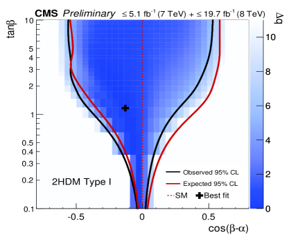
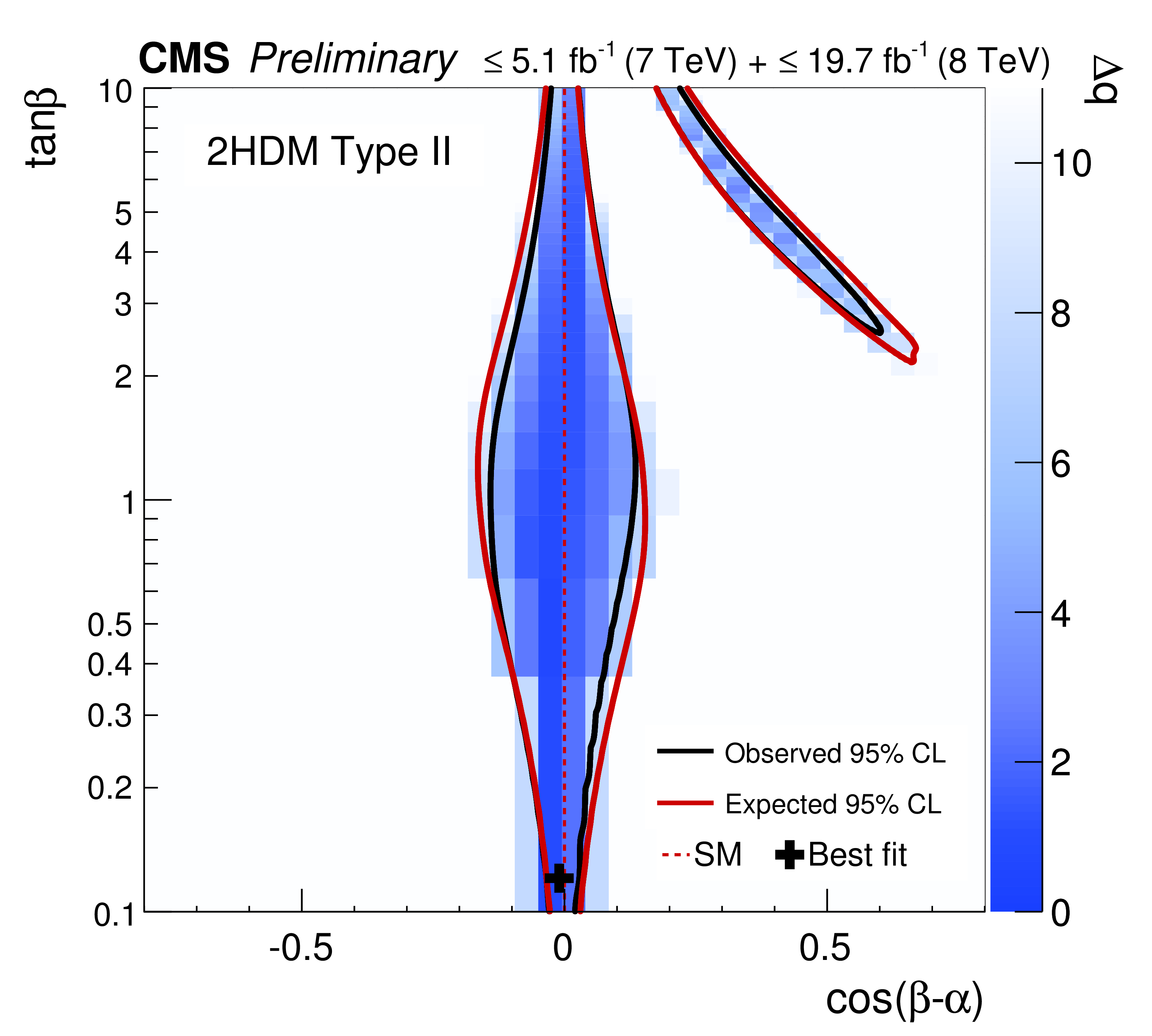
Figure 9: CMS constraints on the mixing angles $\alpha$ and $\beta$, for 2HDM-I and 2HDM-II. Figures from ref. CMS:2016qbe .

On the other hand, the Higgs coupling with the fermions ($b\bar{b},c\bar{c},\tau^{+}\tau^{-}$), which could be measured at next-linear collider (NLC) with a precision of a few percent. This is particularly interesting for the large $\tan\beta$ region, where the corrections to the coupling $h\bar{b}b$ could change the sign Modak:2016cdm , and modify the dominant decay of the light Higgs, as well as the associated production of the Higgs with b-quark pairs Balazs:1998nt ; DiazCruz:1998qc .

VI The flavor violating Higgs and top decays signals

In the models that we are interested in, both flavor and CP-violation could occur, either at tree- or loop-levels. Within the 2HDM-Tx it occurs at tree-level, with large rates that make it feasible to be searched at current and future colliders. In order to evaluate the viability of the Higgs signals, one needs first to consider all low-energy processes, and use the current bounds to look for allowed regions of parameter space. This is shown in figure 10, from Arroyo:2013tna , with some emphasis on the LFV processes. Figure 10-left shows the allowed region in the plane $\tan\beta-\cos(\beta-\alpha)$, after LHC constraints, while figure 10-right shows the bounds from flavor-dependent processes. One of the most sensitive constraint is provided by the muon anomalous magnetic moment, which deviates from the SM, and it is difficult to reproduce with the 2HDM of type I and II, but for model III we do find viable regions of parameter space. For instance, for values around $\tan\beta\simeq 7$, the allowed heavy Higgs mass range is: $500<m_{H}<1000$ GeV; another region around $\tan\beta\simeq 12-15$ is also allowed, but now only for $850<m_{H}<1000$ GeV.

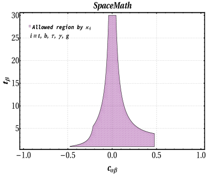
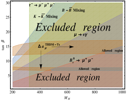
Figure 10: Constraints from flavor physics on 2HDM. Figures from Arroyo:2013tna .

VI.1 LFV Higgs decays

Within the SM, LFV processes vanish at any order of perturbation theory, which motivates the study of SM extensions that predict sizable LFV effects that could be at the reach of detection. In particular, the observation of neutrino oscillations, which is associated with massive neutrinos, motivates the occurrence of Lepton Flavor Violation (LFV) in nature Valle:2018pgs ; Ma:2006fn , which could be tested with the charged lepton decays, $l_{i}\to l_{j}\gamma$ and $l_{i}\to l_{j}\bar{l}_{k}l_{k}$. Another interesting possibility, which became even more relevant after the Higgs discovery, is the decay $h\to\tau\mu$, which was studied first in Refs. Pilaftsis:1992st ; DiazCruz:1999xe , with subsequent analyses on the detectability of the signal appearing soon after Han:2000jz ; Assamagan:2002kf ; Kanemura:2005hr ; McKeen:2012av . This motivated a plethora of calculations in the framework of several SM extensions, such as theories with massive neutrinos, supersymmetric theories, etc. Cotti:2002zq ; Arganda:2004bz ; DiazCruz:2002er ; Brignole:2004ah ; DiazCruz:2008ry ; Curtin:2013fra . (For more on LFV Higgs decays see also Arana-Catania:2013xma ; Arhrib:2012ax ; Harnik:2012pb ; Goudelis:2011un ; GomezBock:2005hc ).

Nowadays, the decay $h\to\tau\mu$ is included in the Higgs boson studies performed at LHC, which offers a great opportunity to search for new physics at the LHC. Along this line, a slight excess of $h\to\tau\mu$ signal was reported at the LHC run I, with a significance of 2.4 standard deviations Khachatryan:2015kon , but subsequent studies Aad:2016blu ; Sirunyan:2017xzt ruled out such an excess and instead put the limit $BR(h\to\bar{\mu}\tau)<1.2\times 10^{-2}$ with 95% C.L. Current bounds on LFV Higgs decays from CMS are shown in figure 11, for the plane of LFV Higgs couplings $|Y_{\tau\mu}|-|Y_{\mu\tau}|$, which also shows the constraints obtained from LFV lepton decays; we can see that the LFV Higgs decay provides the strongest constraints on these parameters.

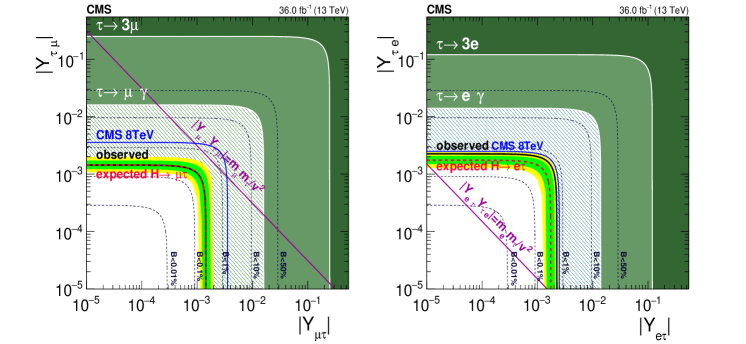
Figure 11: Bounds on LFV Higgs couplings. Figure from Sirunyan:2017xzt .

Now we can use those strongest constraints on the LFV Higgs decay, in order to test the 2HDM-Tx, for the choices of textures that me mentioned before: Parallel, Complementary and semi-Parallel. This is shown in figure 12, for the cases studied in ref. Arroyo:2013tna , and we can see that all of them satisfy the current LHC limits, but the predicted rates could tested at the coming LHC runs..

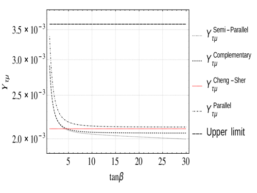
Figure 12: Constraints on LFV Higgs couplings. Figure from Arroyo:2013tna .

VI.2 FCNC top decays

Top quark rare decays has been studied for several years as a channel to search of new physics LDCtopfv ; Eilam:1991 ; Mele:1998 ; Aguilar:2003 ; Jenkins:1996zd ; Lorenzo:1999 , which included a variety of theoretical calculation for $BR(t\rightarrow ch)$ Bar-Shalom:1998 ; DiazCruz:2012xa ; DiazCruz:2001gf . We use the following expression for the branching ratio: $BR(t\rightarrow ch)=\frac{\Gamma(t\rightarrow ch)}{\Gamma_{tot}}$, where the total top width is given by: $\Gamma_{tot}\approx 1.55GeV$, and the width for the FCNC top decay (in the CPC case) is:

$$\Gamma(t\rightarrow ch)\approx\frac{g^{2}_{htc}}{32\pi}\frac{v^{2}}{f^{2}}m_{t}\left(1-\frac{m^{2}_{h}}{m_{t}^{2}}\right)^{2}$$ (57)

The resulting rates for $BR(t\to ch)$, are shown in figure 13, for the cases considered in ref. Arroyo:2013tna .

So far, LHC has provided the limit $B.R.(t\rightarrow ch)<2\times 10^{-3}$ Khachatryan:2014jya . On the other hand, Ref. AguilarSaavedra:2000aj ; topfcnc ; Chen:2013qta , provides some estimates for the branching ratios for $t\rightarrow ch$ that could be proved at the different phases of LHC. For instance, it is claimed there that top decay processes provide the best channel to discover top FCNC interactions, while only in some cases it is surpassed by single top production, when up and charm quark FCNC interactions are involved. In some of the examples discussed in ref. topfcnc , the maximum rates predicted to be observable, with a 3 $\sigma$ statistical significance or more, is about is $BR<5.8\times 10^{-5}$, for one LHC year with a luminosity of 6000 $fb^{-1}$. This implies that the top FCNC branching ratio that arise within the 2HDM-Tx can be proved at LHC.

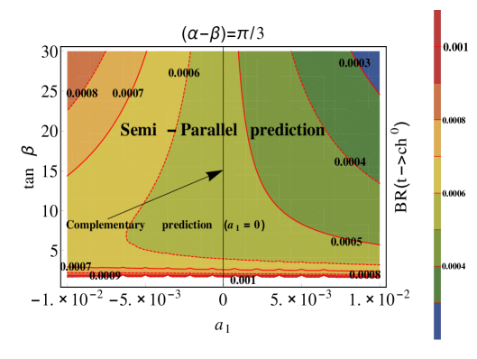
Figure 13: Constraints on Higgs couplings and implications $BR(t\to ch)$. Figure from Arroyo:2013tna .

VII Conclusion and outlook

One of the most important task of future colliders is to study the properties of the Higgs-like particle with $m_{h}=126$ GeV discovered at the LHC. Current measurements of its spin, parity, and interactions, seems consistent with the SM. We have reviewed the essentials of the SM Higgs sector, going from the model definition up to its phenomenology. Then, we presented the motivation for the multi-Higgs models, with particular emphasis on the general 2HDM. Constraints on the Higgs-fermion couplings, derived from Higgs search at LHC, and their implications were discussed too. In the down-quark sector, there are a interesting aspects to study, such as the rates for rare b-decays. Furthermore, as a consequence of Lepton Flavor Violating (LFV) Higgs interactions, the decay $h\to\tau\mu$ can be induced at rates that could be detected at future colliders. The complementarity of future colliders has been studied in Kanemura:2014dea . For the up sector, perhaps the most interesting signal is provided by the FCNC top decay $t\to ch$, which can be studied at LHC.

Within the SM we have only one Higgs doublet giving masses to all type of fermions, and thus its couplings to fermions and gauge bosons are proportional to the particle mass, and they lay on a single line, when plotted as function of the particle mass. But it is desirable to test this property and study models where more than one Higgs multiplet participates in the fermion mass generation. In fact, the THDM is one example where such scheme arises; in this case we have that the fermion couplings lay on two lines, one for up-type quarks and one for leptons and down-type quarks. There are also models where each fermion type gets its mass from a private Higgs, for this we need at least 3 Higgs doublets. In this case, the Higgs couplings as function of the fermion mass lays on three different lines. We have also studied these extended Higgs sector, both for a Non-SUSY model Diaz-Cruz:2014pla and for a SUSY model (4HDM) Diaz-Cruz:2019emo . Besides serving us as an specific model to test the pattern of Higgs couplings, and new physics, this model can also be motivated from the scenarios having one Higgs for each generation, such as the $E_{6}$ GUT model and the superstring-inspired models Aranda:2000zf .

To test this type of models one needs to measure Higgs couplings with fermions of at least two generations. So far, LHC has measured couplings with fermions of the 3rd generation, and there is some chance to measure couplings with charm and muons, which will permit to test the private Higgs hypothesis. At linear colliders it will be possible to measure these couplings with better precision; more recently there have appeared some claims that the coupling with strange quarks is also possible, both the flavor-conserving Duarte-Campderros:2018ouv and flavor-violating ones Barducci:2017ioq . Furthermore, this could also be possible within the models with Higgs portal to dark matter, In such case, the direct detection of DM depends on the Higgs interaction with nucleons, which in turn depends on the Higgs coupling with light quarks. Therefore, by searching for DM-nucleon dispersion one is testing the Higgs coupling with light quarks. Similar remarks hold when one considers $e-\mu$ conversion, where the Higgs nucleon interaction also plays a role.

Thus, nature could be extra benevolent, and by permitting the existence of a light Higgs boson, it could have provided us with a tool to search for physics beyond the SM. The detection of the Higgs boson could be of such relevance, that it may be the key to find what lies beyond the SM, with implications ranging from flavor physics to dark matter, supersymmetry and even cosmology Espinosa:2013lma .

Acknowledgements

I acknowledge support from CONACYT-SNI (Mexico) and VIEP(BUAP). I would like to thank M.A. Perez, G.L. Kane, and A. Mendez, for their support and many lessons on Higgs physics. Special thanks to my classmate C.P. Yuan, and to A. Rosado, G. Lopez-Castro and A. Aranda, for many years of fruitful collaborations. I also learned from my former postdocs and students on the topics that appear in this paper: M. Arroyo, J. Halim, B. Larios, J. Hernandez, Olga Felix, R. Noriega-Papaqui, J. Orduz, U. Saldana. M.Arroyo and B. Larios helped me with some of the figures, and the higgsitos M. Prez de Leon and R. Garcia assisted me by reading the draft and suggested some corrections.

References

- [1] G. Aad et al. [ATLAS Collaboration], Phys. Lett. B 716, 1 (2012) [arXiv:1207.7214 [hep-ex]].
- [2] S. Chatrchyan et al. [CMS Collaboration], Phys. Lett. B 716, 30 (2012) [arXiv:1207.7235 [hep-ex]].
- [3] S. L. Glashow, Nucl. Phys. 22, 579 (1961). doi:10.1016/0029-5582(61)90469-2
- [4] S. Weinberg, Phys. Rev. Lett. 19, 1264 (1967). doi:10.1103/PhysRevLett.19.1264
- [5] A. Salam, Conf. Proc. C 680519, 367 (1968).
- [6] P. W. Higgs, Phys. Rev. Lett. 13, 508 (1964).
- [7] F. Englert and R. Brout, Phys. Rev. Lett. 13, 321 (1964). doi:10.1103/PhysRevLett.13.321
- [8] G. S. Guralnik, C. R. Hagen and T. W. B. Kibble, Phys. Rev. Lett. 13, 585 (1964). doi:10.1103/PhysRevLett.13.585
- [9] S. L. Glashow, J. Iliopoulos and L. Maiani, Phys. Rev. D 2, 1285 (1970). doi:10.1103/PhysRevD.2.1285
- [10] M. J. G. Veltman, Nucl. Phys. B 7, 637 (1968). doi:10.1016/0550-3213(68)90197-1
- [11] J. R. Ellis, M. K. Gaillard and D. V. Nanopoulos, Nucl. Phys. B 106, 292 (1976). doi:10.1016/0550-3213(76)90382-5
- [12] H. M. Georgi, S. L. Glashow, M. E. Machacek and D. V. Nanopoulos, Phys. Rev. Lett. 40, 692 (1978). doi:10.1103/PhysRevLett.40.692
- [13] S. L. Glashow, D. V. Nanopoulos and A. Yildiz, Phys. Rev. D 18, 1724 (1978). doi:10.1103/PhysRevD.18.1724
- [14] M. J. G. Veltman, Phys. Lett. 70B, 253 (1977). doi:10.1016/0370-2693(77)90532-9
- [15] J. F. Gunion, H. E. Haber, G. L. Kane and S. Dawson, Front. Phys. 80, 1 (2000).
- [16] M. Carena and H. E. Haber, Prog. Part. Nucl. Phys. 50, 63 (2003) doi:10.1016/S0146-6410(02)00177-1 [hep-ph/0208209].
- [17] A. Djouadi, Phys. Rept. 457, 1 (2008) doi:10.1016/j.physrep.2007.10.004 [hep-ph/0503172].
- [18] G. Kane, private communication.
- [19] J. Erler, AIP Conf. Proc. 917, 244 (2007) [hep-ph/0701261].
- [20] J. R. Espinosa, C. Grojean, M. Muhlleitner and M. Trott, JHEP 1212, 045 (2012) [arXiv:1207.1717 [hep-ph]].
- [21] K. Cheung, J. S. Lee and P. -Y. Tseng, JHEP 1401, 085 (2014) [arXiv:1310.3937 [hep-ph]].
- [22] J. Ellis, V. Sanz and T. You, arXiv:1404.3667 [hep-ph].
- [23] N. Arkani-Hamed, R. T. D’Agnolo, M. Low and D. Pinner, JHEP 1611, 082 (2016) doi:10.1007/JHEP11(2016)082 [arXiv:1608.01675 [hep-ph]].
- [24] E. Accomando et al., doi:10.5170/CERN-2006-009 hep-ph/0608079.
- [25] G. Altarelli, Phys. Scripta T 158, 014011 (2013) doi:10.1088/0031-8949/2013/T158/014011 [arXiv:1308.0545 [hep-ph]].
- [26] J. Ellis, M. K. Gaillard and D. V. Nanopoulos, doi: arXiv:1504.07217 [hep-ph].
- [27] H. E. Haber, PoS CHARGED 2016, 029 (2017) doi:10.22323/1.286.0029 [arXiv:1701.01922 [hep-ph]].
- [28] S. Dawson, C. Englert and T. Plehn, arXiv:1808.01324 [hep-ph].
- [29] G. Kane, arXiv:1802.05199 [hep-ph].
- [30] J. D. Wells, Stud. Hist. Philos. Mod. Phys. B 62, 36 (2018). doi:10.1016/j.shpsb.2017.05.004
- [31] W. S. Hou, Phys. Lett. B 296, 179 (1992). doi:10.1016/0370-2693(92)90823-M
- [32] T. Lancaster and S. J. Blundell, “Quantum Field Theory for the Gifted Amateur,”
- [33] M. D. Schwartz, “Quantum Field Theory and the Standard Model,”
- [34] Review of Particle Physics, Particle Data Group, Chin. Phys., C38, 2014.
- [35] B. W. Lee, C. Quigg and H. B. Thacker, Phys. Rev. D 16, 1519 (1977). doi:10.1103/PhysRevD.16.1519
- [36] M. S. Chanowitz, M. A. Furman and I. Hinchliffe, Phys. Lett. 78B, 285 (1978). doi:10.1016/0370-2693(78)90024-2
- [37] N. Cabibbo, L. Maiani, G. Parisi and R. Petronzio, Nucl. Phys. B 158, 295 (1979). doi:10.1016/0550-3213(79)90167-6
- [38] M. Lindner, Z. Phys. C 31, 295 (1986). doi:10.1007/BF01479540
- [39] C. F. Kolda and H. Murayama, JHEP 0007, 035 (2000) doi:10.1088/1126-6708/2000/07/035 [hep-ph/0003170].
- [40] J. Erler, Phys. Rev. D 63, 071301 (2001) doi:10.1103/PhysRevD.63.071301 [hep-ph/0010153].
- [41] S. Dittmaier et al. [LHC Higgs Cross Section Working Group], doi:10.5170/CERN-2011-002 arXiv:1101.0593 [hep-ph].
- [42] A. M. Sirunyan et al. [CMS Collaboration], JHEP 1711, 047 (2017) doi:10.1007/JHEP11(2017)047 [arXiv:1706.09936 [hep-ex]].
- [43] G. Aad et al. [ATLAS Collaboration], Eur. Phys. J. C 76, no. 1, 6 (2016) doi:10.1140/epjc/s10052-015-3769-y [arXiv:1507.04548 [hep-ex]].
- [44] M. Aaboud et al. [ATLAS Collaboration], Phys. Lett. B 784, 345 (2018) doi:10.1016/j.physletb.2018.07.050 [arXiv:1806.00242 [hep-ex]].
- [45] A. M. Sirunyan et al. [CMS Collaboration], [arXiv:1809.10733 [hep-ex]]. [45]
- [46] G. C. Branco, P. M. Ferreira, L. Lavoura, M. N. Rebelo, M. Sher and J. P. Silva, Phys. Rept. 516, 1 (2012) [arXiv:1106.0034 [hep-ph]].
- [47] A. Pomarol, CERN Yellow Report CERN-2012-001, 115-151 [arXiv:1202.1391 [hep-ph]].
- [48] H. E. Haber and G. L. Kane, Phys. Rept. 117, 75 (1985). doi:10.1016/0370-1573(85)90051-1
- [49] S. P. Martin, In *Kane, G.L. (ed.): Perspectives on supersymmetry II* 1-153 [hep-ph/9709356].
- [50] G. L. Kane, P. Kumar, D. E. Morrissey and M. Toharia, Phys. Rev. D 75, 115018 (2007) [hep-ph/0612287].
- [51] E. Arganda, J. L. Diaz-Cruz and A. Szynkman, Phys. Lett. B 722, 100 (2013) [Phys. Lett. B 722, 100 (2013)] [arXiv:1301.0708 [hep-ph]].
- [52] E. Arganda, J. L. Diaz-Cruz and A. Szynkman, Eur. Phys. J. C 73, 2384 (2013) [arXiv:1211.0163 [hep-ph]].
- [53] A. Chakraborty, B. Das, J. L. Diaz-Cruz, D. K. Ghosh, S. Moretti and P. Poulose, arXiv:1301.2745 [hep-ph].
- [54] J. L. Diaz-Cruz, JHEP 0305, 036 (2003) [hep-ph/0207030];
- [55] I. Dorsner and S. M. Barr, Phys. Rev. D 65, 095004 (2002) [hep-ph/0201207].
- [56] M. A. Arroyo-Urena, J. L. Diaz-Cruz, G. Tavares-Velasco, A. Bolanos and G. Hernandez-Tome, Phys. Rev. D 98, no. 1, 015008 (2018) doi:10.1103/PhysRevD.98.015008 [arXiv:1801.00839 [hep-ph]].
- [57] P. Langacker and D. London, Phys. Rev. D 38, 886 (1988). doi:10.1103/PhysRevD.38.886
- [58] E. Ma, Int. J. Mod. Phys. A 29, no. 13, 1430034 (2014) doi:10.1142/S0217751X14300348 [arXiv:1402.3841 [hep-ph]].
- [59] J. L. Diaz-Cruz, Phys. Rev. Lett. 100, 221802 (2008) doi:10.1103/PhysRevLett.100.221802 [arXiv:0711.0488 [hep-ph]].
- [60] R. Barbieri, L. J. Hall and V. S. Rychkov, Phys. Rev. D 74, 015007 (2006) doi:10.1103/PhysRevD.74.015007 [hep-ph/0603188].
- [61] E. Ma, Phys. Rev. D 73, 077301 (2006) doi:10.1103/PhysRevD.73.077301 [hep-ph/0601225].
- [62] L. Lopez Honorez, E. Nezri, J. F. Oliver and M. H. G. Tytgat, JCAP 0702, 028 (2007) [hep-ph/0612275].
- [63] M. Krawczyk, D. Sokolowska, P. Swaczyna and B. Swiezewska, JHEP 1309, 055 (2013) [arXiv:1305.6266 [hep-ph]].
- [64] C. Bonilla, D. Sokolowska, N. Darvishi, J. L. Diaz-Cruz and M. Krawczyk, J. Phys. G 43, no. 6, 065001 (2016) doi:10.1088/0954-3899/43/6/065001 [arXiv:1412.8730 [hep-ph]].
- [65] N. G. Deshpande and E. Ma, Phys. Rev. D 18, 2574 (1978).
- [66] M. Quiros, “Introduction to extra dimensions,” hep-ph/0606153.
- [67] A. Aranda, J. L. Diaz-Cruz, J. Hernandez-Sanchez and R. Noriega-Papaqui, Phys. Lett. B 658, 57 (2007) [arXiv:0708.3821].
- [68] I. F. Ginzburg, K. A. Kanishev, M. Krawczyk and D. Sokolowska, Phys. Rev. D 82, 123533 (2010) [arXiv:1009.4593].
- [69] I. F. Ginzburg and M. Krawczyk, Phys. Rev. D 72, 115013 (2005) [hep-ph/0408011].
- [70] J. F. Gunion and H. E. Haber, Nucl. Phys. B 307, 445 (1988) [Erratum-ibid. B 402, 569 (1993)].
- [71] S. L. Glashow and S. Weinberg, Phys. Rev. D 15, 1958 (1977).
- [72] H. Fritzsch and Z. -z. Xing, Phys. Lett. B 353, 114 (1995) [hep-ph/9502297].
- [73] G. C. Branco, D. Emmanuel-Costa and R. Gonzalez Felipe, Phys. Lett. B 477, 147 (2000) [hep-ph/9911418].
- [74] L. J. Hall and S. Weinberg, Phys. Rev. D 48, 979 (1993) [hep-ph/9303241].
- [75] W. Altmannshofer, S. Gori and G. D. Kribs, Phys. Rev. D 86, 115009 (2012) [arXiv:1210.2465 [hep-ph]].
- [76] A. J. Buras, M. V. Carlucci, S. Gori and G. Isidori, JHEP 1010, 009 (2010) [arXiv:1005.5310 [hep-ph]].
- [77] G. D’Ambrosio, G. F. Giudice, G. Isidori and A. Strumia, Nucl. Phys. B 645, 155 (2002) [hep-ph/0207036].
- [78] F. Borzumati and C. Greub, Phys. Rev. D 58, 074004 (1998) [hep-ph/9802391].
- [79] A. Aranda, C. Bonilla and J. L. Diaz-Cruz, Phys. Lett. B 717, 248 (2012) [arXiv:1204.5558].
- [80] A. Pich and P. Tuzon, Phys. Rev. D 80, 091702 (2009) [arXiv:0908.1554].
- [81] M. A. Arroyo-Urena, J. L. Diaz-Cruz, E. Diaz and J. A. Orduz-Ducuara, Chin. Phys. C 40, no. 12, 123103 (2016) doi:10.1088/1674-1137/40/12/123103 [arXiv:1306.2343 [hep-ph]].
- [82] T. P. Cheng and M. Sher, Phys. Rev. D 35, 3484 (1987).
- [83] J. L. Diaz-Cruz, R. Noriega-Papaqui and A. Rosado, Phys. Rev. D 69, 095002 (2004) [hep-ph/0401194].
- [84] Y. -F. Zhou, J. Phys. G 30, 783 (2004) [hep-ph/0307240].
- [85] J. L. Diaz-Cruz, R. Noriega-Papaqui and A. Rosado, Phys. Rev. D 71, 015014 (2005) [hep-ph/0410391].
- [86] Y. -L. Wu and Y. -F. Zhou, Eur. Phys. J. C 36, 89 (2004) [hep-ph/0403252].
- [87] W. -j. Li, Y. -d. Yang and X. -d. Zhang, Phys. Rev. D 73, 073005 (2006) [hep-ph/0511273].
- [88] A. E. Carcamo Hernandez, R. Martinez and J. A. Rodriguez, Eur. Phys. J. C 50, 935 (2007) [hep-ph/0606190].
- [89] J. L. Diaz-Cruz, A. Diaz-Furlong and J. H. Montes de Oca, arXiv:1010.0950 [hep-ph].
- [90] S. Davidson and H. E. Haber, Phys. Rev. D 72, 035004 (2005) Erratum: [Phys. Rev. D 72, 099902 (2005)] doi:10.1103/PhysRevD.72.099902, 10.1103/PhysRevD.72.035004 [hep-ph/0504050].
- [91] J. F. Gunion and H. E. Haber, Phys. Rev. D 72, 095002 (2005) doi:10.1103/PhysRevD.72.095002 [hep-ph/0506227].
- [92] M. Maniatis, A. von Manteuffel and O. Nachtmann, Eur. Phys. J. C 57, 719 (2008) doi:10.1140/epjc/s10052-008-0712-5 [arXiv:0707.3344 [hep-ph]].
- [93] P. M. Ferreira, H. E. Haber and J. P. Silva, Phys. Rev. D 82, 016001 (2010) doi:10.1103/PhysRevD.82.016001 [arXiv:1004.3292 [hep-ph]].
- [94] H. E. Haber and D. O’Neil, Phys. Rev. D 83, 055017 (2011) doi:10.1103/PhysRevD.83.055017 [arXiv:1011.6188 [hep-ph]].
- [95] P. P. Giardino, K. Kannike, I. Masina, M. Raidal and A. Strumia, arXiv:1303.3570 [hep-ph].
- [96] CMS Collaboration [CMS Collaboration], CMS-PAS-HIG-16-007.
- [97] J. L. Diaz-Cruz and D. A. Lopez-Falcon, Phys. Lett. B 568, 245 (2003) [hep-ph/0304212].
- [98] T. Modak, J. C. Romao, S. Sadhukhan, J. P. Silva and R. Srivastava, Phys. Rev. D 94, no. 7, 075017 (2016) doi:10.1103/PhysRevD.94.075017 [arXiv:1607.07876 [hep-ph]].
- [99] J. L. Diaz-Cruz, H. -J. He, T. M. P. Tait and C. P. Yuan, Phys. Rev. Lett. 80, 4641 (1998) [hep-ph/9802294].
- [100] C. Balazs, J. L. Diaz-Cruz, H. J. He, T. M. P. Tait and C. P. Yuan, Phys. Rev. D 59, 055016 (1999) [hep-ph/9807349].
- [101] J. W. F. Valle, arXiv:1812.07945 [hep-ph].
- [102] E. Ma, Mod. Phys. Lett. A 21, 1777 (2006) [hep-ph/0605180].
- [103] A. Pilaftsis, Phys. Lett. B 285, 68 (1992).
- [104] J. L. Diaz-Cruz and J. J. Toscano, Phys. Rev. D 62, 116005 (2000) [hep-ph/9910233].
- [105] T. Han and D. Marfatia, Phys. Rev. Lett. 86, 1442 (2001) [hep-ph/0008141];
- [106] K. A. Assamagan, A. Deandrea and P. -A. Delsart, Phys. Rev. D 67, 035001 (2003) [hep-ph/0207302];
- [107] S. Kanemura, T. Ota and K. Tsumura, Phys. Rev. D 73, 016006 (2006) [hep-ph/0505191].
- [108] D. McKeen, M. Pospelov and A. Ritz, Phys. Rev. D 86, 113004 (2012) [arXiv:1208.4597].
- [109] A. Brignole and A. Rossi, Nucl. Phys. B 701, 3 (2004) [hep-ph/0404211].
- [110] E. Arganda, A. M. Curiel, M. J. Herrero and D. Temes, Phys. Rev. D 71, 035011 (2005) [hep-ph/0407302].
- [111] U. Cotti, J. L. Diaz-Cruz, R. Gaitan, H. Gonzales and A. Hernandez-Galeana, Phys. Rev. D 66, 015004 (2002) [hep-ph/0205170].
- [112] J. L. Diaz-Cruz, D. K. Ghosh and S. Moretti, Phys. Lett. B 679, 376 (2009) [arXiv:0809.5158].
- [113] D. Curtin, R. Essig, S. Gori, P. Jaiswal, A. Katz, T. Liu, Z. Liu and D. McKeen et al., arXiv:1312.4992 [hep-ph].
- [114] M. Arana-Catania, E. Arganda and M. J. Herrero, [arXiv:1304.3371];
- [115] A. Arhrib, Y. Cheng and O. C. W. Kong, Phys. Rev. D 87, 015025 (2013) [arXiv:1210.8241];
- [116] R. Harnik, J. Kopp and J. Zupan, JHEP 1303, 026 (2013) [arXiv:1209.1397].
- [117] A. Goudelis, O. Lebedev and J. -h. Park, Phys. Lett. B 707, 369 (2012) [arXiv:1111.1715].
- [118] M. Gomez-Bock and R. Noriega-Papaqui, J. Phys. G 32, 761 (2006) [hep-ph/0509353].
- [119] V. Khachatryan et al. [CMS Collaboration], Phys. Lett. B 749, 337 (2015) doi:10.1016/j.physletb.2015.07.053 [arXiv:1502.07400 [hep-ex]].
- [120] G. Aad et al. [ATLAS Collaboration], Eur. Phys. J. C 77, no. 2, 70 (2017) doi:10.1140/epjc/s10052-017-4624-0 [arXiv:1604.07730 [hep-ex]].
- [121] A. M. Sirunyan et al. [CMS Collaboration], JHEP 1806, 001 (2018) doi:10.1007/JHEP06(2018)001 [arXiv:1712.07173 [hep-ex]].
- [122] J. L. Díaz-Cruz, R. Martinez, M. A. Perez and A. Rosado, Phys. Rev. D 41, 891 (1990).
- [123] G. Eilam, J. L. Hewett and A. Soni, Phys. Rev. D 44, 1473 (1991) [Erratum-ibid. D 59, 039901 (1999)].
- [124] B. Mele, S. Petrarca, and A. Soddu, Phys. Lett. B 435, 401 (1998) [hep-ph/9805498].
- [125] J. A. Aguilar-Saavedra and B. M. Nobre, Phys. Lett. B 553, 251 (2003) [hep-ph/0210360].
- [126] E. E. Jenkins, Phys. Rev. D 56, 458 (1997) [hep-ph/9612211].
- [127] J. L. Díaz-Cruz, M. A. Perez, G. Tavares-Velasco, and J. J. Toscano, Phys. Rev. D 60 115014 (1999) [hep-ph/9903299].
- [128] S. Bar-Shalom, G. Eilam, A. Soni, and J. Wudka, Phys. Rev. Lett. 79, 1217 (1997) [hep-ph/9703221]; Phys. Rev. D 57, 2957 (1998) [hep-ph/9708358].
- [129] J. L. Diaz-Cruz, A. Diaz-Furlong, R. Gaitan-Lozano and J. H. Montes de Oca Y., Eur. Phys. J. C 72, 2119 (2012) [arXiv:1203.6889 [hep-ph]].
- [130] J. L. Diaz-Cruz, H. -J. He and C. P. Yuan, Phys. Lett. B 530, 179 (2002) [hep-ph/0103178].
- [131] V. Khachatryan et al. [CMS Collaboration], Phys. Rev. D 90, 112013 (2014) doi:10.1103/PhysRevD.90.112013 [arXiv:1410.2751 [hep-ex]].
- [132] J. A. Aguilar-Saavedra and G. C. Branco, Phys. Lett. B 495, 347 (2000) [hep-ph/0004190].
- [133] Aguilar-Saavedra, J. A. (2004). Top flavour-changing neutral interactions: Theoretical expectations and experimental detection. arXiv preprint hep-ph/0409342.https://arxiv.org/abs/hep-ph/0409342
- [134] K. F. Chen, W. S. Hou, C. Kao and M. Kohda, Phys. Lett. B 725, 378 (2013) doi:10.1016/j.physletb.2013.07.060 [arXiv:1304.8037 [hep-ph]].
- [135] S. Kanemura, H. Yokoya and Y. -J. Zheng, arXiv:1404.5835 [hep-ph].
- [136] J. L. Diaz-Cruz and U. J. Saldana-Salazar, Nucl. Phys. B 913, 942 (2016) doi:10.1016/j.nuclphysb.2016.10.018 [arXiv:1405.0990 [hep-ph]].
- [137] J. L. Diaz-Cruz, B. O. Larios-Lopez and M. A. Perez-de Leon, arXiv:1901.01304 [hep-ph].
- [138] A. Aranda and M. Sher, Phys. Rev. D 62, 092002 (2000) doi:10.1103/PhysRevD.62.092002 [hep-ph/0005113].
- [139] J. Duarte-Campderros, G. Perez, M. Schlaffer and A. Soffer, arXiv:1811.09636 [hep-ph].
- [140] D. Barducci and A. J. Helmboldt, JHEP 1712, 105 (2017) doi:10.1007/JHEP12(2017)105 [arXiv:1710.06657 [hep-ph]].
- [141] J. R. Espinosa, PoS LATTICE 2013, 010 (2014) doi:10.22323/1.187.0010 [arXiv:1311.1970 [hep-lat]].