Charge transport of a spin-orbit-coupled Luttinger liquid

Abstract

The charge transport of a (Tomonaga-)Luttinger liquid with tunnel barriers exhibits universal scaling: the current-voltage curves measured at various temperatures collapse into a single curve upon rescaling. The exponent characterizing this single curve can be used to extract the strength of electron-electron interaction. Motivated by a recent experiment on InAs nanowires [Sato et al., Phys. Rev. B 99, 155304 (2019)], we theoretically investigate the analogous behavior of a spin-orbit-coupled Luttinger liquid. We find that the scaling exponent differs for different impurity strengths, being weak (disorder potential) or strong (tunnel barriers), and their positions, either in the bulk or near the edge of the wire. For each case we quantify the exponent of the universal scaling and its modification due to the spin-orbit coupling. Our findings serve as a guide in the determination of the interaction strength of quasi-one-dimensional spin-orbit-coupled quantum wires from transport measurements.

I Introduction

One-dimensional interacting electron systems, in contrast to their higher-dimensional counterparts, invalidate the Fermi-liquid description. Instead, they can be described as (Tomonaga-)Luttinger liquids Tomonaga (1950); Luttinger (1963); Haldane (1981); Voit (1995); von Delft and Schoeller (1998); Giamarchi (2003). Among other interesting features, the theory predicts unusual transport properties of the Luttinger liquid. Namely, a clean Luttinger liquid connected to Fermi-liquid leads has an interaction-independent conductance Maslov and Stone (1995); Ponomarenko (1995); Safi and Schulz (1995). However, defects and impurities (in the form of either tunnel barriers or weak potential disorder) alter the conductance, which becomes dependent on the interaction strength Kane and Fisher (1992a, b); Furusaki and Nagaosa (1993); Matveev and Glazman (1993); Maslov (1995); Sandler and Maslov (1997); Balents (1999). The predicted conductance therefore allows one to confirm the Luttinger-liquid nature of the system and to deduce its interaction strength through transport measurements.

A typical realization of Luttinger liquids is provided by nanowires Tarucha et al. (1995); Giamarchi (2003), in which electrons are confined in two spatial dimensions and are free to move along the third dimension. Here, the spin-orbit coupling is an important ingredient for exploiting nanowires as elements in spintronics devices Datta and Das (1990); Nitta et al. (1997); Fasth et al. (2007); Fabian et al. (2007); Nadj-Perge et al. (2010), including, more recently, topological states of matter Lutchyn et al. (2010); Oreg et al. (2010); Mourik et al. (2012); Das et al. (2012); Deng et al. (2012); Rokhinson et al. (2012); Churchill et al. (2013). In the latter examples, an external magnetic field induces Majorana bound states at the ends of a spin-orbit-coupled nanowire in proximity of a superconductor. Even though most theoretical works on these Majorana nanowires use the single-particle picture in which electron-electron interaction is ignored, nanowires with both strong electron-electron interaction and strong spin-orbit coupling might have substantial advantages: it has been suggested that they are capable of hosting Majorana Kramers pairs Gaidamauskas et al. (2014); Ebisu et al. (2016); Reeg et al. (2017); Schrade et al. (2017); Thakurathi et al. (2018) and computationally more powerful parafermions Klinovaja and Loss (2014a, b); Oreg et al. (2014); Alicea and Fendley (2016) without applying magnetic fields. In these proposals, sufficiently strong electron-electron interaction is required to establish topological states. Namely, nonlocal pairing should dominate over local pairing, or, equivalently, the Cooper pair splitting efficiency should exceed unity. While such high splitting efficiency has been observed in a Josephson junction made of InAs double nanowires Ueda et al. (2019), the interaction strength of that device remains undetermined. Since most of the proposals employ the Tomonaga-Luttinger model, it is crucial to establish a reliable experimental approach to characterize nanowires with strong spin-orbit coupling within this formalism.

Recently, Ref. Sato et al. (2019) attempted to determine the interaction strength in nanowires made of InAs. There, it was found that the current-bias curves fit well to the universal scaling formula of a Luttinger liquid Balents (1999); Bockrath et al. (1999) for charge density spanning an appreciable range. Accordingly, the universal scaling formula was used to deduce the interaction strength in these nanowires. Since it is well established that the spin-orbit coupling of InAs nanowires is considerably strong Luo et al. (1988, 1990); Grundler (2000); Fasth et al. (2007); Heedt et al. (2017), it is necessary to clarify whether and how the universal scaling formula is affected by it.

In Ref. Sato et al. (2019), we listed some of the results which we derive here, namely those that were needed to interpret the data of, and in the parameter limits appropriate for, that experiment. In a nutshell, in Ref. Sato et al. (2019), we used the formulas for wires with zero spin-orbit coupling. Here, we provide the theory for wires with arbitrary spin-orbit coupling strength. Specifically, we give the derivations of the formulas, analyze their general trends, and focus on the changes induced by the finite value of the spin-orbit coupling.

With this motivation, we investigate theoretically the transport properties of a spin-orbit-coupled Luttinger liquid. Despite the fact that, in a purely one-dimensional system, the spin-orbit coupling can be removed by a gauge transformation Braunecker et al. (2010); Meng et al. (2014); Kainaris and Carr (2015), in realistic nanowires the presence of transverse degrees of freedom makes the removal argument invalid. As a result, the spin-orbit coupling can cause band distortion Moroz and Barnes (1999); Governale and Zülicke (2002). In the bosonization formalism, it translates into an additional term breaking the charge-spin separation in the Hamiltonian Moroz et al. (2000a, b). Our goal is to analyze how this charge-spin mixing affects the transport properties.

Here it is in order to comment on theoretical works taking into account the backscattering process of the electron-electron interaction (referred to as $g_{1}$ term). It was shown to be irrelevant in the renormalization-group (RG) sense in Ref. Moroz et al. (2000b). Among the subsequent works, Refs. Gritsev et al. (2005); Kainaris and Carr (2015) concluded that the spin-orbit coupling combined with the $g_{1}$ term can induce a gap in the energy spectrum and thus destabilize the Luttinger liquid phase, whereas Ref. Schulz et al. (2009) arrived at the opposite conclusion. Including external magnetic fields Sun et al. (2007); Gangadharaiah et al. (2008); Schmidt (2013); Tretiakov et al. (2013), intersubband spin-orbit coupling with the chemical potential close to the subband crossing point Meng et al. (2014), or spin-umklapp scattering Pedder et al. (2016, 2017) can also lead to anti-crossings or partial gaps in the spectrum. Instead of entering this debate, we take a pragmatic approach. Our theory is supposed to provide interpretation for experiments which show no sign of a gap, such as Ref. Sato et al. (2019). Therefore, we adopt the model in Refs. Moroz et al. (2000a, b), incorporating the spin-orbit coupling as a band distortion.

We further note works on signatures of the spin-orbit coupling in the correlation functions of the Luttinger liquid Moroz et al. (2000a, b); Iucci (2003). In contrast to those, we investigate the influence of spin-orbit coupling on charge transport properties. Specifically, we calculate the temperature and bias-voltage dependence of the tunnel current and/or the (differential) conductance of a Luttinger liquid containing impurities in the following scenarios: (i) when the impurities are strong and treated as tunnel barriers located either (ia) near the boundary (wire end) or (ib) in the bulk of the wire; (ii) when they are weak, treated as potential disorder, (iii) when both types (i) and (ii) are present. These impurity types are illustrated in Fig. 1. In addition to the universal scaling behavior of the tunnel current in scenario (i), we find the differential conductance as a power law of the temperature and bias voltage in the high-temperature and high-bias limits, respectively, in the above scenarios. One of our main conclusions is that, for realistic strengths of the spin-orbit coupling, the current-voltage curve follows the universal scaling relation of a standard Luttinger liquid with modified parameters. The interaction strength can be therefore obtained reliably from the universal scaling behavior, upon fitting the power law. Furthermore, in the strong-interaction regime the modifications due to the spin-orbit coupling are negligible. Nevertheless, in general the effects of spin-orbit coupling enter, and the charge transport is additionally complicated by the character of impurities in the wires. Our analysis incorporating various impurity types and locations resolves these complications.

Figure 1: Illustrations of investigated impurity types: (a) a boundary barrier, (b) a bulk barrier, and (c) a weak backscattering center. In all the panels, we mark a single impurity as $\times$, and assume that it is located at the origin $x=0$. In Panel (a), a strong impurity is located between a Fermi-liquid lead (FL lead, plotted as a dashed line) and a Luttinger-liquid wire (LL wire, plotted as a solid wavy line), which are tunnel coupled with the tunnel amplitude $t_{\rm tun}$. In Panel (b), a strong impurity breaks the Luttinger-liquid wire into two segments. In Panel (c), a weak impurity acts as a backscattering center with the potential strength $V_{0}$.

The paper is organized as follows. In Sec. II we introduce our model. We review the properties of a quasi-one-dimensional spin-orbit-coupled wire in Sec. II.1, and present our bosonized model, incorporating the effects of the spin-orbit coupling and the quasi-one dimensionality in Sec. II.2. In Sec. III we consider various types of impurities. For the strong-impurity scenario considered in Sec. III.1, we calculate the universal scaling formula for the tunnel current in the case of (a) boundary barriers and (b) bulk barriers. Through the RG analysis, we compute also the conductance in the high-temperature and high-bias regimes, and show consistency with the tunnel current calculation. In Sec. III.2 we compute the conductance in the high-temperature and high-bias regimes for the weak-impurity scenario and propose an interpolation formula for arbitrary temperature and bias. Finally, in Sec. III.3, we consider the scenario in which both strong and weak impurities are present, and reveal a transition between different power-laws upon varying the interaction strength. We discuss generalization of our calculation and robustness of the transport signatures for a Luttinger liquid in Sec. IV. In Sec. V, we summarize our main results in Table 1. Appendix A gives the details on the derivation of the single-particle correlation function. In Appendix B we present the derivation of the universal scaling relation of the current-voltage curve, and its asymptotic behavior in the high-temperature and high-bias limits. In Appendix C, we discuss the density of states of a bosonized model proposed in Ref. Governale and Zülicke (2004). In Appendix D we discuss an alternative approach for the analysis in the weak-impurity regime.

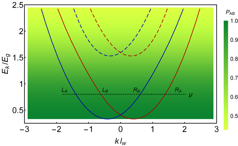
Figure 2: Energy spectrum ($E_{k}$) of a quasi-one-dimensional spin-orbit-coupled wire for $k_{\rm so}l_{w}=0.45$. The horizontal axis labels the momentum $k$ along the wire (multiplied by the wire width $l_{w}$), and the vertical axis is scaled with $E_{g}\equiv\hbar^{2}/(ml_{w}^{2})$. When the chemical potential $\mu$ (dotted line) intersects with the lowest transverse subband (solid curves) but not the upper subband (dashed curves), there exist four distinct branches, which we label as $L_{A}$, $L_{B}$, $R_{B}$, and $R_{A}$, according to their Fermi velocities. The color in the background shows the value of the spinor overlap $P_{AB}$ [see Eq. (2)].

II Hamiltonian of a clean system 

II.1 Energy spectrum and spin orientation 

Owing to their potential application in spintronics and topological matter, the spectral properties of semiconductor nanowires with spin-orbit coupling have been widely studied in the literature Moroz and Barnes (1999); Moroz et al. (2000a, b); Governale and Zülicke (2002, 2004); Braunecker et al. (2010); Meng et al. (2014); Rainis and Loss (2014); Kainaris and Carr (2015). Here we review the basic properties of a quasi-one-dimensional spin-orbit-coupled wire Moroz and Barnes (1999); Moroz et al. (2000a, b); Governale and Zülicke (2002, 2004) that are essential for our analysis. We assume that the wire lies along $x$ direction, and its transverse directions ($y$ and $z$) are subject to confinement potentials, taken as anisotropic harmonic for specificity. The $y$-axis confinement is assumed to be much softer than $z$ direction, so the $z$ transverse degrees of freedom can be neglected. The confinement energy scale $E_{g}$ is thus determined by the wire width $l_{w}$ along $y$ direction. It is known that in the presence of a relatively weak transverse confinement (meaning that $E_{g}$ is not very large), the spin-orbit coupling can cause appreciable band distortion Moroz and Barnes (1999). More precisely, the Rashba spin-orbit coupling mixes the opposite spin states of the neighboring transverse subbands, making the energy spectrum spin-dependent and distorting its originally quadratic dispersion.

Aiming at a quantitative description, we take the two-subband model introduced in Refs. Governale and Zülicke (2002, 2004). The energy spectrum depends on the dimensionless parameter $k_{\rm so}l_{w}$, with $k_{\rm so}\equiv m|\alpha_{\rm R}|/\hbar^{2}$ being determined by the Rashba coefficient $\alpha_{\rm R}$ and effective mass $m$ of the material. For the parameter values $|\alpha_{\rm R}|=$ 100–200 meVÅ, $m=0.023~{}m_{e}$ with the electron mass $m_{e}$, and $l_{w}=100~{}$nm, we obtain $k_{\rm so}l_{w}=$0.3–0.6. For illustration, Fig. 2 shows the spectrum for $k_{\rm so}l_{w}=0.45$. We label the outer (inner) branch of the energy dispersion as $A$ $(B)$ and the right- (left-)moving electron as $R$ ($L$) for the chemical potential $\mu$ located within the lowest-subband regime, as indicated in Fig. 2. Due to the band distortion induced by the spin-orbit coupling, the Fermi velocities of the branches $A$ and $B$ are different. We define the band distortion parameter as the ratio $\delta v/v_{F}$ with

$$\delta v \equiv v_{A}-v_{B},$$ (1a)

$$v_{F} \equiv (v_{A}+v_{B})/2,$$ (1b)

where $v_{A}$ ($v_{B}$) is the Fermi velocity of the branch $A$ ($B$). The band distortion parameter is plotted as a function of $\mu$ in Fig. 3. For parameters relevant to Ref. Sato et al. (2019), we obtain $\delta v/v_{F}\apprle 0.1$ in the strong-interaction regime (that is, close to the bottom of the lowest subband).

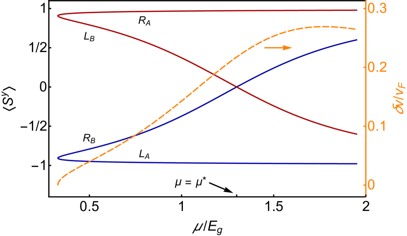
Figure 3: Chemical potential ($\mu$) dependence of the spin expectation value $\langle S^{y}\rangle$ (left axis, in unit of $\hbar/2$) of the eigenstates in the lowest subband, as well as the band distortion parameter $\delta v/v_{F}$ (right axis). For $\mu<\mu^{*}$, the spins of $R_{A}$ and $R_{B}$ are of opposite signs, so are the spins of $L_{A}$ and $L_{B}$. The adopted parameters are the same as those used in Fig. 2.

In addition to the band distortion, the spin orientation of the electrons is also affected by the spin-orbit coupling. Whereas the spins of the right- and left-moving electrons of the same branch (either $A$ or $B$) must be opposite due to the time-reversal symmetry, there is in general no relation between the spins of electrons moving in the same direction (namely, between $R_{A}$ and $R_{B}$, or, equivalently, between $L_{A}$ and $L_{B}$). In the literature, Moroz et al. assigned the electron spins of the same direction of motion as antiparallel Moroz et al. (2000a, b), while Governale and Zülicke assigned them as parallel Governale and Zülicke (2002, 2004). In fact, due to the spin-orbit mixing, the spins of $R_{A}$ and $R_{B}$ are in general neither exactly parallel nor exactly antiparallel. The relative orientation between these two spins depends on the strengths of the spin-orbit coupling and the transverse confinement, as well as the chemical potential.

To demonstrate it, in Fig. 3 we plot the $\mu$ dependence of the spin expectation values $\langle S^{y}\rangle$ with respect to the transverse wave functions of the four labeled branches. Similar to the band distortion, the spin orientation also shows strong $\mu$ dependence. Upon increasing $\mu$, the spins of $R_{A}$ and $R_{B}$ evolve from nearly antiparallel close to the bottom of the lowest subband, to not very well aligned when approaching the bottom of the upper subband. The crossover between these two regimes occurs at $\mu^{*}$, where the expectation values $\langle R_{B}|S^{y}|R_{B}\rangle$ and $\langle L_{B}|S^{y}|L_{B}\rangle$ vanish. As a result, the two sets of seemingly contradicting references (Refs. Moroz et al. (2000a, b) and Refs. Governale and Zülicke (2002, 2004)) can be reconciled–whether the former or the latter gives a better description depends on which parameter regime we are looking at. Therefore, to investigate the strong-interaction regime in Ref. Sato et al. (2019), which corresponds to the low-$\mu$ regime in Fig. 2, it is more appropriate to consider the scenario described in Refs. Moroz et al. (2000a, b).

After examining the parameter dependence of the spin orientation, we discuss the implication of the distinct spin-state assignments in Refs. Moroz et al. (2000a, b); Governale and Zülicke (2002, 2004) on our analysis. To proceed, we denote the spin states of the time-reversal pairs $R_{A}$ and $L_{A}$ as $\sigma=\uparrow$ and $\downarrow$, respectively. Similarly, the other pairs $R_{B}$ and $L_{B}$ can be labeled as $\sigma^{\prime}=\uparrow^{\prime}$ and $\downarrow^{\prime}$, respectively. As mentioned above, there is in general no relation between $\sigma$ and $\sigma^{\prime}$. Concerning transport properties, backscattering on charge impurities is feasible only between counter-propagating electrons with nonzero spinor overlap. Since the spin assignment $\sigma=\sigma^{\prime}$ in Refs. Governale and Zülicke (2002, 2004) corresponds to a helical channel, it is immune against elastic single-particle backscattering on charge impurities. To facilitate backscattering of electrons in a helical channel, an alternative mechanism has to be involved, which may arise from broken time-reversal symmetry, higher-order scattering, or inelastic process (for example, see Refs. Hsu et al. (2017, 2018) and references therein). In the present work, however, since we consider charge impurities as the dominating mechanism responsible for the transport, only backscattering processes between two non-orthogonal states (that is, $R_{A}\leftrightarrow L_{B}$ and $R_{B}\leftrightarrow L_{A}$) can cause finite resistance. In consequence, it is more appropriate to consider the spin-state assignment $\sigma=-\sigma^{\prime}$ suggested in Refs. Moroz et al. (2000a, b) for our analysis. To further quantify the backscattering strength, we compute the scalar product of two non-orthogonal states in different branches for a fixed $\mu$,

$$P_{AB} \equiv |\langle R_{A}|L_{B}\rangle|=|\langle R_{B}|L_{A}\rangle|,$$ (2)

which is shown in the background color of Fig. 2. In spite of the misaligned spins, the strength of backscattering between branches decreases only modestly when the chemical potential is increased.

Based on the above consideration, we are motivated to introduce the following fermion operators for the four branches,

$$L_{A}\to\psi_{L\downarrow},\;L_{B}\to\psi_{L\uparrow},\;R_{B}\to\psi_{R\downarrow},\;R_{A}\to\psi_{R\uparrow},$$ (3)

where we have removed the redundant prime for branch $B$. With this electron spin assignment, the energy spectrum can be linearized and the fields $\psi_{r\sigma}$ can be bosonized in the standard way [see Eq. (LABEL:Eq:bosonization) below]. The strength of the impurity-induced backscattering is affected by the spin misalignment, which influences the prefactors of the conductance and current. In our calculation, it can be incorporated through renormalized coupling constants by replacing the tunnel amplitude $t_{\rm tun}$ in Eq. (18) with (assuming that $P_{AB}$ is well above zero)

$$t_{\rm tun}^{2}\to t_{\rm tun}^{2}\Big{(}\frac{1+P_{AB}^{2}}{2}\Big{)},$$ (4)

and the backscattering strength $V_{0}$ in Eq. (45) with

$$V_{0}^{2}\to V_{0}^{2}P_{AB}^{2}.$$ (5)

Nevertheless, the spin misalignment does not affect the universal scaling exponents that we aim to determine.

In consequence, the distinct Fermi velocities of the two spin branches are symptomatic for the spin-orbit-induced band distortion discussed here, with the ratio $\delta v/v_{F}$ depending on the specific model used to compute the spectrum. In order to keep our analysis general, from now on we take $\delta v/v_{F}$ as a phenomenological parameter quantifying the band distortion effect. In the bosonized Hamiltonian, this band distortion leads to a charge-spin mixing term Moroz et al. (2000a, b), which we present in the next subsection.

II.2 Bosonized Hamiltonian 

We now present our model based on the bosonization formalism Giamarchi (2003). We introduce the Hamiltonian $H=H_{\textrm{0}}+H_{\textrm{so}}$ as a model of a clean spin-orbit-coupled wire. We postpone the discussion of additional terms induced by impurities to Sec. III. The first term, $H_{\textrm{0}}$, describes a standard, spinful Luttinger liquid

$$H_{\textrm{0}}=\sum_{\nu}\int\frac{\hbar dx}{2\pi}\left\{u_{\nu}g_{\nu}\left[\partial_{x}\theta_{\nu}(x)\right]^{2}+\frac{u_{\nu}}{g_{\nu}}\left[\partial_{x}\phi_{\nu}(x)\right]^{2}\right\}.$$ (6)

Here, $g_{\nu}$ is the interaction parameter in the $\nu$ sector (with the index $\nu\in\{c,s\}$ referring to the charge and spin sectors, respectively) and $u_{\nu}=v_{F}/g_{\nu}$ is the corresponding renormalized velocity with $v_{F}$ defined in Eq. (1). The boson fields $(\phi_{\nu},\theta_{\nu})$ are connected to the fermion fields through the standard bosonization formula,

$$\psi_{r\sigma}(x) = \frac{1}{\sqrt{2\pi a}}e^{irk_{F}x}e^{-\frac{i}{\sqrt{2}}[r\phi_{c}(x)-\theta_{c}(x)+r\sigma\phi_{s}(x)-\sigma\theta_{s}(x)]}.$$

Here, the Klein factor is omitted, $a$ is the short-distance cutoff, $k_{F}$ is the Fermi wave vector, and the index $r\in\{R\equiv+1,~{}L\equiv-1\}$ refers to the fermion operator describing the right- and left-moving particle, respectively. The boson fields satisfy the following commutation relation Giamarchi (2003),

$$\left[\phi_{\nu}(x),\theta_{\nu^{\prime}}(x^{\prime})\right] = i\frac{\pi}{2}\textrm{sign}(x^{\prime}-x)\delta_{\nu\nu^{\prime}}.$$ (8)

Equation (6) itself describes a system in which the spin-orbit-induced band distortion is absent, and reveals the separation of the charge and spin sectors, the hallmark of the standard Luttinger liquid. Throughout this article, we will constantly compare the known formula derived from Eq. (6) with our results including the influence of the band distortion.

The term $H_{\textrm{so}}$ incorporates the band distortion induced by the spin-orbit coupling Moroz and Barnes (1999); Moroz et al. (2000a, b)

$$H_{\textrm{so}}= \delta v\int\frac{\hbar dx}{2\pi}\Big{\{}\left[\partial_{x}\phi_{c}(x)\right]\left[\partial_{x}\theta_{s}(x)\right]$$

$$\hskip 42.0pt+\left[\partial_{x}\phi_{s}(x)\right]\left[\partial_{x}\theta_{c}(x)\right]\Big{\}},$$ (9)

as a mixing between the charge and spin sectors. As demonstrated in Fig. 3, the typical values of $\delta v$ are small compared to the averaged Fermi velocity $v_{F}$.

Since the Hamiltonian $H_{\textrm{0}}+H_{\textrm{so}}$ is quadratic in the boson fields, it can be diagonalized by using new boson fields,

$$\left(\begin{array}[]{c}\phi_{s}^{\prime}(x)\\ \theta_{c}^{\prime}(x)\end{array}\right) = \left(\begin{array}[]{cc}\cos\theta&-g_{0}\sin\theta\\ \frac{1}{g_{0}}\sin\theta&\cos\theta\end{array}\right)\left(\begin{array}[]{c}\phi_{s}(x)\\ \theta_{c}(x)\end{array}\right),$$ (10g)

$$\left(\begin{array}[]{c}\phi_{c}^{\prime}(x)\\ \theta_{s}^{\prime}(x)\end{array}\right) = \left(\begin{array}[]{cc}\cos\theta&g_{0}\sin\theta\\ -\frac{1}{g_{0}}\sin\theta&\cos\theta\end{array}\right)\left(\begin{array}[]{c}\phi_{c}(x)\\ \theta_{s}(x)\end{array}\right),$$ (10n)

with the parameters

$$g_{0} = \frac{\sqrt{2}g_{c}g_{s}}{\sqrt{g_{c}^{2}+g_{s}^{2}}},$$ (11a)

$$\theta = \frac{1}{2}\arctan\left(\frac{\delta v}{v_{F}}\frac{\sqrt{2}g_{c}g_{s}\sqrt{g_{c}^{2}+g_{s}^{2}}}{g_{s}^{2}-g_{c}^{2}}\right).$$ (11b)

It can be checked that these new boson fields satisfy the commutation relation (8) upon replacing the fields $(\phi_{\nu},\theta_{\nu})\rightarrow(\phi_{\nu}^{\prime},\theta_{\nu}^{\prime})$. In terms of the new fields, the Hamiltonian reads

$$H = \sum_{\nu}\int\frac{\hbar dx}{2\pi}\left\{u_{\nu}^{\prime}g_{\nu}^{\prime}\left[\partial_{x}\theta_{\nu}^{\prime}(x)\right]^{2}+\frac{u_{\nu}^{\prime}}{g_{\nu}^{\prime}}\left[\partial_{x}\phi_{\nu}^{\prime}(x)\right]^{2}\right\},$$

where the modified interaction parameters and velocities by the spin-orbit coupling are given by

$$g_{c}^{\prime} = \frac{g_{c}g_{0}}{g_{s}}\left[\frac{g_{s}^{2}-(g_{0}^{2}+g_{s}^{2})\sin^{2}\theta}{g_{0}^{2}-(g_{0}^{2}+g_{c}^{2})\sin^{2}\theta}\right]^{1/2},$$ (13a)

$$g_{s}^{\prime} = \frac{g_{s}g_{0}}{g_{c}}\left[\frac{g_{c}^{2}-(g_{0}^{2}+g_{c}^{2})\sin^{2}\theta}{g_{0}^{2}-(g_{0}^{2}+g_{s}^{2})\sin^{2}\theta}\right]^{1/2},$$ (13b)

and

$$u_{c}^{\prime} = \frac{u_{c}}{g_{0}g_{s}\cos(2\theta)}\left[g_{0}^{2}-(g_{0}^{2}+g_{c}^{2})\sin^{2}\theta\right]^{1/2}$$ (13c)

$$\hskip 48.0pt\times\left[g_{s}^{2}-(g_{0}^{2}+g_{s}^{2})\sin^{2}\theta\right]^{1/2},$$

$$u_{s}^{\prime} = \frac{u_{s}}{g_{0}g_{c}\cos(2\theta)}\left[g_{0}^{2}-(g_{0}^{2}+g_{s}^{2})\sin^{2}\theta\right]^{1/2}$$ (13d)

$$\hskip 48.0pt\times\left[g_{c}^{2}-(g_{0}^{2}+g_{c}^{2})\sin^{2}\theta\right]^{1/2},$$

respectively. In the absence of spin-orbit coupling (that is, when $\delta v,~{}\theta\rightarrow 0$), we recover the limit $(g_{c}^{\prime},g_{s}^{\prime},u_{c}^{\prime},u_{s}^{\prime})\rightarrow(g_{c},g_{s},u_{c},u_{s})$, as expected. The above formulas quantify the effects of the band distortion, Eq. (9), on the interaction parameters and velocities. For fixed $\delta v$, the parameters $\theta$ and $g_{0}$ decrease with a decreasing $g_{c}$. Therefore, $g_{\nu}^{\prime}$ approaches its value at zero spin-orbit coupling ($g_{\nu}$) when $g_{c}$ approaches zero. As a result, the modification of the interaction parameters by the band distortion is smaller for more strongly interacting wires.

For a moderate strength of the interaction, since the modified interaction parameters enter the exponents of the correlation functions, we expect to see influence on observable quantities. In particular, we are interested in the charge transport of a spin-orbit-coupled wire for arbitrary strength of interaction. Since the ballistic conductance of a clean spin-orbit-coupled system displays no signature for a Luttinger liquid Moroz et al. (2000b), as originally found for systems without spin-orbit coupling Maslov and Stone (1995); Ponomarenko (1995); Safi and Schulz (1995), in the following we seek for signatures in the presence of impurities.

III Transport properties in the presence of various impurities 

We aim at finding out how the charge-spin mixing term in Eq. (9) influences the transport properties of the system. To this end, we compute the current and/or the differential conductance of the system described by Eq. (LABEL:Eq:diag) in the presence of various types of impurities illustrated in Fig. 1. We consider a wire adiabatically connected to the leads, a common assumption as in, e.g., Refs. Ponomarenko (1995); Maslov (1995); Sandler and Maslov (1997); Egger and Grabert (1998); Aseev et al. (2018); for the effect of an abrupt contact in a microscopic model, see Refs. Meden et al. (2003); Janzen et al. (2006).

III.1 Strong impurities–tunnel barriers 

We begin with an isolated strong impurity and model it as a weak tunnel barrier. Assuming that the barrier is located at the origin, the two sides of the barrier are described by

$$H_{1}= \sum_{\nu}\int_{-\infty}^{0}\frac{\hbar u_{1\nu}^{\prime}dx}{2\pi}\;\left\{g_{1\nu}^{\prime}\left[\partial_{x}\theta_{1\nu}^{\prime}(x)\right]^{2}+\frac{\left[\partial_{x}\phi_{1\nu}^{\prime}(x)\right]^{2}}{g_{1\nu}^{\prime}}\right\},$$ (14a)

$$H_{2}= \sum_{\nu}\int_{0}^{\infty}\frac{\hbar u_{2\nu}^{\prime}dx}{2\pi}\;\left\{g_{2\nu}^{\prime}\left[\partial_{x}\theta_{2\nu}^{\prime}(x)\right]^{2}+\frac{\left[\partial_{x}\phi_{2\nu}^{\prime}(x)\right]^{2}}{g_{2\nu}^{\prime}}\right\},$$ (14b)

obtained by generalizing Eq. (LABEL:Eq:diag) to possibly different parameters on the two sides. We include an additional index $j\in\{1,2\}$ to label the semi-infinite subsystem on the left and right side of the barrier, respectively. The two subsystems are connected through a tunneling process described by

$$H_{\rm tun}=-t_{\rm tun}\sum_{\sigma}c_{1\sigma}^{\dagger}c_{2\sigma}+{\rm H.c.},$$ (15)

where $t_{\rm tun}$ is the tunnel amplitude and $c_{j\sigma}$ is the fermion operator with spin $\sigma\in\{\uparrow,\downarrow\}$ at $x=0$ in the left ($j=1$) or right ($j=2$) side. It is related to the right- and left-movers in Eq. (LABEL:Eq:bosonization) by

$$c_{j\sigma}=\psi_{jR\sigma}(0)+\psi_{jL\sigma}(0),$$ (16)

where we generalize the field in Eq. (LABEL:Eq:bosonization) to $\psi_{jr\sigma}$ by including the subsystem index $j$.

The tunnel current through the barrier depends on whether the barrier is located near the boundary or in the bulk of the wire. When it is near the boundary, the barrier corresponds to a junction between a Luttinger liquid wire and a Fermi-liquid lead. In this case, one side of the barrier (say, for $x<0$) is described by the parameters of a lead with negligible interaction such that $(g_{1c}^{\prime},~{}g_{1s}^{\prime})=(1,~{}1)$, whereas on the other side (for $x>0$) the wire parameters are $(g_{2c}^{\prime},~{}g_{2s}^{\prime})=(g_{c}^{\prime},~{}g_{s}^{\prime})$. When the barrier is in the bulk of the wire, on the other hand, the barrier corresponds to a junction between two Luttinger liquids. Therefore, both $H_{1}$ and $H_{2}$ have parameters $(g_{1c}^{\prime},~{}g_{1s}^{\prime})=(g_{2c}^{\prime},~{}g_{2s}^{\prime})=(g_{c}^{\prime},~{}g_{s}^{\prime})$. In the following, we first keep general parameters for the two subsystems $j$, and specify them later.

To the leading order, the tunnel current through the barrier is given by Schrieffer et al. (1963); Wen (1991)

$$I=\frac{et_{\rm tun}^{2}}{\hbar^{2}}\sum_{\sigma}\int_{0}^{\infty}dt\;\Big{\{}e^{-ieVt/\hbar}\Big{\langle}\Big{[}c_{1\sigma}^{\dagger}(t)c_{2\sigma}(t),c_{2\sigma}^{\dagger}(0)c_{1\sigma}(0)\Big{]}\Big{\rangle}-e^{ieVt/\hbar}\Big{\langle}\Big{[}c_{2\sigma}^{\dagger}(t)c_{1\sigma}(t),c_{1\sigma}^{\dagger}(0)c_{2\sigma}(0)\Big{]}\Big{\rangle}\Big{\}},$$ (17)

with the elementary charge $e$, the reduced Planck constant $\hbar$, and the voltage difference $V$ between the two sides of the barrier. Here, the notation $[\cdots,\cdots]$ is the commutator and $\langle\cdots\rangle$ is the average with respect to the unperturbed action [before introducing Eq. (15)]. It is convenient to write Eq. (17) as

$$I= -\frac{2et_{\rm tun}^{2}}{\hbar^{2}}\sum_{\sigma}{\rm Im}\Big{[}\chi_{\sigma}^{\rm ret}(-eV/\hbar)\Big{]},$$ (18)

with ${\rm Im}[\cdots]$ being the imaginary part and the following correlation functions,

$$\chi_{\sigma}^{\rm ret}(\omega) \equiv -i\int_{0}^{\infty}dt\;e^{i\omega t}\Big{[}\chi_{\sigma}(t)-\chi_{\sigma}(-t)\Big{]},$$ (19a)

$$\chi_{\sigma}(t) \equiv \Big{\langle}c_{1\sigma}^{\dagger}(t)c_{1\sigma}(0)\Big{\rangle}_{1}\Big{\langle}c_{2\sigma}(t)c_{2\sigma}^{\dagger}(0)\Big{\rangle}_{2},$$ (19b)

where $\langle\cdots\rangle_{j}$ is the average corresponding to $H_{j}$ in Eq. (14).

The single-particle equal-space correlation function in the above formula is defined at the boundary of the Luttinger liquid. To take the boundary into account properly, we treated it along the lines of Ref. Giamarchi (2003), as presented in Appendix A. At finite temperature $T$, the single-particle correlation function is

$$\Big{\langle}c_{j\sigma}^{\dagger}(t)c_{j\sigma}(0)\Big{\rangle}_{j} = \frac{1}{2\pi a}\sum_{r=\pm}\Big{[}\frac{\pi k_{B}T/\Delta_{a}}{i\sinh(\pi k_{B}Tt/\hbar)}\Big{]}^{\beta_{jr\sigma}+1},$$

with the Boltzmann constant $k_{B}$ and the bandwidth $\Delta_{a}\equiv\hbar v_{F}/a$. The exponent $\beta_{jr\sigma}$, given in Eq. (64), corresponds to the density of states at the boundary of the subsystem $j$. Plugging the above formula into Eq. (19), with some algebra and approximations presented in Appendix B, we get the current-voltage curve at finite temperature as

$$I \propto T^{\alpha+1}\sinh\left(\frac{eV}{2k_{B}T}\right)\left|\Gamma\left(1+\frac{\alpha}{2}+i\frac{eV}{2\pi k_{B}T}\right)\right|^{2},$$

with the gamma function $\Gamma(x)$. The current-voltage relation has the same form as in Ref. Balents (1999) except for a parameter modified by the spin-orbit coupling,

$$\alpha=\alpha_{1}+\alpha_{2}.$$ (22)

The explicit form of $\alpha_{j}$ depends on the density of states on the two sides of the barrier and thus the location of the barrier, which will be specified later.

So far we have considered a wire with a single barrier which causes a voltage drop $V$. As discussed in Ref. Bockrath et al. (1999), assuming that there are $N_{\rm b}$ independent barriers in the wire, each of which causes a similar voltage drop with $V$ being the bias voltage across the entire wire, Eq. (LABEL:Eq:Balents) is valid upon replacing $V\rightarrow V/N_{\rm b}$. Here, the barrier number $N_{\rm b}$ corresponds to the parameter $\gamma=1/N_{\rm b}$ in Refs. Bockrath et al. (1999); Sato et al. (2019). As a result, it is possible to experimentally determine the number of the barriers in the wire through the current-voltage characteristics.

Before specifying the barrier type to obtain the exponent in Eq. (22) in terms of the parameters in Eqs. (11) and (13), we make four remarks on Eqs. (LABEL:Eq:Balents)–(22). First, the current-voltage curve exhibits a universal scaling behavior, analogous to the zero spin-orbit coupling case Balents (1999). Namely, the rescaled current, $I/T^{\alpha+1}$, is a function of the ratio $V/T$. Therefore, the curves $I/T^{\alpha+1}$ plotted versus $V/T$ for various bias voltages and temperatures collapse onto a single curve.

Second, in addition to the full dependence on the temperature and bias voltage, the asymptotic behavior of the (differential) conductance $G\equiv dI/dV$ may be of interest. In the $eV\ll k_{B}T$ regime, Eq. (LABEL:Eq:Balents) gives the linear-response conductance with a power-law temperature dependence, whereas in the opposite limit we find a nonlinear current-voltage curve; the detailed discussions on the asymptotic behavior of Eq. (LABEL:Eq:Balents) are presented in Appendix B. The behavior in these limits can be summarized as

$$G\equiv\frac{dI}{dV} \propto \left\{\begin{array}[]{l}T^{\alpha},\;\;{\rm for}\;\;eV\ll k_{B}T,\\ V^{\alpha},\;\;{\rm for}\;\;eV\gg k_{B}T,\end{array}\right.$$ (25)

that is, a power-law conductance with the identical exponent $\alpha$ in the high-temperature and high-bias regimes.

Third, the value of $\alpha$, which parametrizes the universal scaling relation Eq. (LABEL:Eq:Balents), depends on the interaction parameters, so that the current-voltage curve can be used to extract the strength of the electron-electron interaction in the wire. Such characterization, however, strongly depends on the location of the barrier, as discussed below.

Finally, it may be tempting to guess the parameter $\alpha$ in Eq. (22) using the corresponding form in the absence of the spin-orbit coupling. Namely, one may naively replace $(g_{c},g_{s})\rightarrow(g_{c}^{\prime},g_{s}^{\prime})$ in the following expressions Kane and Fisher (1992b); Furusaki and Nagaosa (1993); Matveev and Glazman (1993)

$$\alpha_{\rm end}(\delta v=0) = \frac{1}{2g_{c}}+\frac{1}{2g_{s}}-1,$$ (26a)

$$\alpha_{\rm bulk}(\delta v=0) = \frac{1}{g_{c}}+\frac{1}{g_{s}}-2,$$ (26b)

for boundary and bulk barriers, respectively. Such a replacement would, however, have given an incorrect result. The reason can be traced back to the fact that the tunnel Hamiltonian is written with the original fermions. When expressing these fermions in terms of the new fields $\phi_{\nu}^{\prime}$ and $\theta_{\nu}^{\prime}$, additional coefficients arise from the transformation from the fields $\phi_{\nu}$ and $\theta_{\nu}$ into the new ones using Eq. (10). As a result, $\alpha$ as a function of $g_{c}^{\prime}$ and $g_{s}^{\prime}$ has a different functional than Eqs. (26), as we now demonstrate.

Let us consider the boundary barrier, so that there is a noninteracting lead to the left ($j=1$) and a spin-orbit-coupled Luttinger liquid to the right ($j=2$) of the barrier, as illustrated in Fig. 1(a). With the exponent of the single-particle correlation function $\alpha_{j}$ derived in Appendix B, we obtain the current-voltage curve Eq. (LABEL:Eq:Balents), with $\alpha$ given by

$$\alpha_{\rm end} = \frac{1}{2}\left(\frac{1}{g_{c}^{\prime}}+\frac{1}{g_{s}^{\prime}}\right)\left(\cos^{2}\theta+g_{0}^{2}\sin^{2}\theta\right)-1.$$ (27)

It goes over to Eq. (26) in the limit of $\delta v$, $\theta\rightarrow 0$.

We now turn to the case in which the tunnel barrier is located in the bulk of the wire. The tunneling process corresponds to a particle transiting from the boundary of a Luttinger liquid into the boundary of the other, as illustrated in Fig. 1(b). It gives rise to a current-voltage curve of the form of Eq. (LABEL:Eq:Balents) again, but with a different exponent, namely

$$\alpha_{\rm bulk} = \left(\frac{1}{g_{c}^{\prime}}+\frac{1}{g_{s}^{\prime}}\right)\left(\cos^{2}\theta+g_{0}^{2}\sin^{2}\theta\right)-2.$$ (28)

Again, Eq. (26) follows for $\delta v$, $\theta\rightarrow 0$. Comparing to Eq. (27), we see that $\alpha_{\rm bulk}$ is twice of $\alpha_{\rm end}$. The exponent can be expanded in series of $\sin\theta$. In the leading order, the spin-orbit-induced change is

$$\alpha_{\rm bulk}-\alpha_{\rm bulk}(\delta v=0)\approx-\frac{(g_{c}+g_{s})\sin^{2}\theta}{4g_{c}^{2}g_{s}^{2}(g_{c}^{2}+g_{s}^{2})}$$

$$\hskip 36.135pt\times\Big{[}(g_{c}^{2}-g_{s}^{2})^{2}+4g_{c}g_{s}\big{(}g_{c}^{2}+g_{s}^{2}-2g_{c}^{2}g_{s}^{2}\big{)}\Big{]}.$$ (29)

For $g_{c}$ not close to $g_{s}$, we can further express it in terms of the intrinsic interaction and band distortion parameters. We get, up to second order in $\delta v/v_{F}$,

$$\alpha_{\rm bulk}-\alpha_{\rm bulk}(\delta v=0)$$

$$\approx -\frac{\delta v^{2}(g_{c}+g_{s})}{8v_{F}^{2}}\Big{[}1+\frac{4g_{c}g_{s}}{(g_{c}^{2}-g_{s}^{2})^{2}}\big{(}g_{c}^{2}+g_{s}^{2}-2g_{c}^{2}g_{s}^{2}\big{)}\Big{]}.$$

For $g_{c}$ close to $g_{s}$ (including the noninteracting limit), on the other hand, the coefficient of the above expression diverges, so the approximation is inaccurate close to this limit. Nonetheless, Eq. (LABEL:Eq:alpha_bulk_approx) is a good approximation when the electron-electron interaction is sufficiently strong, say for $g_{c}\apprle 0.7$ and $g_{s}=1$.

To demonstrate how Eqs. (27) and (28) depend on the band distortion, we plot in Fig. 4 the $g_{c}$ dependence of the $\delta v$-induced change $\Delta\alpha_{\rm bulk}\equiv\alpha_{\rm bulk}-\alpha_{\rm bulk}(\delta v=0)$ for several values of $\delta v/v_{F}$, as well as the zero-spin-orbit value of the exponent $\alpha_{\rm bulk}$. As shown in Fig. 4(a), the parameter $\alpha_{\rm bulk}(\delta v=0)$ [see Eq. (26)] increases with a decreasing $g_{c}$. In other words, the suppression of the power-law conductance at low energies is stronger for systems with stronger interaction, a feature of the standard Luttinger liquid Kane and Fisher (1992b); Furusaki and Nagaosa (1993). For a nonzero $\delta v$, there is a non-monotonic change in $\alpha_{\rm bulk}$, as shown in Fig. 4(b). For parameters of Ref. Sato et al. (2019), the small value of $\delta v/v_{F}\apprle 0.1$ leads to negligible changes $\Delta\alpha_{\rm bulk}$. We include also larger values of $\delta v/v_{F}$, which are relevant for nanowires with weaker transverse confinement or stronger spin-orbit coupling. However, even with an exaggerated value of $\delta v/v_{F}=0.6$, one can see that the change $\Delta\alpha_{\rm bulk}$ for small $g_{c}$ is small compared to its zero-spin-orbit value [the opposite value of $\alpha_{\rm bulk}(\delta v=0)$ is plotted in Fig. 4(b) for comparison]. It means that in the strong-interaction regime even very strong band distortion leads to negligible effects on the current-voltage curves. On the other hand, in the moderate-interaction regime where the band distortion does modify the parameters, $\alpha_{\rm bulk}$ decreases (rather than increases) upon increasing the degree of the band distortion. These features were the main argument for our conclusion in Ref. Sato et al. (2019) that the large extracted $\alpha$ values from the experimental data indeed reflect the strong electron-electron interaction in the system, instead of arising from strong spin-orbit coupling of InAs nanowires.

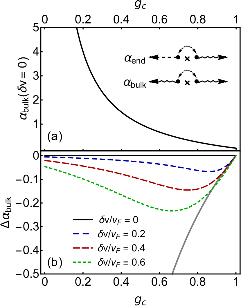
Figure 4: (a) Interaction parameter ($g_{c}$) dependence of the bulk parameter ($\alpha_{\rm bulk}$) for $g_{s}=1$ and $\delta v=0$. The parameter $\alpha_{\rm bulk}$ or $\alpha_{\rm end}$ characterizes the current-voltage curve Eq. (LABEL:Eq:Balents) and the power-law conductance given in Eq. (25) for a bulk or end barrier, where the subscripts specify the barrier types illustrated in the inset, corresponding to Panels (a) and (b) of Fig. 1. The associated parameter $\alpha_{\rm end}$ ($\alpha_{\rm bulk}$) is given in Eq. (27) [Eq. (28)]. These two are related to each other by $\alpha_{\rm bulk}=2\alpha_{\rm end}$. (b) Interaction parameter ($g_{c}$) dependence of the change ($\Delta\alpha_{\rm bulk}$) due to the spin-orbit-induced band distortion $\delta v/v_{F}$ for $g_{s}=1$. The inverse of $\alpha_{\rm bulk}$ from Panel (a) is plotted in gray.

Here, we additionally point out that, in general, the change $\Delta\alpha$ of the parameter can be sizable compared to its zero-spin-orbit value $\alpha(\delta v=0)$. As an example, for $\delta v/v_{F}=0.1$ and $g_{c}=0.9$ we obtain $\Delta\alpha/\alpha(\delta v=0)\approx-27~{}\%$, which could be observable. As displayed in Fig. 4, for $g_{c}$ even closer to unity, the magnitude of the correction can be comparable with the zero-spin-orbit value, resulting in a vanishing exponent. This feature implies that, for weakly interacting systems, the spin-orbit coupling can quench the transport signature for a Luttinger liquid subject to tunnel barriers. Overall, we expect that the band-distortion effects found here become most significant in the moderate-interaction regime or even weak-(but finite-)interaction regime.

We now employ an alternative, renormalization-group (RG), approach Giamarchi (2003); Kane and Fisher (1992b); Furusaki and Nagaosa (1993) to compute the conductance. To this end, we derive the RG flow equation for the tunnel amplitude, which is related to the scaling dimension of the equal-space correlation function at the origin. Following a similar procedure as presented in Appendices A and B, we get

$$\frac{d\tilde{t}(\ell)}{d\ell} = -\frac{1}{2}\Big{(}\alpha_{1}+\alpha_{2}\Big{)}\tilde{t}(\ell),$$ (31)

with the dimensionless tunnel amplitude $\tilde{t}(\ell)\equiv t_{\rm tun}(\ell)/\Delta_{a}(\ell)$ and dimensionless length scale defined through $a(\ell)=a(0)e^{\ell}$. Since for repulsive interaction the parameter $\alpha_{1}+\alpha_{2}$ is positive, the tunnel amplitude flows to zero, implying an insulating phase at low energies. However, to get the relevant solution, the RG flow equations should be stopped at a scale $\ell^{*}$ associated with the shorter of $\ln[\Delta_{a}/(k_{B}T)]$ and $\ln[\Delta_{a}/(eV)]$. The conductance through the tunnel barrier is obtained by integrating the RG flow up to the scale $\ell^{*}$, leading to

$$G \propto \frac{2e^{2}}{h}\left[\tilde{t}(\ell^{*})\right]^{2}\propto\big{[}{\rm Max}(eV,k_{B}T)\big{]}^{\alpha_{1}+\alpha_{2}},$$ (32)

which holds for both types of barriers.

We now specify the barrier type. For a boundary barrier, the conductance is given by

$$G_{\rm end}(T,V) \propto \left\{\begin{array}[]{l}T^{\alpha_{\rm end}},\;\;{\rm for}\;\;eV\ll k_{B}T,\\ V^{\alpha_{\rm end}},\;\;{\rm for}\;\;eV\gg k_{B}T,\end{array}\right.$$ (35)

which is consistent with both the high-temperature and the high-bias behavior of Eq. (LABEL:Eq:Balents). Similarly, for a tunnel barrier in the bulk, we get

$$G_{\rm bulk}(T,V) \propto \left\{\begin{array}[]{l}T^{\alpha_{\rm bulk}},\;\;{\rm for}\;\;eV\ll k_{B}T,\\ V^{\alpha_{\rm bulk}},\;\;{\rm for}\;\;eV\gg k_{B}T,\end{array}\right.$$ (38)

again consistent with the tunnel current. The result that the RG approach gives the same power-law conductance as the tunnel current approach should not be surprising: both of them are essentially calculating the density of states at both sides of a barrier. Compared to the tunnel current, the RG approach gives only the asymptotic behavior of the conductance (in certain limits and without prefactors). On the other hand, it can be used to compute the conductance in the case of weak impurities, where the other method is not feasible.

III.2 Weak impurities–potential disorder 

We now consider the transport properties in the presence of weak impurities, each of which acts as a backscattering center. Accordingly, we retain Eq. (LABEL:Eq:diag) for the entire wire. Let us consider first one of such impurities at the origin, as illustrated in Fig. 1(c). We model it as generating a delta-like potential

$$V_{\rm imp}(x) = V_{0}\delta(x),$$ (39)

with the strength $V_{0}$ and the Dirac delta function $\delta(x)$. By coupling to the charge density, it leads to the following term,

$$H_{\rm imp} = \sum_{rr^{\prime}\sigma}\int dx\;V_{\rm imp}(x)\left[\psi_{r\sigma}^{\dagger}(x)\psi_{r^{\prime}\sigma}(x)\right]$$ (40)

$$\approx \frac{2V_{0}}{\pi a}\cos[\sqrt{2}\phi_{c}(0)]\cos[\sqrt{2}\phi_{s}(0)],$$

where in the second line we keep only the backscattering term, as the forward scattering does not affect the conductance. The above term contributes to the second-order terms of the effective action in $V_{0}$ Kane and Fisher (1992b); Furusaki and Nagaosa (1993); Giamarchi (2003), from which we derive the RG flow equation for the backscattering strength,

$$\frac{d\tilde{V}_{0}(\ell)}{d\ell} = \frac{\alpha_{\rm imp}}{2}\tilde{V}_{0}(\ell).$$ (41)

In the above, we introduce the dimensionless coupling constant $\tilde{V}_{0}(\ell)\equiv V_{0}(\ell)/\Delta_{a}(\ell)$ and the parameter

$$\alpha_{\rm imp} = 2-\left[\cos^{2}\theta(g_{c}^{\prime}+g_{s}^{\prime})+g_{0}^{2}\sin^{2}\theta\left(\frac{1}{g_{c}^{\prime}}+\frac{1}{g_{s}^{\prime}}\right)\right].$$

In the absence of spin-orbit coupling, it becomes $\alpha_{\rm imp}(\delta v=0)=2-g_{c}-g_{s}$, consistent with Refs. Kane and Fisher (1992b); Furusaki and Nagaosa (1993); Maslov (1995). Up to the second order in $\sin\theta$, we get

$$\alpha_{\rm imp}-\alpha_{\rm imp}(\delta v=0)$$ (43)

$$\approx -\frac{\sin^{2}\theta(g_{c}+g_{s})(g_{c}-g_{s})^{4}}{4g_{c}^{2}g_{s}^{2}(g_{c}^{2}+g_{s}^{2})}\big{(}g_{c}^{2}+g_{s}^{2}+3g_{c}g_{s}\big{)}.$$

In terms of the intrinsic parameters, we derive the following approximate formulas for the change of $\alpha_{\rm imp}$,

$$\alpha_{\rm imp}(\delta v)-\alpha_{\rm imp}(0)\approx-\frac{\delta v^{2}}{8v_{F}^{2}}\frac{(g_{s}-g_{c})^{2}}{g_{c}+g_{s}}\big{(}g_{c}^{2}+g_{s}^{2}+3g_{c}g_{s}\big{)}.$$ (44)

In contrast to Eq. (LABEL:Eq:alpha_bulk_approx), the divergence upon expanding $\sin^{2}\theta\propto(g_{c}-g_{s})^{-2}$ is eliminated by the factor $(g_{c}-g_{s})^{4}$ in Eq. (43). As a result, the above approximation holds also for $g_{c}\approx g_{s}$, including the noninteracting limit.

We now comment on the RG flow equation (41). For repulsive interaction we have $\alpha_{\rm imp}>0$, so that the backscattering strength grows under the RG flow. Therefore, a single weak impurity gives rise to the conductance correction $\delta G_{\rm 1}$, with

$$\frac{\delta G_{\rm 1}}{G_{0}} \propto -\tilde{V}^{2}_{0}(\ell^{*})\sim-\tilde{V}^{2}_{0}(0)e^{\ell^{*}\alpha_{\rm imp}},$$ (45)

with the conductance quantum $G_{0}=2e^{2}/h$. The scale $\ell^{*}$, again, depends on other parameters, which we specify later.

Before moving on to the discussion of the many-impurity case, we have a few comments on the above result. First, with the RG approach we construct two flow equations–one for the tunnel amplitude $\tilde{t}$ derived for a tunnel barrier and the other for the backscattering strength $\tilde{V}_{0}$ derived for a weak impurity. For repulsive interaction, the former equation [Eq. (31)] indicates that the tunnel amplitude is RG irrelevant and flows toward zero, so the two semi-infinite Luttinger liquids become isolated at low energies. The same conclusion follows from Eq. (41), where the backscattering strength increases under the RG flow, so that the conductance is suppressed by repulsive interaction. As a consequence, the RG approach provides consistent results for the two complementary limits of impurities, as in the absence of the spin-orbit coupling Voit (1995); Giamarchi (2003).

Second, in contrast to a standard Luttinger liquid, the presence of the spin-orbit coupling defies the duality mapping between a bulk barrier and a weak impurity. Namely, in the absence of the spin-orbit coupling, the corresponding RG flow equations [see Eqs. (31) and (41)] can be mapped into each other upon swapping the parameters $g_{\nu}\leftrightarrow 1/g_{\nu}$ Furusaki and Nagaosa (1993). In a spin-orbit-coupled wire, however, such a duality mapping is absent.

We now demonstrate how a power-law conductance can arise in the scenario of many weak impurities, relevant for a wire much longer than the average impurity separation. We assume that these impurities can be treated as independent (see Appendix D for a discussion of this assumption) and each of them causes a conductance correction as computed above. Namely, the RG flow for $\tilde{V}_{0}$ is integrated up to the scale $\ell^{*}$, leading to the wire conductance in the presence of a single weak impurity

$$G_{0}+\delta G_{\rm 1} = G_{0}-c_{\rm 1}G_{0}\Big{[}\frac{\Delta_{a}}{{\rm Max}(k_{B}T,eV)}\Big{]}^{\alpha_{\rm imp}},$$ (46)

with a dimensionless constant $c_{\rm 1}$ independent of temperature and voltage. From Eq. (46), we obtain the resistance induced by a single impurity,

$$\delta R_{\rm 1}\approx-\frac{\delta G_{\rm 1}}{G_{0}^{2}}\propto\big{[}{\rm Max}(k_{B}T,eV)\big{]}^{-\alpha_{\rm imp}}.$$ (47)

If there are $N_{\rm imp}$ impurities in the wire, adding their resistances in series gives the total resistance as $1/G_{0}+N_{\rm imp}\delta R_{\rm 1}$ with the lead-wire contact resistance $1/G_{0}$. For large $N_{\rm imp}$, the total resistance (defined as $1/G_{\rm imp}$) is dominated by the contribution from the impurities (so that the contact resistance is negligible), leading to

$$G_{\rm imp}(T,V) \propto \left\{\begin{array}[]{l}T^{\alpha_{\rm imp}},\;\;{\rm for}\;\;eV\ll k_{B}T,\\ V^{\alpha_{\rm imp}},\;\;{\rm for}\;\;eV\gg k_{B}T,\end{array}\right.$$ (50)

which is a power law with the same exponent in the high-temperature and high-bias regimes.

Importantly, the two power laws in the opposite limits with the same exponent can be grasped by a single function using Eq. (LABEL:Eq:Balents) upon replacing the parameter $\alpha$ by $\alpha_{\rm imp}$. In other words, we take Eq. (LABEL:Eq:Balents) as an interpolation formula valid for arbitrary bias and temperature. It can be then used as the fitting curve of data displaying universal scaling. In this many-weak-impurity scenario, the variable $V$ denotes the bias voltage across the entire wire. In contrast to the tunnel barrier scenario, where the replacement $V\rightarrow V/N_{\rm b}$ in Eq. (LABEL:Eq:Balents) is necessary for multiple barriers, here Eq. (LABEL:Eq:Balents) remains unchanged regardless of the number of weak impurities.

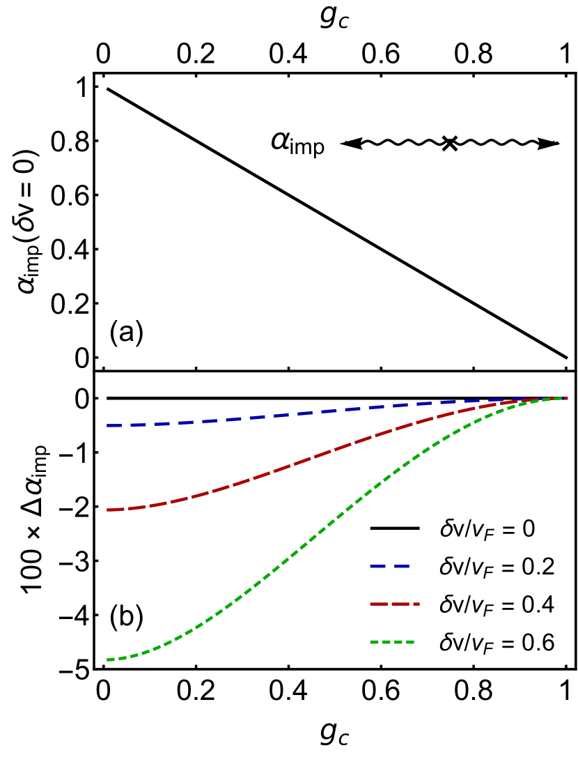
Figure 5: (a) Interaction parameter ($g_{c}$) dependence of the parameter ($\alpha_{\rm imp}$) for $g_{s}=1$ and $\delta v=0$. The inset illustrates a weak impurity corresponding to Fig. 1(c). Many such weak impurities cause a power-law conductance [see Eq. (50)] with the exponent $\alpha_{\rm imp}$ defined in Eq. (LABEL:Eq:alpha_imp). (b) Interaction parameter ($g_{c}$) dependence of the change ($\Delta\alpha_{\rm imp}$, multiplied by 100 for clarity) of the exponent $\alpha_{\rm imp}$ with respect to its value for $\delta v=0$ for $g_{s}=1$ and several values of $\delta v/v_{F}$.

In Fig. 5, we plot the exponent $\alpha_{\rm imp}$ at zero spin-orbit coupling and its change $\Delta\alpha_{\rm imp}$ for several values of $\delta v/v_{F}$ as functions of $g_{c}$. Similar to Fig. 4, the exponent $\alpha_{\rm imp}$ for $\delta v=0$ [see Fig. 5(a)] increases with a larger strength of the interaction (that is, a smaller $g_{\rm c}$ value), and the band distortion can only reduce $\alpha_{\rm imp}$ [see Fig. 5(b)]. In comparison with Fig. 4, on the other hand, the effect of the band distortion on the exponent $\alpha_{\rm imp}$ is quantitatively much weaker. Moreover, in contrast to Fig. 4, where $\alpha_{\rm end}$ and $\alpha_{\rm bulk}$ are unbounded in the strong-interaction regime, the corresponding parameter for weak impurities is bounded in the range $\alpha_{\rm imp}\in[0,1]$. Therefore, it is possible to rule out weak impurities as the dominant resistance contribution if the $\alpha$ value extracted from the current-voltage measurements exceeds unity. Furthermore, if both types of impurities are present, the resistance due to tunnel barriers dominates weak impurities for strong interaction, while the relation is opposite for weak interaction. Therefore, we predict a transition of the power-law conductance by varying electron-electron interaction, as discussed below.

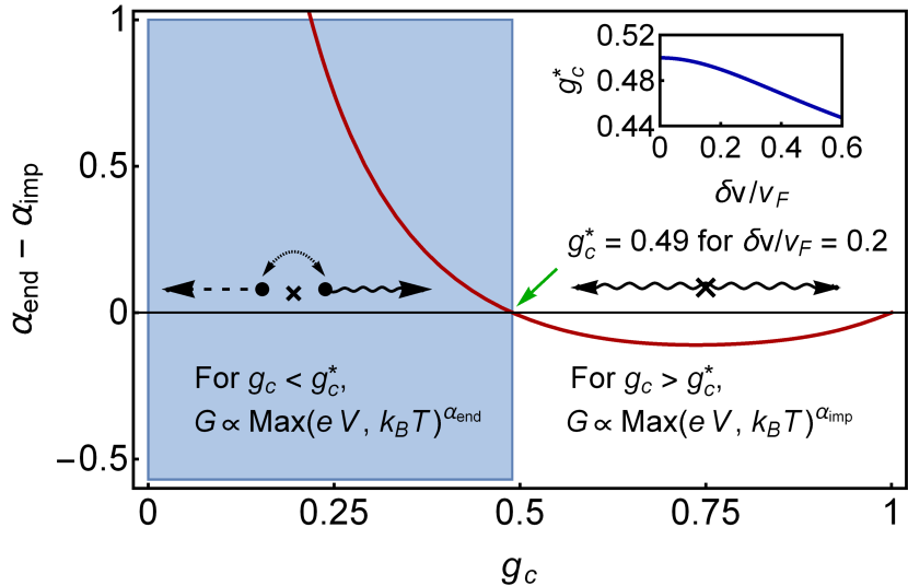
Figure 6: Transition of the power-law conductance. The main panel shows the difference $(\alpha_{\rm end}-\alpha_{\rm imp})$ as a function of the interaction parameter $(g_{c})$ for $g_{s}=1$ and $\delta v/v_{F}=0.2$. The exponents $\alpha_{\rm end}$ and $\alpha_{\rm imp}$ are given in Eqs. (27) and (LABEL:Eq:alpha_imp), respectively. The point at which $\alpha_{\rm end}=\alpha_{\rm imp}$ (denoted as $g_{c}^{*}$) indicates a transition between the regimes with different power-law conductance. For $g_{c}<g_{c}^{*}$ (blue shaded region), the power-law conductance is characterized by $\alpha_{\rm end}$, whereas for $g_{c}>g_{c}^{*}$ it is characterized by $\alpha_{\rm imp}$. The inset shows the dependence of $g_{c}^{*}$ value on $\delta v/v_{F}$.

III.3 Coexisting strong and weak impurities 

Here we discuss the scenario in which impurities of all the types are present. Provided that the effects of the tunnel barriers and weak impurities on the resistance do not interfere with each other so that each resistance source can be treated separately as in Secs. III.1 and III.2, their contributions can be added into the total resistance of the entire wire. In general, the three resistance sources [corresponding to Eqs. (35), (38), and (50)] enter the total resistance as

$$R_{\rm tot} \propto \frac{h}{2e^{2}}\sum_{n}c_{n}\big{[}\frac{\Delta_{a}}{{\rm Max}(eV,k_{B}T)}\big{]}^{\alpha_{n}},$$ (51)

where $n\in\{{\rm end},~{}{\rm bulk},~{}{\rm imp}\}$ indicates the resistance source. In the above, $c_{n}$’s are the corresponding prefactors. Since in typical experiments we have $\Delta_{a}\gg eV,k_{B}T$, the total resistance of a wire is dominated by the contribution with the largest exponent. Therefore, for any repulsive interaction, as long as there exists a tunnel barrier in the bulk of the wire, the charge transport of the wire is characterized by the current-voltage curve and the dc conductance with $\alpha_{\rm bulk}$.

Interestingly, if there exist both boundary barriers and weak impurities, but no bulk barriers, the dominant exponent depends on the strength of the electron-electron interaction. In Fig. 6, we plot the difference between the exponents representing the boundary barrier and the weak impurity as a function of the interaction parameter $g_{c}$ for the value of $\delta v/v_{F}=0.2$. The sign of the difference $(\alpha_{\rm end}-\alpha_{\rm imp})$ then indicates whether the boundary barriers or the weak impurities dominate. The transition happens at a point denoted as $g_{c}^{*}$. In the strong-interaction ($g_{c}<g_{c}^{*}$) regime, the current-voltage curve and the dc conductance are characterized by $\alpha_{\rm end}$, whereas in the weak-interaction ($g_{c}>g_{c}^{*}$) regime, they are characterized by $\alpha_{\rm imp}$. The value of $g_{c}^{*}$ weakly depends on the strength of the spin-orbit coupling (see the figure inset). For $\delta v/v_{F}=0.2$, we find $g_{c}^{*}\approx 0.49$, very close to $g_{c}^{*}=1/2$ for $\delta v/v_{F}=0$. Concluding, the transport properties of a Luttinger liquid strongly depend on the types and locations of the impurities.

Table 1: Parameters $\alpha$ characterizing the current-voltage curve and the power-law (differential) conductance of a spin-orbit-coupled Luttinger liquid subject to various types of impurities. The first and second columns give the impurity type and their illustration, respectively. The third (fourth) column gives the notation (expression) of the corresponding parameter. The fifth (sixth) column gives the corresponding equation (figure) number. The parameters $g_{c}^{\prime}$, $g_{s}^{\prime}$, $g_{0}$, and $\theta$ are given in Eqs. (11) and (13).

Impurity or defect type	Illustration	Notation	Expression	Eq.	Fig.
Strong impurity (tunnel barrier) near the wire end	Fig. 1(a)	$\alpha_{\rm end}$	$\frac{1}{2}\left(\frac{1}{g_{c}^{\prime}}+\frac{1}{g_{s}^{\prime}}\right)\left(\cos^{2}\theta+g_{0}^{2}\sin^{2}\theta\right)-1$	Eq. (27)	Fig. 4
Strong impurity (tunnel barrier) within the wire	Fig. 1(b)	$\alpha_{\rm bulk}$	$\left(\frac{1}{g_{c}^{\prime}}+\frac{1}{g_{s}^{\prime}}\right)\left(\cos^{2}\theta+g_{0}^{2}\sin^{2}\theta\right)-2$	Eq. (28)	Fig. 4
Many weak impurities (potential disorder)	Fig. 1(c)	$\alpha_{\rm imp}$	$2-\left[\cos^{2}\theta(g_{c}^{\prime}+g_{s}^{\prime})+g_{0}^{2}\sin^{2}\theta\left(\frac{1}{g_{c}^{\prime}}+\frac{1}{g_{s}^{\prime}}\right)\right]$	Eq. (LABEL:Eq:alpha_imp)	Fig. 5

IV Discussion 

IV.1 Effects of multiple subbands 

Having analyzed wires with a single occupied subband, we now look at the case with the Fermi energy intersecting multiple transverse subbands. In the absence of spin-orbit coupling, the corresponding problems were solved for tunnel barriers Matveev and Glazman (1993) and weak impurities Sandler and Maslov (1997). Instead of repeating similar calculations, here we discuss what we expect for a spin-orbit-coupled system.

In the tunneling regime, the current through a barrier depends on the density of states on the two sides of the barrier. For each subband, the power-law density of states is characterized by an effective exponent, which can be obtained by solving an eigenvalue problem as in Ref. Matveev and Glazman (1993). The tunneling current through a multi-subband wire is determined by the sum of the currents through each subband. As a result, the total current is dominated by the subband with the largest conductance, or, equivalently, the smallest effective exponent among the subbands. In the absence of the spin-orbit coupling, the smallest exponent corresponds to the lowest transverse subband Matveev and Glazman (1993). Since, based on our single-subband results, we expect that the spin-orbit coupling leads to small modifications of the exponents, we expect that the total tunnel current will show universal scaling with an exponent corresponding to the lowest subband.

Weak impurities, on the other hand, induce backscattering in the highest occupied subband Sandler and Maslov (1997). It leads to a conductance correction with an exponent, which can be computed as in Ref. Sandler and Maslov (1997). Again, based on our single-subband results, we expect little effects of the spin-orbit coupling on this exponent. Provided that there are many weak impurities, their resistance contributions dominate the contact resistance with the leads, leading to a power-law conductance characterized by the same exponent.

For both tunneling and disorder regimes, we expect that the effective exponents reduce to zero when the subband number becomes infinity, thereby recovering the Fermi-liquid behavior in higher dimensions. As pointed out in Ref. Sandler and Maslov (1997), we expect that the Luttinger liquid behavior can be observable for wires in which not many subbands are populated.

IV.2 Transport signatures for a Luttinger liquid 

Here, we comment on the robustness of the Luttinger-liquid behavior displayed in the charge transport of quantum wires. The power-law resistances induced by various types of impurities, which we obtain from the RG analysis, allows us to determine the dominant contribution from their corresponding exponents, assuming these resistance sources are independent. As discussed above, when there are multiple resistances due to barriers or impurities in series, the current and power-law conductance of the wire are characterized by the largest exponent $\alpha$ among the constituent resistance sources. On the other hand, when there are multiple subbands or wires in parallel, the total current and power-law conductance are characterized by the smallest $\alpha$. In any case, the universal scaling behavior can be observed even for wires in few-transverse-mode regime Sato et al. (2019) and nanotube bundles Bockrath et al. (1999). Consequently, the universal scaling behavior persists in rather general situations [with or without spin-orbit coupling, with (single or multiple) barriers or disorder potential, in the single- or multi-mode regime, in a single or multiple wires], providing quite robust signatures for a Luttinger liquid.

Such signatures provide a useful tool to characterize the interacting one-dimensional electron systems through their transport properties. In addition to the effects of spin-orbit coupling, our work points out that extracting the interaction strength is complicated by the impurity character in the system. In order to make sensible extraction of the interaction strength, it requires assumptions on the impurity type and location. A similar complication has been discussed in the context of the edge conductance of a two-dimensional topological insulator Väyrynen et al. (2016); Stühler et al. (2019), where both an isolated strong magnetic impurity and many weak magnetic impurities can cause power-law conductance, though with distinct exponents Maciejko et al. (2009); Väyrynen et al. (2016); Hsu et al. (2017, 2018).

Nonetheless, here we find two ways to overcome such complications. First, we point out that the exponent of the power-law conductance due to weak impurities is bounded, so an experimental value exceeding this bounded value can rule out weak impurities as the dominant resistance source. Second, by making use of the full current-voltage curve, one can extract also the barrier number, which can serve as an indicator of the dominant resistance source. For concreteness, let us assume that there are two boundary barriers and many weak impurities coexisting in a wire with $\delta v/v_{F}=0.2$. Even though both resistance sources lead to Eq. (LABEL:Eq:Balents) upon replacing $V\rightarrow V/N$, the corresponding curves are quantitatively distinguishable, with $(\alpha,N)\rightarrow(\alpha_{\rm end},2)$ for boundary barriers and $(\alpha,N)\rightarrow(\alpha_{\rm imp},1)$ for weak impurities. In addition, as demonstrated in Fig. 6, the relative strength of their contribution to resistance changes with the interaction strength, which can be varied by applying gate voltage. It leads to a transition of the power-law conductance at the point $g_{c}^{*}\approx 1/2$ (corresponding to $\alpha^{*}\approx 1/2$). Across the transition point, the exponent changes from $\alpha_{\rm end}$ (for $\alpha\apprge\alpha^{*}$) to $\alpha_{\rm imp}$ (for $\alpha\apprle\alpha^{*}$), whereas the $N$ value changes from two to one at the same point $\alpha^{*}$. Remarkably, such behavior was indeed observed in Ref. Sato et al. (2019). In conclusion, by fitting the full current-voltage curve, the extracted barrier number can indicate the dominant resistance source and can be used for an independent check.

V Summary 

In summary, we theoretically investigate the transport properties of a spin-orbit-coupled Luttinger liquid in a quasi-one-dimensional confinement. We calculate the temperature and bias-voltage dependence of the tunnel current and conductance subject to various types of impurities. Our main conclusion is that, for realistic strengths of the spin-orbit coupling, the current-voltage curves follow the universal scaling relation of a non-spin-orbit-coupled Luttinger liquid with a modified parameter $\alpha$. For convenience, we summarize these results in Table 1. Importantly, the spin-orbit coupling leads to mostly negligible modifications if the electron-electron interaction is strong. Our findings can be applied to characterize spin-orbit-coupled quantum wires such as InAs and InSb in order to design devices for spintronics and topological matter.

Appendix A Single-particle correlation function 

In this appendix we calculate the single-particle equal-space correlation function at the origin $x=0$,

$$G_{r\sigma}(0,t)\equiv\Big{\langle}\psi_{r\sigma}^{\dagger}(0,t)\psi_{r\sigma}(0,0)\Big{\rangle},$$ (52)

where the subscripts $r$ and $\sigma$ label the right-/left-movers and up-/down-spins, respectively, and the argument $(x,t)$ is given by the spatial and real-time coordinates. In terms of the boson fields [see Eg. (LABEL:Eq:bosonization)], the correlator reads

$$G_{r\sigma}(0,t)=\frac{1}{2\pi a}\Big{\langle}e^{\frac{i}{\sqrt{2}}[r\delta\phi_{c}-\delta\theta_{c}+r\sigma\delta\phi_{s}-\sigma\delta\theta_{s}]}\Big{\rangle},$$ (53)

where, since we are interested in the equal-space correlator, we define the following notations for simplicity,

$$\begin{split}\delta\phi_{\nu}\equiv&\;\phi_{\nu}(0,t)-\phi_{\nu}(0,0),\\ \delta\theta_{\nu}\equiv&\;\theta_{\nu}(0,t)-\theta_{\nu}(0,0).\end{split}$$ (54)

Transforming into the diagonalized basis [see Eq. (10)], the bracket in Eq. (53) becomes

$$\begin{split}\Big{\langle}{\rm Exp}\Big{\{}\frac{i}{\sqrt{2}}\Big{[}(r\cos\theta-\frac{\sigma}{g_{0}}\sin\theta)\delta\phi_{c}^{\prime}+(r\sigma g_{0}\sin\theta-\cos\theta)\delta\theta_{c}^{\prime}-(rg_{0}\sin\theta+\sigma\cos\theta)\delta\theta_{s}^{\prime}+(r\sigma\cos\theta+\frac{1}{g_{0}}\sin\theta)\delta\phi_{s}^{\prime}\Big{]}\Big{\}}\Big{\rangle}.\end{split}$$ (55)

The correlator depends on whether we are looking at the boundary or at the bulk of the wire. The correlator at the wire boundary behaves differently from the one in the bulk and needs more caution Kane and Fisher (1992b); Giamarchi (2003). On the other hand, it is straightforward to compute the correlator in the bulk using Eq. (LABEL:Eq:diag), which allows us to obtain the density of states $\rho_{r\sigma}^{\rm bulk}(\epsilon)\propto\epsilon^{\beta^{\rm bulk}_{r\sigma}}$ in the bulk. For a given set of $(r,\sigma)$, the exponent is

$$\beta^{\rm bulk}_{r\sigma}=\frac{g_{c}^{\prime}}{4}\left(\cos\theta-\frac{r\sigma}{g_{0}}\sin\theta\right)^{2}+\frac{\left(\cos\theta-r\sigma g_{0}\sin\theta\right)^{2}}{4g_{c}^{\prime}}$$

$$+\frac{g_{s}^{\prime}}{4}\left(\cos\theta+\frac{r\sigma}{g_{0}}\sin\theta\right)^{2}+\frac{\left(\cos\theta+r\sigma g_{0}\sin\theta\right)^{2}}{4g_{s}^{\prime}}-1.$$ (56)

It becomes $(g_{c}+g_{s}+1/g_{c}+1/g_{s})/4-1$ in the absence of spin-orbit coupling. The bulk density of states $\rho_{r\sigma}^{\rm bulk}(\epsilon)$ can be probed by scanning tunneling spectroscopy Kane and Fisher (1992b); Balents (1999); Moroz et al. (2000a); Iucci (2003). Before continuing, let us comment on the difference of the exponent for the single-particle correlation function obtained here and those in Refs. Moroz et al. (2000a, b). The discrepancy arises from the different form of the electron-electron interaction. Namely, here we follow Refs. Kane and Fisher (1992b); Giamarchi (2003), and keep $g_{s}=1$ in the limit of zero spin-orbit coupling. On the other hand, in Refs. Moroz et al. (2000a, b) the interaction parameters in the charge and spin sectors $g_{c}$ and $g_{s}$ are dependent (see the discussion in Sec. IV there for details Moroz et al. (2000b)), such that they have $g_{s}>1$ even in the absence of spin-orbit coupling. In consequence, these different choices result in distinct exponents of the correlation functions.

Next, we consider the correlator at the boundary of the wire by assuming that the Luttinger liquid given by Eq. (LABEL:Eq:diag) extends over semi-infinite space ($x>0$) and terminates at the origin $x=0$. To proceed, we use the trick from Ref. Giamarchi (2003), which makes use of chiral boson fields to map the semi-infinite system onto an infinite system. Specifically, we express the boson fields in the sector $\nu$ as

$$\phi_{\nu}^{\prime}(x,t)=\frac{\sqrt{g_{\nu}^{\prime}}}{2}\Big{[}\phi_{\nu}^{L}(x,t)-\phi_{\nu}^{R}(x,t)\Big{]},$$ (57a)

$$\theta_{\nu}^{\prime}(x,t)=\frac{1}{2\sqrt{g_{\nu}^{\prime}}}\Big{[}\phi_{\nu}^{L}(x,t)+\phi_{\nu}^{R}(x,t)\Big{]},$$ (57b)

where $\phi_{\nu}^{R/L}$ are right-/left-moving chiral boson fields. In the above, we rescaled the fields by the interaction parameters $g_{\nu}^{\prime}$ such that $\phi_{\nu}^{R/L}$ represent free chiral bosons. These chiral fields allow us to define

$$\phi_{\nu}^{R}(x,t) \rightarrow \tilde{\phi}_{\nu}^{\infty}(x,t),$$ (58a)

$$\phi_{\nu}^{L}(x,t) \rightarrow \tilde{\phi}_{\nu}^{\infty}(-x,t),$$ (58b)

where $\tilde{\phi}_{\nu}^{\infty}$ is a free chiral boson field defined in a system extending over the entire one-dimensional space. Finally, we can reexpress the chiral fields as

$$\tilde{\phi}_{\nu}^{\infty}(x,t) \rightarrow \theta_{\nu}^{\infty}(x,t)-\phi_{\nu}^{\infty}(x,t),$$ (59)

where the fields $\phi_{\nu}^{\infty}$ and $\theta_{\nu}^{\infty}$ are analogous to $\phi_{\nu}^{\prime}$ and $\theta_{\nu}^{\prime}$ except that they are free and defined in an infinite space.

Performing the transformations (57)–(59), we rewrite the correlation function as

$$G_{r\sigma}(0,t)=\frac{1}{2\pi a}\Big{\langle}{\rm Exp}\Big{\{}\frac{i}{\sqrt{2}}\Big{[}\frac{(r\sigma g_{0}\sin\theta-\cos\theta)}{\sqrt{g_{c}^{\prime}}}(\delta\theta_{c}^{\infty}-\delta\phi_{c}^{\infty})-\frac{(rg_{0}\sin\theta+\sigma\cos\theta)}{\sqrt{g_{s}^{\prime}}}(\delta\theta_{s}^{\infty}-\delta\phi_{s}^{\infty})\Big{]}\Big{\}}\Big{\rangle},$$ (60)

where we have introduced the notations $\delta\phi_{\nu}^{\infty}$ and $\delta\theta_{\nu}^{\infty}$ analogous to Eq. (54). Since in the above formula the fields $\phi_{\nu}^{\infty}$ and $\theta_{\nu}^{\infty}$ are free and defined in an infinite space, their correlation functions can be computed directly, leading to the finite-temperature correlation function

$$G_{r\sigma}(0,t)=\frac{1}{2\pi a}\left[\frac{\pi ak_{B}T/(\hbar v_{F})}{i\sinh\Big{(}\pi k_{B}Tt/\hbar\Big{)}}\right]^{(\cos\theta-r\sigma g_{0}\sin\theta)^{2}/(2g_{c}^{\prime})}\left[\frac{\pi ak_{B}T/(\hbar v_{F})}{i\sinh\Big{(}\pi k_{B}Tt/\hbar\Big{)}}\right]^{(\cos\theta+r\sigma g_{0}\sin\theta)^{2}/(2g_{s}^{\prime})}.$$ (61)

The expression simplifies to

$$G_{r\sigma}(0,t)=\frac{1}{2\pi a}\left[\frac{\pi k_{B}T/\Delta_{a}}{i\sinh\Big{(}\pi k_{B}Tt/\hbar\Big{)}}\right]^{\beta_{r\sigma}+1},$$ (62)

with $\Delta_{a}\equiv\hbar v_{F}/a$ denoting the bandwidth associated with the short-distance cutoff. The parameter in the exponent is

$$\beta_{r\sigma}= \frac{\left(\cos\theta-r\sigma g_{0}\sin\theta\right)^{2}}{2g_{c}^{\prime}}+\frac{\left(\cos\theta+r\sigma g_{0}\sin\theta\right)^{2}}{2g_{s}^{\prime}}-1,$$ (63)

which becomes $(1/g_{c}+1/g_{s})/2-1$ in the absence of spin-orbit coupling.

The correlation function at the boundary of the wire, Eq. (62), is directly related to the current through a tunnel barrier, as presented in Sec. III.1. In addition, Eq. (62) allows us to get the density of states at the boundary of the wire $\rho_{r\sigma}^{\rm end}(\epsilon)\propto\epsilon^{\beta_{r\sigma}}$ for a given set of $(r,\sigma)$, which can be probed using scanning tunneling spectroscopy Kane and Fisher (1992b); Balents (1999); Moroz et al. (2000a); Iucci (2003). In Appendix C, the zero-spin-orbit values of the bulk and boundary exponents [see Eqs. (56) and (63)] are plotted in Fig. 7. The exponent Eq. (63) is used to derive the RG flow equation for the tunnel amplitude, as discussed in Sec. III.1.

Appendix B Correlation function and current-voltage characteristics 

In this appendix we present the calculation of the correlation function $\chi_{\sigma}^{\rm ret}(\omega)$ given in Eq. (19a), which is used to compute the current-voltage characteristics for a wire with a tunnel barrier. We follow the procedure presented in Appendix A to obtain two single-particle correlation functions, each of which corresponds to one of the subsystems in Eq. (14). The result is given by Eq. (62), with the exponent Eq. (63) generalized in order to incorporate the two subsystems on the two sides of the barrier. Namely, let us define the exponent corresponding to the subsystem $j$,

$$\beta_{jr\sigma}\equiv \alpha_{j}+r\sigma\delta\alpha_{j},$$ (64a)

$$\alpha_{j}\equiv \left(\frac{1}{2g_{jc}^{\prime}}+\frac{1}{2g_{js}^{\prime}}\right)\left(\cos^{2}\theta_{j}+g_{j0}^{2}\sin^{2}\theta_{j}\right)-1,$$ (64b)

$$\delta\alpha_{j}\equiv \left(-\frac{1}{2g_{jc}^{\prime}}+\frac{1}{2g_{js}^{\prime}}\right)g_{j0}\sin(2\theta_{j}),$$ (64c)

with the parameters $g_{jc}^{\prime}$, $g_{js}^{\prime}$, $g_{j0}$, and $\theta_{j}$ corresponding to the subsystem $j$ defined in Eq. (14). Introducing the above notations in Eqs. (62)–(63) and plugging the latter into Eq. (19), we get the sum of four terms (for a given $\sigma$). Each of the four terms can be written as

$$\chi_{\sigma}^{\rm ret}(\omega) = \frac{\sin(\alpha\pi/2)}{2\pi^{2}a^{2}}\Big{(}\frac{\pi k_{B}T}{\Delta_{a}}\Big{)}^{\alpha+2}$$ (65)

$$\times\int_{0}^{\infty}dt\;e^{i\omega t}\Big{|}\sinh\Big{(}\frac{\pi k_{B}Tt}{\hbar}\Big{)}\Big{|}^{-\alpha-2},$$

with the parameter $\alpha$ given by one of the following,

$$\alpha \in \Big{\{}\alpha_{1}+\alpha_{2}+\sigma(\delta\alpha_{1}+\delta\alpha_{2}),\;\alpha_{1}+\alpha_{2}-\sigma(\delta\alpha_{1}+\delta\alpha_{2}),$$

$$\hskip 5.0pt\alpha_{1}+\alpha_{2}+\sigma(\delta\alpha_{1}-\delta\alpha_{2}),\;\alpha_{1}+\alpha_{2}-\sigma(\delta\alpha_{1}-\delta\alpha_{2})\Big{\}}.$$

These four terms with different $\alpha$’s can be computed separately and then summed up. The integral over time in the second line of Eq. (65) gives the beta function, which can be converted into the gamma function with the relation $B(x,y)=\Gamma(x)\Gamma(y)/\Gamma(x+y)$. It gives

$$\frac{\Gamma(-\alpha-1)\Gamma\Big{(}1+\frac{\alpha}{2}-\frac{i\hbar\omega}{2\pi k_{B}T}\Big{)}}{2\Gamma\Big{(}-\frac{\alpha}{2}-\frac{i\hbar\omega}{2\pi k_{B}T}\Big{)}}.$$ (67)

Applying Euler’s reflection formula $\Gamma(1-z)\Gamma(z)=\pi/\sin(\pi z)$ for non-integer $z$ and taking the imaginary part, we get, for a given $\alpha$ in Eq. (B),

$${\rm Im}\left[\chi_{\sigma}^{\rm ret}(\omega)\right] = -\frac{1}{8\pi^{3}a^{2}}\frac{\hbar}{k_{B}T}\Big{(}\frac{2\pi k_{B}T}{\Delta_{a}}\Big{)}^{\alpha+2}\sinh\Big{(}\frac{\hbar\omega}{2k_{B}T}\Big{)}$$ (68)

$$\times\frac{1}{\Gamma(\alpha+2)}\left|\Gamma\Big{(}1+\frac{\alpha}{2}+\frac{i\hbar\omega}{2\pi k_{B}T}\Big{)}\right|^{2}.$$

While the sum of the contributions with distinct $\alpha$’s does not produce a single curve, we note that, for realistic values of $\delta v/v_{F}\apprle 0.1$, the deviations $\delta\alpha$’s in Eq. (B) are negligible. In addition, since both the terms with $\alpha+\delta\alpha$ and $\alpha-\delta\alpha$ contribute to the sum, the leading-order correction in current caused by the small parameter $\delta\alpha$ here will be $\delta I({\delta\alpha})\propto\delta\alpha^{2}$. In contrast, the band-distortion-induced change $\Delta\alpha$ in the main text results in the first-order correction $\delta I({\Delta\alpha})\propto\Delta\alpha$. Since for typical parameters we have $\delta\alpha^{2}\ll|\Delta\alpha|$, it allows us to neglect $\delta\alpha$ and to approximate $\alpha$ as $\alpha_{1}+\alpha_{2}$. As a result, we can write the sum as Eq. (68) multiplied by a factor of 4, with $\alpha$ given in Eq. (22). Finally, inserting Eq. (68) into Eq. (18) gives Eq. (LABEL:Eq:Balents) in the main text. We remark that the approximation on negligible $\delta\alpha$ is justified for the experiment in Ref. Sato et al. (2019), which clearly observed the universal scaling behavior of the current-voltage characteristics in InAs nanowires in spite of presumably strong spin-orbit coupling of the material.

Finally, we demonstrate that the asymptotic behavior of Eq. (LABEL:Eq:Balents) in the high-temperature and high-bias regimes are indeed consistent with the power-law conductance obtained from the RG approach. In the high-temperature $(k_{B}T\gg eV)$ regime, we expand Eq. (LABEL:Eq:Balents) in powers of $V$ and retain the leading-order term, resulting in the linear response $I\propto VT^{\alpha}$. In the high-bias $(eV\gg k_{B}T)$ regime, on the other hand, the following asymptotic form of the gamma function can be used Gradshteyn and Ryzhik (1980)

$$\lim_{|y|\rightarrow\infty}\Big{|}\Gamma(x+iy)\Big{|}=\sqrt{2\pi}|y|^{x-\frac{1}{2}}e^{-\pi|y|/2},$$ (69)

which leads to $I\propto V^{\alpha+1}$. We note that there is a factor of $\pi$ in the exponential on the right-hand side, which is crucial for the cancellation of the gamma function and hyperbolic sine function with different arguments. In summary, the asymptotic behavior of Eq. (LABEL:Eq:Balents) gives the conductance Eq. (25), so the current-voltage characteristics obtained by computing the tunnel current is consistent with the conductance derived from the RG approach.

Appendix C Density of states of the Governale-Zülicke model 

In this appendix we discuss the density of states of the bosonized model proposed by Governale and Zülicke. We assume that the system parameters are (fine-)tuned to the regime in which the electrons have the spin orientation described in Refs. Governale and Zülicke (2002, 2004): In our notation, the spins of $R_{A}$ and $L_{B}$ are antiparallel and the overlap $P_{AB}$ is zero. In this configuration the wire is helical and immune against backscattering on charge impurities. Within our model, the Luttinger liquid has no resistance. Nevertheless, one can inspect the effects of the spin-orbit coupling on other physical quantities. Here we look at the density of states.

Upon bosonization using Eq. (LABEL:Eq:bosonization), we get $H^{\prime}\equiv H_{0}+H_{\textrm{so}}^{\prime}$, where $H_{0}$ retains the same form as Eq. (6), with the index $\nu\in\{c,s\}$ now meaning the symmetric and anti-symmetric combination of the fields involving branch $A$ and $B$, respectively. In other words, instead of real spin, the pseudospin index $\sigma$ now indicates the branch $\sigma\in\{A,B\}$. In contrast to Refs. Moroz et al. (2000a, b), the charge-spin mixing term now takes the following form,

$$H_{\textrm{so}}^{\prime}= \delta v\int\frac{\hbar dx}{2\pi}\left[(\partial_{x}\phi_{c})(\partial_{x}\phi_{s})+(\partial_{x}\theta_{c})(\partial_{x}\theta_{s})\right],$$ (70)

where the coordinates of the fields are suppressed for simplicity.

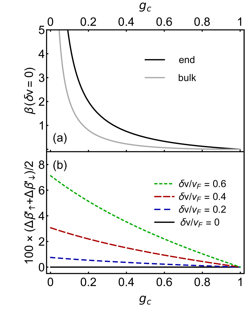
Figure 7: (a) Exponents of the density of states as a function of the interaction parameter ($g_{c}$) for $g_{s}=1$ and $\delta v=0$. The black (gray) curve corresponds to the boundary (bulk) exponent $\beta_{\sigma}^{\prime}$ ($\beta_{\sigma}^{\prime~{}{\rm bulk}}$) given in Eq. (76) [Eq. (75)]. Since we are plotting the zero-spin-orbit value, these curves are identical to those given in Eqs. (56) and (63) and do not depend on the species $r$ or $\sigma$. We therefore neglect the superscript and the subscript. (b) Interaction parameter ($g_{c}$) dependence of the change of the boundary exponent (multiplied by 100 for clarity) with respect to its zero-spin-orbit value for $g_{s}=1$ and several values of $\delta v/v_{F}$. The curves correspond to the boundary exponent $\beta_{\sigma}^{\prime}$ given in Eq. (76), upon taking average over $\sigma=1$ and $\sigma=-1$.

Diagonalizing the Hamiltonian $H^{\prime}$, we get

$$H^{\prime} = \sum_{\nu}\int\frac{\hbar dx}{2\pi}\left[u_{\nu}^{\prime\prime}g_{\nu}^{\prime\prime}\left(\partial_{x}\theta_{\nu}^{\prime\prime}\right)^{2}+\frac{u_{\nu}^{\prime\prime}}{g_{\nu}^{\prime\prime}}\left(\partial_{x}\phi_{\nu}^{\prime\prime}\right)^{2}\right],$$ (71)

where the new fields are

$$\left(\begin{array}[]{c}\phi_{c}^{\prime\prime}\\ \phi_{s}^{\prime\prime}\end{array}\right) = \left(\begin{array}[]{cc}\cos\theta^{\prime}&g_{0}^{\prime}\sin\theta^{\prime}\\ -\frac{1}{g_{0}^{\prime}}\sin\theta^{\prime}&\cos\theta^{\prime}\end{array}\right)\left(\begin{array}[]{c}\phi_{c}\\ \phi_{s}\end{array}\right),$$ (72g)

$$\left(\begin{array}[]{c}\theta_{c}^{\prime\prime}\\ \theta_{s}^{\prime\prime}\end{array}\right) = \left(\begin{array}[]{cc}\cos\theta^{\prime}&\frac{1}{g_{0}^{\prime}}\sin\theta^{\prime}\\ -g_{0}^{\prime}\sin\theta^{\prime}&\cos\theta^{\prime}\end{array}\right)\left(\begin{array}[]{c}\theta_{c}\\ \theta_{s}\end{array}\right),$$ (72n)

with the parameters

$$g_{0}^{\prime} = \frac{g_{c}}{g_{s}}\sqrt{\frac{1+g_{s}^{2}}{1+g_{c}^{2}}},$$ (73a)

$$\theta^{\prime} = \frac{1}{2}\arctan\left(\frac{\delta v}{v_{F}}\frac{g_{c}g_{s}\sqrt{(1+g_{s}^{2})(1+g_{c}^{2})}}{g_{s}^{2}-g_{c}^{2}}\right).$$ (73b)

The modified interaction parameters and velocities are related to the original parameters through

$$\frac{u_{c}^{\prime\prime}}{g_{c}^{\prime\prime}}=\frac{u_{c}}{g_{c}}\cos^{2}\theta^{\prime}+\frac{u_{s}}{g_{s}(g_{0}^{\prime})^{2}}\sin^{2}\theta^{\prime}+\frac{\delta v}{2g_{0}^{\prime}}\sin(2\theta^{\prime}),$$ (74a)

$$\frac{u_{s}^{\prime\prime}}{g_{s}^{\prime\prime}}=\frac{u_{s}}{g_{s}}\cos^{2}\theta^{\prime}+\frac{u_{c}(g_{0}^{\prime})^{2}}{g_{c}}\sin^{2}\theta^{\prime}-\frac{\delta vg_{0}^{\prime}}{2}\sin(2\theta^{\prime}),$$ (74b)

$$u_{c}^{\prime\prime}g_{c}^{\prime\prime}=u_{c}g_{c}\cos^{2}\theta^{\prime}+u_{s}g_{s}(g_{0}^{\prime})^{2}\sin^{2}\theta^{\prime}+\frac{\delta vg_{0}^{\prime}}{2}\sin(2\theta^{\prime}),$$ (74c)

$$u_{s}^{\prime\prime}g_{s}^{\prime\prime}=u_{s}g_{s}\cos^{2}\theta^{\prime}+\frac{u_{c}g_{c}}{(g_{0}^{\prime})^{2}}\sin^{2}\theta^{\prime}-\frac{\delta v}{2g_{0}^{\prime}}\sin(2\theta^{\prime}).$$ (74d)

Following the same procedure as in Appendix A, we compute the density of states in the bulk and at the end of the wire. For a given $\sigma$, the former is given by $\rho_{\sigma}^{\rm bulk}(\epsilon)\propto\epsilon^{\beta_{\sigma}^{\prime{\rm bulk}}}$ with the exponent,

$$\beta_{\sigma}^{\prime{\rm bulk}}=\frac{g_{c}^{\prime\prime}}{4}\left(\cos\theta^{\prime}+\frac{\sigma}{g_{0}^{\prime}}\sin\theta^{\prime}\right)^{2}+\frac{\left(\cos\theta^{\prime}+\sigma g_{0}^{\prime}\sin\theta^{\prime}\right)^{2}}{4g_{c}^{\prime\prime}}$$

$$+\frac{g_{s}^{\prime\prime}}{4}\left(\cos\theta^{\prime}-\sigma g_{0}^{\prime}\sin\theta^{\prime}\right)^{2}+\frac{\left(\cos\theta^{\prime}-\frac{\sigma}{g_{0}^{\prime}}\sin\theta^{\prime}\right)^{2}}{4g_{s}^{\prime\prime}}-1.$$ (75)

On the other hand, at the end of the wire, the density of states becomes $\rho_{\sigma}^{\rm end}(\epsilon)\propto\epsilon^{\beta_{\sigma}^{\prime}}$ with

$$\beta_{\sigma}^{\prime}=\frac{\left(\cos\theta^{\prime}+\sigma g_{0}^{\prime}\sin\theta^{\prime}\right)^{2}}{2g_{c}^{\prime\prime}}+\frac{\left(\cos\theta^{\prime}-\frac{\sigma}{g_{0}^{\prime}}\sin\theta^{\prime}\right)^{2}}{2g_{s}^{\prime\prime}}-1.$$ (76)

The exponents in Eqs. (75)–(76) are analogous to Eqs. (56) and (63) of the bosonized model introduced in Refs. Moroz et al. (2000a, b). The exponents can be extracted through the density of states measurement using scanning tunneling spectroscopy. Their behavior is displayed in Fig. 7. Similar to the standard Luttinger liquid Kane and Fisher (1992b); Balents (1999), the suppression of the density of states is stronger at the end than in the bulk of the wire. In contrast to the strong dependence on the position of the probe [see Fig. 7(a)], the spin-orbit-induced change is negligible [see Fig. 7(b)].

Appendix D An alternative approach for the weak-impurity analysis 

Here we discuss an alternative approach for the analysis in the weak-impurity regime. In Sec. III.2 we start our analysis by treating a weak impurity as an isolated object (referred to as weak barrier in Ref. Kane and Fisher (1992b)), such that it creates a potential which is nonzero only near $x=0$ with the strength $V_{0}$. Following Ref. Kane and Fisher (1992b) to construct the RG flow equation for $\tilde{V}_{0}$, we obtain the exponent $\alpha_{\rm imp}$ of the conductance correction due to a single impurity. Then, as discussed in Ref. Giamarchi (2003), assuming that the contributions from multiple impurities are additive, many weak impurities lead to a power-law conductance characterized by the parameter $\alpha_{\rm imp}$.

Alternatively, one can start with random backscattering potential generated by impurities which are not isolated, as in Ref. Giamarchi (2003). In that reference, such disorder is named “extended disorder” or “uniform disorder” and assumed to be of Gaussian type. Then, one can apply the replica method to average over the disorder and then perform the RG analysis. In this case, there would be additional RG flow equations for the interaction parameters $g_{c}$ and $g_{s}$ and velocities, depending on the disorder strength. The additional RG flow equations arise because in this case impurities can affect bulk quantities, in contrast to isolated impurities, which cannot. Importantly for us, the renormalization of $g_{c}$, $g_{s}$ due to weak disorder is typically negligible, which would lead to the same power-law conductance in the high-$T$ or high-$V$ regimes as in the isolated-impurities scenario. As a result, there would be no significant difference for the power-law conductance, which is the main focus of this work. We note that, if other phenomena such as localization are concerned, the “extended disorder” scenario would better describe the physical picture, as discussed in Ref. Giamarchi (2003). Nevertheless, to give a better connection between the strong- and weak-impurity cases, we adopt the isolated-impurity picture for our discussion throughout the article.

References

- Tomonaga (1950) S. Tomonaga, Remarks on Bloch’s Method of Sound Waves applied to Many-Fermion Problems, Prog. Theor. Phys. 5, 544 (1950).
- Luttinger (1963) J. M. Luttinger, An Exactly Soluble Model of a Many-Fermion System, J. Math. Phys. 4, 1154 (1963).
- Haldane (1981) F. D. M. Haldane, Luttinger liquid theory of one-dimensional quantum fluids. I. Properties of the Luttinger model and their extension to the general 1D interacting spinless Fermi gas, J. Phys. C: Solid State Physics 14, 2585 (1981).
- Voit (1995) J. Voit, One-dimensional Fermi liquids, Rep. Prog. Phys. 58, 977 (1995).
- von Delft and Schoeller (1998) J. von Delft and H. Schoeller, Bosonization for beginners–refermionization for experts, Ann. Phys. 7, 225 (1998).
- Giamarchi (2003) T. Giamarchi, Quantum Physics in One Dimension (Oxford University Press, New York, 2003).
- Maslov and Stone (1995) D. L. Maslov and M. Stone, Landauer conductance of Luttinger liquids with leads, Phys. Rev. B 52, R5539 (1995).
- Ponomarenko (1995) V. V. Ponomarenko, Renormalization of the one-dimensional conductance in the Luttinger-liquid model, Phys. Rev. B 52, R8666 (1995).
- Safi and Schulz (1995) I. Safi and H. J. Schulz, Transport in an inhomogeneous interacting one-dimensional system, Phys. Rev. B 52, R17040 (1995).
- Kane and Fisher (1992a) C. L. Kane and M. P. A. Fisher, Transport in a one-channel Luttinger liquid, Phys. Rev. Lett. 68, 1220 (1992a).
- Kane and Fisher (1992b) C. L. Kane and M. P. A. Fisher, Transmission through barriers and resonant tunneling in an interacting one-dimensional electron gas, Phys. Rev. B 46, 15233 (1992b).
- Furusaki and Nagaosa (1993) A. Furusaki and N. Nagaosa, Single-barrier problem and Anderson localization in a one-dimensional interacting electron system, Phys. Rev. B 47, 4631 (1993).
- Matveev and Glazman (1993) K. A. Matveev and L. I. Glazman, Coulomb blockade of tunneling into a quasi-one-dimensional wire, Phys. Rev. Lett. 70, 990 (1993).
- Maslov (1995) D. L. Maslov, Transport through dirty Luttinger liquids connected to reservoirs, Phys. Rev. B 52, R14368 (1995).
- Sandler and Maslov (1997) N. P. Sandler and D. L. Maslov, Interactions and disorder in multichannel quantum wires, Phys. Rev. B 55, 13808 (1997).
- Balents (1999) L. Balents, Orthogonality Catastrophes in Carbon Nanotubes, eprint arXiv:cond-mat/9906032 (1999), cond-mat/9906032 .
- Tarucha et al. (1995) S. Tarucha, T. Honda, and T. Saku, Reduction of quantized conductance at low temperatures observed in 2 to 10 m-long quantum wires, Solid State Commun. 94, 413 (1995).
- Datta and Das (1990) S. Datta and B. Das, Electronic analog of the electro-optic modulator, Appl. Phys. Lett. 56, 665 (1990).
- Nitta et al. (1997) J. Nitta, T. Akazaki, H. Takayanagi, and T. Enoki, Gate Control of Spin-Orbit Interaction in an Inverted IGAs/IAAs Heterostructure, Phys. Rev. Lett. 78, 1335 (1997).
- Fasth et al. (2007) C. Fasth, A. Fuhrer, L. Samuelson, V. N. Golovach, and D. Loss, Direct Measurement of the Spin-Orbit Interaction in a Two-Electron InAs Nanowire Quantum Dot, Phys. Rev. Lett. 98, 266801 (2007).
- Fabian et al. (2007) J. Fabian, A. Matos-Abiague, C. Ertler, P. Stano, and I. Žutić, Semiconductor spintronics, Acta Phys. Slovaca 57, 565 (2007).
- Nadj-Perge et al. (2010) S. Nadj-Perge, S. M. Frolov, E. P. A. M. Bakkers, and L. P. Kouwenhoven, Spin-orbit qubit in a semiconductor nanowire, Nature 468, 1084 (2010).
- Lutchyn et al. (2010) R. M. Lutchyn, J. D. Sau, and S. Das Sarma, Majorana Fermions and a Topological Phase Transition in Semiconductor-Superconductor Heterostructures, Phys. Rev. Lett. 105, 077001 (2010).
- Oreg et al. (2010) Y. Oreg, G. Refael, and F. von Oppen, Helical Liquids and Majorana Bound States in Quantum Wires, Phys. Rev. Lett. 105, 177002 (2010).
- Mourik et al. (2012) V. Mourik, K. Zuo, S. M. Frolov, S. R. Plissard, E. P. A. M. Bakkers, and L. P. Kouwenhoven, Signatures of Majorana Fermions in Hybrid Superconductor-Semiconductor Nanowire Devices, Science 336, 1003 (2012).
- Das et al. (2012) A. Das, Y. Ronen, Y. Most, Y. Oreg, M. Heiblum, and H. Shtrikman, Zero-bias peaks and splitting in an InAs nanowire topological superconductor as a signature of Majorana fermions, Nat. Phys. 8, 887 (2012).
- Deng et al. (2012) M. T. Deng, C. L. Yu, G. Y. Huang, M. Larsson, P. Caroff, and H. Q. Xu, Anomalous Zero-Bias Conductance Peak in a Nb–InSb Nanowire–Nb Hybrid Device, Nano Lett. 12, 6414 (2012).
- Rokhinson et al. (2012) L. P. Rokhinson, X. Liu, and J. K. Furdyna, The fractional a.c. Josephson effect in a semiconductor–superconductor nanowire as a signature of Majorana particles, Nat. Phys. 8, 795 (2012).
- Churchill et al. (2013) H. O. H. Churchill, V. Fatemi, K. Grove-Rasmussen, M. T. Deng, P. Caroff, H. Q. Xu, and C. M. Marcus, Superconductor-nanowire devices from tunneling to the multichannel regime: Zero-bias oscillations and magnetoconductance crossover, Phys. Rev. B 87, 241401(R) (2013).
- Gaidamauskas et al. (2014) E. Gaidamauskas, J. Paaske, and K. Flensberg, Majorana Bound States in Two-Channel Time-Reversal-Symmetric Nanowire Systems, Phys. Rev. Lett. 112, 126402 (2014).
- Ebisu et al. (2016) H. Ebisu, B. Lu, J. Klinovaja, and Y. Tanaka, Theory of time-reversal topological superconductivity in double Rashba wires: symmetries of Cooper pairs and Andreev bound states, Prog. Theo. Exp. Phys. 2016, 083I01 (2016).
- Reeg et al. (2017) C. Reeg, J. Klinovaja, and D. Loss, Destructive interference of direct and crossed Andreev pairing in a system of two nanowires coupled via an -wave superconductor, Phys. Rev. B 96, 081301(R) (2017).
- Schrade et al. (2017) C. Schrade, M. Thakurathi, C. Reeg, S. Hoffman, J. Klinovaja, and D. Loss, Low-field topological threshold in Majorana double nanowires, Phys. Rev. B 96, 035306 (2017).
- Thakurathi et al. (2018) M. Thakurathi, P. Simon, I. Mandal, J. Klinovaja, and D. Loss, Majorana Kramers pairs in Rashba double nanowires with interactions and disorder, Phys. Rev. B 97, 045415 (2018).
- Klinovaja and Loss (2014a) J. Klinovaja and D. Loss, Parafermions in an Interacting Nanowire Bundle, Phys. Rev. Lett. 112, 246403 (2014a).
- Klinovaja and Loss (2014b) J. Klinovaja and D. Loss, Time-reversal invariant parafermions in interacting Rashba nanowires, Phys. Rev. B 90, 045118 (2014b).
- Oreg et al. (2014) Y. Oreg, E. Sela, and A. Stern, Fractional helical liquids in quantum wires, Phys. Rev. B 89, 115402 (2014).
- Alicea and Fendley (2016) J. Alicea and P. Fendley, Topological Phases with Parafermions: Theory and Blueprints, Ann. Rev. Condens. Matter Phys. 7, 119 (2016).
- Ueda et al. (2019) K. Ueda, S. Matsuo, H. Kamata, S. Baba, Y. Sato, Y. Takeshige, K. Li, S. Jeppesen, L. Samuelson, H. Xu, and S. Tarucha, Dominant nonlocal superconducting proximity effect due to electron-electron interaction in a ballistic double nanowire, Sci. Adv. 5, eaaw2194 (2019).
- Sato et al. (2019) Y. Sato, S. Matsuo, C.-H. Hsu, P. Stano, K. Ueda, Y. Takeshige, H. Kamata, J. S. Lee, B. Shojaei, K. Wickramasinghe, J. Shabani, C. Palmstrøm, Y. Tokura, D. Loss, and S. Tarucha, Strong electron-electron interactions of a Tomonaga-Luttinger liquid observed in InAs quantum wires, Phys. Rev. B 99, 155304 (2019).
- Bockrath et al. (1999) M. Bockrath, D. H. Cobden, J. Lu, A. G. Rinzler, R. E. Smalley, L. Balents, and P. L. McEuen, Luttinger-liquid behaviour in carbon nanotubes, Nature 397, 598 (1999).
- Luo et al. (1988) J. Luo, H. Munekata, F. F. Fang, and P. J. Stiles, Observation of the zero-field spin splitting of the ground electron subband in GaSb/InAs/GaSb quantum wells, Phys. Rev. B 38, 10142 (1988).
- Luo et al. (1990) J. Luo, H. Munekata, F. F. Fang, and P. J. Stiles, Effects of inversion asymmetry on electron energy band structures in GaSb/InAs/GaSb quantum wells, Phys. Rev. B 41, 7685 (1990).
- Grundler (2000) D. Grundler, Large Rashba Splitting in InAs Quantum Wells due to Electron Wave Function Penetration into the Barrier Layers, Phys. Rev. Lett. 84, 6074 (2000).
- Heedt et al. (2017) S. Heedt, N. Traverso Ziani, F. Crépin, W. Prost, St. Trellenkamp, J. Schubert, D. Grützmacher, B. Trauzettel, and Th. Schäpers, Signatures of interaction-induced helical gaps in nanowire quantum point contacts, Nat. Phys. 13, 563 (2017).
- Braunecker et al. (2010) B. Braunecker, G. I. Japaridze, J. Klinovaja, and D. Loss, Spin-selective Peierls transition in interacting one-dimensional conductors with spin-orbit interaction, Phys. Rev. B 82, 045127 (2010).
- Meng et al. (2014) T. Meng, J. Klinovaja, and D. Loss, Renormalization of anticrossings in interacting quantum wires with Rashba and Dresselhaus spin-orbit couplings, Phys. Rev. B 89, 205133 (2014).
- Kainaris and Carr (2015) N. Kainaris and S. T. Carr, Emergent topological properties in interacting one-dimensional systems with spin-orbit coupling, Phys. Rev. B 92, 035139 (2015).
- Moroz and Barnes (1999) A. V. Moroz and C. H. W. Barnes, Effect of the spin-orbit interaction on the band structure and conductance of quasi-one-dimensional systems, Phys. Rev. B 60, 14272 (1999).
- Governale and Zülicke (2002) M. Governale and U. Zülicke, Spin accumulation in quantum wires with strong Rashba spin-orbit coupling, Phys. Rev. B 66, 073311 (2002).
- Moroz et al. (2000a) A. V. Moroz, K. V. Samokhin, and C. H. W. Barnes, Spin-Orbit Coupling in Interacting Quasi-One-Dimensional Electron Systems, Phys. Rev. Lett. 84, 4164 (2000a).
- Moroz et al. (2000b) A. V. Moroz, K. V. Samokhin, and C. H. W. Barnes, Theory of quasi-one-dimensional electron liquids with spin-orbit coupling, Phys. Rev. B 62, 16900 (2000b).
- Gritsev et al. (2005) V. Gritsev, G. I. Japaridze, M. Pletyukhov, and D. Baeriswyl, Competing Effects of Interactions and Spin-Orbit Coupling in a Quantum Wire, Phys. Rev. Lett. 94, 137207 (2005).
- Schulz et al. (2009) A. Schulz, A. De Martino, P. Ingenhoven, and R. Egger, Low-energy theory and RKKY interaction for interacting quantum wires with Rashba spin-orbit coupling, Phys. Rev. B 79, 205432 (2009).
- Sun et al. (2007) J. Sun, S. Gangadharaiah, and O. A. Starykh, Spin-Orbit-Induced Spin-Density Wave in a Quantum Wire, Phys. Rev. Lett. 98, 126408 (2007).
- Gangadharaiah et al. (2008) S. Gangadharaiah, J. Sun, and O. A. Starykh, Spin-orbital effects in magnetized quantum wires and spin chains, Phys. Rev. B 78, 054436 (2008).
- Schmidt (2013) T. L. Schmidt, Finite-temperature conductance of interacting quantum wires with Rashba spin-orbit coupling, Phys. Rev. B 88, 235429 (2013).
- Tretiakov et al. (2013) O. A. Tretiakov, K. S. Tikhonov, and V. L. Pokrovsky, Spin resonance in a Luttinger liquid with spin-orbit interaction, Phys. Rev. B 88, 125143 (2013).
- Pedder et al. (2016) C. J. Pedder, T. Meng, R. P. Tiwari, and T. L. Schmidt, Dynamic response functions and helical gaps in interacting Rashba nanowires with and without magnetic fields, Phys. Rev. B 94, 245414 (2016).
- Pedder et al. (2017) C. J. Pedder, T. Meng, R. P. Tiwari, and T. L. Schmidt, Missing Shapiro steps and the -periodic Josephson effect in interacting helical electron systems, Phys. Rev. B 96, 165429 (2017).
- Iucci (2003) A. Iucci, Correlation functions for one-dimensional interacting fermions with spin-orbit coupling, Phys. Rev. B 68, 075107 (2003).
- Governale and Zülicke (2004) M. Governale and U. Zülicke, Rashba spin splitting in quantum wires, Solid State Commun. 131, 581 (2004).
- Rainis and Loss (2014) D. Rainis and D. Loss, Conductance behavior in nanowires with spin-orbit interaction: A numerical study, Phys. Rev. B 90, 235415 (2014).
- Hsu et al. (2017) C.-H. Hsu, P. Stano, J. Klinovaja, and D. Loss, Nuclear-spin-induced localization of edge states in two-dimensional topological insulators, Phys. Rev. B 96, 081405(R) (2017).
- Hsu et al. (2018) C.-H. Hsu, P. Stano, J. Klinovaja, and D. Loss, Effects of nuclear spins on the transport properties of the edge of two-dimensional topological insulators, Phys. Rev. B 97, 125432 (2018).
- Egger and Grabert (1998) R. Egger and H. Grabert, Applying voltage sources to a Luttinger liquid with arbitrary transmission, Phys. Rev. B 58, 10761 (1998).
- Aseev et al. (2018) P. P. Aseev, D. Loss, and J. Klinovaja, Conductance of fractional Luttinger liquids at finite temperatures, Phys. Rev. B 98, 045416 (2018).
- Meden et al. (2003) V. Meden, S. Andergassen, W. Metzner, U. Schollwöck, and K. Schönhammer, Scaling of the conductance in a quantum wire, Europhys. Lett. 64, 769 (2003).
- Janzen et al. (2006) K. Janzen, V. Meden, and K. Schönhammer, Influence of the contacts on the conductance of interacting quantum wires, Phys. Rev. B 74, 085301 (2006).
- Schrieffer et al. (1963) J. R. Schrieffer, D. J. Scalapino, and J. W. Wilkins, Effective Tunneling Density of States in Superconductors, Phys. Rev. Lett. 10, 336 (1963).
- Wen (1991) X.-G. Wen, Edge transport properties of the fractional quantum Hall states and weak-impurity scattering of a one-dimensional charge-density wave, Phys. Rev. B 44, 5708 (1991).
- Jakobs et al. (2007) S. G. Jakobs, V. Meden, H. Schoeller, and T. Enss, Temperature-induced phase averaging in one-dimensional mesoscopic systems, Phys. Rev. B 75, 035126 (2007).
- Väyrynen et al. (2016) J. I. Väyrynen, F. Geissler, and L. I. Glazman, Magnetic moments in a helical edge can make weak correlations seem strong, Phys. Rev. B 93, 241301(R) (2016).
- Stühler et al. (2019) R. Stühler, F. Reis, T. Müller, T. Helbig, T. Schwemmer, R. Thomale, J. Schäfer, and R. Claessen, Tomonaga-Luttinger liquid in the edge channels of a quantum spin Hall insulator, Nat. Phys. (2019), 10.1038/s41567-019-0697-z.
- Maciejko et al. (2009) J. Maciejko, C. Liu, Y. Oreg, X.-L. Qi, C. Wu, and S.-C. Zhang, Kondo Effect in the Helical Edge Liquid of the Quantum Spin Hall State, Phys. Rev. Lett. 102, 256803 (2009).
- Gradshteyn and Ryzhik (1980) I. Gradshteyn and I. Ryzhik, Table of Integrals, Series, and Products (Academic Press, New York, 1980).