Is Symmetry Breaking into Special Subgroup Special?

Abstract

The purpose of this paper is to show that the symmetry breaking into special subgroups is not special at all, contrary to the usual wisdom. To demonstrate this explicitly, we examine dynamical symmetry breaking pattern in 4D $SU(N)$ Nambu–Jona-Lasinio type models in which the fermion matter belongs to an irreducible representation of $SU(N)$. The potential analysis shows that for almost all cases at the potential minimum the $SU(N)$ group symmetry is broken to its special subgroups such as $SO(N)$ or $USp(N)$ when symmetry breaking occurs.

1 Introduction

Symmetries and their breaking[1, 2, 3] are important to consider not only the Standard Model (SM) but also unified theories beyond the SM in particle physics. In the framework of quantum field theories (QFTs), several symmetry breaking mechanisms have been already known, e.g., the Higgs mechanism[4, 5, 6], and the dynamical symmetry breaking mechanism[1, 2, 7, 8, 9, 10, 11, 12, 13, 14, 15, 16, 17, 18]; in higher dimensional and string-inspired theories, the Hosotani mechanism[19, 20, 21], magnetic flux [22, 23] and orbifold breaking mechanism[24, 25].

For $SU(n)$ and its breaking via the Higgs mechanism[26], it is well-known that $SU(n)$ symmetry is broken to $SU(n-1)$ and $SU(m)\times SU(n-m)\times U(1)$ by the non-vanishing vacuum expectation value (VEV) of a scalar field in an $SU(n)$ fundamental representation ${\bf n}$ and an $SU(n)$ adjoint representation ${\bf n^{2}-1}$, respectively. On the other hand, $SU(n)$ symmetry is broken to $SU(n-1)$ or $SO(n)$ and $SU(n-2)$ or $USp(2\ell)(\ell:=[n/2])$ by the non-vanishing VEV of a scalar field in an $SU(n)$ 2nd-rank symmetric tensor representation ${\bf n(n+1)/2}$ and an $SU(n)$ 2nd-rank anti-symmetric tensor representation ${\bf n(n-1)/2}$, respectively.

The above subgroups $SU(n-1)$, $SU(m)\times SU(n-m)\times U(1)$, $SU(n-1)$, and $SU(n-2)$ are regular subgroups of $SU(n)$, while the $SO(n)$ and $USp(2\ell)$ are special subgroups (or irregular subgroups) of $SU(n)$ [27, 28]. Note that a subgroup $H$ of a group $G$ is called a regular subgroup if all the Cartan subgroups of $H$ are also the Cartan subgroups of $G$; otherwise, the subgroup $H$ is called a special subgroup. For example, $SU(2)\times U(1)$ of $SU(3)$ is a regular subgroup, while $SO(3)\simeq SU(2)$ of $SU(3)$ is a special subgroup. If we use the familiar Gell-Mann matrices $\lambda^{a}$ ($a=1-8)$ for the $SU(3)$ generators, the regular subgroup $SU(2)\times U(1)$ has the generators $\lambda_{1},\lambda_{2},\lambda_{3},\lambda_{8}$ when the $SU(2)$ is the usual isospin subgroup, while the generators of the special subgroup $SO(3)$ are the three anti-symmetric (hence, purely imaginary) matrices $\lambda_{2},\lambda_{5},\lambda_{7}$. Note that all regular subgroups are obtained by deleting circles from (extended) Dynkin diagrams, while all special subgroups are not done so. (For review, see e.g., Refs. [29, 30, 31].)

For grand unified theories (GUTs) in 4 dimensional (4D) theories [32, 33, 34, 35, 36, 37, 30, 38, 31] and higher dimensional theories [39, 40, 41, 42, 43, 44, 45, 46, 47, 48, 49, 50, 51, 52, 53], a lot of GUT models use the Lie groups and their regular subgroups in a series:

$$E_{6}\supset SO(10)\supset SU(5)\supset G_{\rm SM},$$ (1.1)

where $G_{\rm SM}:=SU(3)_{C}\times SU(2)_{L}\times U(1)_{Y}$, and we omitted several $U(1)$ subgroups. A few GUT models [54, 55, 56] are known to use not only the regular subgroups but also special subgroups such as

$$SO(32)\supset SU(16)\supset SO(10)\supset SU(5)\supset G_{\rm SM},$$ (1.2)

where we omitted several $U(1)$ subgroups for regular subgroups. The $SU(16)$ group has a maximal special subgroup $SO(10)$, 16 spinor of which is identified with the defining 16 representation of $SU(16)$. The $SU(16)$ symmetry can be broken to $SO(10)$ via the VEV of the $SU(16)$ ${\bf 5440}$ representation corresponding to a Young tableau                                  . Note that a subgroup $H$ of $G$ is called maximal if there is no larger subgroup containing it except $G$ itself. For example, $U(1)\times U(1)$ of $SU(3)$ is not a maximal subgroup because one of $U(1)$ is contained in the regular subgroup $SU(2)\subset SU(3)$. Some typical examples of the maximal special subgroups of $SU(n)$ are listed in Table 1.

Rank	$G\supset H$	Condition
$mn-1$	$SU(mn)\supset SU(m)\times SU(n)$	$(m,n\geq 2)$
$2n$	$SU(2n+1)\supset SO(2n+1)$	$(n\geq 1)$
$2n-1$	$SU(2n)\supset USp(2n),SO(2n)$	$(n\geq 2)$
$\frac{(n+1)(n-2)}{2}$	$SU\left({\frac{(n(n-1)}{2}}\right)\supset SU(n)$	$(n\geq 3)$
$\frac{(n-1)(n+2)}{2}$	$SU\left({\frac{n(n+1)}{2}}\right)\supset SU(n)$	$(n\geq 2)$
$15$	$SU(16)\supset SO(10)$
$26$	$SU(27)\supset E_{6}$

Table 1: $H$ is a maximal special subgroup of $G=SU(N)$. This table is a part of Tables 4 and 5 of Ref. [31]. Note that this table is not a complete list of maximal special subgroups.

When we discuss spontaneous symmetry breaking, it is important to know not only subgroups but also little groups. A little group $H_{\phi}$ of a vector $\phi$ in a representation ${\boldsymbol{R}}$ of $G$ is defined by

$$H_{\phi}:=\Bigl{\{}g\ \Big{|}\ g\phi=\phi,\ g\in G\ \Bigr{\}}.$$ (1.3)

This little group $H_{\phi}$ of $G$ depends not only on the representation ${\boldsymbol{R}}$ of $\phi$ but also the vector (value) $\phi$ itself. The vector $\phi$ must be an $H_{\phi}$-singlet, so that a subgroup $H$ can be a little group of $G$ for some representation ${\boldsymbol{R}}$ only when ${\boldsymbol{R}}$ contains at least one $H$-singlet. For example, the maximal little groups of $SU(3)$ ${\bf 3}$, ${\bf 6}$, and ${\bf 8}$ representations are $SU(2)$(R), $SU(2)$(R) and $SO(3)$(S), and $SU(2)\times U(1)$(R), where (R) and (S) stand for regular and special subgroups, respectively. Practically, the so-called Michel’s conjecture [57] are very useful. The Michel’s conjecture tells us that a potential that consists of a scalar field in an irreducible representation ${\boldsymbol{R}}$ of a group $G$ has its potential minimum that preserves one of its maximal little groups $H$ of ${\boldsymbol{R}}$. This conjecture drastically reduces the number of states especially for higher rank group cases.

Many people vaguely believe that symmetry groups are broken to only regular subgroups, not to special subgroups. The main purpose of this paper is to show that symmetry breaking into special subgroups are not special by using 4D Nambu–Jona-Lasinio (NJL) type model in the framework of dynamical symmetry breaking scenario [58].

This paper is organized as follows. In Sec. 2 we first review a 4D NJL type model to show the method of potential analysis. In Secs. 3 and 4, we apply the method for two cases in which the fermion belongs to the defining representation and rank-2 anti-symmetric representations of $SU(n)$, respectively. For the latter NJL model with rank-2 anti-symmetric fermion, we will show, in particular, that $SU(16)$ symmetry breaks into two degenerate vacua of special subgroups $SO(16)$ and $SO(10)$ for a certain region of coupling constants. However, this degeneracy actually turns out to cause the mixing of the two vacua and leads to the total breaking of the $SU(16)$ symmetry, generally. Some detailed identification of the scalar VEVs is necessary to discuss this mixing phenomenon of the degenerate vacua, so the task will be given in the Appendix. Section 5 is devoted to a summary and discussions, where we also note the similarity of the present results to the previous one in Ref. [58] for the $E_{6}$ NJL model with fundamental 27 fermion.

2 Nambu–Jona-Lasinio type model

We consider a 4D Nambu-Jona-Lasinio (NJL) type model [1, 2] in which the fermion matter $\psi=(\psi_{I})$ ($I=1,2,\cdots,{\rm dim}{\boldsymbol{R}}=d$) belongs to an irreducible representation ${\boldsymbol{R}}$ of dimension $d$ of the group $G$. The each fermion field $\psi_{I}$ is the two-component left-handed spinor $\psi_{I\alpha}$ with an undotted spinor index $\alpha$ running over 1 to 2. Then the Lorentz scalar fermion bilinears $\psi_{I}\psi_{J}:=\psi_{I}^{\alpha}\psi_{J\alpha}:=\varepsilon^{\alpha\beta}\psi_{I\beta}\psi_{J\alpha}$ and $\bar{\psi}^{I}\bar{\psi}^{J}:=\bar{\psi}^{I}_{\dot{\alpha}}\bar{\psi}^{J\dot{\alpha}}=(\psi_{I}\psi_{J})^{*}$ are symmetric under exchange $I\leftrightarrow J$ owing to the Fermi statistics of $\psi_{I}$. Assume that the symmetric tensor product $({\boldsymbol{R}}\times{\boldsymbol{R}})_{\rm S}$ is decomposed into $n_{R}$ irreducible representations ${\boldsymbol{R}}_{p}$:

$$({\boldsymbol{R}}\times{\boldsymbol{R}})_{\rm S}=\sum_{p=1}^{n_{R}}\,{\boldsymbol{R}}_{p}.$$ (2.1)

Then the NJL Lagrangian has $n_{R}$ independent 4-fermion interaction terms:

$${\cal L}= \bar{\psi}^{I}\,i\overline{\sigma}^{\mu}\partial_{\mu}\psi_{I}+\sum_{p=1}^{n_{R}}\frac{1}{4}{G_{{\boldsymbol{R}}_{p}}}\bigl{(}\psi_{I}\psi_{J}\bigr{)}_{{\boldsymbol{R}}_{p}}\bigl{(}\bar{\psi}^{I}\bar{\psi}^{J}\bigr{)}_{\overline{\boldsymbol{R}}_{p}},$$ (2.2)

where $\bigl{(}\psi_{I}\psi_{J}\bigr{)}_{{\boldsymbol{R}}_{p}}$ denotes the projection of the fermion bilinear into the irreducible component ${\boldsymbol{R}}_{p}$. Introducing auxiliary complex scalar fields $\Phi_{{\boldsymbol{R}}_{p}}$ ($p=1,\cdots,n_{R}$) standing for each of the irreducible components $-(G_{{\boldsymbol{R}}_{p}}/2)\bigl{(}\psi_{I}\psi_{J}\bigr{)}_{{\boldsymbol{R}}_{p}}$ [59, 60], we rewrite this Lagrangian into

$${\cal L} =\bar{\psi}^{I}i\bar{{\ooalign{\hfil/\hfil\crcr$\partial$}}}\psi_{I}-\sum_{p=1}^{n_{R}}\left\{\frac{1}{2}\bigl{(}\psi_{I}\psi_{J}\bigr{)}_{{\boldsymbol{R}}_{p}}\Phi_{{\boldsymbol{R}}_{p}}^{{\dagger}IJ}+\frac{1}{2}\bigl{(}\bar{\psi}^{I}\bar{\psi}^{J}\bigr{)}_{\overline{\boldsymbol{R}}_{p}}\Phi_{{\boldsymbol{R}}_{p}IJ}+M^{2}_{{\boldsymbol{R}}_{p}}\,\Phi_{{\boldsymbol{R}}_{p}}^{{\dagger}\,IJ}\!\Phi_{{\boldsymbol{R}}_{p}\,IJ}\right\}$$ (2.5)

$$=\bar{\psi}^{I}i\bar{{\ooalign{\hfil/\hfil\crcr$\partial$}}}\psi_{I}-\frac{1}{2}\psi_{I}\psi_{J}\Phi^{{\dagger}\,IJ}-\frac{1}{2}\bar{\psi}^{I}\bar{\psi}^{J}\Phi_{IJ}-\sum_{p=1}^{n_{R}}M^{2}_{{\boldsymbol{R}}_{p}}\,\mathop{\text{tr}}\bigl{(}\Phi_{{\boldsymbol{R}}_{p}}^{{\dagger}}\Phi_{{\boldsymbol{R}}_{p}}\bigr{)},$$ (2.8)

where $\bar{{\ooalign{\hfil/\hfil\crcr$\partial$}}}:=\bar{\sigma}^{\mu}\partial_{\mu}$, $M^{2}_{{\boldsymbol{R}}_{p}}:=1/G_{{\boldsymbol{R}}_{p}}$, $\Phi_{IJ}$ without irreducible index ${\boldsymbol{R}}_{p}$ was introduced in the second line to denote the sum

$$\Phi_{IJ}=\sum_{p=1}^{n_{R}}\Phi_{{\boldsymbol{R}}_{p}IJ},$$ (2.9)

which now stands for the general symmetric $d\times d$ complex matrix with no more constraint. Now, noting that the kinetic and Yukawa terms of the fermion can be rewritten into

$$\bar{\psi}^{I}i\bar{{\ooalign{\hfil/\hfil\crcr$\partial$}}}\psi_{I}-\frac{1}{2}\psi_{I}\psi_{J}\Phi^{{\dagger}\,IJ}-\frac{1}{2}\bar{\psi}^{I}\bar{\psi}^{J}\Phi_{IJ}$$ (2.12)

$$=\frac{1}{2}\begin{pmatrix}\psi_{I}^{\alpha}&\overline{\psi}_{\dot{\alpha}}^{I}\end{pmatrix}\begin{pmatrix}-\Phi^{\dagger IJ}\delta_{\alpha}^{\beta}&i({\ooalign{\hfil/\hfil\crcr$\partial$}})_{\alpha\dot{\beta}}\delta_{J}^{I}\\ i({\ooalign{\hfil/\hfil\crcr$\overline{\partial}$}})^{\dot{\alpha}\beta}\delta_{I}^{J}&-\Phi_{IJ}\delta_{\dot{\beta}}^{\dot{\alpha}}\\ \end{pmatrix}\begin{pmatrix}\psi_{\beta J}\\ \overline{\psi}^{\dot{\beta}J}\end{pmatrix}$$

$$=\frac{1}{2}\bar{\Psi}_{I}\left(i\gamma^{\mu}\partial_{\mu}-{\boldsymbol{\varPhi}}\right)_{IJ}\Psi_{J}$$

$$\hbox{with}\quad i\gamma^{\mu}\partial_{\mu}:=\begin{pmatrix}&i{\ooalign{\hfil/\hfil\crcr$\partial$}}\ =i\sigma^{\mu}\partial_{\mu}\\ i\bar{{\ooalign{\hfil/\hfil\crcr$\partial$}}}&\\ \end{pmatrix},\quad{\boldsymbol{\varPhi}}:=\begin{pmatrix}\Phi^{\dagger}&\\ &\Phi\\ \end{pmatrix},\quad\Psi_{I}:=\begin{pmatrix}\psi_{I}\\ \overline{\psi}^{I}\end{pmatrix}$$ (2.13)

up to the total derivative terms, one can calculate the effective potential in the leading order in $1/N$ as

$$V^{\text{leading}}(\Phi) =V^{\text{tree}}(\Phi)+V^{\text{1-loop}}(\Phi),$$

$$V^{\text{tree}}(\Phi) =\sum_{p=1}^{n_{R}}M^{2}_{{\boldsymbol{R}}_{p}}\,\mathop{\text{tr}}\bigl{(}\Phi_{{\boldsymbol{R}}_{p}}^{{\dagger}}\Phi_{{\boldsymbol{R}}_{p}}\bigr{)},$$

$$V^{\text{1-loop}}(\Phi) =-\frac{\hbar}{2}\int^{\Lambda}{d^{4}p\over i(2\pi)^{4}}\ln\det_{4\otimes d}\left(\gamma^{\mu}p_{\mu}-{\boldsymbol{\varPhi}}\right)$$

$$=-\frac{\hbar}{2}\int^{\Lambda}{d^{4}p\over i(2\pi)^{4}}{\ln}\left[\det_{4\otimes d}\left(\gamma^{\mu}p_{\mu}\right)\cdot\det_{4\otimes d}\left(1-(\gamma^{\mu}p_{\mu})^{-1}{\boldsymbol{\varPhi}}\right)\right]$$

$$=-\frac{\hbar}{2}\int^{\Lambda}{d^{4}p\over i(2\pi)^{4}}{\ln}\left[\det_{4\otimes d}\left(\gamma^{\mu}p_{\mu}\right)\cdot\det_{4\otimes d}{}^{1/2}\left(1-(\gamma^{\mu}p_{\mu})^{-1}{\boldsymbol{\varPhi}}\right)\left(1+(\gamma^{\mu}p_{\mu})^{-1}{\boldsymbol{\varPhi}}\right)\right],$$ (2.14)

where $\det_{4\otimes d}$ denotes the determinant of $4d\times 4d$ matrix. Now inserting

$$[(\gamma^{\mu}p_{\mu})^{-1}{\boldsymbol{\varPhi}}]^{2} =\left[\frac{1}{p^{2}}\begin{pmatrix}&{\ooalign{\hfil/\hfil\crcr$p$}}\\ {\ooalign{\hfil/\hfil\crcr$\bar{p}$}}&\\ \end{pmatrix}\begin{pmatrix}\Phi^{\dagger}&\\ &\Phi\end{pmatrix}\right]^{2}=\frac{1}{p^{2}}\begin{pmatrix}{\Phi\Phi^{\dagger}}&\\ &\Phi^{\dagger}\Phi\end{pmatrix},$$ (2.15)

the 1-loop potential part reads

$$V^{\text{1-loop}}(\Phi) =-\frac{\hbar}{2}\int^{\Lambda}{d^{4}p\over i(2\pi)^{4}}\frac{1}{2}\ln\det_{4\otimes d}\begin{pmatrix}p^{2}-{\Phi}\Phi^{\dagger}&\\ &p^{2}-\Phi^{\dagger}{\Phi}\\ \end{pmatrix}$$

$$= -\hbar\int^{\Lambda}{d^{4}p\over i(2\pi)^{4}}\ \mathop{\text{tr}}_{d}\ln\left(p^{2}-{\Phi^{\dagger}}\Phi\right)\quad\ \Big{(}\because\det_{d}(p^{2}-\Phi{\Phi^{\dagger}})=\det_{d}(p^{2}-{\Phi^{\dagger}}\Phi)\Big{)},$$ (2.16)

where $\mathop{\text{tr}}_{d}$ denotes the trace of $d\times d$ matrix and the last relation follows from $\Phi\Phi^{\dagger}=(\Phi^{\dagger}\Phi)^{\rm T}$ since $\Phi$ is a symmetric matrix. Since the $\Phi$-independent constant $V^{\text{1-loop}}(0)$ can be discarded for our purpose finding the potential minimum, we henceforth redefine the 1-loop part $V^{\text{1-loop}}(\Phi)$ actually to be $V^{\text{1-loop}}(\Phi)-V^{\text{1-loop}}(0)$ by subtracting it. Then, if we define the loop momentum integration by imposing the UV cutoff $\Lambda$ on the Euclideanized momentum $p^{0}\rightarrow ip^{4}_{\rm E}$ as $p_{\rm E}^{2}<\Lambda^{2}$, we have the formula

$$\int^{\Lambda}{d^{4}p\over i(2\pi)^{4}}\left(\ln\Bigl{(}-p^{2}+m^{2}\Bigr{)}-\ln\Bigl{(}-p^{2}\Bigr{)}\right):=\int_{p^{2}_{\rm E}\leq\Lambda^{2}}\frac{d^{4}p^{\phantom{3}}_{\rm E}}{(2\pi)^{4}}\ln\Bigl{(}\frac{p_{\rm E}^{2}+m^{2}}{p_{\rm E}^{2}}\Bigr{)}$$

$$={1\over 32\pi^{2}}\left\{\Lambda^{4}\ln\Bigl{(}1+\frac{m^{2}}{\Lambda^{2}}\Bigr{)}-m^{4}\ln\Bigl{(}1+\frac{\Lambda^{2}}{m^{2}}\Bigr{)}+m^{2}\Lambda^{2}\right\}=:f(m^{2}).$$ (2.17)

This formula is valid even when $m^{2}$ is a general Hermitian matrix if $f(m^{2})$ is understood to be a matrix-valued function of the matrix. So the final form of the 1-loop part is

$$V^{\text{1-loop}} =-\mathop{\text{tr}}_{d}f(\Phi^{\dagger}\Phi)=-\sum_{I=1}^{d}f(m^{2}_{I}),$$ (2.18)

where $m^{2}_{I}$ are $d$ eigenvalues of the Hermitian matrix $\Phi^{\dagger}\Phi$, which stand for $d$ mass-square eigenvalues of the fermion $\psi_{I}$.

This 1-loop function $f(m^{2})$ is monotonically increasing upward-convex function. In Fig. 1, we plot the rescaled dimensionless function $\bar{f}(x):=\frac{16\pi^{2}}{\Lambda^{4}}f(m^{2})$ of $x=m^{2}/\Lambda^{2}\geq 0$ as well as the first and second derivatives:

$$\bar{f}(x) =\frac{1}{2}\left(\ln(1+x)-x^{2}\ln\Bigl{(}1+\frac{1}{x}\Bigr{)}+x\right)\simeq\left\{\begin{array}[]{lcl}x+\frac{x^{2}}{2}\ln x&\text{for}&x\ll 1\\ \frac{1}{2}\ln x+\frac{1}{4}&\text{for}&x\gg 1\end{array}\right.,$$ (2.21)

$$\bar{f}^{\prime}(x) =1-x\ln\Bigl{(}1+\frac{1}{x}\Bigr{)}\simeq\left\{\begin{array}[]{lcl}1+x\ln x&\text{for}&x\ll 1\\ \frac{1}{2x}&\text{for}&x\gg 1\end{array}\right.,$$ (2.24)

$$\bar{f}^{\prime\prime}(x) =\frac{1}{1+x}-\ln\Bigl{(}1+\frac{1}{x}\Bigr{)}.$$ (2.25)

They lead to $\bar{f}^{\prime}(x)>0$, $\bar{f}^{\prime\prime}(x)<0$ in the whole region $x>0$. For the single component $\Phi\Phi^{\dagger}=v^{2}$ case the leading potential is given by

$$V^{\text{leading}}(v^{2})=M^{2}v^{2}-f(v^{2})=\Lambda^{2}\Bigl{(}M^{2}x-{\Lambda^{2}\over 16\pi^{2}}\bar{f}(x)\Bigr{)}.\qquad\bigl{(}x:=\frac{v^{2}}{\Lambda^{2}}\bigr{)}$$ (2.26)

From the behavior of $\bar{f}(x)$ in Fig.  1, we see that the critical coupling constant $G_{\text{crt}}=M^{-2}_{\text{crt}}$ for $d={\rm dim}{\boldsymbol{R}}=1$ case is given by

$${M^{2}_{\text{crt}}\over\Lambda^{2}}=\frac{1}{16\pi^{2}}\quad\rightarrow\quad G_{\text{crt}}={16\pi^{2}\over\Lambda^{2}}\,,$$ (2.27)

as determined by the decreasing condition of the function $V^{\text{leading}}\propto M^{2}x-f(x)\simeq(M^{2}-\Lambda^{2}/16\pi^{2})x\ (x\ll\Lambda^{2})$ around $x=0$.

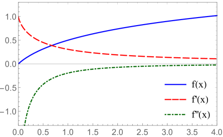
Figure 1: The figure shows the behavior of the functions $\bar{f}(x),\bar{f}^{\prime}(x)$ and $\bar{f}^{\prime\prime}(x)$ defined in Eqs. (2.21)-(2.25), where $f(x),f^{\prime}(x),f^{\prime\prime}(x)$ in the figure stand for $\bar{f}(x),\bar{f}^{\prime}(x)$, $\bar{f}^{\prime\prime}(x)$, respectively.

It is convenient to rewrite the tree part potential into the following form by picking up one particular representation, say ${\boldsymbol{R}}_{1}$, from ${\boldsymbol{R}}_{p}$’s:

$$V^{\text{tree}} =M^{2}_{{\boldsymbol{R}}_{1}}\,\mathop{\text{tr}}\bigl{(}\Phi^{\dagger}\Phi\bigr{)}+\sum_{p=2}^{n_{R}}(M^{2}_{{\boldsymbol{R}}_{p}}-M^{2}_{{\boldsymbol{R}}_{1}})\,\mathop{\text{tr}}\bigl{(}\Phi_{{\boldsymbol{R}}_{p}}^{{\dagger}}\Phi_{{\boldsymbol{R}}_{p}}\bigr{)}.$$ (2.28)

This is because $\Phi=\sum_{p}\Phi_{{\boldsymbol{R}}_{p}}$ is the general (unconstrained) symmetric $d\times d$ matrix which solely appears in the 1-loop part potential $V^{\text{1-loop}}$, while $\Phi_{{\boldsymbol{R}}_{p}}$’s are constrained matrices subject to non-trivial condition belonging to the irreducible representation ${\boldsymbol{R}}_{p}$, so satisfying the orthogonality $\mathop{\text{tr}}(\Phi^{\dagger}_{{\boldsymbol{R}}_{p}}\Phi_{{\boldsymbol{R}}_{p^{\prime}}})=0$ for $p\not=p^{\prime}$.

Whether a symmetry breaking pattern $G\rightarrow H$ is possible or not is found as follows. Expand each $G$-irreducible representation ${\boldsymbol{R}}_{p}$ into $H$-irreducible components ${\boldsymbol{r}}_{p}^{H(i)}$:

$${\boldsymbol{R}}_{p}=\sum_{i=1}^{n^{H}_{p}}{\boldsymbol{r}}_{p}^{H(i)}.$$ (2.29)

If there is an $H$-singlet contained in this decomposition for one $p$ or more, then the possibility for the breaking $G\rightarrow H$ exists. So assuming the non-zero VEV for all the $H$-singlets and identifying how those singlet VEV(’s) is contained in the scalars $\Phi_{{\boldsymbol{R}}_{p}}$, we can calculate the potential and find the potential values at the minimum points of the potential. We do this calculation for all possibilities of the subgroup $H$. Then we can find the true minimum, comparing those minimum values for all possible choices of $H$. To find the symmetry breaking that realizes the lowest minimum of the potential, we should note that the present potential $V(\Phi)$ in Eq.(2.6) consists of negative definite monotonically decreasing 1-loop potential $V^{\text{1-loop}}(\Phi^{\dagger}\Phi)=-\sum_{I}f(m_{I}^{2})$ and positive definite tree potential $\sum_{p}M^{2}_{{\boldsymbol{R}}_{p}}\mathop{\text{tr}}(\Phi^{\dagger}_{{\boldsymbol{R}}_{p}}\Phi_{{\boldsymbol{R}}_{p}})$. So, to realize the lower values of the potential, it is preferable that

$$\hbox{ 1. the number of massive fermions $\psi_{I}$ with $m_{I}^{2}\not=0$ is as large as possible}.$$

2. the condensation (nonvanishing VEV) $$\left\langle{\Phi_{{\boldsymbol{R}}_{p}}}\right\rangle$$ occurs in the direction of

$$\hskip 15.00002pt\hbox{stronger coupling channel ${{\boldsymbol{R}}_{p}}$, i.e., with smaller $M^{2}_{{\boldsymbol{R}}_{p}}$}.$$ (2.30)

To examine all the possibilities systematically, we consider all the maximal little groups for every $\Phi_{{\boldsymbol{R}}_{p}}$ where the maximal little groups of $\Phi_{{\boldsymbol{R}}_{p}}$ are defined as follows: The little group of the VEV $\left\langle{\Phi_{{\boldsymbol{R}}_{p}}}\right\rangle$ of the group $G$ is $H_{\left\langle{\Phi_{{\boldsymbol{R}}_{p}}}\right\rangle}$ defined in Eq. (1.3) for the vector $\phi=\left\langle{\Phi_{{\boldsymbol{R}}_{p}}}\right\rangle$, so that the VEV $\left\langle{\Phi_{{\boldsymbol{R}}_{p}}}\right\rangle$ belongs to an $H_{\left\langle{\Phi_{{\boldsymbol{R}}_{p}}}\right\rangle}$-singlet. As the VEV $\left\langle{\Phi_{{\boldsymbol{R}}_{p}}}\right\rangle$ changes, the little group $H_{\left\langle{\Phi_{{\boldsymbol{R}}_{p}}}\right\rangle}$ also changes. A little group $H$ of some VEV $\left\langle{\Phi_{{\boldsymbol{R}}_{p}}}\right\rangle_{0}$ is called maximal little group of $\Phi_{{\boldsymbol{R}}_{p}}$ if there are no VEV $\left\langle{\Phi_{{\boldsymbol{R}}_{p}}}\right\rangle$ whose little group $H_{\left\langle{\Phi_{{\boldsymbol{R}}_{p}}}\right\rangle}$ satisfies $G\supset H_{\left\langle{\Phi_{{\boldsymbol{R}}_{p}}}\right\rangle}\supset H$. For certain systems of restricted class of potentials of scalar fields, there is Michel’s conjecture[57, 30] which claims that the group symmetry can breaks down only to one of the maximal little groups of the considered scalar field $\Phi_{{\boldsymbol{R}}_{p}}$. Our system does not fall into such a restricted system, so that the lowest potential needs not be realized by one of the maximal little groups. But we can anyway consider the breaking possibilities starting with maximal little group cases, and consider their successive breakings into smaller subgroups if necessary in view of the above criterion (2.30).

3 $G=SU(N)$, ${\boldsymbol{R}}=\ {\vbox{\hrule height=0.5pt\hbox{\vrule width=0.5pt,height=8.0pt\kern 8.0pt\vrule width=0.5pt} \hrule height=0.5pt}}$ ; defining representation $\psi_{i}$ case

First consider the simplest case in which the fermion belongs to the defining representation ${\boldsymbol{R}}=\rule{8.0pt}{0.5pt}\hskip-8.0pt\rule{0.5pt}{8.0pt}\hskip 8.0pt\hskip-0.5pt\hskip-8.0pt\rule[8.0pt]{8.0pt}{0.5pt}\rule[8.0pt]{0.5pt}{0.5pt}\hskip-0.5pt\rule{0.5pt}{8.0pt}\hskip-0.5pt\,\$ of $G=SU(N)$; $\psi_{I}=\psi_{i}$. Then, $d:=\dim\rule{8.0pt}{0.5pt}\hskip-8.0pt\rule{0.5pt}{8.0pt}\hskip 8.0pt\hskip-0.5pt\hskip-8.0pt\rule[8.0pt]{8.0pt}{0.5pt}\rule[8.0pt]{0.5pt}{0.5pt}\hskip-0.5pt\rule{0.5pt}{8.0pt}\hskip-0.5pt\,=N$ and the irreducible decomposition of the symmetric product of ${\boldsymbol{R}}\times{\boldsymbol{R}}$ is now trivial, since ${\boldsymbol{R}}_{p}$ is unique:

$$(\rule{8.0pt}{0.5pt}\hskip-8.0pt\rule{0.5pt}{8.0pt}\hskip 8.0pt\hskip-0.5pt\hskip-8.0pt\rule[8.0pt]{8.0pt}{0.5pt}\rule[8.0pt]{0.5pt}{0.5pt}\hskip-0.5pt\rule{0.5pt}{8.0pt}\hskip-0.5pt\,\times\rule{8.0pt}{0.5pt}\hskip-8.0pt\rule{0.5pt}{8.0pt}\hskip 8.0pt\hskip-0.5pt\hskip-8.0pt\rule[8.0pt]{8.0pt}{0.5pt}\rule[8.0pt]{0.5pt}{0.5pt}\hskip-0.5pt\rule{0.5pt}{8.0pt}\hskip-0.5pt\,)_{\rm S}=\rule{8.0pt}{0.5pt}\hskip-8.0pt\rule{0.5pt}{8.0pt}\hskip 8.0pt\hskip-0.5pt\hskip-8.0pt\rule[8.0pt]{8.0pt}{0.5pt}\rule[8.0pt]{0.5pt}{0.5pt}\hskip-0.5pt\rule{0.5pt}{8.0pt}\hskip-0.5pt\rule{8.0pt}{0.5pt}\hskip-8.0pt\rule{0.5pt}{8.0pt}\hskip 8.0pt\hskip-0.5pt\hskip-8.0pt\rule[8.0pt]{8.0pt}{0.5pt}\rule[8.0pt]{0.5pt}{0.5pt}\hskip-0.5pt\rule{0.5pt}{8.0pt}\hskip-0.5pt\,\ .$$ (3.1)

So, in this case, the irreducible scalar $\Phi_{{\rule{4.0pt}{0.4pt}\hskip-4.0pt\rule{0.4pt}{4.0pt}\hskip 4.0pt\hskip-0.4pt\hskip-4.0pt\rule[4.0pt]{4.0pt}{0.4pt}\rule[4.0pt]{0.4pt}{0.4pt}\hskip-0.4pt\rule{0.4pt}{4.0pt}\hskip-0.4pt\rule{4.0pt}{0.4pt}\hskip-4.0pt\rule{0.4pt}{4.0pt}\hskip 4.0pt\hskip-0.4pt\hskip-4.0pt\rule[4.0pt]{4.0pt}{0.4pt}\rule[4.0pt]{0.4pt}{0.4pt}\hskip-0.4pt\rule{0.4pt}{4.0pt}\hskip-0.4pt}\,IJ}$ is identical with the general unconstrained symmetric complex $N\times N$ matrix $\Phi_{IJ}$, so that the leading order potential is given by

$$V^{\text{leading}}= \sum_{I=1}^{N}F(v_{I}^{2}\,;M^{2}_{\rule{4.0pt}{0.4pt}\hskip-4.0pt\rule{0.4pt}{4.0pt}\hskip 4.0pt\hskip-0.4pt\hskip-4.0pt\rule[4.0pt]{4.0pt}{0.4pt}\rule[4.0pt]{0.4pt}{0.4pt}\hskip-0.4pt\rule{0.4pt}{4.0pt}\hskip-0.4pt\rule{4.0pt}{0.4pt}\hskip-4.0pt\rule{0.4pt}{4.0pt}\hskip 4.0pt\hskip-0.4pt\hskip-4.0pt\rule[4.0pt]{4.0pt}{0.4pt}\rule[4.0pt]{0.4pt}{0.4pt}\hskip-0.4pt\rule{0.4pt}{4.0pt}\hskip-0.4pt}),$$

$$F(x\,;M^{2}):= M^{2}x-f(x),$$ (3.2)

where $v^{2}_{I}$ is the eigenvalues of the $d\times d$ Hermitian matrix $\Phi^{\dagger}\Phi$. The point here is that the $d$ eigenvalues $v^{2}_{I}$ are all independent and are independently determined by the minimum condition of the common function $F(x\,;M^{2}_{\rule{4.0pt}{0.4pt}\hskip-4.0pt\rule{0.4pt}{4.0pt}\hskip 4.0pt\hskip-0.4pt\hskip-4.0pt\rule[4.0pt]{4.0pt}{0.4pt}\rule[4.0pt]{0.4pt}{0.4pt}\hskip-0.4pt\rule{0.4pt}{4.0pt}\hskip-0.4pt\rule{4.0pt}{0.4pt}\hskip-4.0pt\rule{0.4pt}{4.0pt}\hskip 4.0pt\hskip-0.4pt\hskip-4.0pt\rule[4.0pt]{4.0pt}{0.4pt}\rule[4.0pt]{0.4pt}{0.4pt}\hskip-0.4pt\rule{0.4pt}{4.0pt}\hskip-0.4pt})$. Since the minimum point $x_{0}$ is uniquely fixed by $f^{\prime}(x_{0})=M^{2}_{\rule{4.0pt}{0.4pt}\hskip-4.0pt\rule{0.4pt}{4.0pt}\hskip 4.0pt\hskip-0.4pt\hskip-4.0pt\rule[4.0pt]{4.0pt}{0.4pt}\rule[4.0pt]{0.4pt}{0.4pt}\hskip-0.4pt\rule{0.4pt}{4.0pt}\hskip-0.4pt\rule{4.0pt}{0.4pt}\hskip-4.0pt\rule{0.4pt}{4.0pt}\hskip 4.0pt\hskip-0.4pt\hskip-4.0pt\rule[4.0pt]{4.0pt}{0.4pt}\rule[4.0pt]{0.4pt}{0.4pt}\hskip-0.4pt\rule{0.4pt}{4.0pt}\hskip-0.4pt}$, we can conclude that

$$v_{I}^{2}=x_{0}\ \ \hbox{for}\ \ \forall I\quad\rightarrow\quad\hbox{$N$ fermions $\psi_{I}$ all have a degenerate mass-square $x_{0}$}.$$ (3.3)

This common mass-square is, of course, non-vanishing only when $G_{{\rule{4.0pt}{0.4pt}\hskip-4.0pt\rule{0.4pt}{4.0pt}\hskip 4.0pt\hskip-0.4pt\hskip-4.0pt\rule[4.0pt]{4.0pt}{0.4pt}\rule[4.0pt]{0.4pt}{0.4pt}\hskip-0.4pt\rule{0.4pt}{4.0pt}\hskip-0.4pt\rule{4.0pt}{0.4pt}\hskip-4.0pt\rule{0.4pt}{4.0pt}\hskip 4.0pt\hskip-0.4pt\hskip-4.0pt\rule[4.0pt]{4.0pt}{0.4pt}\rule[4.0pt]{0.4pt}{0.4pt}\hskip-0.4pt\rule{0.4pt}{4.0pt}\hskip-0.4pt}}=1/M^{2}_{{\rule{4.0pt}{0.4pt}\hskip-4.0pt\rule{0.4pt}{4.0pt}\hskip 4.0pt\hskip-0.4pt\hskip-4.0pt\rule[4.0pt]{4.0pt}{0.4pt}\rule[4.0pt]{0.4pt}{0.4pt}\hskip-0.4pt\rule{0.4pt}{4.0pt}\hskip-0.4pt\rule{4.0pt}{0.4pt}\hskip-4.0pt\rule{0.4pt}{4.0pt}\hskip 4.0pt\hskip-0.4pt\hskip-4.0pt\rule[4.0pt]{4.0pt}{0.4pt}\rule[4.0pt]{0.4pt}{0.4pt}\hskip-0.4pt\rule{0.4pt}{4.0pt}\hskip-0.4pt}}$ is larger than the critical coupling $G_{\text{c}}=16\pi^{2}/\Lambda^{2}$. That is, as far as the dynamical spontaneous breaking occurs, the subgroup $H$ to which the $G=SU(N)$ is broken down must be such that

$$\begin{cases}\hbox{i)}&\ \hbox{$\rule{8.0pt}{0.5pt}\hskip-8.0pt\rule{0.5pt}{8.0pt}\hskip 8.0pt\hskip-0.5pt\hskip-8.0pt\rule[8.0pt]{8.0pt}{0.5pt}\rule[8.0pt]{0.5pt}{0.5pt}\hskip-0.5pt\rule{0.5pt}{8.0pt}\hskip-0.5pt\,$ of $SU(N)$ is also an $N$-plet under $H$};\\ \hbox{ii)}&\ \hbox{$\rule{8.0pt}{0.5pt}\hskip-8.0pt\rule{0.5pt}{8.0pt}\hskip 8.0pt\hskip-0.5pt\hskip-8.0pt\rule[8.0pt]{8.0pt}{0.5pt}\rule[8.0pt]{0.5pt}{0.5pt}\hskip-0.5pt\rule{0.5pt}{8.0pt}\hskip-0.5pt\rule{8.0pt}{0.5pt}\hskip-8.0pt\rule{0.5pt}{8.0pt}\hskip 8.0pt\hskip-0.5pt\hskip-8.0pt\rule[8.0pt]{8.0pt}{0.5pt}\rule[8.0pt]{0.5pt}{0.5pt}\hskip-0.5pt\rule{0.5pt}{8.0pt}\hskip-0.5pt\,$ of $SU(N)$ contains an $H$-singlet under $H$-irreducible decomposition}.\\ \end{cases}$$ (3.4)

The first condition alone already excludes the dynamical breaking into regular subgroup $H$! This is because, if $H$ is a regular subgroup of $SU(N)$, the defining representation           necessarily splits into plural $H$-irreducible representations. And, the special subgroups $H$ of $G=SU(N)$ satisfying this condition i) are only $SO(N)$ and $USp(N)$ (for only even $N$ cases for the latter), aside from very special subgroups like $SO(10)$ for the case of $G=SU(16)$. In any cases, it is only $SO(N)$ that can also satisfy the second condition ii), since the symmetric tensor $\Phi_{IJ}$ realizes the common mass $\langle\Phi_{IJ}\rangle\propto\delta_{IJ}$ for $\psi_{I}$ but $\delta_{IJ}$ is an invariant tensor only of $SO(N)$.

We thus conclude: For $G=SU(N)$ NJL theory with fermion $\psi_{I}$ in defining representation ${\boldsymbol{R}}=\rule{8.0pt}{0.5pt}\hskip-8.0pt\rule{0.5pt}{8.0pt}\hskip 8.0pt\hskip-0.5pt\hskip-8.0pt\rule[8.0pt]{8.0pt}{0.5pt}\rule[8.0pt]{0.5pt}{0.5pt}\hskip-0.5pt\rule{0.5pt}{8.0pt}\hskip-0.5pt\,$ , $SU(N)$ is spontaneously broken to the special subgroup $H=SO(N)$.

$$G=\hbox{$SU(N)$ NJL} \{\,\psi_{I}\,\}\in\rule{8.0pt}{0.5pt}\hskip-8.0pt\rule{0.5pt}{8.0pt}\hskip 8.0pt\hskip-0.5pt\hskip-8.0pt\rule[8.0pt]{8.0pt}{0.5pt}\rule[8.0pt]{0.5pt}{0.5pt}\hskip-0.5pt\rule{0.5pt}{8.0pt}\hskip-0.5pt\,:$$ with

$$G=SU(N) \rightarrow H=SO(N)$$

$$\psi_{I}\ \rule{8.0pt}{0.5pt}\hskip-8.0pt\rule{0.5pt}{8.0pt}\hskip 8.0pt\hskip-0.5pt\hskip-8.0pt\rule[8.0pt]{8.0pt}{0.5pt}\rule[8.0pt]{0.5pt}{0.5pt}\hskip-0.5pt\rule{0.5pt}{8.0pt}\hskip-0.5pt\,:\ \ \bf{N} \rightarrow \bf{N}$$

$$\Phi_{IJ}\ \rule{8.0pt}{0.5pt}\hskip-8.0pt\rule{0.5pt}{8.0pt}\hskip 8.0pt\hskip-0.5pt\hskip-8.0pt\rule[8.0pt]{8.0pt}{0.5pt}\rule[8.0pt]{0.5pt}{0.5pt}\hskip-0.5pt\rule{0.5pt}{8.0pt}\hskip-0.5pt\rule{8.0pt}{0.5pt}\hskip-8.0pt\rule{0.5pt}{8.0pt}\hskip 8.0pt\hskip-0.5pt\hskip-8.0pt\rule[8.0pt]{8.0pt}{0.5pt}\rule[8.0pt]{0.5pt}{0.5pt}\hskip-0.5pt\rule{0.5pt}{8.0pt}\hskip-0.5pt\,:\ \ \frac{\bf{N(N+1)}}{\bf 2} \rightarrow \overset{\mathop{\text{tr}}\Phi}{\bf{1}}+\overset{\Phi-\mathop{\text{tr}}\Phi/N}{\bf{(N-1)(N+2)/2}}$$ (3.5)

in which the $N$-plet fermion $\psi_{I}$ of $SU(N)$ becomes $N$-plet of $SO(N)$ and the $N(N+1)/2$ dimensional scalars $\Phi_{IJ}\in\rule{8.0pt}{0.5pt}\hskip-8.0pt\rule{0.5pt}{8.0pt}\hskip 8.0pt\hskip-0.5pt\hskip-8.0pt\rule[8.0pt]{8.0pt}{0.5pt}\rule[8.0pt]{0.5pt}{0.5pt}\hskip-0.5pt\rule{0.5pt}{8.0pt}\hskip-0.5pt\rule{8.0pt}{0.5pt}\hskip-8.0pt\rule{0.5pt}{8.0pt}\hskip 8.0pt\hskip-0.5pt\hskip-8.0pt\rule[8.0pt]{8.0pt}{0.5pt}\rule[8.0pt]{0.5pt}{0.5pt}\hskip-0.5pt\rule{0.5pt}{8.0pt}\hskip-0.5pt\,$ splits into an $SO(N)$ singlet trace part $\mathop{\text{tr}}\Phi=\sum_{I}\Phi_{II}$ and traceless symmetric part $\Phi_{IJ}-(1/N)\delta_{IJ}\mathop{\text{tr}}\Phi$ of dimension $N(N+1)/2-1=(N-1)(N+2)/2$; the latter scalars are the Nambu-Goldstone bosons for this breaking $SU(N)$ $\rightarrow$ $SO(N)$. Indeed, $\dim SU(N)-\dim SO(N)=(N^{2}-1)-N(N-1)/2=(N+2)(N-1)/2$.

Before closing this section, we note an interesting general conclusion valid for a special coupling case, which can be drawn from this simple example; that is, for the general NJL model with fermions of general irreducible representation ${\boldsymbol{R}}$, we always have dynamical breaking into a special subgroup, if the coupling constants $G_{{\boldsymbol{R}}_{p}}=1/M^{2}_{{\boldsymbol{R}}_{p}}$ for $G$-irreducible channels ${\boldsymbol{R}}_{p}$ are all degenerate (i.e., ${\boldsymbol{R}}_{p}$-independent). Indeed, in such a case, potential $V$ depends only on the unconstrained scalar $\Phi$ because of the identity (2.28), so that all the fermions get a common mass just in the same way as in the simplest model in this section.

4 $G=SU(N)$, ${\boldsymbol{R}}=\$              ; rank-2 anti-symmetric $\psi_{ij}$ case

Next consider the case where the fermion belongs to the rank-2 anti-symmetric representation ${\boldsymbol{R}}={\raisebox{-3.5pt}{\rule{7.0pt}{0.5pt}\hskip-7.0pt\rule{0.5pt}{7.0pt}\hskip 7.0pt\hskip-0.5pt\hskip-7.0pt\rule[7.0pt]{7.0pt}{0.5pt}\rule[7.0pt]{0.5pt}{0.5pt}\hskip-0.5pt\rule{0.5pt}{7.0pt}\hskip-0.5pt}\hskip-7.0pt\raisebox{3.5pt}{\rule{7.0pt}{0.5pt}\hskip-7.0pt\rule{0.5pt}{7.0pt}\hskip 7.0pt\hskip-0.5pt\hskip-7.0pt\rule[7.0pt]{7.0pt}{0.5pt}\rule[7.0pt]{0.5pt}{0.5pt}\hskip-0.5pt\rule{0.5pt}{7.0pt}\hskip-0.5pt}}\,$, so that the index $I$ now stands for the anti-symmetric pair $[ij]$ ($i,j=1,\cdots,N;N\geq 2$); $\psi_{I}=\psi_{ij}=-\psi_{ji}$. Then the fermion bilinear scalar $\Phi_{IJ}\sim\psi_{I}\psi_{J}$ gives symmetric product $({\boldsymbol{R}}\times{\boldsymbol{R}})_{\rm S}$ decomposed into the following two irreducible representations ${\boldsymbol{R}}_{p}$:

$$\left(\ {\raisebox{-3.5pt}{\rule{7.0pt}{0.5pt}\hskip-7.0pt\rule{0.5pt}{7.0pt}\hskip 7.0pt\hskip-0.5pt\hskip-7.0pt\rule[7.0pt]{7.0pt}{0.5pt}\rule[7.0pt]{0.5pt}{0.5pt}\hskip-0.5pt\rule{0.5pt}{7.0pt}\hskip-0.5pt}\hskip-7.0pt\raisebox{3.5pt}{\rule{7.0pt}{0.5pt}\hskip-7.0pt\rule{0.5pt}{7.0pt}\hskip 7.0pt\hskip-0.5pt\hskip-7.0pt\rule[7.0pt]{7.0pt}{0.5pt}\rule[7.0pt]{0.5pt}{0.5pt}\hskip-0.5pt\rule{0.5pt}{7.0pt}\hskip-0.5pt}}\,\times{\raisebox{-3.5pt}{\rule{7.0pt}{0.5pt}\hskip-7.0pt\rule{0.5pt}{7.0pt}\hskip 7.0pt\hskip-0.5pt\hskip-7.0pt\rule[7.0pt]{7.0pt}{0.5pt}\rule[7.0pt]{0.5pt}{0.5pt}\hskip-0.5pt\rule{0.5pt}{7.0pt}\hskip-0.5pt}\hskip-7.0pt\raisebox{3.5pt}{\rule{7.0pt}{0.5pt}\hskip-7.0pt\rule{0.5pt}{7.0pt}\hskip 7.0pt\hskip-0.5pt\hskip-7.0pt\rule[7.0pt]{7.0pt}{0.5pt}\rule[7.0pt]{0.5pt}{0.5pt}\hskip-0.5pt\rule{0.5pt}{7.0pt}\hskip-0.5pt}}\,\ \right)_{\rm S}=\ {\raisebox{-7.0pt}{\raisebox{-3.5pt}{\rule{7.0pt}{0.5pt}\hskip-7.0pt\rule{0.5pt}{7.0pt}\hskip 7.0pt\hskip-0.5pt\hskip-7.0pt\rule[7.0pt]{7.0pt}{0.5pt}\rule[7.0pt]{0.5pt}{0.5pt}\hskip-0.5pt\rule{0.5pt}{7.0pt}\hskip-0.5pt}\hskip-7.0pt\raisebox{3.5pt}{\rule{7.0pt}{0.5pt}\hskip-7.0pt\rule{0.5pt}{7.0pt}\hskip 7.0pt\hskip-0.5pt\hskip-7.0pt\rule[7.0pt]{7.0pt}{0.5pt}\rule[7.0pt]{0.5pt}{0.5pt}\hskip-0.5pt\rule{0.5pt}{7.0pt}\hskip-0.5pt}}\hskip-7.0pt\raisebox{7.0pt}{\raisebox{-3.5pt}{\rule{7.0pt}{0.5pt}\hskip-7.0pt\rule{0.5pt}{7.0pt}\hskip 7.0pt\hskip-0.5pt\hskip-7.0pt\rule[7.0pt]{7.0pt}{0.5pt}\rule[7.0pt]{0.5pt}{0.5pt}\hskip-0.5pt\rule{0.5pt}{7.0pt}\hskip-0.5pt}\hskip-7.0pt\raisebox{3.5pt}{\rule{7.0pt}{0.5pt}\hskip-7.0pt\rule{0.5pt}{7.0pt}\hskip 7.0pt\hskip-0.5pt\hskip-7.0pt\rule[7.0pt]{7.0pt}{0.5pt}\rule[7.0pt]{0.5pt}{0.5pt}\hskip-0.5pt\rule{0.5pt}{7.0pt}\hskip-0.5pt}}\,}\ +\ {\raisebox{-3.5pt}{\rule{7.0pt}{0.5pt}\hskip-7.0pt\rule{0.5pt}{7.0pt}\hskip 7.0pt\hskip-0.5pt\hskip-7.0pt\rule[7.0pt]{7.0pt}{0.5pt}\rule[7.0pt]{0.5pt}{0.5pt}\hskip-0.5pt\rule{0.5pt}{7.0pt}\hskip-0.5pt\rule{7.0pt}{0.5pt}\hskip-7.0pt\rule{0.5pt}{7.0pt}\hskip 7.0pt\hskip-0.5pt\hskip-7.0pt\rule[7.0pt]{7.0pt}{0.5pt}\rule[7.0pt]{0.5pt}{0.5pt}\hskip-0.5pt\rule{0.5pt}{7.0pt}\hskip-0.5pt}\hskip-14.0pt\raisebox{3.5pt}{\rule{7.0pt}{0.5pt}\hskip-7.0pt\rule{0.5pt}{7.0pt}\hskip 7.0pt\hskip-0.5pt\hskip-7.0pt\rule[7.0pt]{7.0pt}{0.5pt}\rule[7.0pt]{0.5pt}{0.5pt}\hskip-0.5pt\rule{0.5pt}{7.0pt}\hskip-0.5pt\rule{7.0pt}{0.5pt}\hskip-7.0pt\rule{0.5pt}{7.0pt}\hskip 7.0pt\hskip-0.5pt\hskip-7.0pt\rule[7.0pt]{7.0pt}{0.5pt}\rule[7.0pt]{0.5pt}{0.5pt}\hskip-0.5pt\rule{0.5pt}{7.0pt}\hskip-0.5pt}\,}\ .$$ (4.1)

Namely, we have two irreducible auxiliary scalar fields in this case:

$$\Phi_{{\raisebox{-3.0pt}{\raisebox{-1.5pt}{\rule{3.0pt}{0.4pt}\hskip-3.0pt\rule{0.4pt}{3.0pt}\hskip 3.0pt\hskip-0.4pt\hskip-3.0pt\rule[3.0pt]{3.0pt}{0.4pt}\rule[3.0pt]{0.4pt}{0.4pt}\hskip-0.4pt\rule{0.4pt}{3.0pt}\hskip-0.4pt}\hskip-3.0pt\raisebox{1.5pt}{\rule{3.0pt}{0.4pt}\hskip-3.0pt\rule{0.4pt}{3.0pt}\hskip 3.0pt\hskip-0.4pt\hskip-3.0pt\rule[3.0pt]{3.0pt}{0.4pt}\rule[3.0pt]{0.4pt}{0.4pt}\hskip-0.4pt\rule{0.4pt}{3.0pt}\hskip-0.4pt}}\hskip-3.0pt\raisebox{3.0pt}{\raisebox{-1.5pt}{\rule{3.0pt}{0.4pt}\hskip-3.0pt\rule{0.4pt}{3.0pt}\hskip 3.0pt\hskip-0.4pt\hskip-3.0pt\rule[3.0pt]{3.0pt}{0.4pt}\rule[3.0pt]{0.4pt}{0.4pt}\hskip-0.4pt\rule{0.4pt}{3.0pt}\hskip-0.4pt}\hskip-3.0pt\raisebox{1.5pt}{\rule{3.0pt}{0.4pt}\hskip-3.0pt\rule{0.4pt}{3.0pt}\hskip 3.0pt\hskip-0.4pt\hskip-3.0pt\rule[3.0pt]{3.0pt}{0.4pt}\rule[3.0pt]{0.4pt}{0.4pt}\hskip-0.4pt\rule{0.4pt}{3.0pt}\hskip-0.4pt}}}}{}_{\,ij,kl},\qquad\Phi_{{\raisebox{-1.5pt}{\rule{3.0pt}{0.4pt}\hskip-3.0pt\rule{0.4pt}{3.0pt}\hskip 3.0pt\hskip-0.4pt\hskip-3.0pt\rule[3.0pt]{3.0pt}{0.4pt}\rule[3.0pt]{0.4pt}{0.4pt}\hskip-0.4pt\rule{0.4pt}{3.0pt}\hskip-0.4pt\rule{3.0pt}{0.4pt}\hskip-3.0pt\rule{0.4pt}{3.0pt}\hskip 3.0pt\hskip-0.4pt\hskip-3.0pt\rule[3.0pt]{3.0pt}{0.4pt}\rule[3.0pt]{0.4pt}{0.4pt}\hskip-0.4pt\rule{0.4pt}{3.0pt}\hskip-0.4pt}\hskip-6.0pt\raisebox{1.5pt}{\rule{3.0pt}{0.4pt}\hskip-3.0pt\rule{0.4pt}{3.0pt}\hskip 3.0pt\hskip-0.4pt\hskip-3.0pt\rule[3.0pt]{3.0pt}{0.4pt}\rule[3.0pt]{0.4pt}{0.4pt}\hskip-0.4pt\rule{0.4pt}{3.0pt}\hskip-0.4pt\rule{3.0pt}{0.4pt}\hskip-3.0pt\rule{0.4pt}{3.0pt}\hskip 3.0pt\hskip-0.4pt\hskip-3.0pt\rule[3.0pt]{3.0pt}{0.4pt}\rule[3.0pt]{0.4pt}{0.4pt}\hskip-0.4pt\rule{0.4pt}{3.0pt}\hskip-0.4pt}}}{}_{\,ij,kl}.$$ (4.2)

There are the following six maximal little groups $H$ of $G=SU(N)$, under which these two $SU(N)$ irreducible scalars have $H$-singlet components listed in Table 2.

	Maximal little group $H$ of $SU(N)$	$H$-singlet in
1)	(Regular) $SU(2)\times SU(N-2)$  $(N\geq{2})$ case —
2)	(Regular) $SU(4)\times SU(N-4)$  $(N\geq{4})$ case
3)	(Special) $SO(N)$  $(N\geq 3)$ case
4)	(Special) $USp(N^{\prime})$ ( $N^{\prime}=2\left[\frac{N}{2}\right],\ N\geq 4$ ) case	and
5)	(Special) $SU(4)\times SU(2)$ case for $N=8$
6)	(Special) $SO(10)$ case for $N=16$

Table 2: Six maximal little groups $H$ of $SU(N)$ for two $SU(N)$                                   and                                   irreducible scalars possessing $H$-singlet. (Regular) or (Special) in front of each little group name denotes the distinction whether it is a regular or special subgroup of $SU(N)$. The case 4) for $N=3$ reduces to the case 1) (Regular) $SU(2)\simeq USp(2)$, so was excluded from there. For $N=5$, the case 4) $USp(4)$ is really the maximal little group of                                   , but not of                                   ; for the latter                                   , the maximal little group is the case 2) (Regular) $SU(4)$ which contains the $USp(4)$ as a subgroup.

As explained before, we start the analysis of the potential with these breakings into maximal little groups and consider the possibility of successive breakings into further smaller subgroups when necessary.

First, we consider symmetry breaking of the cases 1), 3), 5), and 6) since their breakings are caused by the                                   condensation alone, so, independent of the coupling constant $G_{{\raisebox{-3.0pt}{\raisebox{-1.5pt}{\rule{3.0pt}{0.4pt}\hskip-3.0pt\rule{0.4pt}{3.0pt}\hskip 3.0pt\hskip-0.4pt\hskip-3.0pt\rule[3.0pt]{3.0pt}{0.4pt}\rule[3.0pt]{0.4pt}{0.4pt}\hskip-0.4pt\rule{0.4pt}{3.0pt}\hskip-0.4pt}\hskip-3.0pt\raisebox{1.5pt}{\rule{3.0pt}{0.4pt}\hskip-3.0pt\rule{0.4pt}{3.0pt}\hskip 3.0pt\hskip-0.4pt\hskip-3.0pt\rule[3.0pt]{3.0pt}{0.4pt}\rule[3.0pt]{0.4pt}{0.4pt}\hskip-0.4pt\rule{0.4pt}{3.0pt}\hskip-0.4pt}}\hskip-3.0pt\raisebox{3.0pt}{\raisebox{-1.5pt}{\rule{3.0pt}{0.4pt}\hskip-3.0pt\rule{0.4pt}{3.0pt}\hskip 3.0pt\hskip-0.4pt\hskip-3.0pt\rule[3.0pt]{3.0pt}{0.4pt}\rule[3.0pt]{0.4pt}{0.4pt}\hskip-0.4pt\rule{0.4pt}{3.0pt}\hskip-0.4pt}\hskip-3.0pt\raisebox{1.5pt}{\rule{3.0pt}{0.4pt}\hskip-3.0pt\rule{0.4pt}{3.0pt}\hskip 3.0pt\hskip-0.4pt\hskip-3.0pt\rule[3.0pt]{3.0pt}{0.4pt}\rule[3.0pt]{0.4pt}{0.4pt}\hskip-0.4pt\rule{0.4pt}{3.0pt}\hskip-0.4pt}}}}=M^{-2}_{{\raisebox{-3.0pt}{\raisebox{-1.5pt}{\rule{3.0pt}{0.4pt}\hskip-3.0pt\rule{0.4pt}{3.0pt}\hskip 3.0pt\hskip-0.4pt\hskip-3.0pt\rule[3.0pt]{3.0pt}{0.4pt}\rule[3.0pt]{0.4pt}{0.4pt}\hskip-0.4pt\rule{0.4pt}{3.0pt}\hskip-0.4pt}\hskip-3.0pt\raisebox{1.5pt}{\rule{3.0pt}{0.4pt}\hskip-3.0pt\rule{0.4pt}{3.0pt}\hskip 3.0pt\hskip-0.4pt\hskip-3.0pt\rule[3.0pt]{3.0pt}{0.4pt}\rule[3.0pt]{0.4pt}{0.4pt}\hskip-0.4pt\rule{0.4pt}{3.0pt}\hskip-0.4pt}}\hskip-3.0pt\raisebox{3.0pt}{\raisebox{-1.5pt}{\rule{3.0pt}{0.4pt}\hskip-3.0pt\rule{0.4pt}{3.0pt}\hskip 3.0pt\hskip-0.4pt\hskip-3.0pt\rule[3.0pt]{3.0pt}{0.4pt}\rule[3.0pt]{0.4pt}{0.4pt}\hskip-0.4pt\rule{0.4pt}{3.0pt}\hskip-0.4pt}\hskip-3.0pt\raisebox{1.5pt}{\rule{3.0pt}{0.4pt}\hskip-3.0pt\rule{0.4pt}{3.0pt}\hskip 3.0pt\hskip-0.4pt\hskip-3.0pt\rule[3.0pt]{3.0pt}{0.4pt}\rule[3.0pt]{0.4pt}{0.4pt}\hskip-0.4pt\rule{0.4pt}{3.0pt}\hskip-0.4pt}}}}$. As far as the coupling constant $G_{{\raisebox{-1.5pt}{\rule{3.0pt}{0.4pt}\hskip-3.0pt\rule{0.4pt}{3.0pt}\hskip 3.0pt\hskip-0.4pt\hskip-3.0pt\rule[3.0pt]{3.0pt}{0.4pt}\rule[3.0pt]{0.4pt}{0.4pt}\hskip-0.4pt\rule{0.4pt}{3.0pt}\hskip-0.4pt\rule{3.0pt}{0.4pt}\hskip-3.0pt\rule{0.4pt}{3.0pt}\hskip 3.0pt\hskip-0.4pt\hskip-3.0pt\rule[3.0pt]{3.0pt}{0.4pt}\rule[3.0pt]{0.4pt}{0.4pt}\hskip-0.4pt\rule{0.4pt}{3.0pt}\hskip-0.4pt}\hskip-6.0pt\raisebox{1.5pt}{\rule{3.0pt}{0.4pt}\hskip-3.0pt\rule{0.4pt}{3.0pt}\hskip 3.0pt\hskip-0.4pt\hskip-3.0pt\rule[3.0pt]{3.0pt}{0.4pt}\rule[3.0pt]{0.4pt}{0.4pt}\hskip-0.4pt\rule{0.4pt}{3.0pt}\hskip-0.4pt\rule{3.0pt}{0.4pt}\hskip-3.0pt\rule{0.4pt}{3.0pt}\hskip 3.0pt\hskip-0.4pt\hskip-3.0pt\rule[3.0pt]{3.0pt}{0.4pt}\rule[3.0pt]{0.4pt}{0.4pt}\hskip-0.4pt\rule{0.4pt}{3.0pt}\hskip-0.4pt}}}=M^{-2}_{{\raisebox{-1.5pt}{\rule{3.0pt}{0.4pt}\hskip-3.0pt\rule{0.4pt}{3.0pt}\hskip 3.0pt\hskip-0.4pt\hskip-3.0pt\rule[3.0pt]{3.0pt}{0.4pt}\rule[3.0pt]{0.4pt}{0.4pt}\hskip-0.4pt\rule{0.4pt}{3.0pt}\hskip-0.4pt\rule{3.0pt}{0.4pt}\hskip-3.0pt\rule{0.4pt}{3.0pt}\hskip 3.0pt\hskip-0.4pt\hskip-3.0pt\rule[3.0pt]{3.0pt}{0.4pt}\rule[3.0pt]{0.4pt}{0.4pt}\hskip-0.4pt\rule{0.4pt}{3.0pt}\hskip-0.4pt}\hskip-6.0pt\raisebox{1.5pt}{\rule{3.0pt}{0.4pt}\hskip-3.0pt\rule{0.4pt}{3.0pt}\hskip 3.0pt\hskip-0.4pt\hskip-3.0pt\rule[3.0pt]{3.0pt}{0.4pt}\rule[3.0pt]{0.4pt}{0.4pt}\hskip-0.4pt\rule{0.4pt}{3.0pt}\hskip-0.4pt\rule{3.0pt}{0.4pt}\hskip-3.0pt\rule{0.4pt}{3.0pt}\hskip 3.0pt\hskip-0.4pt\hskip-3.0pt\rule[3.0pt]{3.0pt}{0.4pt}\rule[3.0pt]{0.4pt}{0.4pt}\hskip-0.4pt\rule{0.4pt}{3.0pt}\hskip-0.4pt}}}$ is larger than its critical coupling, we can compare the potential energies for those breaking cases with one another irrespectively of the coupling strength $G_{{\raisebox{-1.5pt}{\rule{3.0pt}{0.4pt}\hskip-3.0pt\rule{0.4pt}{3.0pt}\hskip 3.0pt\hskip-0.4pt\hskip-3.0pt\rule[3.0pt]{3.0pt}{0.4pt}\rule[3.0pt]{0.4pt}{0.4pt}\hskip-0.4pt\rule{0.4pt}{3.0pt}\hskip-0.4pt\rule{3.0pt}{0.4pt}\hskip-3.0pt\rule{0.4pt}{3.0pt}\hskip 3.0pt\hskip-0.4pt\hskip-3.0pt\rule[3.0pt]{3.0pt}{0.4pt}\rule[3.0pt]{0.4pt}{0.4pt}\hskip-0.4pt\rule{0.4pt}{3.0pt}\hskip-0.4pt}\hskip-6.0pt\raisebox{1.5pt}{\rule{3.0pt}{0.4pt}\hskip-3.0pt\rule{0.4pt}{3.0pt}\hskip 3.0pt\hskip-0.4pt\hskip-3.0pt\rule[3.0pt]{3.0pt}{0.4pt}\rule[3.0pt]{0.4pt}{0.4pt}\hskip-0.4pt\rule{0.4pt}{3.0pt}\hskip-0.4pt\rule{3.0pt}{0.4pt}\hskip-3.0pt\rule{0.4pt}{3.0pt}\hskip 3.0pt\hskip-0.4pt\hskip-3.0pt\rule[3.0pt]{3.0pt}{0.4pt}\rule[3.0pt]{0.4pt}{0.4pt}\hskip-0.4pt\rule{0.4pt}{3.0pt}\hskip-0.4pt}}}$ . From Tables 3 and 4, we see that the original fermion ${N(N-1)\over 2}$plet                  , $\psi_{I}=\psi_{ij}$, of $G=SU(N)$ is also an $H$-irreducible ${N(N-1)\over 2}$plet in the case 3) $H=SO(N)$, and also in the very special case 6) of $N=16$, $H=SO(10)$. The potential for those cases is clearly given by, for any $N$,

$$V_{{SO(N)}}(V) =\frac{N(N-1)}{2}F(V^{2}\,;M_{{\raisebox{-1.5pt}{\rule{3.0pt}{0.4pt}\hskip-3.0pt\rule{0.4pt}{3.0pt}\hskip 3.0pt\hskip-0.4pt\hskip-3.0pt\rule[3.0pt]{3.0pt}{0.4pt}\rule[3.0pt]{0.4pt}{0.4pt}\hskip-0.4pt\rule{0.4pt}{3.0pt}\hskip-0.4pt\rule{3.0pt}{0.4pt}\hskip-3.0pt\rule{0.4pt}{3.0pt}\hskip 3.0pt\hskip-0.4pt\hskip-3.0pt\rule[3.0pt]{3.0pt}{0.4pt}\rule[3.0pt]{0.4pt}{0.4pt}\hskip-0.4pt\rule{0.4pt}{3.0pt}\hskip-0.4pt}\hskip-6.0pt\raisebox{1.5pt}{\rule{3.0pt}{0.4pt}\hskip-3.0pt\rule{0.4pt}{3.0pt}\hskip 3.0pt\hskip-0.4pt\hskip-3.0pt\rule[3.0pt]{3.0pt}{0.4pt}\rule[3.0pt]{0.4pt}{0.4pt}\hskip-0.4pt\rule{0.4pt}{3.0pt}\hskip-0.4pt\rule{3.0pt}{0.4pt}\hskip-3.0pt\rule{0.4pt}{3.0pt}\hskip 3.0pt\hskip-0.4pt\hskip-3.0pt\rule[3.0pt]{3.0pt}{0.4pt}\rule[3.0pt]{0.4pt}{0.4pt}\hskip-0.4pt\rule{0.4pt}{3.0pt}\hskip-0.4pt}}}^{2})=\frac{N(N-1)}{2}\bigl{(}M_{{\raisebox{-1.5pt}{\rule{3.0pt}{0.4pt}\hskip-3.0pt\rule{0.4pt}{3.0pt}\hskip 3.0pt\hskip-0.4pt\hskip-3.0pt\rule[3.0pt]{3.0pt}{0.4pt}\rule[3.0pt]{0.4pt}{0.4pt}\hskip-0.4pt\rule{0.4pt}{3.0pt}\hskip-0.4pt\rule{3.0pt}{0.4pt}\hskip-3.0pt\rule{0.4pt}{3.0pt}\hskip 3.0pt\hskip-0.4pt\hskip-3.0pt\rule[3.0pt]{3.0pt}{0.4pt}\rule[3.0pt]{0.4pt}{0.4pt}\hskip-0.4pt\rule{0.4pt}{3.0pt}\hskip-0.4pt}\hskip-6.0pt\raisebox{1.5pt}{\rule{3.0pt}{0.4pt}\hskip-3.0pt\rule{0.4pt}{3.0pt}\hskip 3.0pt\hskip-0.4pt\hskip-3.0pt\rule[3.0pt]{3.0pt}{0.4pt}\rule[3.0pt]{0.4pt}{0.4pt}\hskip-0.4pt\rule{0.4pt}{3.0pt}\hskip-0.4pt\rule{3.0pt}{0.4pt}\hskip-3.0pt\rule{0.4pt}{3.0pt}\hskip 3.0pt\hskip-0.4pt\hskip-3.0pt\rule[3.0pt]{3.0pt}{0.4pt}\rule[3.0pt]{0.4pt}{0.4pt}\hskip-0.4pt\rule{0.4pt}{3.0pt}\hskip-0.4pt}}}^{2}V^{2}-f(V^{2})\bigr{)};$$ (4.3)

for $N=16$,

$$V_{{SO(16)}}(V)=V_{{SO(10)}}(V)=120F(V^{2}\,;M_{{\raisebox{-1.5pt}{\rule{3.0pt}{0.4pt}\hskip-3.0pt\rule{0.4pt}{3.0pt}\hskip 3.0pt\hskip-0.4pt\hskip-3.0pt\rule[3.0pt]{3.0pt}{0.4pt}\rule[3.0pt]{0.4pt}{0.4pt}\hskip-0.4pt\rule{0.4pt}{3.0pt}\hskip-0.4pt\rule{3.0pt}{0.4pt}\hskip-3.0pt\rule{0.4pt}{3.0pt}\hskip 3.0pt\hskip-0.4pt\hskip-3.0pt\rule[3.0pt]{3.0pt}{0.4pt}\rule[3.0pt]{0.4pt}{0.4pt}\hskip-0.4pt\rule{0.4pt}{3.0pt}\hskip-0.4pt}\hskip-6.0pt\raisebox{1.5pt}{\rule{3.0pt}{0.4pt}\hskip-3.0pt\rule{0.4pt}{3.0pt}\hskip 3.0pt\hskip-0.4pt\hskip-3.0pt\rule[3.0pt]{3.0pt}{0.4pt}\rule[3.0pt]{0.4pt}{0.4pt}\hskip-0.4pt\rule{0.4pt}{3.0pt}\hskip-0.4pt\rule{3.0pt}{0.4pt}\hskip-3.0pt\rule{0.4pt}{3.0pt}\hskip 3.0pt\hskip-0.4pt\hskip-3.0pt\rule[3.0pt]{3.0pt}{0.4pt}\rule[3.0pt]{0.4pt}{0.4pt}\hskip-0.4pt\rule{0.4pt}{3.0pt}\hskip-0.4pt}}}^{2})=120\bigl{(}M_{{\raisebox{-1.5pt}{\rule{3.0pt}{0.4pt}\hskip-3.0pt\rule{0.4pt}{3.0pt}\hskip 3.0pt\hskip-0.4pt\hskip-3.0pt\rule[3.0pt]{3.0pt}{0.4pt}\rule[3.0pt]{0.4pt}{0.4pt}\hskip-0.4pt\rule{0.4pt}{3.0pt}\hskip-0.4pt\rule{3.0pt}{0.4pt}\hskip-3.0pt\rule{0.4pt}{3.0pt}\hskip 3.0pt\hskip-0.4pt\hskip-3.0pt\rule[3.0pt]{3.0pt}{0.4pt}\rule[3.0pt]{0.4pt}{0.4pt}\hskip-0.4pt\rule{0.4pt}{3.0pt}\hskip-0.4pt}\hskip-6.0pt\raisebox{1.5pt}{\rule{3.0pt}{0.4pt}\hskip-3.0pt\rule{0.4pt}{3.0pt}\hskip 3.0pt\hskip-0.4pt\hskip-3.0pt\rule[3.0pt]{3.0pt}{0.4pt}\rule[3.0pt]{0.4pt}{0.4pt}\hskip-0.4pt\rule{0.4pt}{3.0pt}\hskip-0.4pt\rule{3.0pt}{0.4pt}\hskip-3.0pt\rule{0.4pt}{3.0pt}\hskip 3.0pt\hskip-0.4pt\hskip-3.0pt\rule[3.0pt]{3.0pt}{0.4pt}\rule[3.0pt]{0.4pt}{0.4pt}\hskip-0.4pt\rule{0.4pt}{3.0pt}\hskip-0.4pt}}}^{2}V^{2}-f(V^{2})\bigr{)}.$$ (4.4)

Since $V^{2}$ can be chosen to be the minimum of the function $F(V^{2}\,;M_{{\raisebox{-1.5pt}{\rule{3.0pt}{0.4pt}\hskip-3.0pt\rule{0.4pt}{3.0pt}\hskip 3.0pt\hskip-0.4pt\hskip-3.0pt\rule[3.0pt]{3.0pt}{0.4pt}\rule[3.0pt]{0.4pt}{0.4pt}\hskip-0.4pt\rule{0.4pt}{3.0pt}\hskip-0.4pt\rule{3.0pt}{0.4pt}\hskip-3.0pt\rule{0.4pt}{3.0pt}\hskip 3.0pt\hskip-0.4pt\hskip-3.0pt\rule[3.0pt]{3.0pt}{0.4pt}\rule[3.0pt]{0.4pt}{0.4pt}\hskip-0.4pt\rule{0.4pt}{3.0pt}\hskip-0.4pt}\hskip-6.0pt\raisebox{1.5pt}{\rule{3.0pt}{0.4pt}\hskip-3.0pt\rule{0.4pt}{3.0pt}\hskip 3.0pt\hskip-0.4pt\hskip-3.0pt\rule[3.0pt]{3.0pt}{0.4pt}\rule[3.0pt]{0.4pt}{0.4pt}\hskip-0.4pt\rule{0.4pt}{3.0pt}\hskip-0.4pt\rule{3.0pt}{0.4pt}\hskip-3.0pt\rule{0.4pt}{3.0pt}\hskip 3.0pt\hskip-0.4pt\hskip-3.0pt\rule[3.0pt]{3.0pt}{0.4pt}\rule[3.0pt]{0.4pt}{0.4pt}\hskip-0.4pt\rule{0.4pt}{3.0pt}\hskip-0.4pt}}}^{2})$, then this potential clearly realizes the lowest possible value for the breakings into this channel scalar $\Phi_{{\raisebox{-1.5pt}{\rule{3.0pt}{0.4pt}\hskip-3.0pt\rule{0.4pt}{3.0pt}\hskip 3.0pt\hskip-0.4pt\hskip-3.0pt\rule[3.0pt]{3.0pt}{0.4pt}\rule[3.0pt]{0.4pt}{0.4pt}\hskip-0.4pt\rule{0.4pt}{3.0pt}\hskip-0.4pt\rule{3.0pt}{0.4pt}\hskip-3.0pt\rule{0.4pt}{3.0pt}\hskip 3.0pt\hskip-0.4pt\hskip-3.0pt\rule[3.0pt]{3.0pt}{0.4pt}\rule[3.0pt]{0.4pt}{0.4pt}\hskip-0.4pt\rule{0.4pt}{3.0pt}\hskip-0.4pt}\hskip-6.0pt\raisebox{1.5pt}{\rule{3.0pt}{0.4pt}\hskip-3.0pt\rule{0.4pt}{3.0pt}\hskip 3.0pt\hskip-0.4pt\hskip-3.0pt\rule[3.0pt]{3.0pt}{0.4pt}\rule[3.0pt]{0.4pt}{0.4pt}\hskip-0.4pt\rule{0.4pt}{3.0pt}\hskip-0.4pt\rule{3.0pt}{0.4pt}\hskip-3.0pt\rule{0.4pt}{3.0pt}\hskip 3.0pt\hskip-0.4pt\hskip-3.0pt\rule[3.0pt]{3.0pt}{0.4pt}\rule[3.0pt]{0.4pt}{0.4pt}\hskip-0.4pt\rule{0.4pt}{3.0pt}\hskip-0.4pt}}}$. We can thus forget about the other possibilities of 1) and 5), henceforth.

For the other coupling strength cases, $M^{2}_{{\raisebox{-3.0pt}{\raisebox{-1.5pt}{\rule{3.0pt}{0.4pt}\hskip-3.0pt\rule{0.4pt}{3.0pt}\hskip 3.0pt\hskip-0.4pt\hskip-3.0pt\rule[3.0pt]{3.0pt}{0.4pt}\rule[3.0pt]{0.4pt}{0.4pt}\hskip-0.4pt\rule{0.4pt}{3.0pt}\hskip-0.4pt}\hskip-3.0pt\raisebox{1.5pt}{\rule{3.0pt}{0.4pt}\hskip-3.0pt\rule{0.4pt}{3.0pt}\hskip 3.0pt\hskip-0.4pt\hskip-3.0pt\rule[3.0pt]{3.0pt}{0.4pt}\rule[3.0pt]{0.4pt}{0.4pt}\hskip-0.4pt\rule{0.4pt}{3.0pt}\hskip-0.4pt}}\hskip-3.0pt\raisebox{3.0pt}{\raisebox{-1.5pt}{\rule{3.0pt}{0.4pt}\hskip-3.0pt\rule{0.4pt}{3.0pt}\hskip 3.0pt\hskip-0.4pt\hskip-3.0pt\rule[3.0pt]{3.0pt}{0.4pt}\rule[3.0pt]{0.4pt}{0.4pt}\hskip-0.4pt\rule{0.4pt}{3.0pt}\hskip-0.4pt}\hskip-3.0pt\raisebox{1.5pt}{\rule{3.0pt}{0.4pt}\hskip-3.0pt\rule{0.4pt}{3.0pt}\hskip 3.0pt\hskip-0.4pt\hskip-3.0pt\rule[3.0pt]{3.0pt}{0.4pt}\rule[3.0pt]{0.4pt}{0.4pt}\hskip-0.4pt\rule{0.4pt}{3.0pt}\hskip-0.4pt}}}}\leq M^{2}_{{\raisebox{-1.5pt}{\rule{3.0pt}{0.4pt}\hskip-3.0pt\rule{0.4pt}{3.0pt}\hskip 3.0pt\hskip-0.4pt\hskip-3.0pt\rule[3.0pt]{3.0pt}{0.4pt}\rule[3.0pt]{0.4pt}{0.4pt}\hskip-0.4pt\rule{0.4pt}{3.0pt}\hskip-0.4pt\rule{3.0pt}{0.4pt}\hskip-3.0pt\rule{0.4pt}{3.0pt}\hskip 3.0pt\hskip-0.4pt\hskip-3.0pt\rule[3.0pt]{3.0pt}{0.4pt}\rule[3.0pt]{0.4pt}{0.4pt}\hskip-0.4pt\rule{0.4pt}{3.0pt}\hskip-0.4pt}\hskip-6.0pt\raisebox{1.5pt}{\rule{3.0pt}{0.4pt}\hskip-3.0pt\rule{0.4pt}{3.0pt}\hskip 3.0pt\hskip-0.4pt\hskip-3.0pt\rule[3.0pt]{3.0pt}{0.4pt}\rule[3.0pt]{0.4pt}{0.4pt}\hskip-0.4pt\rule{0.4pt}{3.0pt}\hskip-0.4pt\rule{3.0pt}{0.4pt}\hskip-3.0pt\rule{0.4pt}{3.0pt}\hskip 3.0pt\hskip-0.4pt\hskip-3.0pt\rule[3.0pt]{3.0pt}{0.4pt}\rule[3.0pt]{0.4pt}{0.4pt}\hskip-0.4pt\rule{0.4pt}{3.0pt}\hskip-0.4pt}}}$, we need to consider the condensations into the channel $\Phi_{{\raisebox{-3.0pt}{\raisebox{-1.5pt}{\rule{3.0pt}{0.4pt}\hskip-3.0pt\rule{0.4pt}{3.0pt}\hskip 3.0pt\hskip-0.4pt\hskip-3.0pt\rule[3.0pt]{3.0pt}{0.4pt}\rule[3.0pt]{0.4pt}{0.4pt}\hskip-0.4pt\rule{0.4pt}{3.0pt}\hskip-0.4pt}\hskip-3.0pt\raisebox{1.5pt}{\rule{3.0pt}{0.4pt}\hskip-3.0pt\rule{0.4pt}{3.0pt}\hskip 3.0pt\hskip-0.4pt\hskip-3.0pt\rule[3.0pt]{3.0pt}{0.4pt}\rule[3.0pt]{0.4pt}{0.4pt}\hskip-0.4pt\rule{0.4pt}{3.0pt}\hskip-0.4pt}}\hskip-3.0pt\raisebox{3.0pt}{\raisebox{-1.5pt}{\rule{3.0pt}{0.4pt}\hskip-3.0pt\rule{0.4pt}{3.0pt}\hskip 3.0pt\hskip-0.4pt\hskip-3.0pt\rule[3.0pt]{3.0pt}{0.4pt}\rule[3.0pt]{0.4pt}{0.4pt}\hskip-0.4pt\rule{0.4pt}{3.0pt}\hskip-0.4pt}\hskip-3.0pt\raisebox{1.5pt}{\rule{3.0pt}{0.4pt}\hskip-3.0pt\rule{0.4pt}{3.0pt}\hskip 3.0pt\hskip-0.4pt\hskip-3.0pt\rule[3.0pt]{3.0pt}{0.4pt}\rule[3.0pt]{0.4pt}{0.4pt}\hskip-0.4pt\rule{0.4pt}{3.0pt}\hskip-0.4pt}}}}$ also and evaluate the potential in more detail by identifying the explicit form of the scalar VEVs. So let us now turn to this task.

4.1 Scalar VEV and potential for each case

Here we identify the explicit form of the scalar VEVs for the cases 2), 3), 4), and 6) one by one to evaluate the potential in detail.

2) For the regular breaking case 2) into $H=SU(4)\times SU(N-4)$ $(N\geq{4})$, the $H$-singlet scalar is contained only in $\Phi_{{\raisebox{-3.0pt}{\raisebox{-1.5pt}{\rule{3.0pt}{0.4pt}\hskip-3.0pt\rule{0.4pt}{3.0pt}\hskip 3.0pt\hskip-0.4pt\hskip-3.0pt\rule[3.0pt]{3.0pt}{0.4pt}\rule[3.0pt]{0.4pt}{0.4pt}\hskip-0.4pt\rule{0.4pt}{3.0pt}\hskip-0.4pt}\hskip-3.0pt\raisebox{1.5pt}{\rule{3.0pt}{0.4pt}\hskip-3.0pt\rule{0.4pt}{3.0pt}\hskip 3.0pt\hskip-0.4pt\hskip-3.0pt\rule[3.0pt]{3.0pt}{0.4pt}\rule[3.0pt]{0.4pt}{0.4pt}\hskip-0.4pt\rule{0.4pt}{3.0pt}\hskip-0.4pt}}\hskip-3.0pt\raisebox{3.0pt}{\raisebox{-1.5pt}{\rule{3.0pt}{0.4pt}\hskip-3.0pt\rule{0.4pt}{3.0pt}\hskip 3.0pt\hskip-0.4pt\hskip-3.0pt\rule[3.0pt]{3.0pt}{0.4pt}\rule[3.0pt]{0.4pt}{0.4pt}\hskip-0.4pt\rule{0.4pt}{3.0pt}\hskip-0.4pt}\hskip-3.0pt\raisebox{1.5pt}{\rule{3.0pt}{0.4pt}\hskip-3.0pt\rule{0.4pt}{3.0pt}\hskip 3.0pt\hskip-0.4pt\hskip-3.0pt\rule[3.0pt]{3.0pt}{0.4pt}\rule[3.0pt]{0.4pt}{0.4pt}\hskip-0.4pt\rule{0.4pt}{3.0pt}\hskip-0.4pt}}}}$ and the VEV takes the form:

$$\bigl{\langle}\Phi_{{\raisebox{-3.0pt}{\raisebox{-1.5pt}{\rule{3.0pt}{0.4pt}\hskip-3.0pt\rule{0.4pt}{3.0pt}\hskip 3.0pt\hskip-0.4pt\hskip-3.0pt\rule[3.0pt]{3.0pt}{0.4pt}\rule[3.0pt]{0.4pt}{0.4pt}\hskip-0.4pt\rule{0.4pt}{3.0pt}\hskip-0.4pt}\hskip-3.0pt\raisebox{1.5pt}{\rule{3.0pt}{0.4pt}\hskip-3.0pt\rule{0.4pt}{3.0pt}\hskip 3.0pt\hskip-0.4pt\hskip-3.0pt\rule[3.0pt]{3.0pt}{0.4pt}\rule[3.0pt]{0.4pt}{0.4pt}\hskip-0.4pt\rule{0.4pt}{3.0pt}\hskip-0.4pt}}\hskip-3.0pt\raisebox{3.0pt}{\raisebox{-1.5pt}{\rule{3.0pt}{0.4pt}\hskip-3.0pt\rule{0.4pt}{3.0pt}\hskip 3.0pt\hskip-0.4pt\hskip-3.0pt\rule[3.0pt]{3.0pt}{0.4pt}\rule[3.0pt]{0.4pt}{0.4pt}\hskip-0.4pt\rule{0.4pt}{3.0pt}\hskip-0.4pt}\hskip-3.0pt\raisebox{1.5pt}{\rule{3.0pt}{0.4pt}\hskip-3.0pt\rule{0.4pt}{3.0pt}\hskip 3.0pt\hskip-0.4pt\hskip-3.0pt\rule[3.0pt]{3.0pt}{0.4pt}\rule[3.0pt]{0.4pt}{0.4pt}\hskip-0.4pt\rule{0.4pt}{3.0pt}\hskip-0.4pt}}}}{}_{\,ij,kl}\bigr{\rangle}=\frac{1}{2\cdot 2}\,v\,\epsilon_{ijkl56\cdots N},$$ (4.5)

where $\epsilon_{ijkl56\cdots N}$ is a rank-$N$ totally anti-symmetric tensor of $SU(N)$ so that it is non-vanishing only when the first four indices $i,j,k,l$ all take the values 1 to 4 belonging to the $SU(4)$ subgroup. This VEV (4.5) gives the following form of fermion mass matrix for the 6 independent components $\psi_{i<j}$ ($1\leq i<j\leq 4$) $\{\,\psi_{12},\,\psi_{34},\,\psi_{13},\,\psi_{24},\,\psi_{14},\,\psi_{23}\,\}\in{\raisebox{-3.5pt}{\rule{7.0pt}{0.5pt}\hskip-7.0pt\rule{0.5pt}{7.0pt}\hskip 7.0pt\hskip-0.5pt\hskip-7.0pt\rule[7.0pt]{7.0pt}{0.5pt}\rule[7.0pt]{0.5pt}{0.5pt}\hskip-0.5pt\rule{0.5pt}{7.0pt}\hskip-0.5pt}\hskip-7.0pt\raisebox{3.5pt}{\rule{7.0pt}{0.5pt}\hskip-7.0pt\rule{0.5pt}{7.0pt}\hskip 7.0pt\hskip-0.5pt\hskip-7.0pt\rule[7.0pt]{7.0pt}{0.5pt}\rule[7.0pt]{0.5pt}{0.5pt}\hskip-0.5pt\rule{0.5pt}{7.0pt}\hskip-0.5pt}}\,$ of $SU(4)$:

$$\bigl{\langle}\,\Phi_{{\raisebox{-3.0pt}{\raisebox{-1.5pt}{\rule{3.0pt}{0.4pt}\hskip-3.0pt\rule{0.4pt}{3.0pt}\hskip 3.0pt\hskip-0.4pt\hskip-3.0pt\rule[3.0pt]{3.0pt}{0.4pt}\rule[3.0pt]{0.4pt}{0.4pt}\hskip-0.4pt\rule{0.4pt}{3.0pt}\hskip-0.4pt}\hskip-3.0pt\raisebox{1.5pt}{\rule{3.0pt}{0.4pt}\hskip-3.0pt\rule{0.4pt}{3.0pt}\hskip 3.0pt\hskip-0.4pt\hskip-3.0pt\rule[3.0pt]{3.0pt}{0.4pt}\rule[3.0pt]{0.4pt}{0.4pt}\hskip-0.4pt\rule{0.4pt}{3.0pt}\hskip-0.4pt}}\hskip-3.0pt\raisebox{3.0pt}{\raisebox{-1.5pt}{\rule{3.0pt}{0.4pt}\hskip-3.0pt\rule{0.4pt}{3.0pt}\hskip 3.0pt\hskip-0.4pt\hskip-3.0pt\rule[3.0pt]{3.0pt}{0.4pt}\rule[3.0pt]{0.4pt}{0.4pt}\hskip-0.4pt\rule{0.4pt}{3.0pt}\hskip-0.4pt}\hskip-3.0pt\raisebox{1.5pt}{\rule{3.0pt}{0.4pt}\hskip-3.0pt\rule{0.4pt}{3.0pt}\hskip 3.0pt\hskip-0.4pt\hskip-3.0pt\rule[3.0pt]{3.0pt}{0.4pt}\rule[3.0pt]{0.4pt}{0.4pt}\hskip-0.4pt\rule{0.4pt}{3.0pt}\hskip-0.4pt}}}}\,\bigr{\rangle}=\bordermatrix{&\psi_{12}&\psi_{34}&\psi_{13}&\psi_{24}&\psi_{14}&\psi_{23}\cr\psi_{12}&&v&&&&\cr\psi_{34}&v&&&&&\cr\psi_{13}&&&&-v&&\cr\psi_{24}&&&-v&&&\cr\psi_{14}&&&&&&v\cr\psi_{23}&&&&&v&}.$$ (4.6)

So, in this case of regular breaking into $SU(4)\times SU(N-4)$, only these six fermions get mass square $v^{2}$, so the potential is given by

$$V_{{SU(4)\times SU(N-4)}}(v)=6F(v^{2};M_{{\raisebox{-3.0pt}{\raisebox{-1.5pt}{\rule{3.0pt}{0.4pt}\hskip-3.0pt\rule{0.4pt}{3.0pt}\hskip 3.0pt\hskip-0.4pt\hskip-3.0pt\rule[3.0pt]{3.0pt}{0.4pt}\rule[3.0pt]{0.4pt}{0.4pt}\hskip-0.4pt\rule{0.4pt}{3.0pt}\hskip-0.4pt}\hskip-3.0pt\raisebox{1.5pt}{\rule{3.0pt}{0.4pt}\hskip-3.0pt\rule{0.4pt}{3.0pt}\hskip 3.0pt\hskip-0.4pt\hskip-3.0pt\rule[3.0pt]{3.0pt}{0.4pt}\rule[3.0pt]{0.4pt}{0.4pt}\hskip-0.4pt\rule{0.4pt}{3.0pt}\hskip-0.4pt}}\hskip-3.0pt\raisebox{3.0pt}{\raisebox{-1.5pt}{\rule{3.0pt}{0.4pt}\hskip-3.0pt\rule{0.4pt}{3.0pt}\hskip 3.0pt\hskip-0.4pt\hskip-3.0pt\rule[3.0pt]{3.0pt}{0.4pt}\rule[3.0pt]{0.4pt}{0.4pt}\hskip-0.4pt\rule{0.4pt}{3.0pt}\hskip-0.4pt}\hskip-3.0pt\raisebox{1.5pt}{\rule{3.0pt}{0.4pt}\hskip-3.0pt\rule{0.4pt}{3.0pt}\hskip 3.0pt\hskip-0.4pt\hskip-3.0pt\rule[3.0pt]{3.0pt}{0.4pt}\rule[3.0pt]{0.4pt}{0.4pt}\hskip-0.4pt\rule{0.4pt}{3.0pt}\hskip-0.4pt}}}}^{2})=6\bigl{(}M_{{\raisebox{-3.0pt}{\raisebox{-1.5pt}{\rule{3.0pt}{0.4pt}\hskip-3.0pt\rule{0.4pt}{3.0pt}\hskip 3.0pt\hskip-0.4pt\hskip-3.0pt\rule[3.0pt]{3.0pt}{0.4pt}\rule[3.0pt]{0.4pt}{0.4pt}\hskip-0.4pt\rule{0.4pt}{3.0pt}\hskip-0.4pt}\hskip-3.0pt\raisebox{1.5pt}{\rule{3.0pt}{0.4pt}\hskip-3.0pt\rule{0.4pt}{3.0pt}\hskip 3.0pt\hskip-0.4pt\hskip-3.0pt\rule[3.0pt]{3.0pt}{0.4pt}\rule[3.0pt]{0.4pt}{0.4pt}\hskip-0.4pt\rule{0.4pt}{3.0pt}\hskip-0.4pt}}\hskip-3.0pt\raisebox{3.0pt}{\raisebox{-1.5pt}{\rule{3.0pt}{0.4pt}\hskip-3.0pt\rule{0.4pt}{3.0pt}\hskip 3.0pt\hskip-0.4pt\hskip-3.0pt\rule[3.0pt]{3.0pt}{0.4pt}\rule[3.0pt]{0.4pt}{0.4pt}\hskip-0.4pt\rule{0.4pt}{3.0pt}\hskip-0.4pt}\hskip-3.0pt\raisebox{1.5pt}{\rule{3.0pt}{0.4pt}\hskip-3.0pt\rule{0.4pt}{3.0pt}\hskip 3.0pt\hskip-0.4pt\hskip-3.0pt\rule[3.0pt]{3.0pt}{0.4pt}\rule[3.0pt]{0.4pt}{0.4pt}\hskip-0.4pt\rule{0.4pt}{3.0pt}\hskip-0.4pt}}}}^{2}v^{2}-f(v^{2})\bigr{)}.$$ (4.7)

For $N\geq 6$, the remaining subgroup $SU(N-4)$ can be further broken by the nonvanishing VEV of the scalar field components $\Phi_{{\raisebox{-3.0pt}{\raisebox{-1.5pt}{\rule{3.0pt}{0.4pt}\hskip-3.0pt\rule{0.4pt}{3.0pt}\hskip 3.0pt\hskip-0.4pt\hskip-3.0pt\rule[3.0pt]{3.0pt}{0.4pt}\rule[3.0pt]{0.4pt}{0.4pt}\hskip-0.4pt\rule{0.4pt}{3.0pt}\hskip-0.4pt}\hskip-3.0pt\raisebox{1.5pt}{\rule{3.0pt}{0.4pt}\hskip-3.0pt\rule{0.4pt}{3.0pt}\hskip 3.0pt\hskip-0.4pt\hskip-3.0pt\rule[3.0pt]{3.0pt}{0.4pt}\rule[3.0pt]{0.4pt}{0.4pt}\hskip-0.4pt\rule{0.4pt}{3.0pt}\hskip-0.4pt}}\hskip-3.0pt\raisebox{3.0pt}{\raisebox{-1.5pt}{\rule{3.0pt}{0.4pt}\hskip-3.0pt\rule{0.4pt}{3.0pt}\hskip 3.0pt\hskip-0.4pt\hskip-3.0pt\rule[3.0pt]{3.0pt}{0.4pt}\rule[3.0pt]{0.4pt}{0.4pt}\hskip-0.4pt\rule{0.4pt}{3.0pt}\hskip-0.4pt}\hskip-3.0pt\raisebox{1.5pt}{\rule{3.0pt}{0.4pt}\hskip-3.0pt\rule{0.4pt}{3.0pt}\hskip 3.0pt\hskip-0.4pt\hskip-3.0pt\rule[3.0pt]{3.0pt}{0.4pt}\rule[3.0pt]{0.4pt}{0.4pt}\hskip-0.4pt\rule{0.4pt}{3.0pt}\hskip-0.4pt}}}\,ij,kl}$ and $\Phi_{{\raisebox{-1.5pt}{\rule{3.0pt}{0.4pt}\hskip-3.0pt\rule{0.4pt}{3.0pt}\hskip 3.0pt\hskip-0.4pt\hskip-3.0pt\rule[3.0pt]{3.0pt}{0.4pt}\rule[3.0pt]{0.4pt}{0.4pt}\hskip-0.4pt\rule{0.4pt}{3.0pt}\hskip-0.4pt\rule{3.0pt}{0.4pt}\hskip-3.0pt\rule{0.4pt}{3.0pt}\hskip 3.0pt\hskip-0.4pt\hskip-3.0pt\rule[3.0pt]{3.0pt}{0.4pt}\rule[3.0pt]{0.4pt}{0.4pt}\hskip-0.4pt\rule{0.4pt}{3.0pt}\hskip-0.4pt}\hskip-6.0pt\raisebox{1.5pt}{\rule{3.0pt}{0.4pt}\hskip-3.0pt\rule{0.4pt}{3.0pt}\hskip 3.0pt\hskip-0.4pt\hskip-3.0pt\rule[3.0pt]{3.0pt}{0.4pt}\rule[3.0pt]{0.4pt}{0.4pt}\hskip-0.4pt\rule{0.4pt}{3.0pt}\hskip-0.4pt\rule{3.0pt}{0.4pt}\hskip-3.0pt\rule{0.4pt}{3.0pt}\hskip 3.0pt\hskip-0.4pt\hskip-3.0pt\rule[3.0pt]{3.0pt}{0.4pt}\rule[3.0pt]{0.4pt}{0.4pt}\hskip-0.4pt\rule{0.4pt}{3.0pt}\hskip-0.4pt}}\,ij,kl}$ with $5\leq i,j,k,l\leq N$, keeping the first $SU(4)$ intact. This breaking again lowers the potential energy since more fermions becomes massive. This successive breaking also can be discussed by simply applying our present argument for $SU(N)$ to the case $N\rightarrow N-4$.

3) We already know the potential (4.3) for the third case 3) breaking into $H=SO(N)$. For completeness, however, we explicitly write the form of the $H$-singlet scalar component in $\Phi_{{\raisebox{-1.5pt}{\rule{3.0pt}{0.4pt}\hskip-3.0pt\rule{0.4pt}{3.0pt}\hskip 3.0pt\hskip-0.4pt\hskip-3.0pt\rule[3.0pt]{3.0pt}{0.4pt}\rule[3.0pt]{0.4pt}{0.4pt}\hskip-0.4pt\rule{0.4pt}{3.0pt}\hskip-0.4pt\rule{3.0pt}{0.4pt}\hskip-3.0pt\rule{0.4pt}{3.0pt}\hskip 3.0pt\hskip-0.4pt\hskip-3.0pt\rule[3.0pt]{3.0pt}{0.4pt}\rule[3.0pt]{0.4pt}{0.4pt}\hskip-0.4pt\rule{0.4pt}{3.0pt}\hskip-0.4pt}\hskip-6.0pt\raisebox{1.5pt}{\rule{3.0pt}{0.4pt}\hskip-3.0pt\rule{0.4pt}{3.0pt}\hskip 3.0pt\hskip-0.4pt\hskip-3.0pt\rule[3.0pt]{3.0pt}{0.4pt}\rule[3.0pt]{0.4pt}{0.4pt}\hskip-0.4pt\rule{0.4pt}{3.0pt}\hskip-0.4pt\rule{3.0pt}{0.4pt}\hskip-3.0pt\rule{0.4pt}{3.0pt}\hskip 3.0pt\hskip-0.4pt\hskip-3.0pt\rule[3.0pt]{3.0pt}{0.4pt}\rule[3.0pt]{0.4pt}{0.4pt}\hskip-0.4pt\rule{0.4pt}{3.0pt}\hskip-0.4pt}}}$, which is easily guessed to take the form

$$\bigl{\langle}\,\Phi_{{\raisebox{-1.5pt}{\rule{3.0pt}{0.4pt}\hskip-3.0pt\rule{0.4pt}{3.0pt}\hskip 3.0pt\hskip-0.4pt\hskip-3.0pt\rule[3.0pt]{3.0pt}{0.4pt}\rule[3.0pt]{0.4pt}{0.4pt}\hskip-0.4pt\rule{0.4pt}{3.0pt}\hskip-0.4pt\rule{3.0pt}{0.4pt}\hskip-3.0pt\rule{0.4pt}{3.0pt}\hskip 3.0pt\hskip-0.4pt\hskip-3.0pt\rule[3.0pt]{3.0pt}{0.4pt}\rule[3.0pt]{0.4pt}{0.4pt}\hskip-0.4pt\rule{0.4pt}{3.0pt}\hskip-0.4pt}\hskip-6.0pt\raisebox{1.5pt}{\rule{3.0pt}{0.4pt}\hskip-3.0pt\rule{0.4pt}{3.0pt}\hskip 3.0pt\hskip-0.4pt\hskip-3.0pt\rule[3.0pt]{3.0pt}{0.4pt}\rule[3.0pt]{0.4pt}{0.4pt}\hskip-0.4pt\rule{0.4pt}{3.0pt}\hskip-0.4pt\rule{3.0pt}{0.4pt}\hskip-3.0pt\rule{0.4pt}{3.0pt}\hskip 3.0pt\hskip-0.4pt\hskip-3.0pt\rule[3.0pt]{3.0pt}{0.4pt}\rule[3.0pt]{0.4pt}{0.4pt}\hskip-0.4pt\rule{0.4pt}{3.0pt}\hskip-0.4pt}}}{}_{ij,kl}\,\bigr{\rangle}=\frac{1}{2\cdot 2}V\,\delta_{ij}^{kl},$$ (4.8)

where the multi-index Kronecker’s delta is defined by

$$\delta^{i_{1}i_{2}\cdots i_{n}}_{j_{1}j_{2}\cdots j_{n}}:=n!\delta^{i_{1}}_{[j_{1}}\delta^{i_{2}}_{j_{2}}\cdots\delta^{i_{n}}_{j_{n}]}:=\sum_{\sigma:\text{permutations}}\mathop{\rm sgn}\sigma\,\delta^{i_{1}}_{j_{\sigma(1)}}\delta^{i_{2}}_{j_{\sigma(2)}}\cdots\delta^{i_{n}}_{j_{\sigma(n)}}.$$ (4.9)

These deltas are $SU(N)$-invariant tensors if the upper and lower indices are distinguished as Hermitian conjugate to each other, while, if such a distinction of upper and lower indices is neglected, then they are only invariant under $SO(N)$. Thus the VEV (4.8) only keeps $SO(N)$ while violating the $G=SU(N)$. Under the VEV (4.8), however, all $N(N-1)/2$ components of fermions $\psi_{ij}$ get the same mass square $V^{2}$ and the potential takes the form as given in the above Eq. (4.3).

4) The breaking into $USp(N=2n)$ for even $N=2n$ is most non-trivial, since both the $G$-irreducible components $\Phi_{{\raisebox{-3.0pt}{\raisebox{-1.5pt}{\rule{3.0pt}{0.4pt}\hskip-3.0pt\rule{0.4pt}{3.0pt}\hskip 3.0pt\hskip-0.4pt\hskip-3.0pt\rule[3.0pt]{3.0pt}{0.4pt}\rule[3.0pt]{0.4pt}{0.4pt}\hskip-0.4pt\rule{0.4pt}{3.0pt}\hskip-0.4pt}\hskip-3.0pt\raisebox{1.5pt}{\rule{3.0pt}{0.4pt}\hskip-3.0pt\rule{0.4pt}{3.0pt}\hskip 3.0pt\hskip-0.4pt\hskip-3.0pt\rule[3.0pt]{3.0pt}{0.4pt}\rule[3.0pt]{0.4pt}{0.4pt}\hskip-0.4pt\rule{0.4pt}{3.0pt}\hskip-0.4pt}}\hskip-3.0pt\raisebox{3.0pt}{\raisebox{-1.5pt}{\rule{3.0pt}{0.4pt}\hskip-3.0pt\rule{0.4pt}{3.0pt}\hskip 3.0pt\hskip-0.4pt\hskip-3.0pt\rule[3.0pt]{3.0pt}{0.4pt}\rule[3.0pt]{0.4pt}{0.4pt}\hskip-0.4pt\rule{0.4pt}{3.0pt}\hskip-0.4pt}\hskip-3.0pt\raisebox{1.5pt}{\rule{3.0pt}{0.4pt}\hskip-3.0pt\rule{0.4pt}{3.0pt}\hskip 3.0pt\hskip-0.4pt\hskip-3.0pt\rule[3.0pt]{3.0pt}{0.4pt}\rule[3.0pt]{0.4pt}{0.4pt}\hskip-0.4pt\rule{0.4pt}{3.0pt}\hskip-0.4pt}}}}$ and $\Phi_{{\raisebox{-1.5pt}{\rule{3.0pt}{0.4pt}\hskip-3.0pt\rule{0.4pt}{3.0pt}\hskip 3.0pt\hskip-0.4pt\hskip-3.0pt\rule[3.0pt]{3.0pt}{0.4pt}\rule[3.0pt]{0.4pt}{0.4pt}\hskip-0.4pt\rule{0.4pt}{3.0pt}\hskip-0.4pt\rule{3.0pt}{0.4pt}\hskip-3.0pt\rule{0.4pt}{3.0pt}\hskip 3.0pt\hskip-0.4pt\hskip-3.0pt\rule[3.0pt]{3.0pt}{0.4pt}\rule[3.0pt]{0.4pt}{0.4pt}\hskip-0.4pt\rule{0.4pt}{3.0pt}\hskip-0.4pt}\hskip-6.0pt\raisebox{1.5pt}{\rule{3.0pt}{0.4pt}\hskip-3.0pt\rule{0.4pt}{3.0pt}\hskip 3.0pt\hskip-0.4pt\hskip-3.0pt\rule[3.0pt]{3.0pt}{0.4pt}\rule[3.0pt]{0.4pt}{0.4pt}\hskip-0.4pt\rule{0.4pt}{3.0pt}\hskip-0.4pt\rule{3.0pt}{0.4pt}\hskip-3.0pt\rule{0.4pt}{3.0pt}\hskip 3.0pt\hskip-0.4pt\hskip-3.0pt\rule[3.0pt]{3.0pt}{0.4pt}\rule[3.0pt]{0.4pt}{0.4pt}\hskip-0.4pt\rule{0.4pt}{3.0pt}\hskip-0.4pt}}}$ of the scalar $\Phi$ have an $H$-singlet component. We should note that $USp(2n)$ groups have, aside from the usual $SU(N)$ invariant tensors $\delta^{i}_{j}$ and $\epsilon^{i_{1}i_{2}\cdots i_{N}}$, an additional invariant tensor $\Omega^{ij}$, $U^{T}\Omega U=\Omega$ for $\forall U\in{}USp(2n)$, called symplectic metric whose explicit $2n\times 2n$ matrix form can be taken to be

$$\Omega=\begin{pmatrix}i\sigma_{2}&&&\\ &i\sigma_{2}&&\\ &&\ddots&\\ &&&i\sigma_{2}\\ \end{pmatrix},\qquad i\sigma_{2}=\begin{pmatrix}&1\\ -1&\\ \end{pmatrix}.$$ (4.10)

Then the $H$-singlet component in $\Phi_{{\raisebox{-3.0pt}{\raisebox{-1.5pt}{\rule{3.0pt}{0.4pt}\hskip-3.0pt\rule{0.4pt}{3.0pt}\hskip 3.0pt\hskip-0.4pt\hskip-3.0pt\rule[3.0pt]{3.0pt}{0.4pt}\rule[3.0pt]{0.4pt}{0.4pt}\hskip-0.4pt\rule{0.4pt}{3.0pt}\hskip-0.4pt}\hskip-3.0pt\raisebox{1.5pt}{\rule{3.0pt}{0.4pt}\hskip-3.0pt\rule{0.4pt}{3.0pt}\hskip 3.0pt\hskip-0.4pt\hskip-3.0pt\rule[3.0pt]{3.0pt}{0.4pt}\rule[3.0pt]{0.4pt}{0.4pt}\hskip-0.4pt\rule{0.4pt}{3.0pt}\hskip-0.4pt}}\hskip-3.0pt\raisebox{3.0pt}{\raisebox{-1.5pt}{\rule{3.0pt}{0.4pt}\hskip-3.0pt\rule{0.4pt}{3.0pt}\hskip 3.0pt\hskip-0.4pt\hskip-3.0pt\rule[3.0pt]{3.0pt}{0.4pt}\rule[3.0pt]{0.4pt}{0.4pt}\hskip-0.4pt\rule{0.4pt}{3.0pt}\hskip-0.4pt}\hskip-3.0pt\raisebox{1.5pt}{\rule{3.0pt}{0.4pt}\hskip-3.0pt\rule{0.4pt}{3.0pt}\hskip 3.0pt\hskip-0.4pt\hskip-3.0pt\rule[3.0pt]{3.0pt}{0.4pt}\rule[3.0pt]{0.4pt}{0.4pt}\hskip-0.4pt\rule{0.4pt}{3.0pt}\hskip-0.4pt}}}}$ is clearly given by using the totally anti-symmetric tensor $\epsilon_{i_{1}i_{2}\cdots i_{N}}$ and the symplectic metric $\Omega^{ij}$ $n-2$ times:

$$\bigl{\langle}\,\Phi_{{\raisebox{-3.0pt}{\raisebox{-1.5pt}{\rule{3.0pt}{0.4pt}\hskip-3.0pt\rule{0.4pt}{3.0pt}\hskip 3.0pt\hskip-0.4pt\hskip-3.0pt\rule[3.0pt]{3.0pt}{0.4pt}\rule[3.0pt]{0.4pt}{0.4pt}\hskip-0.4pt\rule{0.4pt}{3.0pt}\hskip-0.4pt}\hskip-3.0pt\raisebox{1.5pt}{\rule{3.0pt}{0.4pt}\hskip-3.0pt\rule{0.4pt}{3.0pt}\hskip 3.0pt\hskip-0.4pt\hskip-3.0pt\rule[3.0pt]{3.0pt}{0.4pt}\rule[3.0pt]{0.4pt}{0.4pt}\hskip-0.4pt\rule{0.4pt}{3.0pt}\hskip-0.4pt}}\hskip-3.0pt\raisebox{3.0pt}{\raisebox{-1.5pt}{\rule{3.0pt}{0.4pt}\hskip-3.0pt\rule{0.4pt}{3.0pt}\hskip 3.0pt\hskip-0.4pt\hskip-3.0pt\rule[3.0pt]{3.0pt}{0.4pt}\rule[3.0pt]{0.4pt}{0.4pt}\hskip-0.4pt\rule{0.4pt}{3.0pt}\hskip-0.4pt}\hskip-3.0pt\raisebox{1.5pt}{\rule{3.0pt}{0.4pt}\hskip-3.0pt\rule{0.4pt}{3.0pt}\hskip 3.0pt\hskip-0.4pt\hskip-3.0pt\rule[3.0pt]{3.0pt}{0.4pt}\rule[3.0pt]{0.4pt}{0.4pt}\hskip-0.4pt\rule{0.4pt}{3.0pt}\hskip-0.4pt}}}}{}_{\,ij,kl}\,\bigr{\rangle}= \frac{v}{2^{n}(n-2)!}\varepsilon_{ijkla_{1}b_{1}a_{2}b_{2}\cdots a_{n-2}b_{n-2}}\Omega^{a_{1}b_{1}}\Omega^{a_{2}b_{2}}\cdots\Omega^{a_{n-2}b_{n-2}}.$$ (4.11)

Note that this VEV for $N=4$, possessing no symplectic metric $\Omega$, is $SU(4)$-invariant rather than $USp(4)$-invariant.

The $H$-singlet component in $\Phi_{{\raisebox{-1.5pt}{\rule{3.0pt}{0.4pt}\hskip-3.0pt\rule{0.4pt}{3.0pt}\hskip 3.0pt\hskip-0.4pt\hskip-3.0pt\rule[3.0pt]{3.0pt}{0.4pt}\rule[3.0pt]{0.4pt}{0.4pt}\hskip-0.4pt\rule{0.4pt}{3.0pt}\hskip-0.4pt\rule{3.0pt}{0.4pt}\hskip-3.0pt\rule{0.4pt}{3.0pt}\hskip 3.0pt\hskip-0.4pt\hskip-3.0pt\rule[3.0pt]{3.0pt}{0.4pt}\rule[3.0pt]{0.4pt}{0.4pt}\hskip-0.4pt\rule{0.4pt}{3.0pt}\hskip-0.4pt}\hskip-6.0pt\raisebox{1.5pt}{\rule{3.0pt}{0.4pt}\hskip-3.0pt\rule{0.4pt}{3.0pt}\hskip 3.0pt\hskip-0.4pt\hskip-3.0pt\rule[3.0pt]{3.0pt}{0.4pt}\rule[3.0pt]{0.4pt}{0.4pt}\hskip-0.4pt\rule{0.4pt}{3.0pt}\hskip-0.4pt\rule{3.0pt}{0.4pt}\hskip-3.0pt\rule{0.4pt}{3.0pt}\hskip 3.0pt\hskip-0.4pt\hskip-3.0pt\rule[3.0pt]{3.0pt}{0.4pt}\rule[3.0pt]{0.4pt}{0.4pt}\hskip-0.4pt\rule{0.4pt}{3.0pt}\hskip-0.4pt}}}$ is given by using $\Omega$ twice and by acting the Young symmetrizer ${\cal Y}_{\raisebox{-1.5pt}{\rule{3.0pt}{0.4pt}\hskip-3.0pt\rule{0.4pt}{3.0pt}\hskip 3.0pt\hskip-0.4pt\hskip-3.0pt\rule[3.0pt]{3.0pt}{0.4pt}\rule[3.0pt]{0.4pt}{0.4pt}\hskip-0.4pt\rule{0.4pt}{3.0pt}\hskip-0.4pt\rule{3.0pt}{0.4pt}\hskip-3.0pt\rule{0.4pt}{3.0pt}\hskip 3.0pt\hskip-0.4pt\hskip-3.0pt\rule[3.0pt]{3.0pt}{0.4pt}\rule[3.0pt]{0.4pt}{0.4pt}\hskip-0.4pt\rule{0.4pt}{3.0pt}\hskip-0.4pt}\hskip-6.0pt\raisebox{1.5pt}{\rule{3.0pt}{0.4pt}\hskip-3.0pt\rule{0.4pt}{3.0pt}\hskip 3.0pt\hskip-0.4pt\hskip-3.0pt\rule[3.0pt]{3.0pt}{0.4pt}\rule[3.0pt]{0.4pt}{0.4pt}\hskip-0.4pt\rule{0.4pt}{3.0pt}\hskip-0.4pt\rule{3.0pt}{0.4pt}\hskip-3.0pt\rule{0.4pt}{3.0pt}\hskip 3.0pt\hskip-0.4pt\hskip-3.0pt\rule[3.0pt]{3.0pt}{0.4pt}\rule[3.0pt]{0.4pt}{0.4pt}\hskip-0.4pt\rule{0.4pt}{3.0pt}\hskip-0.4pt}}$ to satisfy the required index symmetry:

$$\hbox{\Large${\cal Y}$}_{\raisebox{3.5pt}{\rule{7.0pt}{0.5pt}\hskip-7.0pt\rule{0.5pt}{7.0pt}\hskip 7.0pt\hskip-0.5pt\hskip-7.0pt\rule[7.0pt]{7.0pt}{0.5pt}\rule[7.0pt]{0.5pt}{0.5pt}\hskip-0.5pt\rule{0.5pt}{7.0pt}\hskip-0.5pt\raise 1.0pt\hbox to0.0pt{\hss{\footnotesize$i$\,}}\rule{7.0pt}{0.5pt}\hskip-7.0pt\rule{0.5pt}{7.0pt}\hskip 7.0pt\hskip-0.5pt\hskip-7.0pt\rule[7.0pt]{7.0pt}{0.5pt}\rule[7.0pt]{0.5pt}{0.5pt}\hskip-0.5pt\rule{0.5pt}{7.0pt}\hskip-0.5pt\raise 1.0pt\hbox to0.0pt{\hss\footnotesize$k$}}\hskip-14.0pt\raisebox{-3.5pt}{\rule{7.0pt}{0.5pt}\hskip-7.0pt\rule{0.5pt}{7.0pt}\hskip 7.0pt\hskip-0.5pt\hskip-7.0pt\rule[7.0pt]{7.0pt}{0.5pt}\rule[7.0pt]{0.5pt}{0.5pt}\hskip-0.5pt\rule{0.5pt}{7.0pt}\hskip-0.5pt\raise 1.2pt\hbox to0.0pt{\hss\footnotesize$j$\,}\rule{7.0pt}{0.5pt}\hskip-7.0pt\rule{0.5pt}{7.0pt}\hskip 7.0pt\hskip-0.5pt\hskip-7.0pt\rule[7.0pt]{7.0pt}{0.5pt}\rule[7.0pt]{0.5pt}{0.5pt}\hskip-0.5pt\rule{0.5pt}{7.0pt}\hskip-0.5pt\raise 0.8pt\hbox to0.0pt{\hss\footnotesize$l$\,}}}\ \Omega^{ij}\Omega^{kl}= \frac{1}{16}\bigl{(}1-(ij)\bigr{)}\bigl{(}1-(kl)\bigr{)}\bigl{(}1+(ik)\bigr{)}\bigl{(}1+(jl)\bigr{)}\Omega^{ij}\Omega^{kl}$$

$$= \frac{1}{4}\bigl{(}2\Omega^{ij}\Omega^{kl}+\Omega^{ik}\Omega^{jl}-\Omega^{jk}\Omega^{il}\bigr{)}$$ (4.12)

with $(ij)$ denoting transposition operator between the indices $i$ and $j$. So we have

$$\bigl{\langle}\,\Phi^{\dagger}_{{\raisebox{-1.5pt}{\rule{3.0pt}{0.4pt}\hskip-3.0pt\rule{0.4pt}{3.0pt}\hskip 3.0pt\hskip-0.4pt\hskip-3.0pt\rule[3.0pt]{3.0pt}{0.4pt}\rule[3.0pt]{0.4pt}{0.4pt}\hskip-0.4pt\rule{0.4pt}{3.0pt}\hskip-0.4pt\rule{3.0pt}{0.4pt}\hskip-3.0pt\rule{0.4pt}{3.0pt}\hskip 3.0pt\hskip-0.4pt\hskip-3.0pt\rule[3.0pt]{3.0pt}{0.4pt}\rule[3.0pt]{0.4pt}{0.4pt}\hskip-0.4pt\rule{0.4pt}{3.0pt}\hskip-0.4pt}\hskip-6.0pt\raisebox{1.5pt}{\rule{3.0pt}{0.4pt}\hskip-3.0pt\rule{0.4pt}{3.0pt}\hskip 3.0pt\hskip-0.4pt\hskip-3.0pt\rule[3.0pt]{3.0pt}{0.4pt}\rule[3.0pt]{0.4pt}{0.4pt}\hskip-0.4pt\rule{0.4pt}{3.0pt}\hskip-0.4pt\rule{3.0pt}{0.4pt}\hskip-3.0pt\rule{0.4pt}{3.0pt}\hskip 3.0pt\hskip-0.4pt\hskip-3.0pt\rule[3.0pt]{3.0pt}{0.4pt}\rule[3.0pt]{0.4pt}{0.4pt}\hskip-0.4pt\rule{0.4pt}{3.0pt}\hskip-0.4pt}}}{}^{\,ij,kl}\,\bigr{\rangle}= \frac{V}{2\cdot 2}\bigl{(}2\Omega^{ij}\Omega^{kl}+\Omega^{ik}\Omega^{jl}-\Omega^{jk}\Omega^{il}\bigr{)}.$$ (4.13)

With these $H$-singlet VEVs, we can calculate the fermion mass terms by a straightforward calculation. But, before doing so for general $N=2n$ case, it is helpful to calculate these VEV matrices explicitly for the simplest $G=SU(6)$ (i.e., $n=3$) case. Then, among the independent fermions $\psi_{I}=\psi_{i<j}$, we find it convenient to distinguish the ‘diagonal’ components $\psi_{2\ell-1,2\ell}(\ell=1,2,\cdots,n)$, which appear in the symplectic trace $(1/2)\Omega^{ij}\psi_{ij}=\psi_{12}+\psi_{34}+\cdots+\psi_{2n-1,2n}$, from the other $2n(n-1)$ ‘off-diagonal’ fermions $\psi_{2\ell-1,j}$ or $\psi_{2\ell,j}$ with $j\geq 2\ell+1$. We put them in the following order explicitly for $n=3$ case:

$$\psi_{I}=\bigl{(}\underbrace{\psi_{12},\ \psi_{34},\ \psi_{56};}_{\hbox{`diagonal' compts}}\ \underbrace{\psi_{13},\,\psi_{24},\,\psi_{14},\,\psi_{23};\ \psi_{15},\,\psi_{26},\,\psi_{16},\,\psi_{25};\ \psi_{35},\,\psi_{46},\,\psi_{36},\,\psi_{45}}_{\hbox{`off-diagonal' compts}}\ \bigr{)}.$$ (4.14)

With this independent fermion basis, the $H$-singlet VEV matrices are explicitly written as

$$\bigl{\langle}\,\Phi_{{\raisebox{-3.0pt}{\raisebox{-1.5pt}{\rule{3.0pt}{0.4pt}\hskip-3.0pt\rule{0.4pt}{3.0pt}\hskip 3.0pt\hskip-0.4pt\hskip-3.0pt\rule[3.0pt]{3.0pt}{0.4pt}\rule[3.0pt]{0.4pt}{0.4pt}\hskip-0.4pt\rule{0.4pt}{3.0pt}\hskip-0.4pt}\hskip-3.0pt\raisebox{1.5pt}{\rule{3.0pt}{0.4pt}\hskip-3.0pt\rule{0.4pt}{3.0pt}\hskip 3.0pt\hskip-0.4pt\hskip-3.0pt\rule[3.0pt]{3.0pt}{0.4pt}\rule[3.0pt]{0.4pt}{0.4pt}\hskip-0.4pt\rule{0.4pt}{3.0pt}\hskip-0.4pt}}\hskip-3.0pt\raisebox{3.0pt}{\raisebox{-1.5pt}{\rule{3.0pt}{0.4pt}\hskip-3.0pt\rule{0.4pt}{3.0pt}\hskip 3.0pt\hskip-0.4pt\hskip-3.0pt\rule[3.0pt]{3.0pt}{0.4pt}\rule[3.0pt]{0.4pt}{0.4pt}\hskip-0.4pt\rule{0.4pt}{3.0pt}\hskip-0.4pt}\hskip-3.0pt\raisebox{1.5pt}{\rule{3.0pt}{0.4pt}\hskip-3.0pt\rule{0.4pt}{3.0pt}\hskip 3.0pt\hskip-0.4pt\hskip-3.0pt\rule[3.0pt]{3.0pt}{0.4pt}\rule[3.0pt]{0.4pt}{0.4pt}\hskip-0.4pt\rule{0.4pt}{3.0pt}\hskip-0.4pt}}}}{}_{\,IJ}\,\bigr{\rangle}= \bordermatrix{&\psi_{12}&\psi_{34}&\psi_{56}&\psi_{13}&\psi_{24}&\psi_{14}&\psi_{23}&\cdots\cr\psi_{12}&0&1&1&&&&&\cr\psi_{34}&1&0&1&&&&&\cr\psi_{56}&1&1&0&&&&&\cr\psi_{13}&&&&0&-1&&&\cr\psi_{24}&&&&-1&0&&&\cr\psi_{14}&&&&&&0&1&\cr\psi_{23}&&&&&&1&0&\cr\vdots&&&&&&&&\ddots\cr}\times v,\allowdisplaybreaks[1]$$ (4.15)

$$\bigl{\langle}\,\Phi_{{\raisebox{-1.5pt}{\rule{3.0pt}{0.4pt}\hskip-3.0pt\rule{0.4pt}{3.0pt}\hskip 3.0pt\hskip-0.4pt\hskip-3.0pt\rule[3.0pt]{3.0pt}{0.4pt}\rule[3.0pt]{0.4pt}{0.4pt}\hskip-0.4pt\rule{0.4pt}{3.0pt}\hskip-0.4pt\rule{3.0pt}{0.4pt}\hskip-3.0pt\rule{0.4pt}{3.0pt}\hskip 3.0pt\hskip-0.4pt\hskip-3.0pt\rule[3.0pt]{3.0pt}{0.4pt}\rule[3.0pt]{0.4pt}{0.4pt}\hskip-0.4pt\rule{0.4pt}{3.0pt}\hskip-0.4pt}\hskip-6.0pt\raisebox{1.5pt}{\rule{3.0pt}{0.4pt}\hskip-3.0pt\rule{0.4pt}{3.0pt}\hskip 3.0pt\hskip-0.4pt\hskip-3.0pt\rule[3.0pt]{3.0pt}{0.4pt}\rule[3.0pt]{0.4pt}{0.4pt}\hskip-0.4pt\rule{0.4pt}{3.0pt}\hskip-0.4pt\rule{3.0pt}{0.4pt}\hskip-3.0pt\rule{0.4pt}{3.0pt}\hskip 3.0pt\hskip-0.4pt\hskip-3.0pt\rule[3.0pt]{3.0pt}{0.4pt}\rule[3.0pt]{0.4pt}{0.4pt}\hskip-0.4pt\rule{0.4pt}{3.0pt}\hskip-0.4pt}}}{}_{\,IJ}\,\bigr{\rangle}= \bordermatrix{&\psi_{12}&\psi_{34}&\psi_{56}&\psi_{13}&\psi_{24}&\psi_{14}&\psi_{23}&\cdots\cr\psi_{12}&3&2&2&&&&&\cr\psi_{34}&2&3&2&&&&&\cr\psi_{56}&2&2&3&&&&&\cr\psi_{13}&&&&0&1&&&\cr\psi_{24}&&&&1&0&&&\cr\psi_{14}&&&&&&0&-1&\cr\psi_{23}&&&&&&-1&0&\cr\vdots&&&&&&&&\ddots\cr}\times V.$$ (4.16)

Note that these matrices are orthogonal to each other, $\mathop{\text{tr}}\bigl{(}\langle\Phi_{{\raisebox{-3.0pt}{\raisebox{-1.5pt}{\rule{3.0pt}{0.4pt}\hskip-3.0pt\rule{0.4pt}{3.0pt}\hskip 3.0pt\hskip-0.4pt\hskip-3.0pt\rule[3.0pt]{3.0pt}{0.4pt}\rule[3.0pt]{0.4pt}{0.4pt}\hskip-0.4pt\rule{0.4pt}{3.0pt}\hskip-0.4pt}\hskip-3.0pt\raisebox{1.5pt}{\rule{3.0pt}{0.4pt}\hskip-3.0pt\rule{0.4pt}{3.0pt}\hskip 3.0pt\hskip-0.4pt\hskip-3.0pt\rule[3.0pt]{3.0pt}{0.4pt}\rule[3.0pt]{0.4pt}{0.4pt}\hskip-0.4pt\rule{0.4pt}{3.0pt}\hskip-0.4pt}}\hskip-3.0pt\raisebox{3.0pt}{\raisebox{-1.5pt}{\rule{3.0pt}{0.4pt}\hskip-3.0pt\rule{0.4pt}{3.0pt}\hskip 3.0pt\hskip-0.4pt\hskip-3.0pt\rule[3.0pt]{3.0pt}{0.4pt}\rule[3.0pt]{0.4pt}{0.4pt}\hskip-0.4pt\rule{0.4pt}{3.0pt}\hskip-0.4pt}\hskip-3.0pt\raisebox{1.5pt}{\rule{3.0pt}{0.4pt}\hskip-3.0pt\rule{0.4pt}{3.0pt}\hskip 3.0pt\hskip-0.4pt\hskip-3.0pt\rule[3.0pt]{3.0pt}{0.4pt}\rule[3.0pt]{0.4pt}{0.4pt}\hskip-0.4pt\rule{0.4pt}{3.0pt}\hskip-0.4pt}}}}\rangle\langle\Phi_{{\raisebox{-1.5pt}{\rule{3.0pt}{0.4pt}\hskip-3.0pt\rule{0.4pt}{3.0pt}\hskip 3.0pt\hskip-0.4pt\hskip-3.0pt\rule[3.0pt]{3.0pt}{0.4pt}\rule[3.0pt]{0.4pt}{0.4pt}\hskip-0.4pt\rule{0.4pt}{3.0pt}\hskip-0.4pt\rule{3.0pt}{0.4pt}\hskip-3.0pt\rule{0.4pt}{3.0pt}\hskip 3.0pt\hskip-0.4pt\hskip-3.0pt\rule[3.0pt]{3.0pt}{0.4pt}\rule[3.0pt]{0.4pt}{0.4pt}\hskip-0.4pt\rule{0.4pt}{3.0pt}\hskip-0.4pt}\hskip-6.0pt\raisebox{1.5pt}{\rule{3.0pt}{0.4pt}\hskip-3.0pt\rule{0.4pt}{3.0pt}\hskip 3.0pt\hskip-0.4pt\hskip-3.0pt\rule[3.0pt]{3.0pt}{0.4pt}\rule[3.0pt]{0.4pt}{0.4pt}\hskip-0.4pt\rule{0.4pt}{3.0pt}\hskip-0.4pt\rule{3.0pt}{0.4pt}\hskip-3.0pt\rule{0.4pt}{3.0pt}\hskip 3.0pt\hskip-0.4pt\hskip-3.0pt\rule[3.0pt]{3.0pt}{0.4pt}\rule[3.0pt]{0.4pt}{0.4pt}\hskip-0.4pt\rule{0.4pt}{3.0pt}\hskip-0.4pt}}}\rangle\bigr{)}=0$, as they should be.

Taking these explicit matrix forms into account, we can now write down the result for the general $n$ case:

$$(\psi_{ij}\psi_{kl})\bigl{\langle}\,\Phi^{\dagger}_{{\raisebox{-3.0pt}{\raisebox{-1.5pt}{\rule{3.0pt}{0.4pt}\hskip-3.0pt\rule{0.4pt}{3.0pt}\hskip 3.0pt\hskip-0.4pt\hskip-3.0pt\rule[3.0pt]{3.0pt}{0.4pt}\rule[3.0pt]{0.4pt}{0.4pt}\hskip-0.4pt\rule{0.4pt}{3.0pt}\hskip-0.4pt}\hskip-3.0pt\raisebox{1.5pt}{\rule{3.0pt}{0.4pt}\hskip-3.0pt\rule{0.4pt}{3.0pt}\hskip 3.0pt\hskip-0.4pt\hskip-3.0pt\rule[3.0pt]{3.0pt}{0.4pt}\rule[3.0pt]{0.4pt}{0.4pt}\hskip-0.4pt\rule{0.4pt}{3.0pt}\hskip-0.4pt}}\hskip-3.0pt\raisebox{3.0pt}{\raisebox{-1.5pt}{\rule{3.0pt}{0.4pt}\hskip-3.0pt\rule{0.4pt}{3.0pt}\hskip 3.0pt\hskip-0.4pt\hskip-3.0pt\rule[3.0pt]{3.0pt}{0.4pt}\rule[3.0pt]{0.4pt}{0.4pt}\hskip-0.4pt\rule{0.4pt}{3.0pt}\hskip-0.4pt}\hskip-3.0pt\raisebox{1.5pt}{\rule{3.0pt}{0.4pt}\hskip-3.0pt\rule{0.4pt}{3.0pt}\hskip 3.0pt\hskip-0.4pt\hskip-3.0pt\rule[3.0pt]{3.0pt}{0.4pt}\rule[3.0pt]{0.4pt}{0.4pt}\hskip-0.4pt\rule{0.4pt}{3.0pt}\hskip-0.4pt}}}}{}^{\,ij,kl}\,\bigr{\rangle}= v\Bigl{\{}\bigl{(}(\psi_{12}+\psi_{34}+\cdots+\psi_{2n-1,2n})^{2}-(\psi_{12}^{2}+\psi_{34}^{2}+\cdots+\psi_{2n-1,2n}^{2})\bigr{)}$$

$$\hskip 15.00002pt{}+2\bigl{(}\sum_{\ell=1}^{n-1}\sum_{m=\ell+1}^{n}(-\psi_{2\ell-1,2m-1}\psi_{2\ell,2m}+\psi_{2\ell-1,2m}\psi_{2\ell,2m-1})\bigr{)}\Bigr{\}},$$ (4.17)

$$(\psi_{ij}\psi_{kl})\bigl{\langle}\,\Phi^{\dagger}_{{\raisebox{-1.5pt}{\rule{3.0pt}{0.4pt}\hskip-3.0pt\rule{0.4pt}{3.0pt}\hskip 3.0pt\hskip-0.4pt\hskip-3.0pt\rule[3.0pt]{3.0pt}{0.4pt}\rule[3.0pt]{0.4pt}{0.4pt}\hskip-0.4pt\rule{0.4pt}{3.0pt}\hskip-0.4pt\rule{3.0pt}{0.4pt}\hskip-3.0pt\rule{0.4pt}{3.0pt}\hskip 3.0pt\hskip-0.4pt\hskip-3.0pt\rule[3.0pt]{3.0pt}{0.4pt}\rule[3.0pt]{0.4pt}{0.4pt}\hskip-0.4pt\rule{0.4pt}{3.0pt}\hskip-0.4pt}\hskip-6.0pt\raisebox{1.5pt}{\rule{3.0pt}{0.4pt}\hskip-3.0pt\rule{0.4pt}{3.0pt}\hskip 3.0pt\hskip-0.4pt\hskip-3.0pt\rule[3.0pt]{3.0pt}{0.4pt}\rule[3.0pt]{0.4pt}{0.4pt}\hskip-0.4pt\rule{0.4pt}{3.0pt}\hskip-0.4pt\rule{3.0pt}{0.4pt}\hskip-3.0pt\rule{0.4pt}{3.0pt}\hskip 3.0pt\hskip-0.4pt\hskip-3.0pt\rule[3.0pt]{3.0pt}{0.4pt}\rule[3.0pt]{0.4pt}{0.4pt}\hskip-0.4pt\rule{0.4pt}{3.0pt}\hskip-0.4pt}}}{}^{\,ij,kl}\,\bigr{\rangle}= V\Bigl{\{}\bigl{(}2(\psi_{12}+\psi_{34}+\cdots+\psi_{2n-1,2n})^{2}+(\psi_{12}^{2}+\psi_{34}^{2}+\cdots+\psi_{2n-1,2n}^{2})\bigr{)}$$

$$\hskip 15.00002pt{}-2\bigl{(}\sum_{\ell=1}^{n-1}\sum_{m=\ell+1}^{n}(-\psi_{2\ell-1,2m-1}\psi_{2\ell,2m}+\psi_{2\ell-1,2m}\psi_{2\ell,2m-1})\bigr{)}\Bigr{\}},$$ (4.18)

where the first lines of Eqs. (4.17) and (4.18) are for the terms containing only the $n$ ‘diagonal’ fermions $\psi_{2\ell-1,2\ell}\,(\ell=1,2,\cdots,n)$, and the second lines are for the bilinear terms of the other $2n(n-1)$ ‘off-diagonal’ fermions. Note that the second lines consist of $n(n-1)$ bilinear terms so that all the off-diagonal fermions appear only once there.

We can now find the eigenvalues of these matrices $\langle\Phi_{{\raisebox{-3.0pt}{\raisebox{-1.5pt}{\rule{3.0pt}{0.4pt}\hskip-3.0pt\rule{0.4pt}{3.0pt}\hskip 3.0pt\hskip-0.4pt\hskip-3.0pt\rule[3.0pt]{3.0pt}{0.4pt}\rule[3.0pt]{0.4pt}{0.4pt}\hskip-0.4pt\rule{0.4pt}{3.0pt}\hskip-0.4pt}\hskip-3.0pt\raisebox{1.5pt}{\rule{3.0pt}{0.4pt}\hskip-3.0pt\rule{0.4pt}{3.0pt}\hskip 3.0pt\hskip-0.4pt\hskip-3.0pt\rule[3.0pt]{3.0pt}{0.4pt}\rule[3.0pt]{0.4pt}{0.4pt}\hskip-0.4pt\rule{0.4pt}{3.0pt}\hskip-0.4pt}}\hskip-3.0pt\raisebox{3.0pt}{\raisebox{-1.5pt}{\rule{3.0pt}{0.4pt}\hskip-3.0pt\rule{0.4pt}{3.0pt}\hskip 3.0pt\hskip-0.4pt\hskip-3.0pt\rule[3.0pt]{3.0pt}{0.4pt}\rule[3.0pt]{0.4pt}{0.4pt}\hskip-0.4pt\rule{0.4pt}{3.0pt}\hskip-0.4pt}\hskip-3.0pt\raisebox{1.5pt}{\rule{3.0pt}{0.4pt}\hskip-3.0pt\rule{0.4pt}{3.0pt}\hskip 3.0pt\hskip-0.4pt\hskip-3.0pt\rule[3.0pt]{3.0pt}{0.4pt}\rule[3.0pt]{0.4pt}{0.4pt}\hskip-0.4pt\rule{0.4pt}{3.0pt}\hskip-0.4pt}}}}\rangle$ and $\langle\Phi_{{\raisebox{-1.5pt}{\rule{3.0pt}{0.4pt}\hskip-3.0pt\rule{0.4pt}{3.0pt}\hskip 3.0pt\hskip-0.4pt\hskip-3.0pt\rule[3.0pt]{3.0pt}{0.4pt}\rule[3.0pt]{0.4pt}{0.4pt}\hskip-0.4pt\rule{0.4pt}{3.0pt}\hskip-0.4pt\rule{3.0pt}{0.4pt}\hskip-3.0pt\rule{0.4pt}{3.0pt}\hskip 3.0pt\hskip-0.4pt\hskip-3.0pt\rule[3.0pt]{3.0pt}{0.4pt}\rule[3.0pt]{0.4pt}{0.4pt}\hskip-0.4pt\rule{0.4pt}{3.0pt}\hskip-0.4pt}\hskip-6.0pt\raisebox{1.5pt}{\rule{3.0pt}{0.4pt}\hskip-3.0pt\rule{0.4pt}{3.0pt}\hskip 3.0pt\hskip-0.4pt\hskip-3.0pt\rule[3.0pt]{3.0pt}{0.4pt}\rule[3.0pt]{0.4pt}{0.4pt}\hskip-0.4pt\rule{0.4pt}{3.0pt}\hskip-0.4pt\rule{3.0pt}{0.4pt}\hskip-3.0pt\rule{0.4pt}{3.0pt}\hskip 3.0pt\hskip-0.4pt\hskip-3.0pt\rule[3.0pt]{3.0pt}{0.4pt}\rule[3.0pt]{0.4pt}{0.4pt}\hskip-0.4pt\rule{0.4pt}{3.0pt}\hskip-0.4pt}}}\rangle$. Calculating separately the ‘diagonal’ component sector and ‘off-diagonal’ component sector, we find the eigenvalues for $SU(2n)$ case

$$\langle\Phi_{{\raisebox{-3.0pt}{\raisebox{-1.5pt}{\rule{3.0pt}{0.4pt}\hskip-3.0pt\rule{0.4pt}{3.0pt}\hskip 3.0pt\hskip-0.4pt\hskip-3.0pt\rule[3.0pt]{3.0pt}{0.4pt}\rule[3.0pt]{0.4pt}{0.4pt}\hskip-0.4pt\rule{0.4pt}{3.0pt}\hskip-0.4pt}\hskip-3.0pt\raisebox{1.5pt}{\rule{3.0pt}{0.4pt}\hskip-3.0pt\rule{0.4pt}{3.0pt}\hskip 3.0pt\hskip-0.4pt\hskip-3.0pt\rule[3.0pt]{3.0pt}{0.4pt}\rule[3.0pt]{0.4pt}{0.4pt}\hskip-0.4pt\rule{0.4pt}{3.0pt}\hskip-0.4pt}}\hskip-3.0pt\raisebox{3.0pt}{\raisebox{-1.5pt}{\rule{3.0pt}{0.4pt}\hskip-3.0pt\rule{0.4pt}{3.0pt}\hskip 3.0pt\hskip-0.4pt\hskip-3.0pt\rule[3.0pt]{3.0pt}{0.4pt}\rule[3.0pt]{0.4pt}{0.4pt}\hskip-0.4pt\rule{0.4pt}{3.0pt}\hskip-0.4pt}\hskip-3.0pt\raisebox{1.5pt}{\rule{3.0pt}{0.4pt}\hskip-3.0pt\rule{0.4pt}{3.0pt}\hskip 3.0pt\hskip-0.4pt\hskip-3.0pt\rule[3.0pt]{3.0pt}{0.4pt}\rule[3.0pt]{0.4pt}{0.4pt}\hskip-0.4pt\rule{0.4pt}{3.0pt}\hskip-0.4pt}}}}\rangle:\ v\ \Bigl{(}\ \overbrace{\ n-1,-1,-1,\cdots,-1}^{\hbox{$n$ `diagonal' compts}};\ \overbrace{-1,+1,-1,+1;\cdots;-1,+1,-1,+1}^{\hbox{$2n(n-1)$ `off-diagonal' compts}}\ \Bigr{)},$$

$$\langle\Phi_{{\raisebox{-1.5pt}{\rule{3.0pt}{0.4pt}\hskip-3.0pt\rule{0.4pt}{3.0pt}\hskip 3.0pt\hskip-0.4pt\hskip-3.0pt\rule[3.0pt]{3.0pt}{0.4pt}\rule[3.0pt]{0.4pt}{0.4pt}\hskip-0.4pt\rule{0.4pt}{3.0pt}\hskip-0.4pt\rule{3.0pt}{0.4pt}\hskip-3.0pt\rule{0.4pt}{3.0pt}\hskip 3.0pt\hskip-0.4pt\hskip-3.0pt\rule[3.0pt]{3.0pt}{0.4pt}\rule[3.0pt]{0.4pt}{0.4pt}\hskip-0.4pt\rule{0.4pt}{3.0pt}\hskip-0.4pt}\hskip-6.0pt\raisebox{1.5pt}{\rule{3.0pt}{0.4pt}\hskip-3.0pt\rule{0.4pt}{3.0pt}\hskip 3.0pt\hskip-0.4pt\hskip-3.0pt\rule[3.0pt]{3.0pt}{0.4pt}\rule[3.0pt]{0.4pt}{0.4pt}\hskip-0.4pt\rule{0.4pt}{3.0pt}\hskip-0.4pt\rule{3.0pt}{0.4pt}\hskip-3.0pt\rule{0.4pt}{3.0pt}\hskip 3.0pt\hskip-0.4pt\hskip-3.0pt\rule[3.0pt]{3.0pt}{0.4pt}\rule[3.0pt]{0.4pt}{0.4pt}\hskip-0.4pt\rule{0.4pt}{3.0pt}\hskip-0.4pt}}}\rangle:\ V\Bigl{(}\ 2n+1,+1,+1,\cdots,+1;\ +1,-1,+1,-1;\cdots;+1,-1,+1,-1\ \Bigr{)}.$$ (4.19)

Recall that the fermion mass-square eigenvalues are given by the eigenvalues of $\langle\Phi^{\dagger}\rangle\langle\Phi\rangle$ with the total scalar field $\Phi=\Phi_{{\raisebox{-3.0pt}{\raisebox{-1.5pt}{\rule{3.0pt}{0.4pt}\hskip-3.0pt\rule{0.4pt}{3.0pt}\hskip 3.0pt\hskip-0.4pt\hskip-3.0pt\rule[3.0pt]{3.0pt}{0.4pt}\rule[3.0pt]{0.4pt}{0.4pt}\hskip-0.4pt\rule{0.4pt}{3.0pt}\hskip-0.4pt}\hskip-3.0pt\raisebox{1.5pt}{\rule{3.0pt}{0.4pt}\hskip-3.0pt\rule{0.4pt}{3.0pt}\hskip 3.0pt\hskip-0.4pt\hskip-3.0pt\rule[3.0pt]{3.0pt}{0.4pt}\rule[3.0pt]{0.4pt}{0.4pt}\hskip-0.4pt\rule{0.4pt}{3.0pt}\hskip-0.4pt}}\hskip-3.0pt\raisebox{3.0pt}{\raisebox{-1.5pt}{\rule{3.0pt}{0.4pt}\hskip-3.0pt\rule{0.4pt}{3.0pt}\hskip 3.0pt\hskip-0.4pt\hskip-3.0pt\rule[3.0pt]{3.0pt}{0.4pt}\rule[3.0pt]{0.4pt}{0.4pt}\hskip-0.4pt\rule{0.4pt}{3.0pt}\hskip-0.4pt}\hskip-3.0pt\raisebox{1.5pt}{\rule{3.0pt}{0.4pt}\hskip-3.0pt\rule{0.4pt}{3.0pt}\hskip 3.0pt\hskip-0.4pt\hskip-3.0pt\rule[3.0pt]{3.0pt}{0.4pt}\rule[3.0pt]{0.4pt}{0.4pt}\hskip-0.4pt\rule{0.4pt}{3.0pt}\hskip-0.4pt}}}}+\Phi_{{\raisebox{-1.5pt}{\rule{3.0pt}{0.4pt}\hskip-3.0pt\rule{0.4pt}{3.0pt}\hskip 3.0pt\hskip-0.4pt\hskip-3.0pt\rule[3.0pt]{3.0pt}{0.4pt}\rule[3.0pt]{0.4pt}{0.4pt}\hskip-0.4pt\rule{0.4pt}{3.0pt}\hskip-0.4pt\rule{3.0pt}{0.4pt}\hskip-3.0pt\rule{0.4pt}{3.0pt}\hskip 3.0pt\hskip-0.4pt\hskip-3.0pt\rule[3.0pt]{3.0pt}{0.4pt}\rule[3.0pt]{0.4pt}{0.4pt}\hskip-0.4pt\rule{0.4pt}{3.0pt}\hskip-0.4pt}\hskip-6.0pt\raisebox{1.5pt}{\rule{3.0pt}{0.4pt}\hskip-3.0pt\rule{0.4pt}{3.0pt}\hskip 3.0pt\hskip-0.4pt\hskip-3.0pt\rule[3.0pt]{3.0pt}{0.4pt}\rule[3.0pt]{0.4pt}{0.4pt}\hskip-0.4pt\rule{0.4pt}{3.0pt}\hskip-0.4pt\rule{3.0pt}{0.4pt}\hskip-3.0pt\rule{0.4pt}{3.0pt}\hskip 3.0pt\hskip-0.4pt\hskip-3.0pt\rule[3.0pt]{3.0pt}{0.4pt}\rule[3.0pt]{0.4pt}{0.4pt}\hskip-0.4pt\rule{0.4pt}{3.0pt}\hskip-0.4pt}}}$. We, therefore, have the fermion mass-square eigenvalues as

$$\langle\Phi^{\dagger}\rangle\langle\Phi\rangle:\Bigl{(}\ \bigl{(}(2n+1)V+(n-1)v\bigr{)}^{2},\ \overbrace{(V-v)^{2},\ (V-v)^{2},\ \cdots,\ (V-v)^{2}}^{(n-1)+2n(n-1)=(2n+1)(n-1)\text{times}}\ \Bigr{)}.$$ (4.20)

Note that this splitting pattern of fermion mass-squared eigenvalues correctly reflects the decomposition of $SU(2n)$                   into $USp(2n)$-irreducible representations: that is, under $SU(2n)\supset USp(2n)$

$${\raisebox{-3.5pt}{\rule{7.0pt}{0.5pt}\hskip-7.0pt\rule{0.5pt}{7.0pt}\hskip 7.0pt\hskip-0.5pt\hskip-7.0pt\rule[7.0pt]{7.0pt}{0.5pt}\rule[7.0pt]{0.5pt}{0.5pt}\hskip-0.5pt\rule{0.5pt}{7.0pt}\hskip-0.5pt}\hskip-7.0pt\raisebox{3.5pt}{\rule{7.0pt}{0.5pt}\hskip-7.0pt\rule{0.5pt}{7.0pt}\hskip 7.0pt\hskip-0.5pt\hskip-7.0pt\rule[7.0pt]{7.0pt}{0.5pt}\rule[7.0pt]{0.5pt}{0.5pt}\hskip-0.5pt\rule{0.5pt}{7.0pt}\hskip-0.5pt}}\,:\ \ {\bf\frac{2n(2n-1)}{2}}={\bf(2n+1)(n-1)}+{\bf 1}\,,$$ (4.21)

where the $USp(2n)$-singlet component is given by the symplectic trace $\propto\Omega^{ij}\psi_{ij}$. Then, noting

$$\mathop{\text{tr}}\langle\Phi^{\dagger}_{{\raisebox{-3.0pt}{\raisebox{-1.5pt}{\rule{3.0pt}{0.4pt}\hskip-3.0pt\rule{0.4pt}{3.0pt}\hskip 3.0pt\hskip-0.4pt\hskip-3.0pt\rule[3.0pt]{3.0pt}{0.4pt}\rule[3.0pt]{0.4pt}{0.4pt}\hskip-0.4pt\rule{0.4pt}{3.0pt}\hskip-0.4pt}\hskip-3.0pt\raisebox{1.5pt}{\rule{3.0pt}{0.4pt}\hskip-3.0pt\rule{0.4pt}{3.0pt}\hskip 3.0pt\hskip-0.4pt\hskip-3.0pt\rule[3.0pt]{3.0pt}{0.4pt}\rule[3.0pt]{0.4pt}{0.4pt}\hskip-0.4pt\rule{0.4pt}{3.0pt}\hskip-0.4pt}}\hskip-3.0pt\raisebox{3.0pt}{\raisebox{-1.5pt}{\rule{3.0pt}{0.4pt}\hskip-3.0pt\rule{0.4pt}{3.0pt}\hskip 3.0pt\hskip-0.4pt\hskip-3.0pt\rule[3.0pt]{3.0pt}{0.4pt}\rule[3.0pt]{0.4pt}{0.4pt}\hskip-0.4pt\rule{0.4pt}{3.0pt}\hskip-0.4pt}\hskip-3.0pt\raisebox{1.5pt}{\rule{3.0pt}{0.4pt}\hskip-3.0pt\rule{0.4pt}{3.0pt}\hskip 3.0pt\hskip-0.4pt\hskip-3.0pt\rule[3.0pt]{3.0pt}{0.4pt}\rule[3.0pt]{0.4pt}{0.4pt}\hskip-0.4pt\rule{0.4pt}{3.0pt}\hskip-0.4pt}}}}\rangle\langle\Phi_{{\raisebox{-3.0pt}{\raisebox{-1.5pt}{\rule{3.0pt}{0.4pt}\hskip-3.0pt\rule{0.4pt}{3.0pt}\hskip 3.0pt\hskip-0.4pt\hskip-3.0pt\rule[3.0pt]{3.0pt}{0.4pt}\rule[3.0pt]{0.4pt}{0.4pt}\hskip-0.4pt\rule{0.4pt}{3.0pt}\hskip-0.4pt}\hskip-3.0pt\raisebox{1.5pt}{\rule{3.0pt}{0.4pt}\hskip-3.0pt\rule{0.4pt}{3.0pt}\hskip 3.0pt\hskip-0.4pt\hskip-3.0pt\rule[3.0pt]{3.0pt}{0.4pt}\rule[3.0pt]{0.4pt}{0.4pt}\hskip-0.4pt\rule{0.4pt}{3.0pt}\hskip-0.4pt}}\hskip-3.0pt\raisebox{3.0pt}{\raisebox{-1.5pt}{\rule{3.0pt}{0.4pt}\hskip-3.0pt\rule{0.4pt}{3.0pt}\hskip 3.0pt\hskip-0.4pt\hskip-3.0pt\rule[3.0pt]{3.0pt}{0.4pt}\rule[3.0pt]{0.4pt}{0.4pt}\hskip-0.4pt\rule{0.4pt}{3.0pt}\hskip-0.4pt}\hskip-3.0pt\raisebox{1.5pt}{\rule{3.0pt}{0.4pt}\hskip-3.0pt\rule{0.4pt}{3.0pt}\hskip 3.0pt\hskip-0.4pt\hskip-3.0pt\rule[3.0pt]{3.0pt}{0.4pt}\rule[3.0pt]{0.4pt}{0.4pt}\hskip-0.4pt\rule{0.4pt}{3.0pt}\hskip-0.4pt}}}}\rangle= (n-1)^{2}v^{2}+(2n+1)(n-1)v^{2}=3n(n-1)v^{2},$$

$$\mathop{\text{tr}}\langle\Phi^{\dagger}_{{\raisebox{-1.5pt}{\rule{3.0pt}{0.4pt}\hskip-3.0pt\rule{0.4pt}{3.0pt}\hskip 3.0pt\hskip-0.4pt\hskip-3.0pt\rule[3.0pt]{3.0pt}{0.4pt}\rule[3.0pt]{0.4pt}{0.4pt}\hskip-0.4pt\rule{0.4pt}{3.0pt}\hskip-0.4pt\rule{3.0pt}{0.4pt}\hskip-3.0pt\rule{0.4pt}{3.0pt}\hskip 3.0pt\hskip-0.4pt\hskip-3.0pt\rule[3.0pt]{3.0pt}{0.4pt}\rule[3.0pt]{0.4pt}{0.4pt}\hskip-0.4pt\rule{0.4pt}{3.0pt}\hskip-0.4pt}\hskip-6.0pt\raisebox{1.5pt}{\rule{3.0pt}{0.4pt}\hskip-3.0pt\rule{0.4pt}{3.0pt}\hskip 3.0pt\hskip-0.4pt\hskip-3.0pt\rule[3.0pt]{3.0pt}{0.4pt}\rule[3.0pt]{0.4pt}{0.4pt}\hskip-0.4pt\rule{0.4pt}{3.0pt}\hskip-0.4pt\rule{3.0pt}{0.4pt}\hskip-3.0pt\rule{0.4pt}{3.0pt}\hskip 3.0pt\hskip-0.4pt\hskip-3.0pt\rule[3.0pt]{3.0pt}{0.4pt}\rule[3.0pt]{0.4pt}{0.4pt}\hskip-0.4pt\rule{0.4pt}{3.0pt}\hskip-0.4pt}}}\rangle\langle\Phi_{{\raisebox{-1.5pt}{\rule{3.0pt}{0.4pt}\hskip-3.0pt\rule{0.4pt}{3.0pt}\hskip 3.0pt\hskip-0.4pt\hskip-3.0pt\rule[3.0pt]{3.0pt}{0.4pt}\rule[3.0pt]{0.4pt}{0.4pt}\hskip-0.4pt\rule{0.4pt}{3.0pt}\hskip-0.4pt\rule{3.0pt}{0.4pt}\hskip-3.0pt\rule{0.4pt}{3.0pt}\hskip 3.0pt\hskip-0.4pt\hskip-3.0pt\rule[3.0pt]{3.0pt}{0.4pt}\rule[3.0pt]{0.4pt}{0.4pt}\hskip-0.4pt\rule{0.4pt}{3.0pt}\hskip-0.4pt}\hskip-6.0pt\raisebox{1.5pt}{\rule{3.0pt}{0.4pt}\hskip-3.0pt\rule{0.4pt}{3.0pt}\hskip 3.0pt\hskip-0.4pt\hskip-3.0pt\rule[3.0pt]{3.0pt}{0.4pt}\rule[3.0pt]{0.4pt}{0.4pt}\hskip-0.4pt\rule{0.4pt}{3.0pt}\hskip-0.4pt\rule{3.0pt}{0.4pt}\hskip-3.0pt\rule{0.4pt}{3.0pt}\hskip 3.0pt\hskip-0.4pt\hskip-3.0pt\rule[3.0pt]{3.0pt}{0.4pt}\rule[3.0pt]{0.4pt}{0.4pt}\hskip-0.4pt\rule{0.4pt}{3.0pt}\hskip-0.4pt}}}\rangle= (2n+1)^{2}V^{2}+(2n+1)(n-1)V^{2}=3n(2n+1)V^{2},$$ (4.22)

we thus find the potential for this breaking $SU(2n)\rightarrow USp(2n)$:

$$V_{{USp(2n)}}= M_{{\raisebox{-3.0pt}{\raisebox{-1.5pt}{\rule{3.0pt}{0.4pt}\hskip-3.0pt\rule{0.4pt}{3.0pt}\hskip 3.0pt\hskip-0.4pt\hskip-3.0pt\rule[3.0pt]{3.0pt}{0.4pt}\rule[3.0pt]{0.4pt}{0.4pt}\hskip-0.4pt\rule{0.4pt}{3.0pt}\hskip-0.4pt}\hskip-3.0pt\raisebox{1.5pt}{\rule{3.0pt}{0.4pt}\hskip-3.0pt\rule{0.4pt}{3.0pt}\hskip 3.0pt\hskip-0.4pt\hskip-3.0pt\rule[3.0pt]{3.0pt}{0.4pt}\rule[3.0pt]{0.4pt}{0.4pt}\hskip-0.4pt\rule{0.4pt}{3.0pt}\hskip-0.4pt}}\hskip-3.0pt\raisebox{3.0pt}{\raisebox{-1.5pt}{\rule{3.0pt}{0.4pt}\hskip-3.0pt\rule{0.4pt}{3.0pt}\hskip 3.0pt\hskip-0.4pt\hskip-3.0pt\rule[3.0pt]{3.0pt}{0.4pt}\rule[3.0pt]{0.4pt}{0.4pt}\hskip-0.4pt\rule{0.4pt}{3.0pt}\hskip-0.4pt}\hskip-3.0pt\raisebox{1.5pt}{\rule{3.0pt}{0.4pt}\hskip-3.0pt\rule{0.4pt}{3.0pt}\hskip 3.0pt\hskip-0.4pt\hskip-3.0pt\rule[3.0pt]{3.0pt}{0.4pt}\rule[3.0pt]{0.4pt}{0.4pt}\hskip-0.4pt\rule{0.4pt}{3.0pt}\hskip-0.4pt}}}}^{2}\bigl{(}3n(n-1)v^{2}\bigr{)}+M_{{\raisebox{-1.5pt}{\rule{3.0pt}{0.4pt}\hskip-3.0pt\rule{0.4pt}{3.0pt}\hskip 3.0pt\hskip-0.4pt\hskip-3.0pt\rule[3.0pt]{3.0pt}{0.4pt}\rule[3.0pt]{0.4pt}{0.4pt}\hskip-0.4pt\rule{0.4pt}{3.0pt}\hskip-0.4pt\rule{3.0pt}{0.4pt}\hskip-3.0pt\rule{0.4pt}{3.0pt}\hskip 3.0pt\hskip-0.4pt\hskip-3.0pt\rule[3.0pt]{3.0pt}{0.4pt}\rule[3.0pt]{0.4pt}{0.4pt}\hskip-0.4pt\rule{0.4pt}{3.0pt}\hskip-0.4pt}\hskip-6.0pt\raisebox{1.5pt}{\rule{3.0pt}{0.4pt}\hskip-3.0pt\rule{0.4pt}{3.0pt}\hskip 3.0pt\hskip-0.4pt\hskip-3.0pt\rule[3.0pt]{3.0pt}{0.4pt}\rule[3.0pt]{0.4pt}{0.4pt}\hskip-0.4pt\rule{0.4pt}{3.0pt}\hskip-0.4pt\rule{3.0pt}{0.4pt}\hskip-3.0pt\rule{0.4pt}{3.0pt}\hskip 3.0pt\hskip-0.4pt\hskip-3.0pt\rule[3.0pt]{3.0pt}{0.4pt}\rule[3.0pt]{0.4pt}{0.4pt}\hskip-0.4pt\rule{0.4pt}{3.0pt}\hskip-0.4pt}}}^{2}\bigl{(}3n(2n+1)V^{2}\bigr{)}$$

$${}-f\Bigl{(}\bigl{(}(2n+1)V+(n-1)v\bigr{)}^{2}\Bigr{)}-(2n+1)(n-1)f\bigl{(}(V-v)^{2}\bigr{)}$$

$$= (M_{{\raisebox{-1.5pt}{\rule{3.0pt}{0.4pt}\hskip-3.0pt\rule{0.4pt}{3.0pt}\hskip 3.0pt\hskip-0.4pt\hskip-3.0pt\rule[3.0pt]{3.0pt}{0.4pt}\rule[3.0pt]{0.4pt}{0.4pt}\hskip-0.4pt\rule{0.4pt}{3.0pt}\hskip-0.4pt\rule{3.0pt}{0.4pt}\hskip-3.0pt\rule{0.4pt}{3.0pt}\hskip 3.0pt\hskip-0.4pt\hskip-3.0pt\rule[3.0pt]{3.0pt}{0.4pt}\rule[3.0pt]{0.4pt}{0.4pt}\hskip-0.4pt\rule{0.4pt}{3.0pt}\hskip-0.4pt}\hskip-6.0pt\raisebox{1.5pt}{\rule{3.0pt}{0.4pt}\hskip-3.0pt\rule{0.4pt}{3.0pt}\hskip 3.0pt\hskip-0.4pt\hskip-3.0pt\rule[3.0pt]{3.0pt}{0.4pt}\rule[3.0pt]{0.4pt}{0.4pt}\hskip-0.4pt\rule{0.4pt}{3.0pt}\hskip-0.4pt\rule{3.0pt}{0.4pt}\hskip-3.0pt\rule{0.4pt}{3.0pt}\hskip 3.0pt\hskip-0.4pt\hskip-3.0pt\rule[3.0pt]{3.0pt}{0.4pt}\rule[3.0pt]{0.4pt}{0.4pt}\hskip-0.4pt\rule{0.4pt}{3.0pt}\hskip-0.4pt}}}^{2}-M_{{\raisebox{-3.0pt}{\raisebox{-1.5pt}{\rule{3.0pt}{0.4pt}\hskip-3.0pt\rule{0.4pt}{3.0pt}\hskip 3.0pt\hskip-0.4pt\hskip-3.0pt\rule[3.0pt]{3.0pt}{0.4pt}\rule[3.0pt]{0.4pt}{0.4pt}\hskip-0.4pt\rule{0.4pt}{3.0pt}\hskip-0.4pt}\hskip-3.0pt\raisebox{1.5pt}{\rule{3.0pt}{0.4pt}\hskip-3.0pt\rule{0.4pt}{3.0pt}\hskip 3.0pt\hskip-0.4pt\hskip-3.0pt\rule[3.0pt]{3.0pt}{0.4pt}\rule[3.0pt]{0.4pt}{0.4pt}\hskip-0.4pt\rule{0.4pt}{3.0pt}\hskip-0.4pt}}\hskip-3.0pt\raisebox{3.0pt}{\raisebox{-1.5pt}{\rule{3.0pt}{0.4pt}\hskip-3.0pt\rule{0.4pt}{3.0pt}\hskip 3.0pt\hskip-0.4pt\hskip-3.0pt\rule[3.0pt]{3.0pt}{0.4pt}\rule[3.0pt]{0.4pt}{0.4pt}\hskip-0.4pt\rule{0.4pt}{3.0pt}\hskip-0.4pt}\hskip-3.0pt\raisebox{1.5pt}{\rule{3.0pt}{0.4pt}\hskip-3.0pt\rule{0.4pt}{3.0pt}\hskip 3.0pt\hskip-0.4pt\hskip-3.0pt\rule[3.0pt]{3.0pt}{0.4pt}\rule[3.0pt]{0.4pt}{0.4pt}\hskip-0.4pt\rule{0.4pt}{3.0pt}\hskip-0.4pt}}}}^{2})\bigl{(}3n(2n+1)V^{2}\bigr{)}$$

$${}+F\Bigl{(}\bigl{(}(2n+1)V+(n-1)v\bigr{)}^{2};M_{{\raisebox{-3.0pt}{\raisebox{-1.5pt}{\rule{3.0pt}{0.4pt}\hskip-3.0pt\rule{0.4pt}{3.0pt}\hskip 3.0pt\hskip-0.4pt\hskip-3.0pt\rule[3.0pt]{3.0pt}{0.4pt}\rule[3.0pt]{0.4pt}{0.4pt}\hskip-0.4pt\rule{0.4pt}{3.0pt}\hskip-0.4pt}\hskip-3.0pt\raisebox{1.5pt}{\rule{3.0pt}{0.4pt}\hskip-3.0pt\rule{0.4pt}{3.0pt}\hskip 3.0pt\hskip-0.4pt\hskip-3.0pt\rule[3.0pt]{3.0pt}{0.4pt}\rule[3.0pt]{0.4pt}{0.4pt}\hskip-0.4pt\rule{0.4pt}{3.0pt}\hskip-0.4pt}}\hskip-3.0pt\raisebox{3.0pt}{\raisebox{-1.5pt}{\rule{3.0pt}{0.4pt}\hskip-3.0pt\rule{0.4pt}{3.0pt}\hskip 3.0pt\hskip-0.4pt\hskip-3.0pt\rule[3.0pt]{3.0pt}{0.4pt}\rule[3.0pt]{0.4pt}{0.4pt}\hskip-0.4pt\rule{0.4pt}{3.0pt}\hskip-0.4pt}\hskip-3.0pt\raisebox{1.5pt}{\rule{3.0pt}{0.4pt}\hskip-3.0pt\rule{0.4pt}{3.0pt}\hskip 3.0pt\hskip-0.4pt\hskip-3.0pt\rule[3.0pt]{3.0pt}{0.4pt}\rule[3.0pt]{0.4pt}{0.4pt}\hskip-0.4pt\rule{0.4pt}{3.0pt}\hskip-0.4pt}}}}^{2}\Bigr{)}+(2n+1)(n-1)F\bigl{(}(V-v)^{2};M_{{\raisebox{-3.0pt}{\raisebox{-1.5pt}{\rule{3.0pt}{0.4pt}\hskip-3.0pt\rule{0.4pt}{3.0pt}\hskip 3.0pt\hskip-0.4pt\hskip-3.0pt\rule[3.0pt]{3.0pt}{0.4pt}\rule[3.0pt]{0.4pt}{0.4pt}\hskip-0.4pt\rule{0.4pt}{3.0pt}\hskip-0.4pt}\hskip-3.0pt\raisebox{1.5pt}{\rule{3.0pt}{0.4pt}\hskip-3.0pt\rule{0.4pt}{3.0pt}\hskip 3.0pt\hskip-0.4pt\hskip-3.0pt\rule[3.0pt]{3.0pt}{0.4pt}\rule[3.0pt]{0.4pt}{0.4pt}\hskip-0.4pt\rule{0.4pt}{3.0pt}\hskip-0.4pt}}\hskip-3.0pt\raisebox{3.0pt}{\raisebox{-1.5pt}{\rule{3.0pt}{0.4pt}\hskip-3.0pt\rule{0.4pt}{3.0pt}\hskip 3.0pt\hskip-0.4pt\hskip-3.0pt\rule[3.0pt]{3.0pt}{0.4pt}\rule[3.0pt]{0.4pt}{0.4pt}\hskip-0.4pt\rule{0.4pt}{3.0pt}\hskip-0.4pt}\hskip-3.0pt\raisebox{1.5pt}{\rule{3.0pt}{0.4pt}\hskip-3.0pt\rule{0.4pt}{3.0pt}\hskip 3.0pt\hskip-0.4pt\hskip-3.0pt\rule[3.0pt]{3.0pt}{0.4pt}\rule[3.0pt]{0.4pt}{0.4pt}\hskip-0.4pt\rule{0.4pt}{3.0pt}\hskip-0.4pt}}}}^{2}\bigr{)}$$

$$= (M_{{\raisebox{-3.0pt}{\raisebox{-1.5pt}{\rule{3.0pt}{0.4pt}\hskip-3.0pt\rule{0.4pt}{3.0pt}\hskip 3.0pt\hskip-0.4pt\hskip-3.0pt\rule[3.0pt]{3.0pt}{0.4pt}\rule[3.0pt]{0.4pt}{0.4pt}\hskip-0.4pt\rule{0.4pt}{3.0pt}\hskip-0.4pt}\hskip-3.0pt\raisebox{1.5pt}{\rule{3.0pt}{0.4pt}\hskip-3.0pt\rule{0.4pt}{3.0pt}\hskip 3.0pt\hskip-0.4pt\hskip-3.0pt\rule[3.0pt]{3.0pt}{0.4pt}\rule[3.0pt]{0.4pt}{0.4pt}\hskip-0.4pt\rule{0.4pt}{3.0pt}\hskip-0.4pt}}\hskip-3.0pt\raisebox{3.0pt}{\raisebox{-1.5pt}{\rule{3.0pt}{0.4pt}\hskip-3.0pt\rule{0.4pt}{3.0pt}\hskip 3.0pt\hskip-0.4pt\hskip-3.0pt\rule[3.0pt]{3.0pt}{0.4pt}\rule[3.0pt]{0.4pt}{0.4pt}\hskip-0.4pt\rule{0.4pt}{3.0pt}\hskip-0.4pt}\hskip-3.0pt\raisebox{1.5pt}{\rule{3.0pt}{0.4pt}\hskip-3.0pt\rule{0.4pt}{3.0pt}\hskip 3.0pt\hskip-0.4pt\hskip-3.0pt\rule[3.0pt]{3.0pt}{0.4pt}\rule[3.0pt]{0.4pt}{0.4pt}\hskip-0.4pt\rule{0.4pt}{3.0pt}\hskip-0.4pt}}}}^{2}-M_{{\raisebox{-1.5pt}{\rule{3.0pt}{0.4pt}\hskip-3.0pt\rule{0.4pt}{3.0pt}\hskip 3.0pt\hskip-0.4pt\hskip-3.0pt\rule[3.0pt]{3.0pt}{0.4pt}\rule[3.0pt]{0.4pt}{0.4pt}\hskip-0.4pt\rule{0.4pt}{3.0pt}\hskip-0.4pt\rule{3.0pt}{0.4pt}\hskip-3.0pt\rule{0.4pt}{3.0pt}\hskip 3.0pt\hskip-0.4pt\hskip-3.0pt\rule[3.0pt]{3.0pt}{0.4pt}\rule[3.0pt]{0.4pt}{0.4pt}\hskip-0.4pt\rule{0.4pt}{3.0pt}\hskip-0.4pt}\hskip-6.0pt\raisebox{1.5pt}{\rule{3.0pt}{0.4pt}\hskip-3.0pt\rule{0.4pt}{3.0pt}\hskip 3.0pt\hskip-0.4pt\hskip-3.0pt\rule[3.0pt]{3.0pt}{0.4pt}\rule[3.0pt]{0.4pt}{0.4pt}\hskip-0.4pt\rule{0.4pt}{3.0pt}\hskip-0.4pt\rule{3.0pt}{0.4pt}\hskip-3.0pt\rule{0.4pt}{3.0pt}\hskip 3.0pt\hskip-0.4pt\hskip-3.0pt\rule[3.0pt]{3.0pt}{0.4pt}\rule[3.0pt]{0.4pt}{0.4pt}\hskip-0.4pt\rule{0.4pt}{3.0pt}\hskip-0.4pt}}}^{2})\bigl{(}3n(n-1)v^{2}\bigr{)}$$

$${}+F\Bigl{(}\bigl{(}(2n+1)V+(n-1)v\bigr{)}^{2};M_{{\raisebox{-1.5pt}{\rule{3.0pt}{0.4pt}\hskip-3.0pt\rule{0.4pt}{3.0pt}\hskip 3.0pt\hskip-0.4pt\hskip-3.0pt\rule[3.0pt]{3.0pt}{0.4pt}\rule[3.0pt]{0.4pt}{0.4pt}\hskip-0.4pt\rule{0.4pt}{3.0pt}\hskip-0.4pt\rule{3.0pt}{0.4pt}\hskip-3.0pt\rule{0.4pt}{3.0pt}\hskip 3.0pt\hskip-0.4pt\hskip-3.0pt\rule[3.0pt]{3.0pt}{0.4pt}\rule[3.0pt]{0.4pt}{0.4pt}\hskip-0.4pt\rule{0.4pt}{3.0pt}\hskip-0.4pt}\hskip-6.0pt\raisebox{1.5pt}{\rule{3.0pt}{0.4pt}\hskip-3.0pt\rule{0.4pt}{3.0pt}\hskip 3.0pt\hskip-0.4pt\hskip-3.0pt\rule[3.0pt]{3.0pt}{0.4pt}\rule[3.0pt]{0.4pt}{0.4pt}\hskip-0.4pt\rule{0.4pt}{3.0pt}\hskip-0.4pt\rule{3.0pt}{0.4pt}\hskip-3.0pt\rule{0.4pt}{3.0pt}\hskip 3.0pt\hskip-0.4pt\hskip-3.0pt\rule[3.0pt]{3.0pt}{0.4pt}\rule[3.0pt]{0.4pt}{0.4pt}\hskip-0.4pt\rule{0.4pt}{3.0pt}\hskip-0.4pt}}}^{2}\Bigr{)}+(2n+1)(n-1)F\bigl{(}(V-v)^{2};M_{{\raisebox{-1.5pt}{\rule{3.0pt}{0.4pt}\hskip-3.0pt\rule{0.4pt}{3.0pt}\hskip 3.0pt\hskip-0.4pt\hskip-3.0pt\rule[3.0pt]{3.0pt}{0.4pt}\rule[3.0pt]{0.4pt}{0.4pt}\hskip-0.4pt\rule{0.4pt}{3.0pt}\hskip-0.4pt\rule{3.0pt}{0.4pt}\hskip-3.0pt\rule{0.4pt}{3.0pt}\hskip 3.0pt\hskip-0.4pt\hskip-3.0pt\rule[3.0pt]{3.0pt}{0.4pt}\rule[3.0pt]{0.4pt}{0.4pt}\hskip-0.4pt\rule{0.4pt}{3.0pt}\hskip-0.4pt}\hskip-6.0pt\raisebox{1.5pt}{\rule{3.0pt}{0.4pt}\hskip-3.0pt\rule{0.4pt}{3.0pt}\hskip 3.0pt\hskip-0.4pt\hskip-3.0pt\rule[3.0pt]{3.0pt}{0.4pt}\rule[3.0pt]{0.4pt}{0.4pt}\hskip-0.4pt\rule{0.4pt}{3.0pt}\hskip-0.4pt\rule{3.0pt}{0.4pt}\hskip-3.0pt\rule{0.4pt}{3.0pt}\hskip 3.0pt\hskip-0.4pt\hskip-3.0pt\rule[3.0pt]{3.0pt}{0.4pt}\rule[3.0pt]{0.4pt}{0.4pt}\hskip-0.4pt\rule{0.4pt}{3.0pt}\hskip-0.4pt}}}^{2}\bigr{)}.$$ (4.23)

where the identity (2.28) has been used in going to the second and third expressions.

6) Finally, for the case 6) of $SU(16)\to SO(10)$, the potential is the same as that in Eq. (4.3) with $N=16$ for the case 3) of $SU(16)\to SO(16)$. But the form of the $H$-singlet scalar component in $\Phi_{{\raisebox{-1.5pt}{\rule{3.0pt}{0.4pt}\hskip-3.0pt\rule{0.4pt}{3.0pt}\hskip 3.0pt\hskip-0.4pt\hskip-3.0pt\rule[3.0pt]{3.0pt}{0.4pt}\rule[3.0pt]{0.4pt}{0.4pt}\hskip-0.4pt\rule{0.4pt}{3.0pt}\hskip-0.4pt\rule{3.0pt}{0.4pt}\hskip-3.0pt\rule{0.4pt}{3.0pt}\hskip 3.0pt\hskip-0.4pt\hskip-3.0pt\rule[3.0pt]{3.0pt}{0.4pt}\rule[3.0pt]{0.4pt}{0.4pt}\hskip-0.4pt\rule{0.4pt}{3.0pt}\hskip-0.4pt}\hskip-6.0pt\raisebox{1.5pt}{\rule{3.0pt}{0.4pt}\hskip-3.0pt\rule{0.4pt}{3.0pt}\hskip 3.0pt\hskip-0.4pt\hskip-3.0pt\rule[3.0pt]{3.0pt}{0.4pt}\rule[3.0pt]{0.4pt}{0.4pt}\hskip-0.4pt\rule{0.4pt}{3.0pt}\hskip-0.4pt\rule{3.0pt}{0.4pt}\hskip-3.0pt\rule{0.4pt}{3.0pt}\hskip 3.0pt\hskip-0.4pt\hskip-3.0pt\rule[3.0pt]{3.0pt}{0.4pt}\rule[3.0pt]{0.4pt}{0.4pt}\hskip-0.4pt\rule{0.4pt}{3.0pt}\hskip-0.4pt}}}$ is of course different from the latter case one (4.8), and is given by

$$\bigl{\langle}\,\Phi_{{\raisebox{-1.5pt}{\rule{3.0pt}{0.4pt}\hskip-3.0pt\rule{0.4pt}{3.0pt}\hskip 3.0pt\hskip-0.4pt\hskip-3.0pt\rule[3.0pt]{3.0pt}{0.4pt}\rule[3.0pt]{0.4pt}{0.4pt}\hskip-0.4pt\rule{0.4pt}{3.0pt}\hskip-0.4pt\rule{3.0pt}{0.4pt}\hskip-3.0pt\rule{0.4pt}{3.0pt}\hskip 3.0pt\hskip-0.4pt\hskip-3.0pt\rule[3.0pt]{3.0pt}{0.4pt}\rule[3.0pt]{0.4pt}{0.4pt}\hskip-0.4pt\rule{0.4pt}{3.0pt}\hskip-0.4pt}\hskip-6.0pt\raisebox{1.5pt}{\rule{3.0pt}{0.4pt}\hskip-3.0pt\rule{0.4pt}{3.0pt}\hskip 3.0pt\hskip-0.4pt\hskip-3.0pt\rule[3.0pt]{3.0pt}{0.4pt}\rule[3.0pt]{0.4pt}{0.4pt}\hskip-0.4pt\rule{0.4pt}{3.0pt}\hskip-0.4pt\rule{3.0pt}{0.4pt}\hskip-3.0pt\rule{0.4pt}{3.0pt}\hskip 3.0pt\hskip-0.4pt\hskip-3.0pt\rule[3.0pt]{3.0pt}{0.4pt}\rule[3.0pt]{0.4pt}{0.4pt}\hskip-0.4pt\rule{0.4pt}{3.0pt}\hskip-0.4pt}}\,ij,kl}\,\bigr{\rangle}=\frac{V}{2^{4}3!}(\sigma_{abc}C)_{ij}(\sigma_{abc}C)_{kl},$$ (4.24)

where $\sigma_{abc}=\sigma_{[a}\bar{\sigma}_{b}\sigma_{c]}$ of $SO(10)$ Weyl spinor $\gamma$-matrices with $a,b,c$ being $SO(10)$-vector indices and $C$ being the charge conjugation matrix. The potential degeneracy between the two breakings $SU(16)\to SO(10)$ and $SU(16)\to SO(16)$ actually causes a very interesting mixing phenomenon of the two vacua, $SO(16)$ and $SO(10)$ ones, which totally breaks $SU(16)$ symmetry while keeping the mass degeneracy of ${\bf 120}$ fermions realizing the lowest potential value. We explain this phenomenon in Appendix A in some detail.

4.2 Which symmetry breaking is chosen?

Now that the potentials are obtained for the cases 2), 3), 4), and 6), we can compare them and decide which case realizes the lowest potential value for various cases of coupling constants. Let us discuss three cases, (a) $M^{2}_{{\raisebox{-3.0pt}{\raisebox{-1.5pt}{\rule{3.0pt}{0.4pt}\hskip-3.0pt\rule{0.4pt}{3.0pt}\hskip 3.0pt\hskip-0.4pt\hskip-3.0pt\rule[3.0pt]{3.0pt}{0.4pt}\rule[3.0pt]{0.4pt}{0.4pt}\hskip-0.4pt\rule{0.4pt}{3.0pt}\hskip-0.4pt}\hskip-3.0pt\raisebox{1.5pt}{\rule{3.0pt}{0.4pt}\hskip-3.0pt\rule{0.4pt}{3.0pt}\hskip 3.0pt\hskip-0.4pt\hskip-3.0pt\rule[3.0pt]{3.0pt}{0.4pt}\rule[3.0pt]{0.4pt}{0.4pt}\hskip-0.4pt\rule{0.4pt}{3.0pt}\hskip-0.4pt}}\hskip-3.0pt\raisebox{3.0pt}{\raisebox{-1.5pt}{\rule{3.0pt}{0.4pt}\hskip-3.0pt\rule{0.4pt}{3.0pt}\hskip 3.0pt\hskip-0.4pt\hskip-3.0pt\rule[3.0pt]{3.0pt}{0.4pt}\rule[3.0pt]{0.4pt}{0.4pt}\hskip-0.4pt\rule{0.4pt}{3.0pt}\hskip-0.4pt}\hskip-3.0pt\raisebox{1.5pt}{\rule{3.0pt}{0.4pt}\hskip-3.0pt\rule{0.4pt}{3.0pt}\hskip 3.0pt\hskip-0.4pt\hskip-3.0pt\rule[3.0pt]{3.0pt}{0.4pt}\rule[3.0pt]{0.4pt}{0.4pt}\hskip-0.4pt\rule{0.4pt}{3.0pt}\hskip-0.4pt}}}}>M^{2}_{{\raisebox{-1.5pt}{\rule{3.0pt}{0.4pt}\hskip-3.0pt\rule{0.4pt}{3.0pt}\hskip 3.0pt\hskip-0.4pt\hskip-3.0pt\rule[3.0pt]{3.0pt}{0.4pt}\rule[3.0pt]{0.4pt}{0.4pt}\hskip-0.4pt\rule{0.4pt}{3.0pt}\hskip-0.4pt\rule{3.0pt}{0.4pt}\hskip-3.0pt\rule{0.4pt}{3.0pt}\hskip 3.0pt\hskip-0.4pt\hskip-3.0pt\rule[3.0pt]{3.0pt}{0.4pt}\rule[3.0pt]{0.4pt}{0.4pt}\hskip-0.4pt\rule{0.4pt}{3.0pt}\hskip-0.4pt}\hskip-6.0pt\raisebox{1.5pt}{\rule{3.0pt}{0.4pt}\hskip-3.0pt\rule{0.4pt}{3.0pt}\hskip 3.0pt\hskip-0.4pt\hskip-3.0pt\rule[3.0pt]{3.0pt}{0.4pt}\rule[3.0pt]{0.4pt}{0.4pt}\hskip-0.4pt\rule{0.4pt}{3.0pt}\hskip-0.4pt\rule{3.0pt}{0.4pt}\hskip-3.0pt\rule{0.4pt}{3.0pt}\hskip 3.0pt\hskip-0.4pt\hskip-3.0pt\rule[3.0pt]{3.0pt}{0.4pt}\rule[3.0pt]{0.4pt}{0.4pt}\hskip-0.4pt\rule{0.4pt}{3.0pt}\hskip-0.4pt}}}$ $(G_{{\raisebox{-3.0pt}{\raisebox{-1.5pt}{\rule{3.0pt}{0.4pt}\hskip-3.0pt\rule{0.4pt}{3.0pt}\hskip 3.0pt\hskip-0.4pt\hskip-3.0pt\rule[3.0pt]{3.0pt}{0.4pt}\rule[3.0pt]{0.4pt}{0.4pt}\hskip-0.4pt\rule{0.4pt}{3.0pt}\hskip-0.4pt}\hskip-3.0pt\raisebox{1.5pt}{\rule{3.0pt}{0.4pt}\hskip-3.0pt\rule{0.4pt}{3.0pt}\hskip 3.0pt\hskip-0.4pt\hskip-3.0pt\rule[3.0pt]{3.0pt}{0.4pt}\rule[3.0pt]{0.4pt}{0.4pt}\hskip-0.4pt\rule{0.4pt}{3.0pt}\hskip-0.4pt}}\hskip-3.0pt\raisebox{3.0pt}{\raisebox{-1.5pt}{\rule{3.0pt}{0.4pt}\hskip-3.0pt\rule{0.4pt}{3.0pt}\hskip 3.0pt\hskip-0.4pt\hskip-3.0pt\rule[3.0pt]{3.0pt}{0.4pt}\rule[3.0pt]{0.4pt}{0.4pt}\hskip-0.4pt\rule{0.4pt}{3.0pt}\hskip-0.4pt}\hskip-3.0pt\raisebox{1.5pt}{\rule{3.0pt}{0.4pt}\hskip-3.0pt\rule{0.4pt}{3.0pt}\hskip 3.0pt\hskip-0.4pt\hskip-3.0pt\rule[3.0pt]{3.0pt}{0.4pt}\rule[3.0pt]{0.4pt}{0.4pt}\hskip-0.4pt\rule{0.4pt}{3.0pt}\hskip-0.4pt}}}}<G_{{\raisebox{-1.5pt}{\rule{3.0pt}{0.4pt}\hskip-3.0pt\rule{0.4pt}{3.0pt}\hskip 3.0pt\hskip-0.4pt\hskip-3.0pt\rule[3.0pt]{3.0pt}{0.4pt}\rule[3.0pt]{0.4pt}{0.4pt}\hskip-0.4pt\rule{0.4pt}{3.0pt}\hskip-0.4pt\rule{3.0pt}{0.4pt}\hskip-3.0pt\rule{0.4pt}{3.0pt}\hskip 3.0pt\hskip-0.4pt\hskip-3.0pt\rule[3.0pt]{3.0pt}{0.4pt}\rule[3.0pt]{0.4pt}{0.4pt}\hskip-0.4pt\rule{0.4pt}{3.0pt}\hskip-0.4pt}\hskip-6.0pt\raisebox{1.5pt}{\rule{3.0pt}{0.4pt}\hskip-3.0pt\rule{0.4pt}{3.0pt}\hskip 3.0pt\hskip-0.4pt\hskip-3.0pt\rule[3.0pt]{3.0pt}{0.4pt}\rule[3.0pt]{0.4pt}{0.4pt}\hskip-0.4pt\rule{0.4pt}{3.0pt}\hskip-0.4pt\rule{3.0pt}{0.4pt}\hskip-3.0pt\rule{0.4pt}{3.0pt}\hskip 3.0pt\hskip-0.4pt\hskip-3.0pt\rule[3.0pt]{3.0pt}{0.4pt}\rule[3.0pt]{0.4pt}{0.4pt}\hskip-0.4pt\rule{0.4pt}{3.0pt}\hskip-0.4pt}}})$, (b) $M^{2}_{{\raisebox{-3.0pt}{\raisebox{-1.5pt}{\rule{3.0pt}{0.4pt}\hskip-3.0pt\rule{0.4pt}{3.0pt}\hskip 3.0pt\hskip-0.4pt\hskip-3.0pt\rule[3.0pt]{3.0pt}{0.4pt}\rule[3.0pt]{0.4pt}{0.4pt}\hskip-0.4pt\rule{0.4pt}{3.0pt}\hskip-0.4pt}\hskip-3.0pt\raisebox{1.5pt}{\rule{3.0pt}{0.4pt}\hskip-3.0pt\rule{0.4pt}{3.0pt}\hskip 3.0pt\hskip-0.4pt\hskip-3.0pt\rule[3.0pt]{3.0pt}{0.4pt}\rule[3.0pt]{0.4pt}{0.4pt}\hskip-0.4pt\rule{0.4pt}{3.0pt}\hskip-0.4pt}}\hskip-3.0pt\raisebox{3.0pt}{\raisebox{-1.5pt}{\rule{3.0pt}{0.4pt}\hskip-3.0pt\rule{0.4pt}{3.0pt}\hskip 3.0pt\hskip-0.4pt\hskip-3.0pt\rule[3.0pt]{3.0pt}{0.4pt}\rule[3.0pt]{0.4pt}{0.4pt}\hskip-0.4pt\rule{0.4pt}{3.0pt}\hskip-0.4pt}\hskip-3.0pt\raisebox{1.5pt}{\rule{3.0pt}{0.4pt}\hskip-3.0pt\rule{0.4pt}{3.0pt}\hskip 3.0pt\hskip-0.4pt\hskip-3.0pt\rule[3.0pt]{3.0pt}{0.4pt}\rule[3.0pt]{0.4pt}{0.4pt}\hskip-0.4pt\rule{0.4pt}{3.0pt}\hskip-0.4pt}}}}=M^{2}_{{\raisebox{-1.5pt}{\rule{3.0pt}{0.4pt}\hskip-3.0pt\rule{0.4pt}{3.0pt}\hskip 3.0pt\hskip-0.4pt\hskip-3.0pt\rule[3.0pt]{3.0pt}{0.4pt}\rule[3.0pt]{0.4pt}{0.4pt}\hskip-0.4pt\rule{0.4pt}{3.0pt}\hskip-0.4pt\rule{3.0pt}{0.4pt}\hskip-3.0pt\rule{0.4pt}{3.0pt}\hskip 3.0pt\hskip-0.4pt\hskip-3.0pt\rule[3.0pt]{3.0pt}{0.4pt}\rule[3.0pt]{0.4pt}{0.4pt}\hskip-0.4pt\rule{0.4pt}{3.0pt}\hskip-0.4pt}\hskip-6.0pt\raisebox{1.5pt}{\rule{3.0pt}{0.4pt}\hskip-3.0pt\rule{0.4pt}{3.0pt}\hskip 3.0pt\hskip-0.4pt\hskip-3.0pt\rule[3.0pt]{3.0pt}{0.4pt}\rule[3.0pt]{0.4pt}{0.4pt}\hskip-0.4pt\rule{0.4pt}{3.0pt}\hskip-0.4pt\rule{3.0pt}{0.4pt}\hskip-3.0pt\rule{0.4pt}{3.0pt}\hskip 3.0pt\hskip-0.4pt\hskip-3.0pt\rule[3.0pt]{3.0pt}{0.4pt}\rule[3.0pt]{0.4pt}{0.4pt}\hskip-0.4pt\rule{0.4pt}{3.0pt}\hskip-0.4pt}}}$ $(G_{{\raisebox{-3.0pt}{\raisebox{-1.5pt}{\rule{3.0pt}{0.4pt}\hskip-3.0pt\rule{0.4pt}{3.0pt}\hskip 3.0pt\hskip-0.4pt\hskip-3.0pt\rule[3.0pt]{3.0pt}{0.4pt}\rule[3.0pt]{0.4pt}{0.4pt}\hskip-0.4pt\rule{0.4pt}{3.0pt}\hskip-0.4pt}\hskip-3.0pt\raisebox{1.5pt}{\rule{3.0pt}{0.4pt}\hskip-3.0pt\rule{0.4pt}{3.0pt}\hskip 3.0pt\hskip-0.4pt\hskip-3.0pt\rule[3.0pt]{3.0pt}{0.4pt}\rule[3.0pt]{0.4pt}{0.4pt}\hskip-0.4pt\rule{0.4pt}{3.0pt}\hskip-0.4pt}}\hskip-3.0pt\raisebox{3.0pt}{\raisebox{-1.5pt}{\rule{3.0pt}{0.4pt}\hskip-3.0pt\rule{0.4pt}{3.0pt}\hskip 3.0pt\hskip-0.4pt\hskip-3.0pt\rule[3.0pt]{3.0pt}{0.4pt}\rule[3.0pt]{0.4pt}{0.4pt}\hskip-0.4pt\rule{0.4pt}{3.0pt}\hskip-0.4pt}\hskip-3.0pt\raisebox{1.5pt}{\rule{3.0pt}{0.4pt}\hskip-3.0pt\rule{0.4pt}{3.0pt}\hskip 3.0pt\hskip-0.4pt\hskip-3.0pt\rule[3.0pt]{3.0pt}{0.4pt}\rule[3.0pt]{0.4pt}{0.4pt}\hskip-0.4pt\rule{0.4pt}{3.0pt}\hskip-0.4pt}}}}=G_{{\raisebox{-1.5pt}{\rule{3.0pt}{0.4pt}\hskip-3.0pt\rule{0.4pt}{3.0pt}\hskip 3.0pt\hskip-0.4pt\hskip-3.0pt\rule[3.0pt]{3.0pt}{0.4pt}\rule[3.0pt]{0.4pt}{0.4pt}\hskip-0.4pt\rule{0.4pt}{3.0pt}\hskip-0.4pt\rule{3.0pt}{0.4pt}\hskip-3.0pt\rule{0.4pt}{3.0pt}\hskip 3.0pt\hskip-0.4pt\hskip-3.0pt\rule[3.0pt]{3.0pt}{0.4pt}\rule[3.0pt]{0.4pt}{0.4pt}\hskip-0.4pt\rule{0.4pt}{3.0pt}\hskip-0.4pt}\hskip-6.0pt\raisebox{1.5pt}{\rule{3.0pt}{0.4pt}\hskip-3.0pt\rule{0.4pt}{3.0pt}\hskip 3.0pt\hskip-0.4pt\hskip-3.0pt\rule[3.0pt]{3.0pt}{0.4pt}\rule[3.0pt]{0.4pt}{0.4pt}\hskip-0.4pt\rule{0.4pt}{3.0pt}\hskip-0.4pt\rule{3.0pt}{0.4pt}\hskip-3.0pt\rule{0.4pt}{3.0pt}\hskip 3.0pt\hskip-0.4pt\hskip-3.0pt\rule[3.0pt]{3.0pt}{0.4pt}\rule[3.0pt]{0.4pt}{0.4pt}\hskip-0.4pt\rule{0.4pt}{3.0pt}\hskip-0.4pt}}})$, and (c) $M^{2}_{{\raisebox{-3.0pt}{\raisebox{-1.5pt}{\rule{3.0pt}{0.4pt}\hskip-3.0pt\rule{0.4pt}{3.0pt}\hskip 3.0pt\hskip-0.4pt\hskip-3.0pt\rule[3.0pt]{3.0pt}{0.4pt}\rule[3.0pt]{0.4pt}{0.4pt}\hskip-0.4pt\rule{0.4pt}{3.0pt}\hskip-0.4pt}\hskip-3.0pt\raisebox{1.5pt}{\rule{3.0pt}{0.4pt}\hskip-3.0pt\rule{0.4pt}{3.0pt}\hskip 3.0pt\hskip-0.4pt\hskip-3.0pt\rule[3.0pt]{3.0pt}{0.4pt}\rule[3.0pt]{0.4pt}{0.4pt}\hskip-0.4pt\rule{0.4pt}{3.0pt}\hskip-0.4pt}}\hskip-3.0pt\raisebox{3.0pt}{\raisebox{-1.5pt}{\rule{3.0pt}{0.4pt}\hskip-3.0pt\rule{0.4pt}{3.0pt}\hskip 3.0pt\hskip-0.4pt\hskip-3.0pt\rule[3.0pt]{3.0pt}{0.4pt}\rule[3.0pt]{0.4pt}{0.4pt}\hskip-0.4pt\rule{0.4pt}{3.0pt}\hskip-0.4pt}\hskip-3.0pt\raisebox{1.5pt}{\rule{3.0pt}{0.4pt}\hskip-3.0pt\rule{0.4pt}{3.0pt}\hskip 3.0pt\hskip-0.4pt\hskip-3.0pt\rule[3.0pt]{3.0pt}{0.4pt}\rule[3.0pt]{0.4pt}{0.4pt}\hskip-0.4pt\rule{0.4pt}{3.0pt}\hskip-0.4pt}}}}<M^{2}_{{\raisebox{-1.5pt}{\rule{3.0pt}{0.4pt}\hskip-3.0pt\rule{0.4pt}{3.0pt}\hskip 3.0pt\hskip-0.4pt\hskip-3.0pt\rule[3.0pt]{3.0pt}{0.4pt}\rule[3.0pt]{0.4pt}{0.4pt}\hskip-0.4pt\rule{0.4pt}{3.0pt}\hskip-0.4pt\rule{3.0pt}{0.4pt}\hskip-3.0pt\rule{0.4pt}{3.0pt}\hskip 3.0pt\hskip-0.4pt\hskip-3.0pt\rule[3.0pt]{3.0pt}{0.4pt}\rule[3.0pt]{0.4pt}{0.4pt}\hskip-0.4pt\rule{0.4pt}{3.0pt}\hskip-0.4pt}\hskip-6.0pt\raisebox{1.5pt}{\rule{3.0pt}{0.4pt}\hskip-3.0pt\rule{0.4pt}{3.0pt}\hskip 3.0pt\hskip-0.4pt\hskip-3.0pt\rule[3.0pt]{3.0pt}{0.4pt}\rule[3.0pt]{0.4pt}{0.4pt}\hskip-0.4pt\rule{0.4pt}{3.0pt}\hskip-0.4pt\rule{3.0pt}{0.4pt}\hskip-3.0pt\rule{0.4pt}{3.0pt}\hskip 3.0pt\hskip-0.4pt\hskip-3.0pt\rule[3.0pt]{3.0pt}{0.4pt}\rule[3.0pt]{0.4pt}{0.4pt}\hskip-0.4pt\rule{0.4pt}{3.0pt}\hskip-0.4pt}}}$ $(G_{{\raisebox{-3.0pt}{\raisebox{-1.5pt}{\rule{3.0pt}{0.4pt}\hskip-3.0pt\rule{0.4pt}{3.0pt}\hskip 3.0pt\hskip-0.4pt\hskip-3.0pt\rule[3.0pt]{3.0pt}{0.4pt}\rule[3.0pt]{0.4pt}{0.4pt}\hskip-0.4pt\rule{0.4pt}{3.0pt}\hskip-0.4pt}\hskip-3.0pt\raisebox{1.5pt}{\rule{3.0pt}{0.4pt}\hskip-3.0pt\rule{0.4pt}{3.0pt}\hskip 3.0pt\hskip-0.4pt\hskip-3.0pt\rule[3.0pt]{3.0pt}{0.4pt}\rule[3.0pt]{0.4pt}{0.4pt}\hskip-0.4pt\rule{0.4pt}{3.0pt}\hskip-0.4pt}}\hskip-3.0pt\raisebox{3.0pt}{\raisebox{-1.5pt}{\rule{3.0pt}{0.4pt}\hskip-3.0pt\rule{0.4pt}{3.0pt}\hskip 3.0pt\hskip-0.4pt\hskip-3.0pt\rule[3.0pt]{3.0pt}{0.4pt}\rule[3.0pt]{0.4pt}{0.4pt}\hskip-0.4pt\rule{0.4pt}{3.0pt}\hskip-0.4pt}\hskip-3.0pt\raisebox{1.5pt}{\rule{3.0pt}{0.4pt}\hskip-3.0pt\rule{0.4pt}{3.0pt}\hskip 3.0pt\hskip-0.4pt\hskip-3.0pt\rule[3.0pt]{3.0pt}{0.4pt}\rule[3.0pt]{0.4pt}{0.4pt}\hskip-0.4pt\rule{0.4pt}{3.0pt}\hskip-0.4pt}}}}>G_{{\raisebox{-1.5pt}{\rule{3.0pt}{0.4pt}\hskip-3.0pt\rule{0.4pt}{3.0pt}\hskip 3.0pt\hskip-0.4pt\hskip-3.0pt\rule[3.0pt]{3.0pt}{0.4pt}\rule[3.0pt]{0.4pt}{0.4pt}\hskip-0.4pt\rule{0.4pt}{3.0pt}\hskip-0.4pt\rule{3.0pt}{0.4pt}\hskip-3.0pt\rule{0.4pt}{3.0pt}\hskip 3.0pt\hskip-0.4pt\hskip-3.0pt\rule[3.0pt]{3.0pt}{0.4pt}\rule[3.0pt]{0.4pt}{0.4pt}\hskip-0.4pt\rule{0.4pt}{3.0pt}\hskip-0.4pt}\hskip-6.0pt\raisebox{1.5pt}{\rule{3.0pt}{0.4pt}\hskip-3.0pt\rule{0.4pt}{3.0pt}\hskip 3.0pt\hskip-0.4pt\hskip-3.0pt\rule[3.0pt]{3.0pt}{0.4pt}\rule[3.0pt]{0.4pt}{0.4pt}\hskip-0.4pt\rule{0.4pt}{3.0pt}\hskip-0.4pt\rule{3.0pt}{0.4pt}\hskip-3.0pt\rule{0.4pt}{3.0pt}\hskip 3.0pt\hskip-0.4pt\hskip-3.0pt\rule[3.0pt]{3.0pt}{0.4pt}\rule[3.0pt]{0.4pt}{0.4pt}\hskip-0.4pt\rule{0.4pt}{3.0pt}\hskip-0.4pt}}})$, separately. It is also necessary to discuss even and odd $N(\geq 3)$ cases, separately, since the maximal little group $USp(N^{\prime}=2n)$ for the case 4) is also a maximal subgroup of $SU(N=2n)$ for even $N$, but not so for odd $N=2n+1$. In evaluating the potential henceforth, we assume that the theory shows the spontaneous symmetry breaking; that is, the larger coupling constant, at least, is larger than the critical coupling constant, ${\rm Min}(G_{\raisebox{-3.0pt}{\raisebox{-1.5pt}{\rule{3.0pt}{0.4pt}\hskip-3.0pt\rule{0.4pt}{3.0pt}\hskip 3.0pt\hskip-0.4pt\hskip-3.0pt\rule[3.0pt]{3.0pt}{0.4pt}\rule[3.0pt]{0.4pt}{0.4pt}\hskip-0.4pt\rule{0.4pt}{3.0pt}\hskip-0.4pt}\hskip-3.0pt\raisebox{1.5pt}{\rule{3.0pt}{0.4pt}\hskip-3.0pt\rule{0.4pt}{3.0pt}\hskip 3.0pt\hskip-0.4pt\hskip-3.0pt\rule[3.0pt]{3.0pt}{0.4pt}\rule[3.0pt]{0.4pt}{0.4pt}\hskip-0.4pt\rule{0.4pt}{3.0pt}\hskip-0.4pt}}\hskip-3.0pt\raisebox{3.0pt}{\raisebox{-1.5pt}{\rule{3.0pt}{0.4pt}\hskip-3.0pt\rule{0.4pt}{3.0pt}\hskip 3.0pt\hskip-0.4pt\hskip-3.0pt\rule[3.0pt]{3.0pt}{0.4pt}\rule[3.0pt]{0.4pt}{0.4pt}\hskip-0.4pt\rule{0.4pt}{3.0pt}\hskip-0.4pt}\hskip-3.0pt\raisebox{1.5pt}{\rule{3.0pt}{0.4pt}\hskip-3.0pt\rule{0.4pt}{3.0pt}\hskip 3.0pt\hskip-0.4pt\hskip-3.0pt\rule[3.0pt]{3.0pt}{0.4pt}\rule[3.0pt]{0.4pt}{0.4pt}\hskip-0.4pt\rule{0.4pt}{3.0pt}\hskip-0.4pt}}},G_{\raisebox{-1.5pt}{\rule{3.0pt}{0.4pt}\hskip-3.0pt\rule{0.4pt}{3.0pt}\hskip 3.0pt\hskip-0.4pt\hskip-3.0pt\rule[3.0pt]{3.0pt}{0.4pt}\rule[3.0pt]{0.4pt}{0.4pt}\hskip-0.4pt\rule{0.4pt}{3.0pt}\hskip-0.4pt\rule{3.0pt}{0.4pt}\hskip-3.0pt\rule{0.4pt}{3.0pt}\hskip 3.0pt\hskip-0.4pt\hskip-3.0pt\rule[3.0pt]{3.0pt}{0.4pt}\rule[3.0pt]{0.4pt}{0.4pt}\hskip-0.4pt\rule{0.4pt}{3.0pt}\hskip-0.4pt}\hskip-6.0pt\raisebox{1.5pt}{\rule{3.0pt}{0.4pt}\hskip-3.0pt\rule{0.4pt}{3.0pt}\hskip 3.0pt\hskip-0.4pt\hskip-3.0pt\rule[3.0pt]{3.0pt}{0.4pt}\rule[3.0pt]{0.4pt}{0.4pt}\hskip-0.4pt\rule{0.4pt}{3.0pt}\hskip-0.4pt\rule{3.0pt}{0.4pt}\hskip-3.0pt\rule{0.4pt}{3.0pt}\hskip 3.0pt\hskip-0.4pt\hskip-3.0pt\rule[3.0pt]{3.0pt}{0.4pt}\rule[3.0pt]{0.4pt}{0.4pt}\hskip-0.4pt\rule{0.4pt}{3.0pt}\hskip-0.4pt}})>G_{\rm cr}$.

Even $N\geq 4$

We have already known that for $N=16$ the potentials for the cases 3) and 6) are the same. Here, we need to consider only the potentials for the cases 2), 3) and 4).

(a) $M^{2}_{{\raisebox{-3.0pt}{\raisebox{-1.5pt}{\rule{3.0pt}{0.4pt}\hskip-3.0pt\rule{0.4pt}{3.0pt}\hskip 3.0pt\hskip-0.4pt\hskip-3.0pt\rule[3.0pt]{3.0pt}{0.4pt}\rule[3.0pt]{0.4pt}{0.4pt}\hskip-0.4pt\rule{0.4pt}{3.0pt}\hskip-0.4pt}\hskip-3.0pt\raisebox{1.5pt}{\rule{3.0pt}{0.4pt}\hskip-3.0pt\rule{0.4pt}{3.0pt}\hskip 3.0pt\hskip-0.4pt\hskip-3.0pt\rule[3.0pt]{3.0pt}{0.4pt}\rule[3.0pt]{0.4pt}{0.4pt}\hskip-0.4pt\rule{0.4pt}{3.0pt}\hskip-0.4pt}}\hskip-3.0pt\raisebox{3.0pt}{\raisebox{-1.5pt}{\rule{3.0pt}{0.4pt}\hskip-3.0pt\rule{0.4pt}{3.0pt}\hskip 3.0pt\hskip-0.4pt\hskip-3.0pt\rule[3.0pt]{3.0pt}{0.4pt}\rule[3.0pt]{0.4pt}{0.4pt}\hskip-0.4pt\rule{0.4pt}{3.0pt}\hskip-0.4pt}\hskip-3.0pt\raisebox{1.5pt}{\rule{3.0pt}{0.4pt}\hskip-3.0pt\rule{0.4pt}{3.0pt}\hskip 3.0pt\hskip-0.4pt\hskip-3.0pt\rule[3.0pt]{3.0pt}{0.4pt}\rule[3.0pt]{0.4pt}{0.4pt}\hskip-0.4pt\rule{0.4pt}{3.0pt}\hskip-0.4pt}}}}>M^{2}_{{\raisebox{-1.5pt}{\rule{3.0pt}{0.4pt}\hskip-3.0pt\rule{0.4pt}{3.0pt}\hskip 3.0pt\hskip-0.4pt\hskip-3.0pt\rule[3.0pt]{3.0pt}{0.4pt}\rule[3.0pt]{0.4pt}{0.4pt}\hskip-0.4pt\rule{0.4pt}{3.0pt}\hskip-0.4pt\rule{3.0pt}{0.4pt}\hskip-3.0pt\rule{0.4pt}{3.0pt}\hskip 3.0pt\hskip-0.4pt\hskip-3.0pt\rule[3.0pt]{3.0pt}{0.4pt}\rule[3.0pt]{0.4pt}{0.4pt}\hskip-0.4pt\rule{0.4pt}{3.0pt}\hskip-0.4pt}\hskip-6.0pt\raisebox{1.5pt}{\rule{3.0pt}{0.4pt}\hskip-3.0pt\rule{0.4pt}{3.0pt}\hskip 3.0pt\hskip-0.4pt\hskip-3.0pt\rule[3.0pt]{3.0pt}{0.4pt}\rule[3.0pt]{0.4pt}{0.4pt}\hskip-0.4pt\rule{0.4pt}{3.0pt}\hskip-0.4pt\rule{3.0pt}{0.4pt}\hskip-3.0pt\rule{0.4pt}{3.0pt}\hskip 3.0pt\hskip-0.4pt\hskip-3.0pt\rule[3.0pt]{3.0pt}{0.4pt}\rule[3.0pt]{0.4pt}{0.4pt}\hskip-0.4pt\rule{0.4pt}{3.0pt}\hskip-0.4pt}}}$ case

We first compare the potential for 2) $SU(4)\times SU(N-4)$ $(N\geq{4})$ and 3) $SO(N)$ cases.

$$V_{{SU(4)\times SU(N-4)}}(v)= 6F(v^{2};M_{{\raisebox{-3.0pt}{\raisebox{-1.5pt}{\rule{3.0pt}{0.4pt}\hskip-3.0pt\rule{0.4pt}{3.0pt}\hskip 3.0pt\hskip-0.4pt\hskip-3.0pt\rule[3.0pt]{3.0pt}{0.4pt}\rule[3.0pt]{0.4pt}{0.4pt}\hskip-0.4pt\rule{0.4pt}{3.0pt}\hskip-0.4pt}\hskip-3.0pt\raisebox{1.5pt}{\rule{3.0pt}{0.4pt}\hskip-3.0pt\rule{0.4pt}{3.0pt}\hskip 3.0pt\hskip-0.4pt\hskip-3.0pt\rule[3.0pt]{3.0pt}{0.4pt}\rule[3.0pt]{0.4pt}{0.4pt}\hskip-0.4pt\rule{0.4pt}{3.0pt}\hskip-0.4pt}}\hskip-3.0pt\raisebox{3.0pt}{\raisebox{-1.5pt}{\rule{3.0pt}{0.4pt}\hskip-3.0pt\rule{0.4pt}{3.0pt}\hskip 3.0pt\hskip-0.4pt\hskip-3.0pt\rule[3.0pt]{3.0pt}{0.4pt}\rule[3.0pt]{0.4pt}{0.4pt}\hskip-0.4pt\rule{0.4pt}{3.0pt}\hskip-0.4pt}\hskip-3.0pt\raisebox{1.5pt}{\rule{3.0pt}{0.4pt}\hskip-3.0pt\rule{0.4pt}{3.0pt}\hskip 3.0pt\hskip-0.4pt\hskip-3.0pt\rule[3.0pt]{3.0pt}{0.4pt}\rule[3.0pt]{0.4pt}{0.4pt}\hskip-0.4pt\rule{0.4pt}{3.0pt}\hskip-0.4pt}}}}^{2})=6\bigl{(}M_{{\raisebox{-3.0pt}{\raisebox{-1.5pt}{\rule{3.0pt}{0.4pt}\hskip-3.0pt\rule{0.4pt}{3.0pt}\hskip 3.0pt\hskip-0.4pt\hskip-3.0pt\rule[3.0pt]{3.0pt}{0.4pt}\rule[3.0pt]{0.4pt}{0.4pt}\hskip-0.4pt\rule{0.4pt}{3.0pt}\hskip-0.4pt}\hskip-3.0pt\raisebox{1.5pt}{\rule{3.0pt}{0.4pt}\hskip-3.0pt\rule{0.4pt}{3.0pt}\hskip 3.0pt\hskip-0.4pt\hskip-3.0pt\rule[3.0pt]{3.0pt}{0.4pt}\rule[3.0pt]{0.4pt}{0.4pt}\hskip-0.4pt\rule{0.4pt}{3.0pt}\hskip-0.4pt}}\hskip-3.0pt\raisebox{3.0pt}{\raisebox{-1.5pt}{\rule{3.0pt}{0.4pt}\hskip-3.0pt\rule{0.4pt}{3.0pt}\hskip 3.0pt\hskip-0.4pt\hskip-3.0pt\rule[3.0pt]{3.0pt}{0.4pt}\rule[3.0pt]{0.4pt}{0.4pt}\hskip-0.4pt\rule{0.4pt}{3.0pt}\hskip-0.4pt}\hskip-3.0pt\raisebox{1.5pt}{\rule{3.0pt}{0.4pt}\hskip-3.0pt\rule{0.4pt}{3.0pt}\hskip 3.0pt\hskip-0.4pt\hskip-3.0pt\rule[3.0pt]{3.0pt}{0.4pt}\rule[3.0pt]{0.4pt}{0.4pt}\hskip-0.4pt\rule{0.4pt}{3.0pt}\hskip-0.4pt}}}}^{2}-M_{{\raisebox{-1.5pt}{\rule{3.0pt}{0.4pt}\hskip-3.0pt\rule{0.4pt}{3.0pt}\hskip 3.0pt\hskip-0.4pt\hskip-3.0pt\rule[3.0pt]{3.0pt}{0.4pt}\rule[3.0pt]{0.4pt}{0.4pt}\hskip-0.4pt\rule{0.4pt}{3.0pt}\hskip-0.4pt\rule{3.0pt}{0.4pt}\hskip-3.0pt\rule{0.4pt}{3.0pt}\hskip 3.0pt\hskip-0.4pt\hskip-3.0pt\rule[3.0pt]{3.0pt}{0.4pt}\rule[3.0pt]{0.4pt}{0.4pt}\hskip-0.4pt\rule{0.4pt}{3.0pt}\hskip-0.4pt}\hskip-6.0pt\raisebox{1.5pt}{\rule{3.0pt}{0.4pt}\hskip-3.0pt\rule{0.4pt}{3.0pt}\hskip 3.0pt\hskip-0.4pt\hskip-3.0pt\rule[3.0pt]{3.0pt}{0.4pt}\rule[3.0pt]{0.4pt}{0.4pt}\hskip-0.4pt\rule{0.4pt}{3.0pt}\hskip-0.4pt\rule{3.0pt}{0.4pt}\hskip-3.0pt\rule{0.4pt}{3.0pt}\hskip 3.0pt\hskip-0.4pt\hskip-3.0pt\rule[3.0pt]{3.0pt}{0.4pt}\rule[3.0pt]{0.4pt}{0.4pt}\hskip-0.4pt\rule{0.4pt}{3.0pt}\hskip-0.4pt}}}^{2}\bigr{)}v^{2}+6F(v^{2};M_{{\raisebox{-1.5pt}{\rule{3.0pt}{0.4pt}\hskip-3.0pt\rule{0.4pt}{3.0pt}\hskip 3.0pt\hskip-0.4pt\hskip-3.0pt\rule[3.0pt]{3.0pt}{0.4pt}\rule[3.0pt]{0.4pt}{0.4pt}\hskip-0.4pt\rule{0.4pt}{3.0pt}\hskip-0.4pt\rule{3.0pt}{0.4pt}\hskip-3.0pt\rule{0.4pt}{3.0pt}\hskip 3.0pt\hskip-0.4pt\hskip-3.0pt\rule[3.0pt]{3.0pt}{0.4pt}\rule[3.0pt]{0.4pt}{0.4pt}\hskip-0.4pt\rule{0.4pt}{3.0pt}\hskip-0.4pt}\hskip-6.0pt\raisebox{1.5pt}{\rule{3.0pt}{0.4pt}\hskip-3.0pt\rule{0.4pt}{3.0pt}\hskip 3.0pt\hskip-0.4pt\hskip-3.0pt\rule[3.0pt]{3.0pt}{0.4pt}\rule[3.0pt]{0.4pt}{0.4pt}\hskip-0.4pt\rule{0.4pt}{3.0pt}\hskip-0.4pt\rule{3.0pt}{0.4pt}\hskip-3.0pt\rule{0.4pt}{3.0pt}\hskip 3.0pt\hskip-0.4pt\hskip-3.0pt\rule[3.0pt]{3.0pt}{0.4pt}\rule[3.0pt]{0.4pt}{0.4pt}\hskip-0.4pt\rule{0.4pt}{3.0pt}\hskip-0.4pt}}}^{2})>6F(v^{2};M_{{\raisebox{-1.5pt}{\rule{3.0pt}{0.4pt}\hskip-3.0pt\rule{0.4pt}{3.0pt}\hskip 3.0pt\hskip-0.4pt\hskip-3.0pt\rule[3.0pt]{3.0pt}{0.4pt}\rule[3.0pt]{0.4pt}{0.4pt}\hskip-0.4pt\rule{0.4pt}{3.0pt}\hskip-0.4pt\rule{3.0pt}{0.4pt}\hskip-3.0pt\rule{0.4pt}{3.0pt}\hskip 3.0pt\hskip-0.4pt\hskip-3.0pt\rule[3.0pt]{3.0pt}{0.4pt}\rule[3.0pt]{0.4pt}{0.4pt}\hskip-0.4pt\rule{0.4pt}{3.0pt}\hskip-0.4pt}\hskip-6.0pt\raisebox{1.5pt}{\rule{3.0pt}{0.4pt}\hskip-3.0pt\rule{0.4pt}{3.0pt}\hskip 3.0pt\hskip-0.4pt\hskip-3.0pt\rule[3.0pt]{3.0pt}{0.4pt}\rule[3.0pt]{0.4pt}{0.4pt}\hskip-0.4pt\rule{0.4pt}{3.0pt}\hskip-0.4pt\rule{3.0pt}{0.4pt}\hskip-3.0pt\rule{0.4pt}{3.0pt}\hskip 3.0pt\hskip-0.4pt\hskip-3.0pt\rule[3.0pt]{3.0pt}{0.4pt}\rule[3.0pt]{0.4pt}{0.4pt}\hskip-0.4pt\rule{0.4pt}{3.0pt}\hskip-0.4pt}}}^{2})$$

$$\geq 6F(V_{0}^{2};M_{{\raisebox{-1.5pt}{\rule{3.0pt}{0.4pt}\hskip-3.0pt\rule{0.4pt}{3.0pt}\hskip 3.0pt\hskip-0.4pt\hskip-3.0pt\rule[3.0pt]{3.0pt}{0.4pt}\rule[3.0pt]{0.4pt}{0.4pt}\hskip-0.4pt\rule{0.4pt}{3.0pt}\hskip-0.4pt\rule{3.0pt}{0.4pt}\hskip-3.0pt\rule{0.4pt}{3.0pt}\hskip 3.0pt\hskip-0.4pt\hskip-3.0pt\rule[3.0pt]{3.0pt}{0.4pt}\rule[3.0pt]{0.4pt}{0.4pt}\hskip-0.4pt\rule{0.4pt}{3.0pt}\hskip-0.4pt}\hskip-6.0pt\raisebox{1.5pt}{\rule{3.0pt}{0.4pt}\hskip-3.0pt\rule{0.4pt}{3.0pt}\hskip 3.0pt\hskip-0.4pt\hskip-3.0pt\rule[3.0pt]{3.0pt}{0.4pt}\rule[3.0pt]{0.4pt}{0.4pt}\hskip-0.4pt\rule{0.4pt}{3.0pt}\hskip-0.4pt\rule{3.0pt}{0.4pt}\hskip-3.0pt\rule{0.4pt}{3.0pt}\hskip 3.0pt\hskip-0.4pt\hskip-3.0pt\rule[3.0pt]{3.0pt}{0.4pt}\rule[3.0pt]{0.4pt}{0.4pt}\hskip-0.4pt\rule{0.4pt}{3.0pt}\hskip-0.4pt}}}^{2})\geq\frac{N(N-1)}{2}F(V_{0}^{2};M_{{\raisebox{-1.5pt}{\rule{3.0pt}{0.4pt}\hskip-3.0pt\rule{0.4pt}{3.0pt}\hskip 3.0pt\hskip-0.4pt\hskip-3.0pt\rule[3.0pt]{3.0pt}{0.4pt}\rule[3.0pt]{0.4pt}{0.4pt}\hskip-0.4pt\rule{0.4pt}{3.0pt}\hskip-0.4pt\rule{3.0pt}{0.4pt}\hskip-3.0pt\rule{0.4pt}{3.0pt}\hskip 3.0pt\hskip-0.4pt\hskip-3.0pt\rule[3.0pt]{3.0pt}{0.4pt}\rule[3.0pt]{0.4pt}{0.4pt}\hskip-0.4pt\rule{0.4pt}{3.0pt}\hskip-0.4pt}\hskip-6.0pt\raisebox{1.5pt}{\rule{3.0pt}{0.4pt}\hskip-3.0pt\rule{0.4pt}{3.0pt}\hskip 3.0pt\hskip-0.4pt\hskip-3.0pt\rule[3.0pt]{3.0pt}{0.4pt}\rule[3.0pt]{0.4pt}{0.4pt}\hskip-0.4pt\rule{0.4pt}{3.0pt}\hskip-0.4pt\rule{3.0pt}{0.4pt}\hskip-3.0pt\rule{0.4pt}{3.0pt}\hskip 3.0pt\hskip-0.4pt\hskip-3.0pt\rule[3.0pt]{3.0pt}{0.4pt}\rule[3.0pt]{0.4pt}{0.4pt}\hskip-0.4pt\rule{0.4pt}{3.0pt}\hskip-0.4pt}}}^{2})=V_{{SO(N)}}\big{|}_{\text{min}},$$ (4.25)

where $V_{0}^{2}$ is the minimum point $x=V_{0}^{2}$ of the function $F(x;M_{{\raisebox{-1.5pt}{\rule{3.0pt}{0.4pt}\hskip-3.0pt\rule{0.4pt}{3.0pt}\hskip 3.0pt\hskip-0.4pt\hskip-3.0pt\rule[3.0pt]{3.0pt}{0.4pt}\rule[3.0pt]{0.4pt}{0.4pt}\hskip-0.4pt\rule{0.4pt}{3.0pt}\hskip-0.4pt\rule{3.0pt}{0.4pt}\hskip-3.0pt\rule{0.4pt}{3.0pt}\hskip 3.0pt\hskip-0.4pt\hskip-3.0pt\rule[3.0pt]{3.0pt}{0.4pt}\rule[3.0pt]{0.4pt}{0.4pt}\hskip-0.4pt\rule{0.4pt}{3.0pt}\hskip-0.4pt}\hskip-6.0pt\raisebox{1.5pt}{\rule{3.0pt}{0.4pt}\hskip-3.0pt\rule{0.4pt}{3.0pt}\hskip 3.0pt\hskip-0.4pt\hskip-3.0pt\rule[3.0pt]{3.0pt}{0.4pt}\rule[3.0pt]{0.4pt}{0.4pt}\hskip-0.4pt\rule{0.4pt}{3.0pt}\hskip-0.4pt\rule{3.0pt}{0.4pt}\hskip-3.0pt\rule{0.4pt}{3.0pt}\hskip 3.0pt\hskip-0.4pt\hskip-3.0pt\rule[3.0pt]{3.0pt}{0.4pt}\rule[3.0pt]{0.4pt}{0.4pt}\hskip-0.4pt\rule{0.4pt}{3.0pt}\hskip-0.4pt}}})$ as introduced above. Note that $F(V_{0}^{2};M_{{\raisebox{-1.5pt}{\rule{3.0pt}{0.4pt}\hskip-3.0pt\rule{0.4pt}{3.0pt}\hskip 3.0pt\hskip-0.4pt\hskip-3.0pt\rule[3.0pt]{3.0pt}{0.4pt}\rule[3.0pt]{0.4pt}{0.4pt}\hskip-0.4pt\rule{0.4pt}{3.0pt}\hskip-0.4pt\rule{3.0pt}{0.4pt}\hskip-3.0pt\rule{0.4pt}{3.0pt}\hskip 3.0pt\hskip-0.4pt\hskip-3.0pt\rule[3.0pt]{3.0pt}{0.4pt}\rule[3.0pt]{0.4pt}{0.4pt}\hskip-0.4pt\rule{0.4pt}{3.0pt}\hskip-0.4pt}\hskip-6.0pt\raisebox{1.5pt}{\rule{3.0pt}{0.4pt}\hskip-3.0pt\rule{0.4pt}{3.0pt}\hskip 3.0pt\hskip-0.4pt\hskip-3.0pt\rule[3.0pt]{3.0pt}{0.4pt}\rule[3.0pt]{0.4pt}{0.4pt}\hskip-0.4pt\rule{0.4pt}{3.0pt}\hskip-0.4pt\rule{3.0pt}{0.4pt}\hskip-3.0pt\rule{0.4pt}{3.0pt}\hskip 3.0pt\hskip-0.4pt\hskip-3.0pt\rule[3.0pt]{3.0pt}{0.4pt}\rule[3.0pt]{0.4pt}{0.4pt}\hskip-0.4pt\rule{0.4pt}{3.0pt}\hskip-0.4pt}}}^{2})<0$ because of the symmetry breaking assumption. The above inequality holds for $\forall v$. Therefore, we find for $N\geq{4}$

$$V_{{SU(4)\times SU(N-4)}}\big{|}_{\text{min}}>V_{{SO(N)}}\big{|}_{\text{min}}.$$ (4.26)

Next, we compare the potential for 3) $SO(N)$ and 4) $USp(N)$ cases. From Eq. (4.23)

$$V_{{USp(2n)}}(v,V)= (M_{{\raisebox{-3.0pt}{\raisebox{-1.5pt}{\rule{3.0pt}{0.4pt}\hskip-3.0pt\rule{0.4pt}{3.0pt}\hskip 3.0pt\hskip-0.4pt\hskip-3.0pt\rule[3.0pt]{3.0pt}{0.4pt}\rule[3.0pt]{0.4pt}{0.4pt}\hskip-0.4pt\rule{0.4pt}{3.0pt}\hskip-0.4pt}\hskip-3.0pt\raisebox{1.5pt}{\rule{3.0pt}{0.4pt}\hskip-3.0pt\rule{0.4pt}{3.0pt}\hskip 3.0pt\hskip-0.4pt\hskip-3.0pt\rule[3.0pt]{3.0pt}{0.4pt}\rule[3.0pt]{0.4pt}{0.4pt}\hskip-0.4pt\rule{0.4pt}{3.0pt}\hskip-0.4pt}}\hskip-3.0pt\raisebox{3.0pt}{\raisebox{-1.5pt}{\rule{3.0pt}{0.4pt}\hskip-3.0pt\rule{0.4pt}{3.0pt}\hskip 3.0pt\hskip-0.4pt\hskip-3.0pt\rule[3.0pt]{3.0pt}{0.4pt}\rule[3.0pt]{0.4pt}{0.4pt}\hskip-0.4pt\rule{0.4pt}{3.0pt}\hskip-0.4pt}\hskip-3.0pt\raisebox{1.5pt}{\rule{3.0pt}{0.4pt}\hskip-3.0pt\rule{0.4pt}{3.0pt}\hskip 3.0pt\hskip-0.4pt\hskip-3.0pt\rule[3.0pt]{3.0pt}{0.4pt}\rule[3.0pt]{0.4pt}{0.4pt}\hskip-0.4pt\rule{0.4pt}{3.0pt}\hskip-0.4pt}}}}^{2}-M_{{\raisebox{-1.5pt}{\rule{3.0pt}{0.4pt}\hskip-3.0pt\rule{0.4pt}{3.0pt}\hskip 3.0pt\hskip-0.4pt\hskip-3.0pt\rule[3.0pt]{3.0pt}{0.4pt}\rule[3.0pt]{0.4pt}{0.4pt}\hskip-0.4pt\rule{0.4pt}{3.0pt}\hskip-0.4pt\rule{3.0pt}{0.4pt}\hskip-3.0pt\rule{0.4pt}{3.0pt}\hskip 3.0pt\hskip-0.4pt\hskip-3.0pt\rule[3.0pt]{3.0pt}{0.4pt}\rule[3.0pt]{0.4pt}{0.4pt}\hskip-0.4pt\rule{0.4pt}{3.0pt}\hskip-0.4pt}\hskip-6.0pt\raisebox{1.5pt}{\rule{3.0pt}{0.4pt}\hskip-3.0pt\rule{0.4pt}{3.0pt}\hskip 3.0pt\hskip-0.4pt\hskip-3.0pt\rule[3.0pt]{3.0pt}{0.4pt}\rule[3.0pt]{0.4pt}{0.4pt}\hskip-0.4pt\rule{0.4pt}{3.0pt}\hskip-0.4pt\rule{3.0pt}{0.4pt}\hskip-3.0pt\rule{0.4pt}{3.0pt}\hskip 3.0pt\hskip-0.4pt\hskip-3.0pt\rule[3.0pt]{3.0pt}{0.4pt}\rule[3.0pt]{0.4pt}{0.4pt}\hskip-0.4pt\rule{0.4pt}{3.0pt}\hskip-0.4pt}}}^{2})\bigl{(}3n(n-1)V^{2}\bigr{)}$$

$${}+F\Bigl{(}\bigl{(}(2n+1)V+(n-1)v\bigr{)}^{2};M_{{\raisebox{-1.5pt}{\rule{3.0pt}{0.4pt}\hskip-3.0pt\rule{0.4pt}{3.0pt}\hskip 3.0pt\hskip-0.4pt\hskip-3.0pt\rule[3.0pt]{3.0pt}{0.4pt}\rule[3.0pt]{0.4pt}{0.4pt}\hskip-0.4pt\rule{0.4pt}{3.0pt}\hskip-0.4pt\rule{3.0pt}{0.4pt}\hskip-3.0pt\rule{0.4pt}{3.0pt}\hskip 3.0pt\hskip-0.4pt\hskip-3.0pt\rule[3.0pt]{3.0pt}{0.4pt}\rule[3.0pt]{0.4pt}{0.4pt}\hskip-0.4pt\rule{0.4pt}{3.0pt}\hskip-0.4pt}\hskip-6.0pt\raisebox{1.5pt}{\rule{3.0pt}{0.4pt}\hskip-3.0pt\rule{0.4pt}{3.0pt}\hskip 3.0pt\hskip-0.4pt\hskip-3.0pt\rule[3.0pt]{3.0pt}{0.4pt}\rule[3.0pt]{0.4pt}{0.4pt}\hskip-0.4pt\rule{0.4pt}{3.0pt}\hskip-0.4pt\rule{3.0pt}{0.4pt}\hskip-3.0pt\rule{0.4pt}{3.0pt}\hskip 3.0pt\hskip-0.4pt\hskip-3.0pt\rule[3.0pt]{3.0pt}{0.4pt}\rule[3.0pt]{0.4pt}{0.4pt}\hskip-0.4pt\rule{0.4pt}{3.0pt}\hskip-0.4pt}}}^{2}\Bigr{)}+(2n+1)(n-1)F\bigl{(}(V-v)^{2};M_{{\raisebox{-1.5pt}{\rule{3.0pt}{0.4pt}\hskip-3.0pt\rule{0.4pt}{3.0pt}\hskip 3.0pt\hskip-0.4pt\hskip-3.0pt\rule[3.0pt]{3.0pt}{0.4pt}\rule[3.0pt]{0.4pt}{0.4pt}\hskip-0.4pt\rule{0.4pt}{3.0pt}\hskip-0.4pt\rule{3.0pt}{0.4pt}\hskip-3.0pt\rule{0.4pt}{3.0pt}\hskip 3.0pt\hskip-0.4pt\hskip-3.0pt\rule[3.0pt]{3.0pt}{0.4pt}\rule[3.0pt]{0.4pt}{0.4pt}\hskip-0.4pt\rule{0.4pt}{3.0pt}\hskip-0.4pt}\hskip-6.0pt\raisebox{1.5pt}{\rule{3.0pt}{0.4pt}\hskip-3.0pt\rule{0.4pt}{3.0pt}\hskip 3.0pt\hskip-0.4pt\hskip-3.0pt\rule[3.0pt]{3.0pt}{0.4pt}\rule[3.0pt]{0.4pt}{0.4pt}\hskip-0.4pt\rule{0.4pt}{3.0pt}\hskip-0.4pt\rule{3.0pt}{0.4pt}\hskip-3.0pt\rule{0.4pt}{3.0pt}\hskip 3.0pt\hskip-0.4pt\hskip-3.0pt\rule[3.0pt]{3.0pt}{0.4pt}\rule[3.0pt]{0.4pt}{0.4pt}\hskip-0.4pt\rule{0.4pt}{3.0pt}\hskip-0.4pt}}}^{2}\bigr{)}.$$ (4.27)

So, since $(M_{{\raisebox{-3.0pt}{\raisebox{-1.5pt}{\rule{3.0pt}{0.4pt}\hskip-3.0pt\rule{0.4pt}{3.0pt}\hskip 3.0pt\hskip-0.4pt\hskip-3.0pt\rule[3.0pt]{3.0pt}{0.4pt}\rule[3.0pt]{0.4pt}{0.4pt}\hskip-0.4pt\rule{0.4pt}{3.0pt}\hskip-0.4pt}\hskip-3.0pt\raisebox{1.5pt}{\rule{3.0pt}{0.4pt}\hskip-3.0pt\rule{0.4pt}{3.0pt}\hskip 3.0pt\hskip-0.4pt\hskip-3.0pt\rule[3.0pt]{3.0pt}{0.4pt}\rule[3.0pt]{0.4pt}{0.4pt}\hskip-0.4pt\rule{0.4pt}{3.0pt}\hskip-0.4pt}}\hskip-3.0pt\raisebox{3.0pt}{\raisebox{-1.5pt}{\rule{3.0pt}{0.4pt}\hskip-3.0pt\rule{0.4pt}{3.0pt}\hskip 3.0pt\hskip-0.4pt\hskip-3.0pt\rule[3.0pt]{3.0pt}{0.4pt}\rule[3.0pt]{0.4pt}{0.4pt}\hskip-0.4pt\rule{0.4pt}{3.0pt}\hskip-0.4pt}\hskip-3.0pt\raisebox{1.5pt}{\rule{3.0pt}{0.4pt}\hskip-3.0pt\rule{0.4pt}{3.0pt}\hskip 3.0pt\hskip-0.4pt\hskip-3.0pt\rule[3.0pt]{3.0pt}{0.4pt}\rule[3.0pt]{0.4pt}{0.4pt}\hskip-0.4pt\rule{0.4pt}{3.0pt}\hskip-0.4pt}}}}^{2}-M_{{\raisebox{-1.5pt}{\rule{3.0pt}{0.4pt}\hskip-3.0pt\rule{0.4pt}{3.0pt}\hskip 3.0pt\hskip-0.4pt\hskip-3.0pt\rule[3.0pt]{3.0pt}{0.4pt}\rule[3.0pt]{0.4pt}{0.4pt}\hskip-0.4pt\rule{0.4pt}{3.0pt}\hskip-0.4pt\rule{3.0pt}{0.4pt}\hskip-3.0pt\rule{0.4pt}{3.0pt}\hskip 3.0pt\hskip-0.4pt\hskip-3.0pt\rule[3.0pt]{3.0pt}{0.4pt}\rule[3.0pt]{0.4pt}{0.4pt}\hskip-0.4pt\rule{0.4pt}{3.0pt}\hskip-0.4pt}\hskip-6.0pt\raisebox{1.5pt}{\rule{3.0pt}{0.4pt}\hskip-3.0pt\rule{0.4pt}{3.0pt}\hskip 3.0pt\hskip-0.4pt\hskip-3.0pt\rule[3.0pt]{3.0pt}{0.4pt}\rule[3.0pt]{0.4pt}{0.4pt}\hskip-0.4pt\rule{0.4pt}{3.0pt}\hskip-0.4pt\rule{3.0pt}{0.4pt}\hskip-3.0pt\rule{0.4pt}{3.0pt}\hskip 3.0pt\hskip-0.4pt\hskip-3.0pt\rule[3.0pt]{3.0pt}{0.4pt}\rule[3.0pt]{0.4pt}{0.4pt}\hskip-0.4pt\rule{0.4pt}{3.0pt}\hskip-0.4pt}}}^{2})n(n-1)V^{2}>0$ in this case, we have for even $N=2n$,

$$V_{{USp(2n)}}(v,V)> F\Bigl{(}\bigl{(}(2n+1)V+(n-1)v\bigr{)}^{2};M_{{\raisebox{-1.5pt}{\rule{3.0pt}{0.4pt}\hskip-3.0pt\rule{0.4pt}{3.0pt}\hskip 3.0pt\hskip-0.4pt\hskip-3.0pt\rule[3.0pt]{3.0pt}{0.4pt}\rule[3.0pt]{0.4pt}{0.4pt}\hskip-0.4pt\rule{0.4pt}{3.0pt}\hskip-0.4pt\rule{3.0pt}{0.4pt}\hskip-3.0pt\rule{0.4pt}{3.0pt}\hskip 3.0pt\hskip-0.4pt\hskip-3.0pt\rule[3.0pt]{3.0pt}{0.4pt}\rule[3.0pt]{0.4pt}{0.4pt}\hskip-0.4pt\rule{0.4pt}{3.0pt}\hskip-0.4pt}\hskip-6.0pt\raisebox{1.5pt}{\rule{3.0pt}{0.4pt}\hskip-3.0pt\rule{0.4pt}{3.0pt}\hskip 3.0pt\hskip-0.4pt\hskip-3.0pt\rule[3.0pt]{3.0pt}{0.4pt}\rule[3.0pt]{0.4pt}{0.4pt}\hskip-0.4pt\rule{0.4pt}{3.0pt}\hskip-0.4pt\rule{3.0pt}{0.4pt}\hskip-3.0pt\rule{0.4pt}{3.0pt}\hskip 3.0pt\hskip-0.4pt\hskip-3.0pt\rule[3.0pt]{3.0pt}{0.4pt}\rule[3.0pt]{0.4pt}{0.4pt}\hskip-0.4pt\rule{0.4pt}{3.0pt}\hskip-0.4pt}}}^{2}\Bigr{)}+(2n+1)(n-1)F\bigl{(}(V-v)^{2};M_{{\raisebox{-1.5pt}{\rule{3.0pt}{0.4pt}\hskip-3.0pt\rule{0.4pt}{3.0pt}\hskip 3.0pt\hskip-0.4pt\hskip-3.0pt\rule[3.0pt]{3.0pt}{0.4pt}\rule[3.0pt]{0.4pt}{0.4pt}\hskip-0.4pt\rule{0.4pt}{3.0pt}\hskip-0.4pt\rule{3.0pt}{0.4pt}\hskip-3.0pt\rule{0.4pt}{3.0pt}\hskip 3.0pt\hskip-0.4pt\hskip-3.0pt\rule[3.0pt]{3.0pt}{0.4pt}\rule[3.0pt]{0.4pt}{0.4pt}\hskip-0.4pt\rule{0.4pt}{3.0pt}\hskip-0.4pt}\hskip-6.0pt\raisebox{1.5pt}{\rule{3.0pt}{0.4pt}\hskip-3.0pt\rule{0.4pt}{3.0pt}\hskip 3.0pt\hskip-0.4pt\hskip-3.0pt\rule[3.0pt]{3.0pt}{0.4pt}\rule[3.0pt]{0.4pt}{0.4pt}\hskip-0.4pt\rule{0.4pt}{3.0pt}\hskip-0.4pt\rule{3.0pt}{0.4pt}\hskip-3.0pt\rule{0.4pt}{3.0pt}\hskip 3.0pt\hskip-0.4pt\hskip-3.0pt\rule[3.0pt]{3.0pt}{0.4pt}\rule[3.0pt]{0.4pt}{0.4pt}\hskip-0.4pt\rule{0.4pt}{3.0pt}\hskip-0.4pt}}}^{2}\bigr{)}$$

$$\geq \bigl{(}1+(2n+1)(n-1)\bigr{)}F\bigl{(}V_{0}^{2};M_{{\raisebox{-1.5pt}{\rule{3.0pt}{0.4pt}\hskip-3.0pt\rule{0.4pt}{3.0pt}\hskip 3.0pt\hskip-0.4pt\hskip-3.0pt\rule[3.0pt]{3.0pt}{0.4pt}\rule[3.0pt]{0.4pt}{0.4pt}\hskip-0.4pt\rule{0.4pt}{3.0pt}\hskip-0.4pt\rule{3.0pt}{0.4pt}\hskip-3.0pt\rule{0.4pt}{3.0pt}\hskip 3.0pt\hskip-0.4pt\hskip-3.0pt\rule[3.0pt]{3.0pt}{0.4pt}\rule[3.0pt]{0.4pt}{0.4pt}\hskip-0.4pt\rule{0.4pt}{3.0pt}\hskip-0.4pt}\hskip-6.0pt\raisebox{1.5pt}{\rule{3.0pt}{0.4pt}\hskip-3.0pt\rule{0.4pt}{3.0pt}\hskip 3.0pt\hskip-0.4pt\hskip-3.0pt\rule[3.0pt]{3.0pt}{0.4pt}\rule[3.0pt]{0.4pt}{0.4pt}\hskip-0.4pt\rule{0.4pt}{3.0pt}\hskip-0.4pt\rule{3.0pt}{0.4pt}\hskip-3.0pt\rule{0.4pt}{3.0pt}\hskip 3.0pt\hskip-0.4pt\hskip-3.0pt\rule[3.0pt]{3.0pt}{0.4pt}\rule[3.0pt]{0.4pt}{0.4pt}\hskip-0.4pt\rule{0.4pt}{3.0pt}\hskip-0.4pt}}}^{2}\bigr{)}=V_{{SO(N)}}\big{|}_{\text{min}}.$$ (4.28)

Thus, the $SO(N)$ vacuum realizes the lowest potential value and we can conclude that the symmetry breaking in this case is also a breaking to special subgroup:

$$SU(N)\quad\rightarrow\quad SO(N)\ .$$ (4.29)

(b) $M^{2}_{{\raisebox{-3.0pt}{\raisebox{-1.5pt}{\rule{3.0pt}{0.4pt}\hskip-3.0pt\rule{0.4pt}{3.0pt}\hskip 3.0pt\hskip-0.4pt\hskip-3.0pt\rule[3.0pt]{3.0pt}{0.4pt}\rule[3.0pt]{0.4pt}{0.4pt}\hskip-0.4pt\rule{0.4pt}{3.0pt}\hskip-0.4pt}\hskip-3.0pt\raisebox{1.5pt}{\rule{3.0pt}{0.4pt}\hskip-3.0pt\rule{0.4pt}{3.0pt}\hskip 3.0pt\hskip-0.4pt\hskip-3.0pt\rule[3.0pt]{3.0pt}{0.4pt}\rule[3.0pt]{0.4pt}{0.4pt}\hskip-0.4pt\rule{0.4pt}{3.0pt}\hskip-0.4pt}}\hskip-3.0pt\raisebox{3.0pt}{\raisebox{-1.5pt}{\rule{3.0pt}{0.4pt}\hskip-3.0pt\rule{0.4pt}{3.0pt}\hskip 3.0pt\hskip-0.4pt\hskip-3.0pt\rule[3.0pt]{3.0pt}{0.4pt}\rule[3.0pt]{0.4pt}{0.4pt}\hskip-0.4pt\rule{0.4pt}{3.0pt}\hskip-0.4pt}\hskip-3.0pt\raisebox{1.5pt}{\rule{3.0pt}{0.4pt}\hskip-3.0pt\rule{0.4pt}{3.0pt}\hskip 3.0pt\hskip-0.4pt\hskip-3.0pt\rule[3.0pt]{3.0pt}{0.4pt}\rule[3.0pt]{0.4pt}{0.4pt}\hskip-0.4pt\rule{0.4pt}{3.0pt}\hskip-0.4pt}}}}=M^{2}_{{\raisebox{-1.5pt}{\rule{3.0pt}{0.4pt}\hskip-3.0pt\rule{0.4pt}{3.0pt}\hskip 3.0pt\hskip-0.4pt\hskip-3.0pt\rule[3.0pt]{3.0pt}{0.4pt}\rule[3.0pt]{0.4pt}{0.4pt}\hskip-0.4pt\rule{0.4pt}{3.0pt}\hskip-0.4pt\rule{3.0pt}{0.4pt}\hskip-3.0pt\rule{0.4pt}{3.0pt}\hskip 3.0pt\hskip-0.4pt\hskip-3.0pt\rule[3.0pt]{3.0pt}{0.4pt}\rule[3.0pt]{0.4pt}{0.4pt}\hskip-0.4pt\rule{0.4pt}{3.0pt}\hskip-0.4pt}\hskip-6.0pt\raisebox{1.5pt}{\rule{3.0pt}{0.4pt}\hskip-3.0pt\rule{0.4pt}{3.0pt}\hskip 3.0pt\hskip-0.4pt\hskip-3.0pt\rule[3.0pt]{3.0pt}{0.4pt}\rule[3.0pt]{0.4pt}{0.4pt}\hskip-0.4pt\rule{0.4pt}{3.0pt}\hskip-0.4pt\rule{3.0pt}{0.4pt}\hskip-3.0pt\rule{0.4pt}{3.0pt}\hskip 3.0pt\hskip-0.4pt\hskip-3.0pt\rule[3.0pt]{3.0pt}{0.4pt}\rule[3.0pt]{0.4pt}{0.4pt}\hskip-0.4pt\rule{0.4pt}{3.0pt}\hskip-0.4pt}}}$ case

We first compare the potential for 2) $SU(4)\times SU(N-4)$ $(N\geq{4})$ and 3) $SO(N)$ cases. From the same discussion as in Eq. (4.25) for the previous (a) $M^{2}_{{\raisebox{-3.0pt}{\raisebox{-1.5pt}{\rule{3.0pt}{0.4pt}\hskip-3.0pt\rule{0.4pt}{3.0pt}\hskip 3.0pt\hskip-0.4pt\hskip-3.0pt\rule[3.0pt]{3.0pt}{0.4pt}\rule[3.0pt]{0.4pt}{0.4pt}\hskip-0.4pt\rule{0.4pt}{3.0pt}\hskip-0.4pt}\hskip-3.0pt\raisebox{1.5pt}{\rule{3.0pt}{0.4pt}\hskip-3.0pt\rule{0.4pt}{3.0pt}\hskip 3.0pt\hskip-0.4pt\hskip-3.0pt\rule[3.0pt]{3.0pt}{0.4pt}\rule[3.0pt]{0.4pt}{0.4pt}\hskip-0.4pt\rule{0.4pt}{3.0pt}\hskip-0.4pt}}\hskip-3.0pt\raisebox{3.0pt}{\raisebox{-1.5pt}{\rule{3.0pt}{0.4pt}\hskip-3.0pt\rule{0.4pt}{3.0pt}\hskip 3.0pt\hskip-0.4pt\hskip-3.0pt\rule[3.0pt]{3.0pt}{0.4pt}\rule[3.0pt]{0.4pt}{0.4pt}\hskip-0.4pt\rule{0.4pt}{3.0pt}\hskip-0.4pt}\hskip-3.0pt\raisebox{1.5pt}{\rule{3.0pt}{0.4pt}\hskip-3.0pt\rule{0.4pt}{3.0pt}\hskip 3.0pt\hskip-0.4pt\hskip-3.0pt\rule[3.0pt]{3.0pt}{0.4pt}\rule[3.0pt]{0.4pt}{0.4pt}\hskip-0.4pt\rule{0.4pt}{3.0pt}\hskip-0.4pt}}}}>M^{2}_{{\raisebox{-1.5pt}{\rule{3.0pt}{0.4pt}\hskip-3.0pt\rule{0.4pt}{3.0pt}\hskip 3.0pt\hskip-0.4pt\hskip-3.0pt\rule[3.0pt]{3.0pt}{0.4pt}\rule[3.0pt]{0.4pt}{0.4pt}\hskip-0.4pt\rule{0.4pt}{3.0pt}\hskip-0.4pt\rule{3.0pt}{0.4pt}\hskip-3.0pt\rule{0.4pt}{3.0pt}\hskip 3.0pt\hskip-0.4pt\hskip-3.0pt\rule[3.0pt]{3.0pt}{0.4pt}\rule[3.0pt]{0.4pt}{0.4pt}\hskip-0.4pt\rule{0.4pt}{3.0pt}\hskip-0.4pt}\hskip-6.0pt\raisebox{1.5pt}{\rule{3.0pt}{0.4pt}\hskip-3.0pt\rule{0.4pt}{3.0pt}\hskip 3.0pt\hskip-0.4pt\hskip-3.0pt\rule[3.0pt]{3.0pt}{0.4pt}\rule[3.0pt]{0.4pt}{0.4pt}\hskip-0.4pt\rule{0.4pt}{3.0pt}\hskip-0.4pt\rule{3.0pt}{0.4pt}\hskip-3.0pt\rule{0.4pt}{3.0pt}\hskip 3.0pt\hskip-0.4pt\hskip-3.0pt\rule[3.0pt]{3.0pt}{0.4pt}\rule[3.0pt]{0.4pt}{0.4pt}\hskip-0.4pt\rule{0.4pt}{3.0pt}\hskip-0.4pt}}}$ case, we find for $N\geq 4$

$$V_{{SU(4)\times SU(N-4)}}\big{|}_{\text{min}}{\geq}V_{{SO(N)}}\big{|}_{\text{min}},$$ (4.30)

where the equality holds only for $N=4$.

Next, we compare the potential for 3) $SO(N)$ and 4) $USp(N)$ cases. This case of degenerate couplings was already discussed generally at the end of the previous section. We know that all the fermions get a common mass after symmetry breaking so that the breaking must be down to a special subgroup. In this case, we have two possibilities for the special subgroup, $SO(N)$ and $USp(N=2n)$, which correspond to cases 3) and 4) breaking, respectively. At first sight, the latter $SU(N)\to USp(N=2n)$ breaking case seems not realizing a common mass for all the fermions $\psi_{ij}$ but gives two mass square values, since the $N(N-1)/2$-plet fermion $\psi_{ij}$ splits into a singlet ${\bf 1}$ and the rest ${\bf(2n+1)(n-1)}$ under $H=USp(N=2n)$ as already seen in Eq. (4.21). In the absence of the term $(M_{{\raisebox{-3.0pt}{\raisebox{-1.5pt}{\rule{3.0pt}{0.4pt}\hskip-3.0pt\rule{0.4pt}{3.0pt}\hskip 3.0pt\hskip-0.4pt\hskip-3.0pt\rule[3.0pt]{3.0pt}{0.4pt}\rule[3.0pt]{0.4pt}{0.4pt}\hskip-0.4pt\rule{0.4pt}{3.0pt}\hskip-0.4pt}\hskip-3.0pt\raisebox{1.5pt}{\rule{3.0pt}{0.4pt}\hskip-3.0pt\rule{0.4pt}{3.0pt}\hskip 3.0pt\hskip-0.4pt\hskip-3.0pt\rule[3.0pt]{3.0pt}{0.4pt}\rule[3.0pt]{0.4pt}{0.4pt}\hskip-0.4pt\rule{0.4pt}{3.0pt}\hskip-0.4pt}}\hskip-3.0pt\raisebox{3.0pt}{\raisebox{-1.5pt}{\rule{3.0pt}{0.4pt}\hskip-3.0pt\rule{0.4pt}{3.0pt}\hskip 3.0pt\hskip-0.4pt\hskip-3.0pt\rule[3.0pt]{3.0pt}{0.4pt}\rule[3.0pt]{0.4pt}{0.4pt}\hskip-0.4pt\rule{0.4pt}{3.0pt}\hskip-0.4pt}\hskip-3.0pt\raisebox{1.5pt}{\rule{3.0pt}{0.4pt}\hskip-3.0pt\rule{0.4pt}{3.0pt}\hskip 3.0pt\hskip-0.4pt\hskip-3.0pt\rule[3.0pt]{3.0pt}{0.4pt}\rule[3.0pt]{0.4pt}{0.4pt}\hskip-0.4pt\rule{0.4pt}{3.0pt}\hskip-0.4pt}}}}^{2}-M_{{\raisebox{-1.5pt}{\rule{3.0pt}{0.4pt}\hskip-3.0pt\rule{0.4pt}{3.0pt}\hskip 3.0pt\hskip-0.4pt\hskip-3.0pt\rule[3.0pt]{3.0pt}{0.4pt}\rule[3.0pt]{0.4pt}{0.4pt}\hskip-0.4pt\rule{0.4pt}{3.0pt}\hskip-0.4pt\rule{3.0pt}{0.4pt}\hskip-3.0pt\rule{0.4pt}{3.0pt}\hskip 3.0pt\hskip-0.4pt\hskip-3.0pt\rule[3.0pt]{3.0pt}{0.4pt}\rule[3.0pt]{0.4pt}{0.4pt}\hskip-0.4pt\rule{0.4pt}{3.0pt}\hskip-0.4pt}\hskip-6.0pt\raisebox{1.5pt}{\rule{3.0pt}{0.4pt}\hskip-3.0pt\rule{0.4pt}{3.0pt}\hskip 3.0pt\hskip-0.4pt\hskip-3.0pt\rule[3.0pt]{3.0pt}{0.4pt}\rule[3.0pt]{0.4pt}{0.4pt}\hskip-0.4pt\rule{0.4pt}{3.0pt}\hskip-0.4pt\rule{3.0pt}{0.4pt}\hskip-3.0pt\rule{0.4pt}{3.0pt}\hskip 3.0pt\hskip-0.4pt\hskip-3.0pt\rule[3.0pt]{3.0pt}{0.4pt}\rule[3.0pt]{0.4pt}{0.4pt}\hskip-0.4pt\rule{0.4pt}{3.0pt}\hskip-0.4pt}}}^{2})\bigl{(}3n(n-1)V^{2}\bigr{)}$, however, $V_{{USp(2n)}}$ potential (4.23) takes the form

$$V_{{USp(2n)}}(v,V)=F\bigl{(}(2n+1)V+(n-1)v\bigr{)}^{2};M_{{\raisebox{-1.5pt}{\rule{3.0pt}{0.4pt}\hskip-3.0pt\rule{0.4pt}{3.0pt}\hskip 3.0pt\hskip-0.4pt\hskip-3.0pt\rule[3.0pt]{3.0pt}{0.4pt}\rule[3.0pt]{0.4pt}{0.4pt}\hskip-0.4pt\rule{0.4pt}{3.0pt}\hskip-0.4pt\rule{3.0pt}{0.4pt}\hskip-3.0pt\rule{0.4pt}{3.0pt}\hskip 3.0pt\hskip-0.4pt\hskip-3.0pt\rule[3.0pt]{3.0pt}{0.4pt}\rule[3.0pt]{0.4pt}{0.4pt}\hskip-0.4pt\rule{0.4pt}{3.0pt}\hskip-0.4pt}\hskip-6.0pt\raisebox{1.5pt}{\rule{3.0pt}{0.4pt}\hskip-3.0pt\rule{0.4pt}{3.0pt}\hskip 3.0pt\hskip-0.4pt\hskip-3.0pt\rule[3.0pt]{3.0pt}{0.4pt}\rule[3.0pt]{0.4pt}{0.4pt}\hskip-0.4pt\rule{0.4pt}{3.0pt}\hskip-0.4pt\rule{3.0pt}{0.4pt}\hskip-3.0pt\rule{0.4pt}{3.0pt}\hskip 3.0pt\hskip-0.4pt\hskip-3.0pt\rule[3.0pt]{3.0pt}{0.4pt}\rule[3.0pt]{0.4pt}{0.4pt}\hskip-0.4pt\rule{0.4pt}{3.0pt}\hskip-0.4pt}}}^{2}\bigr{)}+(2n+1)(n-1)F\bigl{(}(V-v)^{2};M_{{\raisebox{-1.5pt}{\rule{3.0pt}{0.4pt}\hskip-3.0pt\rule{0.4pt}{3.0pt}\hskip 3.0pt\hskip-0.4pt\hskip-3.0pt\rule[3.0pt]{3.0pt}{0.4pt}\rule[3.0pt]{0.4pt}{0.4pt}\hskip-0.4pt\rule{0.4pt}{3.0pt}\hskip-0.4pt\rule{3.0pt}{0.4pt}\hskip-3.0pt\rule{0.4pt}{3.0pt}\hskip 3.0pt\hskip-0.4pt\hskip-3.0pt\rule[3.0pt]{3.0pt}{0.4pt}\rule[3.0pt]{0.4pt}{0.4pt}\hskip-0.4pt\rule{0.4pt}{3.0pt}\hskip-0.4pt}\hskip-6.0pt\raisebox{1.5pt}{\rule{3.0pt}{0.4pt}\hskip-3.0pt\rule{0.4pt}{3.0pt}\hskip 3.0pt\hskip-0.4pt\hskip-3.0pt\rule[3.0pt]{3.0pt}{0.4pt}\rule[3.0pt]{0.4pt}{0.4pt}\hskip-0.4pt\rule{0.4pt}{3.0pt}\hskip-0.4pt\rule{3.0pt}{0.4pt}\hskip-3.0pt\rule{0.4pt}{3.0pt}\hskip 3.0pt\hskip-0.4pt\hskip-3.0pt\rule[3.0pt]{3.0pt}{0.4pt}\rule[3.0pt]{0.4pt}{0.4pt}\hskip-0.4pt\rule{0.4pt}{3.0pt}\hskip-0.4pt}}}^{2}\bigr{)}.$$

Since $v$ and $V$ are two independent variables corresponding to the VEVs $\bigl{\langle}\Phi_{{\raisebox{-3.0pt}{\raisebox{-1.5pt}{\rule{3.0pt}{0.4pt}\hskip-3.0pt\rule{0.4pt}{3.0pt}\hskip 3.0pt\hskip-0.4pt\hskip-3.0pt\rule[3.0pt]{3.0pt}{0.4pt}\rule[3.0pt]{0.4pt}{0.4pt}\hskip-0.4pt\rule{0.4pt}{3.0pt}\hskip-0.4pt}\hskip-3.0pt\raisebox{1.5pt}{\rule{3.0pt}{0.4pt}\hskip-3.0pt\rule{0.4pt}{3.0pt}\hskip 3.0pt\hskip-0.4pt\hskip-3.0pt\rule[3.0pt]{3.0pt}{0.4pt}\rule[3.0pt]{0.4pt}{0.4pt}\hskip-0.4pt\rule{0.4pt}{3.0pt}\hskip-0.4pt}}\hskip-3.0pt\raisebox{3.0pt}{\raisebox{-1.5pt}{\rule{3.0pt}{0.4pt}\hskip-3.0pt\rule{0.4pt}{3.0pt}\hskip 3.0pt\hskip-0.4pt\hskip-3.0pt\rule[3.0pt]{3.0pt}{0.4pt}\rule[3.0pt]{0.4pt}{0.4pt}\hskip-0.4pt\rule{0.4pt}{3.0pt}\hskip-0.4pt}\hskip-3.0pt\raisebox{1.5pt}{\rule{3.0pt}{0.4pt}\hskip-3.0pt\rule{0.4pt}{3.0pt}\hskip 3.0pt\hskip-0.4pt\hskip-3.0pt\rule[3.0pt]{3.0pt}{0.4pt}\rule[3.0pt]{0.4pt}{0.4pt}\hskip-0.4pt\rule{0.4pt}{3.0pt}\hskip-0.4pt}}}}\bigr{\rangle}$ and $\bigl{\langle}\Phi_{{\raisebox{-1.5pt}{\rule{3.0pt}{0.4pt}\hskip-3.0pt\rule{0.4pt}{3.0pt}\hskip 3.0pt\hskip-0.4pt\hskip-3.0pt\rule[3.0pt]{3.0pt}{0.4pt}\rule[3.0pt]{0.4pt}{0.4pt}\hskip-0.4pt\rule{0.4pt}{3.0pt}\hskip-0.4pt\rule{3.0pt}{0.4pt}\hskip-3.0pt\rule{0.4pt}{3.0pt}\hskip 3.0pt\hskip-0.4pt\hskip-3.0pt\rule[3.0pt]{3.0pt}{0.4pt}\rule[3.0pt]{0.4pt}{0.4pt}\hskip-0.4pt\rule{0.4pt}{3.0pt}\hskip-0.4pt}\hskip-6.0pt\raisebox{1.5pt}{\rule{3.0pt}{0.4pt}\hskip-3.0pt\rule{0.4pt}{3.0pt}\hskip 3.0pt\hskip-0.4pt\hskip-3.0pt\rule[3.0pt]{3.0pt}{0.4pt}\rule[3.0pt]{0.4pt}{0.4pt}\hskip-0.4pt\rule{0.4pt}{3.0pt}\hskip-0.4pt\rule{3.0pt}{0.4pt}\hskip-3.0pt\rule{0.4pt}{3.0pt}\hskip 3.0pt\hskip-0.4pt\hskip-3.0pt\rule[3.0pt]{3.0pt}{0.4pt}\rule[3.0pt]{0.4pt}{0.4pt}\hskip-0.4pt\rule{0.4pt}{3.0pt}\hskip-0.4pt}}}\bigr{\rangle}$, respectively, the two mass-square parameters $((2n+1)V+(n-1)v)^{2}$ and $(V-v)^{2}$ can be varied independently so as to choose the minimum $V^{2}_{0}$ of the function $F(x;M_{{\raisebox{-1.5pt}{\rule{3.0pt}{0.4pt}\hskip-3.0pt\rule{0.4pt}{3.0pt}\hskip 3.0pt\hskip-0.4pt\hskip-3.0pt\rule[3.0pt]{3.0pt}{0.4pt}\rule[3.0pt]{0.4pt}{0.4pt}\hskip-0.4pt\rule{0.4pt}{3.0pt}\hskip-0.4pt\rule{3.0pt}{0.4pt}\hskip-3.0pt\rule{0.4pt}{3.0pt}\hskip 3.0pt\hskip-0.4pt\hskip-3.0pt\rule[3.0pt]{3.0pt}{0.4pt}\rule[3.0pt]{0.4pt}{0.4pt}\hskip-0.4pt\rule{0.4pt}{3.0pt}\hskip-0.4pt}\hskip-6.0pt\raisebox{1.5pt}{\rule{3.0pt}{0.4pt}\hskip-3.0pt\rule{0.4pt}{3.0pt}\hskip 3.0pt\hskip-0.4pt\hskip-3.0pt\rule[3.0pt]{3.0pt}{0.4pt}\rule[3.0pt]{0.4pt}{0.4pt}\hskip-0.4pt\rule{0.4pt}{3.0pt}\hskip-0.4pt\rule{3.0pt}{0.4pt}\hskip-3.0pt\rule{0.4pt}{3.0pt}\hskip 3.0pt\hskip-0.4pt\hskip-3.0pt\rule[3.0pt]{3.0pt}{0.4pt}\rule[3.0pt]{0.4pt}{0.4pt}\hskip-0.4pt\rule{0.4pt}{3.0pt}\hskip-0.4pt}}}^{2})$. Indeed, two points

$$\begin{cases}V=V_{0}/3&\\ v=-2V_{0}/3&\end{cases}\quad\rightarrow\quad\begin{cases}(2n+1)V+(n-1)v=V_{0}&\\ V-v=V_{0}&\end{cases}$$ (4.31)

and

$$\begin{cases}V=(2-n)V_{0}/3n&\\ v=(2n+2)V_{0}/3n&\end{cases}\quad\rightarrow\quad\begin{cases}(2n+1)V+(n-1)v=V_{0}&\\ V-v=-V_{0}&\end{cases}$$ (4.32)

realize the minimum, and then $1+(2n+1)(n-1)=N(N-1)/2$ fermions all have a degenerate mass-square $V_{0}^{2}$ also in these $USp(N=2n)$ vacua. (We notice that the latter $USp(N=2n)$ vacuum (4.32) for $N=4$ reduces to the $SU(4)\times SU(N-4)=SU(4)$ vacuum realized by $\left\langle{\Phi_{\raisebox{-1.5pt}{\rule{3.0pt}{0.4pt}\hskip-3.0pt\rule{0.4pt}{3.0pt}\hskip 3.0pt\hskip-0.4pt\hskip-3.0pt\rule[3.0pt]{3.0pt}{0.4pt}\rule[3.0pt]{0.4pt}{0.4pt}\hskip-0.4pt\rule{0.4pt}{3.0pt}\hskip-0.4pt\rule{3.0pt}{0.4pt}\hskip-3.0pt\rule{0.4pt}{3.0pt}\hskip 3.0pt\hskip-0.4pt\hskip-3.0pt\rule[3.0pt]{3.0pt}{0.4pt}\rule[3.0pt]{0.4pt}{0.4pt}\hskip-0.4pt\rule{0.4pt}{3.0pt}\hskip-0.4pt}\hskip-6.0pt\raisebox{1.5pt}{\rule{3.0pt}{0.4pt}\hskip-3.0pt\rule{0.4pt}{3.0pt}\hskip 3.0pt\hskip-0.4pt\hskip-3.0pt\rule[3.0pt]{3.0pt}{0.4pt}\rule[3.0pt]{0.4pt}{0.4pt}\hskip-0.4pt\rule{0.4pt}{3.0pt}\hskip-0.4pt\rule{3.0pt}{0.4pt}\hskip-3.0pt\rule{0.4pt}{3.0pt}\hskip 3.0pt\hskip-0.4pt\hskip-3.0pt\rule[3.0pt]{3.0pt}{0.4pt}\rule[3.0pt]{0.4pt}{0.4pt}\hskip-0.4pt\rule{0.4pt}{3.0pt}\hskip-0.4pt}}\,}\right\rangle=v$ alone, i.e., with $V=0$).

Recalling the expression (4.3) for the $SO(N)$ potential, we see that both $USp(2n)$ and $SO(N)$ vacua realize the degenerate lowest potential minimum in this case:

$$V_{{USp(N=2n)}}\big{|}_{\text{min}}=\frac{N(N-1)}{2}F(V_{0}^{2};M_{{\raisebox{-1.5pt}{\rule{3.0pt}{0.4pt}\hskip-3.0pt\rule{0.4pt}{3.0pt}\hskip 3.0pt\hskip-0.4pt\hskip-3.0pt\rule[3.0pt]{3.0pt}{0.4pt}\rule[3.0pt]{0.4pt}{0.4pt}\hskip-0.4pt\rule{0.4pt}{3.0pt}\hskip-0.4pt\rule{3.0pt}{0.4pt}\hskip-3.0pt\rule{0.4pt}{3.0pt}\hskip 3.0pt\hskip-0.4pt\hskip-3.0pt\rule[3.0pt]{3.0pt}{0.4pt}\rule[3.0pt]{0.4pt}{0.4pt}\hskip-0.4pt\rule{0.4pt}{3.0pt}\hskip-0.4pt}\hskip-6.0pt\raisebox{1.5pt}{\rule{3.0pt}{0.4pt}\hskip-3.0pt\rule{0.4pt}{3.0pt}\hskip 3.0pt\hskip-0.4pt\hskip-3.0pt\rule[3.0pt]{3.0pt}{0.4pt}\rule[3.0pt]{0.4pt}{0.4pt}\hskip-0.4pt\rule{0.4pt}{3.0pt}\hskip-0.4pt\rule{3.0pt}{0.4pt}\hskip-3.0pt\rule{0.4pt}{3.0pt}\hskip 3.0pt\hskip-0.4pt\hskip-3.0pt\rule[3.0pt]{3.0pt}{0.4pt}\rule[3.0pt]{0.4pt}{0.4pt}\hskip-0.4pt\rule{0.4pt}{3.0pt}\hskip-0.4pt}}}^{2})=V_{{SO(N)}}\big{|}_{\text{min}},$$ (4.33)

and we again conclude the breaking into special subgroups also in this case:

$$SU(N)\quad\rightarrow\quad SO(N)\ \hbox{or}\ USp(N=2n)\ ,$$ (4.34)

and, for $N=4$ case, in particular,

$$SU(4)\quad\rightarrow\quad SO(4)\ \hbox{or}\ USp(4)\ \hbox{or}\ SU(4)\ ,$$ (4.35)

although the last SU(4) vacuum breaks no symmetry but is merely a bilinear fermion condensation.

(c) $M^{2}_{{\raisebox{-3.0pt}{\raisebox{-1.5pt}{\rule{3.0pt}{0.4pt}\hskip-3.0pt\rule{0.4pt}{3.0pt}\hskip 3.0pt\hskip-0.4pt\hskip-3.0pt\rule[3.0pt]{3.0pt}{0.4pt}\rule[3.0pt]{0.4pt}{0.4pt}\hskip-0.4pt\rule{0.4pt}{3.0pt}\hskip-0.4pt}\hskip-3.0pt\raisebox{1.5pt}{\rule{3.0pt}{0.4pt}\hskip-3.0pt\rule{0.4pt}{3.0pt}\hskip 3.0pt\hskip-0.4pt\hskip-3.0pt\rule[3.0pt]{3.0pt}{0.4pt}\rule[3.0pt]{0.4pt}{0.4pt}\hskip-0.4pt\rule{0.4pt}{3.0pt}\hskip-0.4pt}}\hskip-3.0pt\raisebox{3.0pt}{\raisebox{-1.5pt}{\rule{3.0pt}{0.4pt}\hskip-3.0pt\rule{0.4pt}{3.0pt}\hskip 3.0pt\hskip-0.4pt\hskip-3.0pt\rule[3.0pt]{3.0pt}{0.4pt}\rule[3.0pt]{0.4pt}{0.4pt}\hskip-0.4pt\rule{0.4pt}{3.0pt}\hskip-0.4pt}\hskip-3.0pt\raisebox{1.5pt}{\rule{3.0pt}{0.4pt}\hskip-3.0pt\rule{0.4pt}{3.0pt}\hskip 3.0pt\hskip-0.4pt\hskip-3.0pt\rule[3.0pt]{3.0pt}{0.4pt}\rule[3.0pt]{0.4pt}{0.4pt}\hskip-0.4pt\rule{0.4pt}{3.0pt}\hskip-0.4pt}}}}<M^{2}_{{\raisebox{-1.5pt}{\rule{3.0pt}{0.4pt}\hskip-3.0pt\rule{0.4pt}{3.0pt}\hskip 3.0pt\hskip-0.4pt\hskip-3.0pt\rule[3.0pt]{3.0pt}{0.4pt}\rule[3.0pt]{0.4pt}{0.4pt}\hskip-0.4pt\rule{0.4pt}{3.0pt}\hskip-0.4pt\rule{3.0pt}{0.4pt}\hskip-3.0pt\rule{0.4pt}{3.0pt}\hskip 3.0pt\hskip-0.4pt\hskip-3.0pt\rule[3.0pt]{3.0pt}{0.4pt}\rule[3.0pt]{0.4pt}{0.4pt}\hskip-0.4pt\rule{0.4pt}{3.0pt}\hskip-0.4pt}\hskip-6.0pt\raisebox{1.5pt}{\rule{3.0pt}{0.4pt}\hskip-3.0pt\rule{0.4pt}{3.0pt}\hskip 3.0pt\hskip-0.4pt\hskip-3.0pt\rule[3.0pt]{3.0pt}{0.4pt}\rule[3.0pt]{0.4pt}{0.4pt}\hskip-0.4pt\rule{0.4pt}{3.0pt}\hskip-0.4pt\rule{3.0pt}{0.4pt}\hskip-3.0pt\rule{0.4pt}{3.0pt}\hskip 3.0pt\hskip-0.4pt\hskip-3.0pt\rule[3.0pt]{3.0pt}{0.4pt}\rule[3.0pt]{0.4pt}{0.4pt}\hskip-0.4pt\rule{0.4pt}{3.0pt}\hskip-0.4pt}}}$ case

Since the coupling $G_{{\raisebox{-3.0pt}{\raisebox{-1.5pt}{\rule{3.0pt}{0.4pt}\hskip-3.0pt\rule{0.4pt}{3.0pt}\hskip 3.0pt\hskip-0.4pt\hskip-3.0pt\rule[3.0pt]{3.0pt}{0.4pt}\rule[3.0pt]{0.4pt}{0.4pt}\hskip-0.4pt\rule{0.4pt}{3.0pt}\hskip-0.4pt}\hskip-3.0pt\raisebox{1.5pt}{\rule{3.0pt}{0.4pt}\hskip-3.0pt\rule{0.4pt}{3.0pt}\hskip 3.0pt\hskip-0.4pt\hskip-3.0pt\rule[3.0pt]{3.0pt}{0.4pt}\rule[3.0pt]{0.4pt}{0.4pt}\hskip-0.4pt\rule{0.4pt}{3.0pt}\hskip-0.4pt}}\hskip-3.0pt\raisebox{3.0pt}{\raisebox{-1.5pt}{\rule{3.0pt}{0.4pt}\hskip-3.0pt\rule{0.4pt}{3.0pt}\hskip 3.0pt\hskip-0.4pt\hskip-3.0pt\rule[3.0pt]{3.0pt}{0.4pt}\rule[3.0pt]{0.4pt}{0.4pt}\hskip-0.4pt\rule{0.4pt}{3.0pt}\hskip-0.4pt}\hskip-3.0pt\raisebox{1.5pt}{\rule{3.0pt}{0.4pt}\hskip-3.0pt\rule{0.4pt}{3.0pt}\hskip 3.0pt\hskip-0.4pt\hskip-3.0pt\rule[3.0pt]{3.0pt}{0.4pt}\rule[3.0pt]{0.4pt}{0.4pt}\hskip-0.4pt\rule{0.4pt}{3.0pt}\hskip-0.4pt}}}}$ becomes stronger in this region, we can intuitively guess that the $USp(N=2n)$ vacuum realizes the lower potential value than the $SO(N)$ one. It can indeed be shown explicitly as follows. If we put the above two points (4.31) and (4.32) into the expression (4.23) for the potential $V_{{USp(2n)}}(v,V)$, then, we have

$$V_{{USp(2n)}}\left(-\frac{2V_{0}}{3},\,\frac{V_{0}}{3}\right) =(M_{{\raisebox{-3.0pt}{\raisebox{-1.5pt}{\rule{3.0pt}{0.4pt}\hskip-3.0pt\rule{0.4pt}{3.0pt}\hskip 3.0pt\hskip-0.4pt\hskip-3.0pt\rule[3.0pt]{3.0pt}{0.4pt}\rule[3.0pt]{0.4pt}{0.4pt}\hskip-0.4pt\rule{0.4pt}{3.0pt}\hskip-0.4pt}\hskip-3.0pt\raisebox{1.5pt}{\rule{3.0pt}{0.4pt}\hskip-3.0pt\rule{0.4pt}{3.0pt}\hskip 3.0pt\hskip-0.4pt\hskip-3.0pt\rule[3.0pt]{3.0pt}{0.4pt}\rule[3.0pt]{0.4pt}{0.4pt}\hskip-0.4pt\rule{0.4pt}{3.0pt}\hskip-0.4pt}}\hskip-3.0pt\raisebox{3.0pt}{\raisebox{-1.5pt}{\rule{3.0pt}{0.4pt}\hskip-3.0pt\rule{0.4pt}{3.0pt}\hskip 3.0pt\hskip-0.4pt\hskip-3.0pt\rule[3.0pt]{3.0pt}{0.4pt}\rule[3.0pt]{0.4pt}{0.4pt}\hskip-0.4pt\rule{0.4pt}{3.0pt}\hskip-0.4pt}\hskip-3.0pt\raisebox{1.5pt}{\rule{3.0pt}{0.4pt}\hskip-3.0pt\rule{0.4pt}{3.0pt}\hskip 3.0pt\hskip-0.4pt\hskip-3.0pt\rule[3.0pt]{3.0pt}{0.4pt}\rule[3.0pt]{0.4pt}{0.4pt}\hskip-0.4pt\rule{0.4pt}{3.0pt}\hskip-0.4pt}}}}^{2}-M_{{\raisebox{-1.5pt}{\rule{3.0pt}{0.4pt}\hskip-3.0pt\rule{0.4pt}{3.0pt}\hskip 3.0pt\hskip-0.4pt\hskip-3.0pt\rule[3.0pt]{3.0pt}{0.4pt}\rule[3.0pt]{0.4pt}{0.4pt}\hskip-0.4pt\rule{0.4pt}{3.0pt}\hskip-0.4pt\rule{3.0pt}{0.4pt}\hskip-3.0pt\rule{0.4pt}{3.0pt}\hskip 3.0pt\hskip-0.4pt\hskip-3.0pt\rule[3.0pt]{3.0pt}{0.4pt}\rule[3.0pt]{0.4pt}{0.4pt}\hskip-0.4pt\rule{0.4pt}{3.0pt}\hskip-0.4pt}\hskip-6.0pt\raisebox{1.5pt}{\rule{3.0pt}{0.4pt}\hskip-3.0pt\rule{0.4pt}{3.0pt}\hskip 3.0pt\hskip-0.4pt\hskip-3.0pt\rule[3.0pt]{3.0pt}{0.4pt}\rule[3.0pt]{0.4pt}{0.4pt}\hskip-0.4pt\rule{0.4pt}{3.0pt}\hskip-0.4pt\rule{3.0pt}{0.4pt}\hskip-3.0pt\rule{0.4pt}{3.0pt}\hskip 3.0pt\hskip-0.4pt\hskip-3.0pt\rule[3.0pt]{3.0pt}{0.4pt}\rule[3.0pt]{0.4pt}{0.4pt}\hskip-0.4pt\rule{0.4pt}{3.0pt}\hskip-0.4pt}}}^{2})\frac{4n(n-1)}{3}V_{0}^{2}+V_{{SO(N)}}\big{|}_{\text{min}}.$$

$$V_{{USp(2n)}}\left(\frac{2(n+1)}{3n}V_{0},\,\frac{2-n}{3n}V_{0}\right) =(M_{{\raisebox{-3.0pt}{\raisebox{-1.5pt}{\rule{3.0pt}{0.4pt}\hskip-3.0pt\rule{0.4pt}{3.0pt}\hskip 3.0pt\hskip-0.4pt\hskip-3.0pt\rule[3.0pt]{3.0pt}{0.4pt}\rule[3.0pt]{0.4pt}{0.4pt}\hskip-0.4pt\rule{0.4pt}{3.0pt}\hskip-0.4pt}\hskip-3.0pt\raisebox{1.5pt}{\rule{3.0pt}{0.4pt}\hskip-3.0pt\rule{0.4pt}{3.0pt}\hskip 3.0pt\hskip-0.4pt\hskip-3.0pt\rule[3.0pt]{3.0pt}{0.4pt}\rule[3.0pt]{0.4pt}{0.4pt}\hskip-0.4pt\rule{0.4pt}{3.0pt}\hskip-0.4pt}}\hskip-3.0pt\raisebox{3.0pt}{\raisebox{-1.5pt}{\rule{3.0pt}{0.4pt}\hskip-3.0pt\rule{0.4pt}{3.0pt}\hskip 3.0pt\hskip-0.4pt\hskip-3.0pt\rule[3.0pt]{3.0pt}{0.4pt}\rule[3.0pt]{0.4pt}{0.4pt}\hskip-0.4pt\rule{0.4pt}{3.0pt}\hskip-0.4pt}\hskip-3.0pt\raisebox{1.5pt}{\rule{3.0pt}{0.4pt}\hskip-3.0pt\rule{0.4pt}{3.0pt}\hskip 3.0pt\hskip-0.4pt\hskip-3.0pt\rule[3.0pt]{3.0pt}{0.4pt}\rule[3.0pt]{0.4pt}{0.4pt}\hskip-0.4pt\rule{0.4pt}{3.0pt}\hskip-0.4pt}}}}^{2}-M_{{\raisebox{-1.5pt}{\rule{3.0pt}{0.4pt}\hskip-3.0pt\rule{0.4pt}{3.0pt}\hskip 3.0pt\hskip-0.4pt\hskip-3.0pt\rule[3.0pt]{3.0pt}{0.4pt}\rule[3.0pt]{0.4pt}{0.4pt}\hskip-0.4pt\rule{0.4pt}{3.0pt}\hskip-0.4pt\rule{3.0pt}{0.4pt}\hskip-3.0pt\rule{0.4pt}{3.0pt}\hskip 3.0pt\hskip-0.4pt\hskip-3.0pt\rule[3.0pt]{3.0pt}{0.4pt}\rule[3.0pt]{0.4pt}{0.4pt}\hskip-0.4pt\rule{0.4pt}{3.0pt}\hskip-0.4pt}\hskip-6.0pt\raisebox{1.5pt}{\rule{3.0pt}{0.4pt}\hskip-3.0pt\rule{0.4pt}{3.0pt}\hskip 3.0pt\hskip-0.4pt\hskip-3.0pt\rule[3.0pt]{3.0pt}{0.4pt}\rule[3.0pt]{0.4pt}{0.4pt}\hskip-0.4pt\rule{0.4pt}{3.0pt}\hskip-0.4pt\rule{3.0pt}{0.4pt}\hskip-3.0pt\rule{0.4pt}{3.0pt}\hskip 3.0pt\hskip-0.4pt\hskip-3.0pt\rule[3.0pt]{3.0pt}{0.4pt}\rule[3.0pt]{0.4pt}{0.4pt}\hskip-0.4pt\rule{0.4pt}{3.0pt}\hskip-0.4pt}}}^{2})\frac{4(n-1)(n+1)^{2}}{3n}V_{0}^{2}+V_{{SO(N)}}\big{|}_{\text{min}}.$$ (4.36)

Since the first terms on the RHSs are negative in this case, $USp(2n)$ potential $V_{{USp(2n)}}(v,V)$ at these points already take values lower than the minimum of the $SO(N)$ potential. The true minimum of $V_{{USp(2n)}}(v,V)$ must be lower than these, implying

$$V_{{USp(2n)}}\big{|}_{\text{min}}<V_{{SO(N)}}\big{|}_{\text{min}}.$$ (4.37)

So, we next compare the values of $V_{{SU(4)\times SU(N-4)}}$ and $V_{{USp(2n)}}$ for cases 2) $SU(4)\times SU(N-4)$ $(N\geq 4)$ and 4) $USp(N)$.

We should first consider a special case $N=2n=4$ (i.e., $n=2$), in which $H=SU(4)\times SU(N-4)$ is just $H=SU(4)$ implying no breaking of $G=SU(4)$. However, the $SU(4)$ vacuum is realized by the condensation into the channel $\langle\Phi_{\raisebox{-3.0pt}{\raisebox{-1.5pt}{\rule{3.0pt}{0.4pt}\hskip-3.0pt\rule{0.4pt}{3.0pt}\hskip 3.0pt\hskip-0.4pt\hskip-3.0pt\rule[3.0pt]{3.0pt}{0.4pt}\rule[3.0pt]{0.4pt}{0.4pt}\hskip-0.4pt\rule{0.4pt}{3.0pt}\hskip-0.4pt}\hskip-3.0pt\raisebox{1.5pt}{\rule{3.0pt}{0.4pt}\hskip-3.0pt\rule{0.4pt}{3.0pt}\hskip 3.0pt\hskip-0.4pt\hskip-3.0pt\rule[3.0pt]{3.0pt}{0.4pt}\rule[3.0pt]{0.4pt}{0.4pt}\hskip-0.4pt\rule{0.4pt}{3.0pt}\hskip-0.4pt}}\hskip-3.0pt\raisebox{3.0pt}{\raisebox{-1.5pt}{\rule{3.0pt}{0.4pt}\hskip-3.0pt\rule{0.4pt}{3.0pt}\hskip 3.0pt\hskip-0.4pt\hskip-3.0pt\rule[3.0pt]{3.0pt}{0.4pt}\rule[3.0pt]{0.4pt}{0.4pt}\hskip-0.4pt\rule{0.4pt}{3.0pt}\hskip-0.4pt}\hskip-3.0pt\raisebox{1.5pt}{\rule{3.0pt}{0.4pt}\hskip-3.0pt\rule{0.4pt}{3.0pt}\hskip 3.0pt\hskip-0.4pt\hskip-3.0pt\rule[3.0pt]{3.0pt}{0.4pt}\rule[3.0pt]{0.4pt}{0.4pt}\hskip-0.4pt\rule{0.4pt}{3.0pt}\hskip-0.4pt}}}\,\rangle=v$ and the potential is given by $6F(v^{2};M^{2}_{\raisebox{-3.0pt}{\raisebox{-1.5pt}{\rule{3.0pt}{0.4pt}\hskip-3.0pt\rule{0.4pt}{3.0pt}\hskip 3.0pt\hskip-0.4pt\hskip-3.0pt\rule[3.0pt]{3.0pt}{0.4pt}\rule[3.0pt]{0.4pt}{0.4pt}\hskip-0.4pt\rule{0.4pt}{3.0pt}\hskip-0.4pt}\hskip-3.0pt\raisebox{1.5pt}{\rule{3.0pt}{0.4pt}\hskip-3.0pt\rule{0.4pt}{3.0pt}\hskip 3.0pt\hskip-0.4pt\hskip-3.0pt\rule[3.0pt]{3.0pt}{0.4pt}\rule[3.0pt]{0.4pt}{0.4pt}\hskip-0.4pt\rule{0.4pt}{3.0pt}\hskip-0.4pt}}\hskip-3.0pt\raisebox{3.0pt}{\raisebox{-1.5pt}{\rule{3.0pt}{0.4pt}\hskip-3.0pt\rule{0.4pt}{3.0pt}\hskip 3.0pt\hskip-0.4pt\hskip-3.0pt\rule[3.0pt]{3.0pt}{0.4pt}\rule[3.0pt]{0.4pt}{0.4pt}\hskip-0.4pt\rule{0.4pt}{3.0pt}\hskip-0.4pt}\hskip-3.0pt\raisebox{1.5pt}{\rule{3.0pt}{0.4pt}\hskip-3.0pt\rule{0.4pt}{3.0pt}\hskip 3.0pt\hskip-0.4pt\hskip-3.0pt\rule[3.0pt]{3.0pt}{0.4pt}\rule[3.0pt]{0.4pt}{0.4pt}\hskip-0.4pt\rule{0.4pt}{3.0pt}\hskip-0.4pt}}}\,)$. All the 6 components of fermion get a common mass square $v_{0}^{2}$ realizing the minimum of the function $F(x;M^{2}_{\raisebox{-3.0pt}{\raisebox{-1.5pt}{\rule{3.0pt}{0.4pt}\hskip-3.0pt\rule{0.4pt}{3.0pt}\hskip 3.0pt\hskip-0.4pt\hskip-3.0pt\rule[3.0pt]{3.0pt}{0.4pt}\rule[3.0pt]{0.4pt}{0.4pt}\hskip-0.4pt\rule{0.4pt}{3.0pt}\hskip-0.4pt}\hskip-3.0pt\raisebox{1.5pt}{\rule{3.0pt}{0.4pt}\hskip-3.0pt\rule{0.4pt}{3.0pt}\hskip 3.0pt\hskip-0.4pt\hskip-3.0pt\rule[3.0pt]{3.0pt}{0.4pt}\rule[3.0pt]{0.4pt}{0.4pt}\hskip-0.4pt\rule{0.4pt}{3.0pt}\hskip-0.4pt}}\hskip-3.0pt\raisebox{3.0pt}{\raisebox{-1.5pt}{\rule{3.0pt}{0.4pt}\hskip-3.0pt\rule{0.4pt}{3.0pt}\hskip 3.0pt\hskip-0.4pt\hskip-3.0pt\rule[3.0pt]{3.0pt}{0.4pt}\rule[3.0pt]{0.4pt}{0.4pt}\hskip-0.4pt\rule{0.4pt}{3.0pt}\hskip-0.4pt}\hskip-3.0pt\raisebox{1.5pt}{\rule{3.0pt}{0.4pt}\hskip-3.0pt\rule{0.4pt}{3.0pt}\hskip 3.0pt\hskip-0.4pt\hskip-3.0pt\rule[3.0pt]{3.0pt}{0.4pt}\rule[3.0pt]{0.4pt}{0.4pt}\hskip-0.4pt\rule{0.4pt}{3.0pt}\hskip-0.4pt}}}\,)$, so it is clear that this $SU(4)$ vacuum realizes the lowest potential in this coupling region $M^{2}_{\raisebox{-3.0pt}{\raisebox{-1.5pt}{\rule{3.0pt}{0.4pt}\hskip-3.0pt\rule{0.4pt}{3.0pt}\hskip 3.0pt\hskip-0.4pt\hskip-3.0pt\rule[3.0pt]{3.0pt}{0.4pt}\rule[3.0pt]{0.4pt}{0.4pt}\hskip-0.4pt\rule{0.4pt}{3.0pt}\hskip-0.4pt}\hskip-3.0pt\raisebox{1.5pt}{\rule{3.0pt}{0.4pt}\hskip-3.0pt\rule{0.4pt}{3.0pt}\hskip 3.0pt\hskip-0.4pt\hskip-3.0pt\rule[3.0pt]{3.0pt}{0.4pt}\rule[3.0pt]{0.4pt}{0.4pt}\hskip-0.4pt\rule{0.4pt}{3.0pt}\hskip-0.4pt}}\hskip-3.0pt\raisebox{3.0pt}{\raisebox{-1.5pt}{\rule{3.0pt}{0.4pt}\hskip-3.0pt\rule{0.4pt}{3.0pt}\hskip 3.0pt\hskip-0.4pt\hskip-3.0pt\rule[3.0pt]{3.0pt}{0.4pt}\rule[3.0pt]{0.4pt}{0.4pt}\hskip-0.4pt\rule{0.4pt}{3.0pt}\hskip-0.4pt}\hskip-3.0pt\raisebox{1.5pt}{\rule{3.0pt}{0.4pt}\hskip-3.0pt\rule{0.4pt}{3.0pt}\hskip 3.0pt\hskip-0.4pt\hskip-3.0pt\rule[3.0pt]{3.0pt}{0.4pt}\rule[3.0pt]{0.4pt}{0.4pt}\hskip-0.4pt\rule{0.4pt}{3.0pt}\hskip-0.4pt}}}\,<M^{2}_{\raisebox{-1.5pt}{\rule{3.0pt}{0.4pt}\hskip-3.0pt\rule{0.4pt}{3.0pt}\hskip 3.0pt\hskip-0.4pt\hskip-3.0pt\rule[3.0pt]{3.0pt}{0.4pt}\rule[3.0pt]{0.4pt}{0.4pt}\hskip-0.4pt\rule{0.4pt}{3.0pt}\hskip-0.4pt\rule{3.0pt}{0.4pt}\hskip-3.0pt\rule{0.4pt}{3.0pt}\hskip 3.0pt\hskip-0.4pt\hskip-3.0pt\rule[3.0pt]{3.0pt}{0.4pt}\rule[3.0pt]{0.4pt}{0.4pt}\hskip-0.4pt\rule{0.4pt}{3.0pt}\hskip-0.4pt}\hskip-6.0pt\raisebox{1.5pt}{\rule{3.0pt}{0.4pt}\hskip-3.0pt\rule{0.4pt}{3.0pt}\hskip 3.0pt\hskip-0.4pt\hskip-3.0pt\rule[3.0pt]{3.0pt}{0.4pt}\rule[3.0pt]{0.4pt}{0.4pt}\hskip-0.4pt\rule{0.4pt}{3.0pt}\hskip-0.4pt\rule{3.0pt}{0.4pt}\hskip-3.0pt\rule{0.4pt}{3.0pt}\hskip 3.0pt\hskip-0.4pt\hskip-3.0pt\rule[3.0pt]{3.0pt}{0.4pt}\rule[3.0pt]{0.4pt}{0.4pt}\hskip-0.4pt\rule{0.4pt}{3.0pt}\hskip-0.4pt}}\,$. (As noted above, the second $USp(4)$ vacuum (4.32) for $n=2$ is identical with this $SU(4)$ vacuum since $V=0$.) We thus conclude for $N=4$ that

$$V_{{SU(4)}}\big{|}_{\text{min}}<V_{{USp(4)}}\big{|}_{\text{min}}<V_{{SO(4)}}\big{|}_{\text{min}}.$$ (4.38)

Now, we have to consider the general cases $N=2n\geq 6$ (i.e., $n\geq 3$). We here want to show that the opposite to the $N=4$ case holds for this general case $N\geq 6$; that is, $V_{{SU(4)\times SU(N-4)}}\big{|}_{\text{min}}>V_{{USp(N=2n)}}\big{|}_{\text{min}}$.

To show this, we first define the difference as a function of $M^{2}$

$$\Delta(M^{2}):= V_{{USp(2n)}}\left(v,V\right)\Big{|}_{\text{min}}-V_{{SU(4)\times SU(N-4)}}(v)\Big{|}_{\text{min}},$$ (4.39)

and examine its behavior over the region $M_{{\raisebox{-1.5pt}{\rule{3.0pt}{0.4pt}\hskip-3.0pt\rule{0.4pt}{3.0pt}\hskip 3.0pt\hskip-0.4pt\hskip-3.0pt\rule[3.0pt]{3.0pt}{0.4pt}\rule[3.0pt]{0.4pt}{0.4pt}\hskip-0.4pt\rule{0.4pt}{3.0pt}\hskip-0.4pt\rule{3.0pt}{0.4pt}\hskip-3.0pt\rule{0.4pt}{3.0pt}\hskip 3.0pt\hskip-0.4pt\hskip-3.0pt\rule[3.0pt]{3.0pt}{0.4pt}\rule[3.0pt]{0.4pt}{0.4pt}\hskip-0.4pt\rule{0.4pt}{3.0pt}\hskip-0.4pt}\hskip-6.0pt\raisebox{1.5pt}{\rule{3.0pt}{0.4pt}\hskip-3.0pt\rule{0.4pt}{3.0pt}\hskip 3.0pt\hskip-0.4pt\hskip-3.0pt\rule[3.0pt]{3.0pt}{0.4pt}\rule[3.0pt]{0.4pt}{0.4pt}\hskip-0.4pt\rule{0.4pt}{3.0pt}\hskip-0.4pt\rule{3.0pt}{0.4pt}\hskip-3.0pt\rule{0.4pt}{3.0pt}\hskip 3.0pt\hskip-0.4pt\hskip-3.0pt\rule[3.0pt]{3.0pt}{0.4pt}\rule[3.0pt]{0.4pt}{0.4pt}\hskip-0.4pt\rule{0.4pt}{3.0pt}\hskip-0.4pt}}}^{2}>M^{2}\geq 0$, where we have simply written $M^{2}$ to denote $M_{{\raisebox{-3.0pt}{\raisebox{-1.5pt}{\rule{3.0pt}{0.4pt}\hskip-3.0pt\rule{0.4pt}{3.0pt}\hskip 3.0pt\hskip-0.4pt\hskip-3.0pt\rule[3.0pt]{3.0pt}{0.4pt}\rule[3.0pt]{0.4pt}{0.4pt}\hskip-0.4pt\rule{0.4pt}{3.0pt}\hskip-0.4pt}\hskip-3.0pt\raisebox{1.5pt}{\rule{3.0pt}{0.4pt}\hskip-3.0pt\rule{0.4pt}{3.0pt}\hskip 3.0pt\hskip-0.4pt\hskip-3.0pt\rule[3.0pt]{3.0pt}{0.4pt}\rule[3.0pt]{0.4pt}{0.4pt}\hskip-0.4pt\rule{0.4pt}{3.0pt}\hskip-0.4pt}}\hskip-3.0pt\raisebox{3.0pt}{\raisebox{-1.5pt}{\rule{3.0pt}{0.4pt}\hskip-3.0pt\rule{0.4pt}{3.0pt}\hskip 3.0pt\hskip-0.4pt\hskip-3.0pt\rule[3.0pt]{3.0pt}{0.4pt}\rule[3.0pt]{0.4pt}{0.4pt}\hskip-0.4pt\rule{0.4pt}{3.0pt}\hskip-0.4pt}\hskip-3.0pt\raisebox{1.5pt}{\rule{3.0pt}{0.4pt}\hskip-3.0pt\rule{0.4pt}{3.0pt}\hskip 3.0pt\hskip-0.4pt\hskip-3.0pt\rule[3.0pt]{3.0pt}{0.4pt}\rule[3.0pt]{0.4pt}{0.4pt}\hskip-0.4pt\rule{0.4pt}{3.0pt}\hskip-0.4pt}}}}^{2}$ for brevity and use it for a while hereafter. We denote $v_{0}$ as the minimum point of the function $F\bigl{(}x;M^{2}\bigr{)}=M^{2}x-f(x)$ so that it is a function $v_{0}^{2}(M^{2})$ implicitly determined by

$$M^{2}=f^{\prime}(v_{0}^{2}).$$ (4.40)

At the boundary $M^{2}=M^{2}_{{\raisebox{-1.5pt}{\rule{3.0pt}{0.4pt}\hskip-3.0pt\rule{0.4pt}{3.0pt}\hskip 3.0pt\hskip-0.4pt\hskip-3.0pt\rule[3.0pt]{3.0pt}{0.4pt}\rule[3.0pt]{0.4pt}{0.4pt}\hskip-0.4pt\rule{0.4pt}{3.0pt}\hskip-0.4pt\rule{3.0pt}{0.4pt}\hskip-3.0pt\rule{0.4pt}{3.0pt}\hskip 3.0pt\hskip-0.4pt\hskip-3.0pt\rule[3.0pt]{3.0pt}{0.4pt}\rule[3.0pt]{0.4pt}{0.4pt}\hskip-0.4pt\rule{0.4pt}{3.0pt}\hskip-0.4pt}\hskip-6.0pt\raisebox{1.5pt}{\rule{3.0pt}{0.4pt}\hskip-3.0pt\rule{0.4pt}{3.0pt}\hskip 3.0pt\hskip-0.4pt\hskip-3.0pt\rule[3.0pt]{3.0pt}{0.4pt}\rule[3.0pt]{0.4pt}{0.4pt}\hskip-0.4pt\rule{0.4pt}{3.0pt}\hskip-0.4pt\rule{3.0pt}{0.4pt}\hskip-3.0pt\rule{0.4pt}{3.0pt}\hskip 3.0pt\hskip-0.4pt\hskip-3.0pt\rule[3.0pt]{3.0pt}{0.4pt}\rule[3.0pt]{0.4pt}{0.4pt}\hskip-0.4pt\rule{0.4pt}{3.0pt}\hskip-0.4pt}}}$, we already know that $\Delta(M^{2})$ is negative for $n\geq 3$; indeed, using the values $V_{{USp(2n)}}(v,V)\big{|}_{\text{min}}$ in Eq. (4.33) and $V_{{SU(4)\times SU(N-4)}}\big{|}_{\text{min}}=6F(v_{0}^{2};M^{2})$ in Eq. (4.7) we have, at $M^{2}=M^{2}_{{\raisebox{-1.5pt}{\rule{3.0pt}{0.4pt}\hskip-3.0pt\rule{0.4pt}{3.0pt}\hskip 3.0pt\hskip-0.4pt\hskip-3.0pt\rule[3.0pt]{3.0pt}{0.4pt}\rule[3.0pt]{0.4pt}{0.4pt}\hskip-0.4pt\rule{0.4pt}{3.0pt}\hskip-0.4pt\rule{3.0pt}{0.4pt}\hskip-3.0pt\rule{0.4pt}{3.0pt}\hskip 3.0pt\hskip-0.4pt\hskip-3.0pt\rule[3.0pt]{3.0pt}{0.4pt}\rule[3.0pt]{0.4pt}{0.4pt}\hskip-0.4pt\rule{0.4pt}{3.0pt}\hskip-0.4pt}\hskip-6.0pt\raisebox{1.5pt}{\rule{3.0pt}{0.4pt}\hskip-3.0pt\rule{0.4pt}{3.0pt}\hskip 3.0pt\hskip-0.4pt\hskip-3.0pt\rule[3.0pt]{3.0pt}{0.4pt}\rule[3.0pt]{0.4pt}{0.4pt}\hskip-0.4pt\rule{0.4pt}{3.0pt}\hskip-0.4pt\rule{3.0pt}{0.4pt}\hskip-3.0pt\rule{0.4pt}{3.0pt}\hskip 3.0pt\hskip-0.4pt\hskip-3.0pt\rule[3.0pt]{3.0pt}{0.4pt}\rule[3.0pt]{0.4pt}{0.4pt}\hskip-0.4pt\rule{0.4pt}{3.0pt}\hskip-0.4pt}}}$,

$$\Delta(M^{2}=M^{2}_{{\raisebox{-1.5pt}{\rule{3.0pt}{0.4pt}\hskip-3.0pt\rule{0.4pt}{3.0pt}\hskip 3.0pt\hskip-0.4pt\hskip-3.0pt\rule[3.0pt]{3.0pt}{0.4pt}\rule[3.0pt]{0.4pt}{0.4pt}\hskip-0.4pt\rule{0.4pt}{3.0pt}\hskip-0.4pt\rule{3.0pt}{0.4pt}\hskip-3.0pt\rule{0.4pt}{3.0pt}\hskip 3.0pt\hskip-0.4pt\hskip-3.0pt\rule[3.0pt]{3.0pt}{0.4pt}\rule[3.0pt]{0.4pt}{0.4pt}\hskip-0.4pt\rule{0.4pt}{3.0pt}\hskip-0.4pt}\hskip-6.0pt\raisebox{1.5pt}{\rule{3.0pt}{0.4pt}\hskip-3.0pt\rule{0.4pt}{3.0pt}\hskip 3.0pt\hskip-0.4pt\hskip-3.0pt\rule[3.0pt]{3.0pt}{0.4pt}\rule[3.0pt]{0.4pt}{0.4pt}\hskip-0.4pt\rule{0.4pt}{3.0pt}\hskip-0.4pt\rule{3.0pt}{0.4pt}\hskip-3.0pt\rule{0.4pt}{3.0pt}\hskip 3.0pt\hskip-0.4pt\hskip-3.0pt\rule[3.0pt]{3.0pt}{0.4pt}\rule[3.0pt]{0.4pt}{0.4pt}\hskip-0.4pt\rule{0.4pt}{3.0pt}\hskip-0.4pt}}}) \simeq V_{{USp(2n)}}(v,V)\Big{|}_{\text{min}}-V_{{SU(4)\times SU(N-4)}}(v)\Big{|}_{\text{min}}$$

$$=\bigl{(}n(2n-1)-6\bigr{)}F\bigl{(}v_{0}^{2};M^{2}\bigr{)}<0,$$ (4.41)

since $n(2n-1)-6\geq 9$ for $n\geq 3$ and $F\bigl{(}v_{0}^{2};M^{2}\bigr{)}<0$. We will show that $d\Delta(M^{2})/dM^{2}\geq 0$ in the present region $M^{2}_{{\raisebox{-1.5pt}{\rule{3.0pt}{0.4pt}\hskip-3.0pt\rule{0.4pt}{3.0pt}\hskip 3.0pt\hskip-0.4pt\hskip-3.0pt\rule[3.0pt]{3.0pt}{0.4pt}\rule[3.0pt]{0.4pt}{0.4pt}\hskip-0.4pt\rule{0.4pt}{3.0pt}\hskip-0.4pt\rule{3.0pt}{0.4pt}\hskip-3.0pt\rule{0.4pt}{3.0pt}\hskip 3.0pt\hskip-0.4pt\hskip-3.0pt\rule[3.0pt]{3.0pt}{0.4pt}\rule[3.0pt]{0.4pt}{0.4pt}\hskip-0.4pt\rule{0.4pt}{3.0pt}\hskip-0.4pt}\hskip-6.0pt\raisebox{1.5pt}{\rule{3.0pt}{0.4pt}\hskip-3.0pt\rule{0.4pt}{3.0pt}\hskip 3.0pt\hskip-0.4pt\hskip-3.0pt\rule[3.0pt]{3.0pt}{0.4pt}\rule[3.0pt]{0.4pt}{0.4pt}\hskip-0.4pt\rule{0.4pt}{3.0pt}\hskip-0.4pt\rule{3.0pt}{0.4pt}\hskip-3.0pt\rule{0.4pt}{3.0pt}\hskip 3.0pt\hskip-0.4pt\hskip-3.0pt\rule[3.0pt]{3.0pt}{0.4pt}\rule[3.0pt]{0.4pt}{0.4pt}\hskip-0.4pt\rule{0.4pt}{3.0pt}\hskip-0.4pt}}}\geq M^{2}\geq 0$. Then, if we see $\Delta(M^{2})$ in the region $M^{2}_{{\raisebox{-1.5pt}{\rule{3.0pt}{0.4pt}\hskip-3.0pt\rule{0.4pt}{3.0pt}\hskip 3.0pt\hskip-0.4pt\hskip-3.0pt\rule[3.0pt]{3.0pt}{0.4pt}\rule[3.0pt]{0.4pt}{0.4pt}\hskip-0.4pt\rule{0.4pt}{3.0pt}\hskip-0.4pt\rule{3.0pt}{0.4pt}\hskip-3.0pt\rule{0.4pt}{3.0pt}\hskip 3.0pt\hskip-0.4pt\hskip-3.0pt\rule[3.0pt]{3.0pt}{0.4pt}\rule[3.0pt]{0.4pt}{0.4pt}\hskip-0.4pt\rule{0.4pt}{3.0pt}\hskip-0.4pt}\hskip-6.0pt\raisebox{1.5pt}{\rule{3.0pt}{0.4pt}\hskip-3.0pt\rule{0.4pt}{3.0pt}\hskip 3.0pt\hskip-0.4pt\hskip-3.0pt\rule[3.0pt]{3.0pt}{0.4pt}\rule[3.0pt]{0.4pt}{0.4pt}\hskip-0.4pt\rule{0.4pt}{3.0pt}\hskip-0.4pt\rule{3.0pt}{0.4pt}\hskip-3.0pt\rule{0.4pt}{3.0pt}\hskip 3.0pt\hskip-0.4pt\hskip-3.0pt\rule[3.0pt]{3.0pt}{0.4pt}\rule[3.0pt]{0.4pt}{0.4pt}\hskip-0.4pt\rule{0.4pt}{3.0pt}\hskip-0.4pt}}}\geq M^{2}\geq 0$ from $M^{2}=M^{2}_{{\raisebox{-1.5pt}{\rule{3.0pt}{0.4pt}\hskip-3.0pt\rule{0.4pt}{3.0pt}\hskip 3.0pt\hskip-0.4pt\hskip-3.0pt\rule[3.0pt]{3.0pt}{0.4pt}\rule[3.0pt]{0.4pt}{0.4pt}\hskip-0.4pt\rule{0.4pt}{3.0pt}\hskip-0.4pt\rule{3.0pt}{0.4pt}\hskip-3.0pt\rule{0.4pt}{3.0pt}\hskip 3.0pt\hskip-0.4pt\hskip-3.0pt\rule[3.0pt]{3.0pt}{0.4pt}\rule[3.0pt]{0.4pt}{0.4pt}\hskip-0.4pt\rule{0.4pt}{3.0pt}\hskip-0.4pt}\hskip-6.0pt\raisebox{1.5pt}{\rule{3.0pt}{0.4pt}\hskip-3.0pt\rule{0.4pt}{3.0pt}\hskip 3.0pt\hskip-0.4pt\hskip-3.0pt\rule[3.0pt]{3.0pt}{0.4pt}\rule[3.0pt]{0.4pt}{0.4pt}\hskip-0.4pt\rule{0.4pt}{3.0pt}\hskip-0.4pt\rule{3.0pt}{0.4pt}\hskip-3.0pt\rule{0.4pt}{3.0pt}\hskip 3.0pt\hskip-0.4pt\hskip-3.0pt\rule[3.0pt]{3.0pt}{0.4pt}\rule[3.0pt]{0.4pt}{0.4pt}\hskip-0.4pt\rule{0.4pt}{3.0pt}\hskip-0.4pt}}}$ toward the direction of $M^{2}$ going to smaller to zero (the direction of the coupling constant $G_{{\raisebox{-3.0pt}{\raisebox{-1.5pt}{\rule{3.0pt}{0.4pt}\hskip-3.0pt\rule{0.4pt}{3.0pt}\hskip 3.0pt\hskip-0.4pt\hskip-3.0pt\rule[3.0pt]{3.0pt}{0.4pt}\rule[3.0pt]{0.4pt}{0.4pt}\hskip-0.4pt\rule{0.4pt}{3.0pt}\hskip-0.4pt}\hskip-3.0pt\raisebox{1.5pt}{\rule{3.0pt}{0.4pt}\hskip-3.0pt\rule{0.4pt}{3.0pt}\hskip 3.0pt\hskip-0.4pt\hskip-3.0pt\rule[3.0pt]{3.0pt}{0.4pt}\rule[3.0pt]{0.4pt}{0.4pt}\hskip-0.4pt\rule{0.4pt}{3.0pt}\hskip-0.4pt}}\hskip-3.0pt\raisebox{3.0pt}{\raisebox{-1.5pt}{\rule{3.0pt}{0.4pt}\hskip-3.0pt\rule{0.4pt}{3.0pt}\hskip 3.0pt\hskip-0.4pt\hskip-3.0pt\rule[3.0pt]{3.0pt}{0.4pt}\rule[3.0pt]{0.4pt}{0.4pt}\hskip-0.4pt\rule{0.4pt}{3.0pt}\hskip-0.4pt}\hskip-3.0pt\raisebox{1.5pt}{\rule{3.0pt}{0.4pt}\hskip-3.0pt\rule{0.4pt}{3.0pt}\hskip 3.0pt\hskip-0.4pt\hskip-3.0pt\rule[3.0pt]{3.0pt}{0.4pt}\rule[3.0pt]{0.4pt}{0.4pt}\hskip-0.4pt\rule{0.4pt}{3.0pt}\hskip-0.4pt}}}}=M^{-2}$ going to stronger to $\infty$), it decreases monotonically from the initial negative value Eq. (4.41) at $M^{2}=M^{2}_{{\raisebox{-1.5pt}{\rule{3.0pt}{0.4pt}\hskip-3.0pt\rule{0.4pt}{3.0pt}\hskip 3.0pt\hskip-0.4pt\hskip-3.0pt\rule[3.0pt]{3.0pt}{0.4pt}\rule[3.0pt]{0.4pt}{0.4pt}\hskip-0.4pt\rule{0.4pt}{3.0pt}\hskip-0.4pt\rule{3.0pt}{0.4pt}\hskip-3.0pt\rule{0.4pt}{3.0pt}\hskip 3.0pt\hskip-0.4pt\hskip-3.0pt\rule[3.0pt]{3.0pt}{0.4pt}\rule[3.0pt]{0.4pt}{0.4pt}\hskip-0.4pt\rule{0.4pt}{3.0pt}\hskip-0.4pt}\hskip-6.0pt\raisebox{1.5pt}{\rule{3.0pt}{0.4pt}\hskip-3.0pt\rule{0.4pt}{3.0pt}\hskip 3.0pt\hskip-0.4pt\hskip-3.0pt\rule[3.0pt]{3.0pt}{0.4pt}\rule[3.0pt]{0.4pt}{0.4pt}\hskip-0.4pt\rule{0.4pt}{3.0pt}\hskip-0.4pt\rule{3.0pt}{0.4pt}\hskip-3.0pt\rule{0.4pt}{3.0pt}\hskip 3.0pt\hskip-0.4pt\hskip-3.0pt\rule[3.0pt]{3.0pt}{0.4pt}\rule[3.0pt]{0.4pt}{0.4pt}\hskip-0.4pt\rule{0.4pt}{3.0pt}\hskip-0.4pt}}}$, implying that it is always negative in $M^{2}_{{\raisebox{-1.5pt}{\rule{3.0pt}{0.4pt}\hskip-3.0pt\rule{0.4pt}{3.0pt}\hskip 3.0pt\hskip-0.4pt\hskip-3.0pt\rule[3.0pt]{3.0pt}{0.4pt}\rule[3.0pt]{0.4pt}{0.4pt}\hskip-0.4pt\rule{0.4pt}{3.0pt}\hskip-0.4pt\rule{3.0pt}{0.4pt}\hskip-3.0pt\rule{0.4pt}{3.0pt}\hskip 3.0pt\hskip-0.4pt\hskip-3.0pt\rule[3.0pt]{3.0pt}{0.4pt}\rule[3.0pt]{0.4pt}{0.4pt}\hskip-0.4pt\rule{0.4pt}{3.0pt}\hskip-0.4pt}\hskip-6.0pt\raisebox{1.5pt}{\rule{3.0pt}{0.4pt}\hskip-3.0pt\rule{0.4pt}{3.0pt}\hskip 3.0pt\hskip-0.4pt\hskip-3.0pt\rule[3.0pt]{3.0pt}{0.4pt}\rule[3.0pt]{0.4pt}{0.4pt}\hskip-0.4pt\rule{0.4pt}{3.0pt}\hskip-0.4pt\rule{3.0pt}{0.4pt}\hskip-3.0pt\rule{0.4pt}{3.0pt}\hskip 3.0pt\hskip-0.4pt\hskip-3.0pt\rule[3.0pt]{3.0pt}{0.4pt}\rule[3.0pt]{0.4pt}{0.4pt}\hskip-0.4pt\rule{0.4pt}{3.0pt}\hskip-0.4pt}}}\geq M^{2}\geq 0$.

The derivative of $\Delta(M^{2})$ with respect to $M^{2}$ is evaluated as

$$\frac{d}{dM^{2}}\Delta(M^{2})= \frac{d}{dM^{2}}\left(V_{{USp(2n)}}(v,V)\Big{|}_{\text{min}}-V_{{SU(4)\times SU(N-4)}}(v)\Big{|}_{\text{min}}\right)$$

$$= \frac{\partial}{\partial M^{2}}\Bigl{(}V_{{USp(2n)}}(\bar{v},\bar{V})-V_{{SU(4)\times SU(N-4)}}(v_{0})\Bigr{)}+\frac{\partial V_{{USp(2n)}}}{\partial v}\Big{|}_{\text{min}}\frac{\partial\bar{v}}{\partial M^{2}}+\cdots$$

$$= 3n(n-1)\bar{v}^{2}-6v_{0}^{2},$$ (4.42)

where $(\bar{v},\bar{V})$ is the value of $(v,V)$ at the minimum point of $V_{{USp(2n)}}(v,V)$, and the explicit $M^{2}$-dependence has been found in the expressions (4.23) for $V_{{USp(2n)}}(\bar{v},\bar{V})$ and (4.7) for $V_{{SU(4)\times SU(N-4)}}(v_{0})$. Note that the implicit $M^{2}$-dependence here through $\bar{v}(M^{2}),\bar{V}(M^{2})$ and $v_{0}(M^{2})$ does not contribute because of the stationarity of the potential at the minimum:

$$\frac{\partial V_{{USp(2n)}}}{\partial v}\Big{|}_{\text{min}}=\frac{\partial V_{{USp(2n)}}}{\partial V}\Big{|}_{\text{min}}=\frac{\partial V_{{SU(4)\times SU(N-4)}}}{\partial v}\Big{|}_{\text{min}}=0.$$ (4.43)

The minimum point $(\bar{v},\bar{V})$ of $V_{{USp(2n)}}(v,V)$ is found by the first and second equations in Eq. (4.43) by using Eq. (4.23):

$$3nM^{2}\bar{v}=f^{\prime}(v_{1}^{2})v_{1}+(2n+1)f^{\prime}(v_{2}^{2})v_{2},$$

$$3nM_{{\raisebox{-1.5pt}{\rule{3.0pt}{0.4pt}\hskip-3.0pt\rule{0.4pt}{3.0pt}\hskip 3.0pt\hskip-0.4pt\hskip-3.0pt\rule[3.0pt]{3.0pt}{0.4pt}\rule[3.0pt]{0.4pt}{0.4pt}\hskip-0.4pt\rule{0.4pt}{3.0pt}\hskip-0.4pt\rule{3.0pt}{0.4pt}\hskip-3.0pt\rule{0.4pt}{3.0pt}\hskip 3.0pt\hskip-0.4pt\hskip-3.0pt\rule[3.0pt]{3.0pt}{0.4pt}\rule[3.0pt]{0.4pt}{0.4pt}\hskip-0.4pt\rule{0.4pt}{3.0pt}\hskip-0.4pt}\hskip-6.0pt\raisebox{1.5pt}{\rule{3.0pt}{0.4pt}\hskip-3.0pt\rule{0.4pt}{3.0pt}\hskip 3.0pt\hskip-0.4pt\hskip-3.0pt\rule[3.0pt]{3.0pt}{0.4pt}\rule[3.0pt]{0.4pt}{0.4pt}\hskip-0.4pt\rule{0.4pt}{3.0pt}\hskip-0.4pt\rule{3.0pt}{0.4pt}\hskip-3.0pt\rule{0.4pt}{3.0pt}\hskip 3.0pt\hskip-0.4pt\hskip-3.0pt\rule[3.0pt]{3.0pt}{0.4pt}\rule[3.0pt]{0.4pt}{0.4pt}\hskip-0.4pt\rule{0.4pt}{3.0pt}\hskip-0.4pt}}}^{2}(-\bar{V})=-f^{\prime}(v_{1}^{2})v_{1}+(n-1)f^{\prime}(v_{2}^{2})v_{2},$$ (4.44)

where $v_{1}:=(2n+1)\bar{V}+(n-1)\bar{v}$ and $v_{2}:=\bar{v}-\bar{V}$ are (square root of) the arguments of the two $f$ functions in Eq. (4.23) at the minimum point. Inserting the inverse relation

$$3n\bar{v}=v_{1}+(2n+1)v_{2},\quad 3n(-\bar{V})=-v_{1}+(n-1)v_{2},$$ (4.45)

Eq. (4.44) can be rewritten into

$$\big{(}f^{\prime}(v_{1}^{2})-M^{2}\big{)}v_{1}+(2n+1)\big{(}f^{\prime}(v_{2}^{2})-M^{2}\big{)}v_{2} =0,$$ (4.46)

$$-\big{(}f^{\prime}(v_{1}^{2})-M_{{\raisebox{-1.5pt}{\rule{3.0pt}{0.4pt}\hskip-3.0pt\rule{0.4pt}{3.0pt}\hskip 3.0pt\hskip-0.4pt\hskip-3.0pt\rule[3.0pt]{3.0pt}{0.4pt}\rule[3.0pt]{0.4pt}{0.4pt}\hskip-0.4pt\rule{0.4pt}{3.0pt}\hskip-0.4pt\rule{3.0pt}{0.4pt}\hskip-3.0pt\rule{0.4pt}{3.0pt}\hskip 3.0pt\hskip-0.4pt\hskip-3.0pt\rule[3.0pt]{3.0pt}{0.4pt}\rule[3.0pt]{0.4pt}{0.4pt}\hskip-0.4pt\rule{0.4pt}{3.0pt}\hskip-0.4pt}\hskip-6.0pt\raisebox{1.5pt}{\rule{3.0pt}{0.4pt}\hskip-3.0pt\rule{0.4pt}{3.0pt}\hskip 3.0pt\hskip-0.4pt\hskip-3.0pt\rule[3.0pt]{3.0pt}{0.4pt}\rule[3.0pt]{0.4pt}{0.4pt}\hskip-0.4pt\rule{0.4pt}{3.0pt}\hskip-0.4pt\rule{3.0pt}{0.4pt}\hskip-3.0pt\rule{0.4pt}{3.0pt}\hskip 3.0pt\hskip-0.4pt\hskip-3.0pt\rule[3.0pt]{3.0pt}{0.4pt}\rule[3.0pt]{0.4pt}{0.4pt}\hskip-0.4pt\rule{0.4pt}{3.0pt}\hskip-0.4pt}}}^{2}\big{)}v_{1}+(n-1)\big{(}f^{\prime}(v_{2}^{2})-M_{{\raisebox{-1.5pt}{\rule{3.0pt}{0.4pt}\hskip-3.0pt\rule{0.4pt}{3.0pt}\hskip 3.0pt\hskip-0.4pt\hskip-3.0pt\rule[3.0pt]{3.0pt}{0.4pt}\rule[3.0pt]{0.4pt}{0.4pt}\hskip-0.4pt\rule{0.4pt}{3.0pt}\hskip-0.4pt\rule{3.0pt}{0.4pt}\hskip-3.0pt\rule{0.4pt}{3.0pt}\hskip 3.0pt\hskip-0.4pt\hskip-3.0pt\rule[3.0pt]{3.0pt}{0.4pt}\rule[3.0pt]{0.4pt}{0.4pt}\hskip-0.4pt\rule{0.4pt}{3.0pt}\hskip-0.4pt}\hskip-6.0pt\raisebox{1.5pt}{\rule{3.0pt}{0.4pt}\hskip-3.0pt\rule{0.4pt}{3.0pt}\hskip 3.0pt\hskip-0.4pt\hskip-3.0pt\rule[3.0pt]{3.0pt}{0.4pt}\rule[3.0pt]{0.4pt}{0.4pt}\hskip-0.4pt\rule{0.4pt}{3.0pt}\hskip-0.4pt\rule{3.0pt}{0.4pt}\hskip-3.0pt\rule{0.4pt}{3.0pt}\hskip 3.0pt\hskip-0.4pt\hskip-3.0pt\rule[3.0pt]{3.0pt}{0.4pt}\rule[3.0pt]{0.4pt}{0.4pt}\hskip-0.4pt\rule{0.4pt}{3.0pt}\hskip-0.4pt}}}^{2}\big{)}v_{2} =0.$$ (4.47)

In order for this simultaneous Eqs. (4.46) and (4.47) to have non-vanishing solution,

$$\det\left(\begin{array}[]{cc}f^{\prime}(v_{1}^{2})-M^{2}&(2n+1)\big{(}f^{\prime}(v_{2}^{2})-M^{2}\big{)}\\ -\big{(}f^{\prime}(v_{1}^{2})-M_{{\raisebox{-1.5pt}{\rule{3.0pt}{0.4pt}\hskip-3.0pt\rule{0.4pt}{3.0pt}\hskip 3.0pt\hskip-0.4pt\hskip-3.0pt\rule[3.0pt]{3.0pt}{0.4pt}\rule[3.0pt]{0.4pt}{0.4pt}\hskip-0.4pt\rule{0.4pt}{3.0pt}\hskip-0.4pt\rule{3.0pt}{0.4pt}\hskip-3.0pt\rule{0.4pt}{3.0pt}\hskip 3.0pt\hskip-0.4pt\hskip-3.0pt\rule[3.0pt]{3.0pt}{0.4pt}\rule[3.0pt]{0.4pt}{0.4pt}\hskip-0.4pt\rule{0.4pt}{3.0pt}\hskip-0.4pt}\hskip-6.0pt\raisebox{1.5pt}{\rule{3.0pt}{0.4pt}\hskip-3.0pt\rule{0.4pt}{3.0pt}\hskip 3.0pt\hskip-0.4pt\hskip-3.0pt\rule[3.0pt]{3.0pt}{0.4pt}\rule[3.0pt]{0.4pt}{0.4pt}\hskip-0.4pt\rule{0.4pt}{3.0pt}\hskip-0.4pt\rule{3.0pt}{0.4pt}\hskip-3.0pt\rule{0.4pt}{3.0pt}\hskip 3.0pt\hskip-0.4pt\hskip-3.0pt\rule[3.0pt]{3.0pt}{0.4pt}\rule[3.0pt]{0.4pt}{0.4pt}\hskip-0.4pt\rule{0.4pt}{3.0pt}\hskip-0.4pt}}}^{2}\big{)}&(n-1)\big{(}f^{\prime}(v_{2}^{2})-M_{{\raisebox{-1.5pt}{\rule{3.0pt}{0.4pt}\hskip-3.0pt\rule{0.4pt}{3.0pt}\hskip 3.0pt\hskip-0.4pt\hskip-3.0pt\rule[3.0pt]{3.0pt}{0.4pt}\rule[3.0pt]{0.4pt}{0.4pt}\hskip-0.4pt\rule{0.4pt}{3.0pt}\hskip-0.4pt\rule{3.0pt}{0.4pt}\hskip-3.0pt\rule{0.4pt}{3.0pt}\hskip 3.0pt\hskip-0.4pt\hskip-3.0pt\rule[3.0pt]{3.0pt}{0.4pt}\rule[3.0pt]{0.4pt}{0.4pt}\hskip-0.4pt\rule{0.4pt}{3.0pt}\hskip-0.4pt}\hskip-6.0pt\raisebox{1.5pt}{\rule{3.0pt}{0.4pt}\hskip-3.0pt\rule{0.4pt}{3.0pt}\hskip 3.0pt\hskip-0.4pt\hskip-3.0pt\rule[3.0pt]{3.0pt}{0.4pt}\rule[3.0pt]{0.4pt}{0.4pt}\hskip-0.4pt\rule{0.4pt}{3.0pt}\hskip-0.4pt\rule{3.0pt}{0.4pt}\hskip-3.0pt\rule{0.4pt}{3.0pt}\hskip 3.0pt\hskip-0.4pt\hskip-3.0pt\rule[3.0pt]{3.0pt}{0.4pt}\rule[3.0pt]{0.4pt}{0.4pt}\hskip-0.4pt\rule{0.4pt}{3.0pt}\hskip-0.4pt}}}^{2}\big{)}\\ \end{array}\right)$$ (4.50)

must vanish, so that we obtain

$$f^{\prime}(v_{1}^{2})-M^{2}=-\left(\frac{2n+1}{n-1}\right)\alpha\cdot\big{(}f^{\prime}(v_{2}^{2})-M^{2}\big{)},$$ (4.51)

where we have defined a parameter

$$\alpha:=\frac{M_{{\raisebox{-1.5pt}{\rule{3.0pt}{0.4pt}\hskip-3.0pt\rule{0.4pt}{3.0pt}\hskip 3.0pt\hskip-0.4pt\hskip-3.0pt\rule[3.0pt]{3.0pt}{0.4pt}\rule[3.0pt]{0.4pt}{0.4pt}\hskip-0.4pt\rule{0.4pt}{3.0pt}\hskip-0.4pt\rule{3.0pt}{0.4pt}\hskip-3.0pt\rule{0.4pt}{3.0pt}\hskip 3.0pt\hskip-0.4pt\hskip-3.0pt\rule[3.0pt]{3.0pt}{0.4pt}\rule[3.0pt]{0.4pt}{0.4pt}\hskip-0.4pt\rule{0.4pt}{3.0pt}\hskip-0.4pt}\hskip-6.0pt\raisebox{1.5pt}{\rule{3.0pt}{0.4pt}\hskip-3.0pt\rule{0.4pt}{3.0pt}\hskip 3.0pt\hskip-0.4pt\hskip-3.0pt\rule[3.0pt]{3.0pt}{0.4pt}\rule[3.0pt]{0.4pt}{0.4pt}\hskip-0.4pt\rule{0.4pt}{3.0pt}\hskip-0.4pt\rule{3.0pt}{0.4pt}\hskip-3.0pt\rule{0.4pt}{3.0pt}\hskip 3.0pt\hskip-0.4pt\hskip-3.0pt\rule[3.0pt]{3.0pt}{0.4pt}\rule[3.0pt]{0.4pt}{0.4pt}\hskip-0.4pt\rule{0.4pt}{3.0pt}\hskip-0.4pt}}}^{2}-f^{\prime}(v_{1}^{2})}{M_{{\raisebox{-1.5pt}{\rule{3.0pt}{0.4pt}\hskip-3.0pt\rule{0.4pt}{3.0pt}\hskip 3.0pt\hskip-0.4pt\hskip-3.0pt\rule[3.0pt]{3.0pt}{0.4pt}\rule[3.0pt]{0.4pt}{0.4pt}\hskip-0.4pt\rule{0.4pt}{3.0pt}\hskip-0.4pt\rule{3.0pt}{0.4pt}\hskip-3.0pt\rule{0.4pt}{3.0pt}\hskip 3.0pt\hskip-0.4pt\hskip-3.0pt\rule[3.0pt]{3.0pt}{0.4pt}\rule[3.0pt]{0.4pt}{0.4pt}\hskip-0.4pt\rule{0.4pt}{3.0pt}\hskip-0.4pt}\hskip-6.0pt\raisebox{1.5pt}{\rule{3.0pt}{0.4pt}\hskip-3.0pt\rule{0.4pt}{3.0pt}\hskip 3.0pt\hskip-0.4pt\hskip-3.0pt\rule[3.0pt]{3.0pt}{0.4pt}\rule[3.0pt]{0.4pt}{0.4pt}\hskip-0.4pt\rule{0.4pt}{3.0pt}\hskip-0.4pt\rule{3.0pt}{0.4pt}\hskip-3.0pt\rule{0.4pt}{3.0pt}\hskip 3.0pt\hskip-0.4pt\hskip-3.0pt\rule[3.0pt]{3.0pt}{0.4pt}\rule[3.0pt]{0.4pt}{0.4pt}\hskip-0.4pt\rule{0.4pt}{3.0pt}\hskip-0.4pt}}}^{2}-f^{\prime}(v_{2}^{2})}.$$ (4.52)

From Eq. (4.47), we also have

$$v_{1}=(n-1)\alpha^{-1}v_{2}.$$ (4.53)

From these equations, we can now discuss the size ordering among $v_{1}^{2},v_{2}^{2}$ and $v_{0}^{2}$. If the coupling $G_{{\raisebox{-1.5pt}{\rule{3.0pt}{0.4pt}\hskip-3.0pt\rule{0.4pt}{3.0pt}\hskip 3.0pt\hskip-0.4pt\hskip-3.0pt\rule[3.0pt]{3.0pt}{0.4pt}\rule[3.0pt]{0.4pt}{0.4pt}\hskip-0.4pt\rule{0.4pt}{3.0pt}\hskip-0.4pt\rule{3.0pt}{0.4pt}\hskip-3.0pt\rule{0.4pt}{3.0pt}\hskip 3.0pt\hskip-0.4pt\hskip-3.0pt\rule[3.0pt]{3.0pt}{0.4pt}\rule[3.0pt]{0.4pt}{0.4pt}\hskip-0.4pt\rule{0.4pt}{3.0pt}\hskip-0.4pt}\hskip-6.0pt\raisebox{1.5pt}{\rule{3.0pt}{0.4pt}\hskip-3.0pt\rule{0.4pt}{3.0pt}\hskip 3.0pt\hskip-0.4pt\hskip-3.0pt\rule[3.0pt]{3.0pt}{0.4pt}\rule[3.0pt]{0.4pt}{0.4pt}\hskip-0.4pt\rule{0.4pt}{3.0pt}\hskip-0.4pt\rule{3.0pt}{0.4pt}\hskip-3.0pt\rule{0.4pt}{3.0pt}\hskip 3.0pt\hskip-0.4pt\hskip-3.0pt\rule[3.0pt]{3.0pt}{0.4pt}\rule[3.0pt]{0.4pt}{0.4pt}\hskip-0.4pt\rule{0.4pt}{3.0pt}\hskip-0.4pt}}}$ is moved below the critical value $G_{\text{cr}}$, i.e., $M_{{\raisebox{-1.5pt}{\rule{3.0pt}{0.4pt}\hskip-3.0pt\rule{0.4pt}{3.0pt}\hskip 3.0pt\hskip-0.4pt\hskip-3.0pt\rule[3.0pt]{3.0pt}{0.4pt}\rule[3.0pt]{0.4pt}{0.4pt}\hskip-0.4pt\rule{0.4pt}{3.0pt}\hskip-0.4pt\rule{3.0pt}{0.4pt}\hskip-3.0pt\rule{0.4pt}{3.0pt}\hskip 3.0pt\hskip-0.4pt\hskip-3.0pt\rule[3.0pt]{3.0pt}{0.4pt}\rule[3.0pt]{0.4pt}{0.4pt}\hskip-0.4pt\rule{0.4pt}{3.0pt}\hskip-0.4pt}\hskip-6.0pt\raisebox{1.5pt}{\rule{3.0pt}{0.4pt}\hskip-3.0pt\rule{0.4pt}{3.0pt}\hskip 3.0pt\hskip-0.4pt\hskip-3.0pt\rule[3.0pt]{3.0pt}{0.4pt}\rule[3.0pt]{0.4pt}{0.4pt}\hskip-0.4pt\rule{0.4pt}{3.0pt}\hskip-0.4pt\rule{3.0pt}{0.4pt}\hskip-3.0pt\rule{0.4pt}{3.0pt}\hskip 3.0pt\hskip-0.4pt\hskip-3.0pt\rule[3.0pt]{3.0pt}{0.4pt}\rule[3.0pt]{0.4pt}{0.4pt}\hskip-0.4pt\rule{0.4pt}{3.0pt}\hskip-0.4pt}}}^{2}>f^{\prime}(0)$, while keeping $G_{{\raisebox{-3.0pt}{\raisebox{-1.5pt}{\rule{3.0pt}{0.4pt}\hskip-3.0pt\rule{0.4pt}{3.0pt}\hskip 3.0pt\hskip-0.4pt\hskip-3.0pt\rule[3.0pt]{3.0pt}{0.4pt}\rule[3.0pt]{0.4pt}{0.4pt}\hskip-0.4pt\rule{0.4pt}{3.0pt}\hskip-0.4pt}\hskip-3.0pt\raisebox{1.5pt}{\rule{3.0pt}{0.4pt}\hskip-3.0pt\rule{0.4pt}{3.0pt}\hskip 3.0pt\hskip-0.4pt\hskip-3.0pt\rule[3.0pt]{3.0pt}{0.4pt}\rule[3.0pt]{0.4pt}{0.4pt}\hskip-0.4pt\rule{0.4pt}{3.0pt}\hskip-0.4pt}}\hskip-3.0pt\raisebox{3.0pt}{\raisebox{-1.5pt}{\rule{3.0pt}{0.4pt}\hskip-3.0pt\rule{0.4pt}{3.0pt}\hskip 3.0pt\hskip-0.4pt\hskip-3.0pt\rule[3.0pt]{3.0pt}{0.4pt}\rule[3.0pt]{0.4pt}{0.4pt}\hskip-0.4pt\rule{0.4pt}{3.0pt}\hskip-0.4pt}\hskip-3.0pt\raisebox{1.5pt}{\rule{3.0pt}{0.4pt}\hskip-3.0pt\rule{0.4pt}{3.0pt}\hskip 3.0pt\hskip-0.4pt\hskip-3.0pt\rule[3.0pt]{3.0pt}{0.4pt}\rule[3.0pt]{0.4pt}{0.4pt}\hskip-0.4pt\rule{0.4pt}{3.0pt}\hskip-0.4pt}}}}>G_{\text{cr}}$, then the parameter $\alpha$ in Eq. (4.52) is clearly positive. So we henceforth consider only the solution $(v_{1},v_{2})$ of Eqs. (4.46) and (4.47) which satisfies $\alpha>0$. Then, Eqs. (4.51), (4.52) and $M^{2}<M^{2}_{{\raisebox{-1.5pt}{\rule{3.0pt}{0.4pt}\hskip-3.0pt\rule{0.4pt}{3.0pt}\hskip 3.0pt\hskip-0.4pt\hskip-3.0pt\rule[3.0pt]{3.0pt}{0.4pt}\rule[3.0pt]{0.4pt}{0.4pt}\hskip-0.4pt\rule{0.4pt}{3.0pt}\hskip-0.4pt\rule{3.0pt}{0.4pt}\hskip-3.0pt\rule{0.4pt}{3.0pt}\hskip 3.0pt\hskip-0.4pt\hskip-3.0pt\rule[3.0pt]{3.0pt}{0.4pt}\rule[3.0pt]{0.4pt}{0.4pt}\hskip-0.4pt\rule{0.4pt}{3.0pt}\hskip-0.4pt}\hskip-6.0pt\raisebox{1.5pt}{\rule{3.0pt}{0.4pt}\hskip-3.0pt\rule{0.4pt}{3.0pt}\hskip 3.0pt\hskip-0.4pt\hskip-3.0pt\rule[3.0pt]{3.0pt}{0.4pt}\rule[3.0pt]{0.4pt}{0.4pt}\hskip-0.4pt\rule{0.4pt}{3.0pt}\hskip-0.4pt\rule{3.0pt}{0.4pt}\hskip-3.0pt\rule{0.4pt}{3.0pt}\hskip 3.0pt\hskip-0.4pt\hskip-3.0pt\rule[3.0pt]{3.0pt}{0.4pt}\rule[3.0pt]{0.4pt}{0.4pt}\hskip-0.4pt\rule{0.4pt}{3.0pt}\hskip-0.4pt}}}$ tell us that either i) $f^{\prime}(v_{1}^{2})<M^{2}<f^{\prime}(v_{2}^{2})<M^{2}_{{\raisebox{-1.5pt}{\rule{3.0pt}{0.4pt}\hskip-3.0pt\rule{0.4pt}{3.0pt}\hskip 3.0pt\hskip-0.4pt\hskip-3.0pt\rule[3.0pt]{3.0pt}{0.4pt}\rule[3.0pt]{0.4pt}{0.4pt}\hskip-0.4pt\rule{0.4pt}{3.0pt}\hskip-0.4pt\rule{3.0pt}{0.4pt}\hskip-3.0pt\rule{0.4pt}{3.0pt}\hskip 3.0pt\hskip-0.4pt\hskip-3.0pt\rule[3.0pt]{3.0pt}{0.4pt}\rule[3.0pt]{0.4pt}{0.4pt}\hskip-0.4pt\rule{0.4pt}{3.0pt}\hskip-0.4pt}\hskip-6.0pt\raisebox{1.5pt}{\rule{3.0pt}{0.4pt}\hskip-3.0pt\rule{0.4pt}{3.0pt}\hskip 3.0pt\hskip-0.4pt\hskip-3.0pt\rule[3.0pt]{3.0pt}{0.4pt}\rule[3.0pt]{0.4pt}{0.4pt}\hskip-0.4pt\rule{0.4pt}{3.0pt}\hskip-0.4pt\rule{3.0pt}{0.4pt}\hskip-3.0pt\rule{0.4pt}{3.0pt}\hskip 3.0pt\hskip-0.4pt\hskip-3.0pt\rule[3.0pt]{3.0pt}{0.4pt}\rule[3.0pt]{0.4pt}{0.4pt}\hskip-0.4pt\rule{0.4pt}{3.0pt}\hskip-0.4pt}}}$ with $\alpha>1$ or ii) $f^{\prime}(v_{2}^{2})<M^{2}<f^{\prime}(v_{1}^{2})<M^{2}_{{\raisebox{-1.5pt}{\rule{3.0pt}{0.4pt}\hskip-3.0pt\rule{0.4pt}{3.0pt}\hskip 3.0pt\hskip-0.4pt\hskip-3.0pt\rule[3.0pt]{3.0pt}{0.4pt}\rule[3.0pt]{0.4pt}{0.4pt}\hskip-0.4pt\rule{0.4pt}{3.0pt}\hskip-0.4pt\rule{3.0pt}{0.4pt}\hskip-3.0pt\rule{0.4pt}{3.0pt}\hskip 3.0pt\hskip-0.4pt\hskip-3.0pt\rule[3.0pt]{3.0pt}{0.4pt}\rule[3.0pt]{0.4pt}{0.4pt}\hskip-0.4pt\rule{0.4pt}{3.0pt}\hskip-0.4pt}\hskip-6.0pt\raisebox{1.5pt}{\rule{3.0pt}{0.4pt}\hskip-3.0pt\rule{0.4pt}{3.0pt}\hskip 3.0pt\hskip-0.4pt\hskip-3.0pt\rule[3.0pt]{3.0pt}{0.4pt}\rule[3.0pt]{0.4pt}{0.4pt}\hskip-0.4pt\rule{0.4pt}{3.0pt}\hskip-0.4pt\rule{3.0pt}{0.4pt}\hskip-3.0pt\rule{0.4pt}{3.0pt}\hskip 3.0pt\hskip-0.4pt\hskip-3.0pt\rule[3.0pt]{3.0pt}{0.4pt}\rule[3.0pt]{0.4pt}{0.4pt}\hskip-0.4pt\rule{0.4pt}{3.0pt}\hskip-0.4pt}}}$ with $1>\alpha>0$ holds, which corresponds to either i) $v_{1}^{2}>v_{0}^{2}>v_{2}^{2}$ or ii) $v_{2}^{2}>v_{0}^{2}>v_{1}^{2}$, respectively, since $f^{\prime}(x)$ is a monotonically decreasing function and $M^{2}=f^{\prime}(v_{0}^{2})$. However, the case ii) is inconsistent with Eq. (4.53), which says $v_{1}^{2}>v_{2}^{2}$ since $(n-1)\alpha^{-1}>1$ for $\alpha<1,n\geq 2$. Thus we have only the case i), which is consistent with Eq. (4.53) if $n-1>\alpha>1$.

Now to prove the positivity of Eq. (4.42), we need an inequality. Recall that $f^{\prime}(x)$ is a monotonically decreasing downward-convex function, so it satisfies the following inequality for ${}^{\forall}\lambda\in[0,1]$,

$$f^{\prime}\left(\lambda x_{1}+(1-\lambda)x_{2}\right)\leq\lambda\cdot f^{\prime}(x_{1})+(1-\lambda)f^{\prime}(x_{2}).$$ (4.54)

Noting the ordering $v_{2}^{2}<v_{0}^{2}<v_{1}^{2}$, we take $x_{1}=v_{1}^{2},\ x_{2}=v_{2}^{2}$ and $\lambda=(v_{0}^{2}-v_{2}^{2})/(v_{1}^{2}-v_{2}^{2})$, this leads to

$$f^{\prime}(v_{0}^{2})\leq\frac{(v_{0}^{2}-v_{2}^{2})f^{\prime}(v_{1}^{2})+(v_{1}^{2}-v_{0}^{2})f^{\prime}(v_{2}^{2})}{v_{1}^{2}-v_{2}^{2}}.$$ (4.55)

Multiplying this by $v_{1}^{2}-v_{2}^{2}>0$ and inserting Eq. (4.51) with $M^{2}=f^{\prime}(v_{0}^{2})$ there, and dividing it with the positive factor $f^{\prime}(v_{2}^{2})-M^{2}>0$, we find

$$v_{2}^{2}\left(\frac{2n+1}{n-1}\right)\alpha+v_{1}^{2}\geq v_{0}^{2}\left(\frac{2n+1}{n-1}\alpha+1\right).$$ (4.56)

Further, inserting Eq. (4.53), $v_{1}=(n-1)\alpha^{-1}v_{2}$, we finally find

$$v_{2}^{2}\left(\frac{2n+1}{n-1}\alpha+(n-1)^{2}\alpha^{-2}\right)\geq v_{0}^{2}\left(\frac{2n+1}{n-1}\alpha+1\right).$$ (4.57)

Now, we can evaluate $d\Delta(M^{2})/dM^{2}$ in Eq. (4.42); the first term is given by

$$3n(n-1)\bar{v}^{2} =\frac{n-1}{3n}\left(v_{1}+(2n+1)v_{2}\right)^{2}\geq\frac{n-1}{3n}\frac{\left(\alpha^{-1}+\frac{2n+1}{n-1}\right)^{3}}{\alpha^{-3}+\frac{2n+1}{(n-1)^{3}}}v_{0}^{2}=:\frac{n-1}{3n}G(\alpha^{-1})v_{0}^{2},$$ (4.58)

where we have used Eqs. (4.53) and (4.57). An elementary analysis for the function $G(\alpha^{-1})$ over the region $n-1>\alpha>1$, i.e., $(n-1)^{-1}<\alpha^{-1}<1$, shows that $G(\alpha^{-1})$ is maximum at the starting point $\alpha^{-1}=(n-1)^{-1}$ and is a monotonically decreasing function in this region. So the minimum of the function $G(\alpha^{-1})$ is located at $\alpha^{-1}=1$ for $n\geq 3;G(1)=27n^{2}/(n^{2}-3n+5)$. Therefore, we have

$$\frac{d\Delta(M^{2})}{dM^{2}} =3n(n-1)\bar{v}^{2}-6v_{0}^{2}=\frac{n-1}{3n}\frac{27n^{2}}{n^{2}-3n+5}v_{0}^{2}-6v_{0}^{2}$$

$$=\frac{9n(n-1)-6(n^{2}-3n+5)}{n^{2}-3n+5}v_{0}^{2}=\frac{3(n-2)(n+5)}{n(n-3)+5}v_{0}^{2}\geq 0\quad(\hbox{for }\ n\geq 3).$$ (4.59)

Together with the boundary value $\Delta(M^{2}_{{\raisebox{-1.5pt}{\rule{3.0pt}{0.4pt}\hskip-3.0pt\rule{0.4pt}{3.0pt}\hskip 3.0pt\hskip-0.4pt\hskip-3.0pt\rule[3.0pt]{3.0pt}{0.4pt}\rule[3.0pt]{0.4pt}{0.4pt}\hskip-0.4pt\rule{0.4pt}{3.0pt}\hskip-0.4pt\rule{3.0pt}{0.4pt}\hskip-3.0pt\rule{0.4pt}{3.0pt}\hskip 3.0pt\hskip-0.4pt\hskip-3.0pt\rule[3.0pt]{3.0pt}{0.4pt}\rule[3.0pt]{0.4pt}{0.4pt}\hskip-0.4pt\rule{0.4pt}{3.0pt}\hskip-0.4pt}\hskip-6.0pt\raisebox{1.5pt}{\rule{3.0pt}{0.4pt}\hskip-3.0pt\rule{0.4pt}{3.0pt}\hskip 3.0pt\hskip-0.4pt\hskip-3.0pt\rule[3.0pt]{3.0pt}{0.4pt}\rule[3.0pt]{0.4pt}{0.4pt}\hskip-0.4pt\rule{0.4pt}{3.0pt}\hskip-0.4pt\rule{3.0pt}{0.4pt}\hskip-3.0pt\rule{0.4pt}{3.0pt}\hskip 3.0pt\hskip-0.4pt\hskip-3.0pt\rule[3.0pt]{3.0pt}{0.4pt}\rule[3.0pt]{0.4pt}{0.4pt}\hskip-0.4pt\rule{0.4pt}{3.0pt}\hskip-0.4pt}}})<0$ in Eq. (4.41), this positivity proves that $\Delta(M^{2})$ is negative definite in the region $M^{2}_{{\raisebox{-1.5pt}{\rule{3.0pt}{0.4pt}\hskip-3.0pt\rule{0.4pt}{3.0pt}\hskip 3.0pt\hskip-0.4pt\hskip-3.0pt\rule[3.0pt]{3.0pt}{0.4pt}\rule[3.0pt]{0.4pt}{0.4pt}\hskip-0.4pt\rule{0.4pt}{3.0pt}\hskip-0.4pt\rule{3.0pt}{0.4pt}\hskip-3.0pt\rule{0.4pt}{3.0pt}\hskip 3.0pt\hskip-0.4pt\hskip-3.0pt\rule[3.0pt]{3.0pt}{0.4pt}\rule[3.0pt]{0.4pt}{0.4pt}\hskip-0.4pt\rule{0.4pt}{3.0pt}\hskip-0.4pt}\hskip-6.0pt\raisebox{1.5pt}{\rule{3.0pt}{0.4pt}\hskip-3.0pt\rule{0.4pt}{3.0pt}\hskip 3.0pt\hskip-0.4pt\hskip-3.0pt\rule[3.0pt]{3.0pt}{0.4pt}\rule[3.0pt]{0.4pt}{0.4pt}\hskip-0.4pt\rule{0.4pt}{3.0pt}\hskip-0.4pt\rule{3.0pt}{0.4pt}\hskip-3.0pt\rule{0.4pt}{3.0pt}\hskip 3.0pt\hskip-0.4pt\hskip-3.0pt\rule[3.0pt]{3.0pt}{0.4pt}\rule[3.0pt]{0.4pt}{0.4pt}\hskip-0.4pt\rule{0.4pt}{3.0pt}\hskip-0.4pt}}}\geq M^{2}\geq 0$ and hence we can conclude that, for $N=2n\geq 6$,

$$V_{{USp(2n)}}\big{|}_{\text{min}}<V_{{SU(4)\times SU(N-4)}}\big{|}_{\text{min}}\,.$$ (4.60)

We thus again conclude the breaking into special subgroups also in this case $N\geq 6$:

$$SU(N)\quad\rightarrow\quad USp(N=2n)\,.$$ (4.61)

The $SU(2n)$ phase diagrams are shown in the coupling constant plane $(G_{{\raisebox{-1.5pt}{\rule{3.0pt}{0.4pt}\hskip-3.0pt\rule{0.4pt}{3.0pt}\hskip 3.0pt\hskip-0.4pt\hskip-3.0pt\rule[3.0pt]{3.0pt}{0.4pt}\rule[3.0pt]{0.4pt}{0.4pt}\hskip-0.4pt\rule{0.4pt}{3.0pt}\hskip-0.4pt\rule{3.0pt}{0.4pt}\hskip-3.0pt\rule{0.4pt}{3.0pt}\hskip 3.0pt\hskip-0.4pt\hskip-3.0pt\rule[3.0pt]{3.0pt}{0.4pt}\rule[3.0pt]{0.4pt}{0.4pt}\hskip-0.4pt\rule{0.4pt}{3.0pt}\hskip-0.4pt}\hskip-6.0pt\raisebox{1.5pt}{\rule{3.0pt}{0.4pt}\hskip-3.0pt\rule{0.4pt}{3.0pt}\hskip 3.0pt\hskip-0.4pt\hskip-3.0pt\rule[3.0pt]{3.0pt}{0.4pt}\rule[3.0pt]{0.4pt}{0.4pt}\hskip-0.4pt\rule{0.4pt}{3.0pt}\hskip-0.4pt\rule{3.0pt}{0.4pt}\hskip-3.0pt\rule{0.4pt}{3.0pt}\hskip 3.0pt\hskip-0.4pt\hskip-3.0pt\rule[3.0pt]{3.0pt}{0.4pt}\rule[3.0pt]{0.4pt}{0.4pt}\hskip-0.4pt\rule{0.4pt}{3.0pt}\hskip-0.4pt}}}\,,\ G_{{\raisebox{-3.0pt}{\raisebox{-1.5pt}{\rule{3.0pt}{0.4pt}\hskip-3.0pt\rule{0.4pt}{3.0pt}\hskip 3.0pt\hskip-0.4pt\hskip-3.0pt\rule[3.0pt]{3.0pt}{0.4pt}\rule[3.0pt]{0.4pt}{0.4pt}\hskip-0.4pt\rule{0.4pt}{3.0pt}\hskip-0.4pt}\hskip-3.0pt\raisebox{1.5pt}{\rule{3.0pt}{0.4pt}\hskip-3.0pt\rule{0.4pt}{3.0pt}\hskip 3.0pt\hskip-0.4pt\hskip-3.0pt\rule[3.0pt]{3.0pt}{0.4pt}\rule[3.0pt]{0.4pt}{0.4pt}\hskip-0.4pt\rule{0.4pt}{3.0pt}\hskip-0.4pt}}\hskip-3.0pt\raisebox{3.0pt}{\raisebox{-1.5pt}{\rule{3.0pt}{0.4pt}\hskip-3.0pt\rule{0.4pt}{3.0pt}\hskip 3.0pt\hskip-0.4pt\hskip-3.0pt\rule[3.0pt]{3.0pt}{0.4pt}\rule[3.0pt]{0.4pt}{0.4pt}\hskip-0.4pt\rule{0.4pt}{3.0pt}\hskip-0.4pt}\hskip-3.0pt\raisebox{1.5pt}{\rule{3.0pt}{0.4pt}\hskip-3.0pt\rule{0.4pt}{3.0pt}\hskip 3.0pt\hskip-0.4pt\hskip-3.0pt\rule[3.0pt]{3.0pt}{0.4pt}\rule[3.0pt]{0.4pt}{0.4pt}\hskip-0.4pt\rule{0.4pt}{3.0pt}\hskip-0.4pt}}}})$ for $N=2$ and $n\geq 3\ \not=8$ and $n=8$ cases in Figure 2.

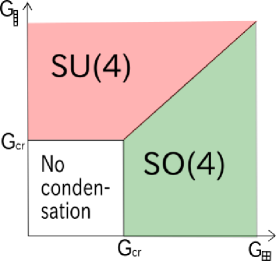
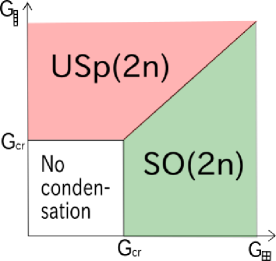
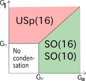
Figure 2: Even $N=2n\geq 4$: $SU(2n)$ phase diagrams are shown in the coupling constant plane $(G_{{\raisebox{-1.5pt}{\rule{3.0pt}{0.4pt}\hskip-3.0pt\rule{0.4pt}{3.0pt}\hskip 3.0pt\hskip-0.4pt\hskip-3.0pt\rule[3.0pt]{3.0pt}{0.4pt}\rule[3.0pt]{0.4pt}{0.4pt}\hskip-0.4pt\rule{0.4pt}{3.0pt}\hskip-0.4pt\rule{3.0pt}{0.4pt}\hskip-3.0pt\rule{0.4pt}{3.0pt}\hskip 3.0pt\hskip-0.4pt\hskip-3.0pt\rule[3.0pt]{3.0pt}{0.4pt}\rule[3.0pt]{0.4pt}{0.4pt}\hskip-0.4pt\rule{0.4pt}{3.0pt}\hskip-0.4pt}\hskip-6.0pt\raisebox{1.5pt}{\rule{3.0pt}{0.4pt}\hskip-3.0pt\rule{0.4pt}{3.0pt}\hskip 3.0pt\hskip-0.4pt\hskip-3.0pt\rule[3.0pt]{3.0pt}{0.4pt}\rule[3.0pt]{0.4pt}{0.4pt}\hskip-0.4pt\rule{0.4pt}{3.0pt}\hskip-0.4pt\rule{3.0pt}{0.4pt}\hskip-3.0pt\rule{0.4pt}{3.0pt}\hskip 3.0pt\hskip-0.4pt\hskip-3.0pt\rule[3.0pt]{3.0pt}{0.4pt}\rule[3.0pt]{0.4pt}{0.4pt}\hskip-0.4pt\rule{0.4pt}{3.0pt}\hskip-0.4pt}}}\,,\ G_{{\raisebox{-3.0pt}{\raisebox{-1.5pt}{\rule{3.0pt}{0.4pt}\hskip-3.0pt\rule{0.4pt}{3.0pt}\hskip 3.0pt\hskip-0.4pt\hskip-3.0pt\rule[3.0pt]{3.0pt}{0.4pt}\rule[3.0pt]{0.4pt}{0.4pt}\hskip-0.4pt\rule{0.4pt}{3.0pt}\hskip-0.4pt}\hskip-3.0pt\raisebox{1.5pt}{\rule{3.0pt}{0.4pt}\hskip-3.0pt\rule{0.4pt}{3.0pt}\hskip 3.0pt\hskip-0.4pt\hskip-3.0pt\rule[3.0pt]{3.0pt}{0.4pt}\rule[3.0pt]{0.4pt}{0.4pt}\hskip-0.4pt\rule{0.4pt}{3.0pt}\hskip-0.4pt}}\hskip-3.0pt\raisebox{3.0pt}{\raisebox{-1.5pt}{\rule{3.0pt}{0.4pt}\hskip-3.0pt\rule{0.4pt}{3.0pt}\hskip 3.0pt\hskip-0.4pt\hskip-3.0pt\rule[3.0pt]{3.0pt}{0.4pt}\rule[3.0pt]{0.4pt}{0.4pt}\hskip-0.4pt\rule{0.4pt}{3.0pt}\hskip-0.4pt}\hskip-3.0pt\raisebox{1.5pt}{\rule{3.0pt}{0.4pt}\hskip-3.0pt\rule{0.4pt}{3.0pt}\hskip 3.0pt\hskip-0.4pt\hskip-3.0pt\rule[3.0pt]{3.0pt}{0.4pt}\rule[3.0pt]{0.4pt}{0.4pt}\hskip-0.4pt\rule{0.4pt}{3.0pt}\hskip-0.4pt}}}})$ for $n=2$ (left figure) and $n\geq 3,\ \not=8$ (middle figure) and $n=8$ (right figure) cases.

Here, however, we should comment on the possibility of further breaking of the $SU(N-4)$ part of $SU(4)\times SU(N-4)$, which exists for $n\geq 3$ and can actually make the potential lower as remarked before. However, in this coupling region, we now know that the breaking $SU(N-4)\to USp(N-4)$ realizes the lowest potential energy, so we should consider the possibility of the successive breaking $SU(N)\to SU(4)\times SU(N-4)\to SU(4)\times USp(N-4)$. But, since the first and second breakings have no interference, we have

$$V_{{SU(4)\times USp(N-4)}}\big{|}_{\text{min}} = V_{{SU(4)\times SU(N-4)}}\big{|}_{\text{min}}+V_{{USp(N-4)}}\big{|}_{\text{min}}.$$ (4.62)

This should be compared with the value $V_{{USp(N=2n)}}\big{|}_{\text{min}}$. Although we do not show an explicit proof here, it is almost evident that

$$V_{{USp(2n)}}\big{|}_{\text{min}}<V_{{SU(4)\times USp(N-4)}}\big{|}_{\text{min}}.$$ (4.63)

This is because the number of the massive fermions on the $USp(2n)$ vacuum is much larger than that on the $SU(4)\times USp(N-4)$ vacuum; the difference is

$$n(2n-1)-\left(6+(n-2)\bigl{(}2(n-2)-1\bigr{)}\right)=8n-16$$ (4.64)

which is larger than 8 already at the lowest value $n=3$ here. So the above conclusion of the $SU(2n)\to USp(2n)$ breaking is still valid even if the possibility of the breaking into non-maximal little groups is taken into account.

Odd $N\geq 3$

From Table 2, for $N=3$, only the case 3) is possible; for $N\geq 5$, the cases 2), 3) and 4) are possible.

Obviously, for $N=3$, $SU(3)$ is broken to the maximal special subgroup $SO(3)$ as far as $G_{{\raisebox{-1.5pt}{\rule{3.0pt}{0.4pt}\hskip-3.0pt\rule{0.4pt}{3.0pt}\hskip 3.0pt\hskip-0.4pt\hskip-3.0pt\rule[3.0pt]{3.0pt}{0.4pt}\rule[3.0pt]{0.4pt}{0.4pt}\hskip-0.4pt\rule{0.4pt}{3.0pt}\hskip-0.4pt\rule{3.0pt}{0.4pt}\hskip-3.0pt\rule{0.4pt}{3.0pt}\hskip 3.0pt\hskip-0.4pt\hskip-3.0pt\rule[3.0pt]{3.0pt}{0.4pt}\rule[3.0pt]{0.4pt}{0.4pt}\hskip-0.4pt\rule{0.4pt}{3.0pt}\hskip-0.4pt}\hskip-6.0pt\raisebox{1.5pt}{\rule{3.0pt}{0.4pt}\hskip-3.0pt\rule{0.4pt}{3.0pt}\hskip 3.0pt\hskip-0.4pt\hskip-3.0pt\rule[3.0pt]{3.0pt}{0.4pt}\rule[3.0pt]{0.4pt}{0.4pt}\hskip-0.4pt\rule{0.4pt}{3.0pt}\hskip-0.4pt\rule{3.0pt}{0.4pt}\hskip-3.0pt\rule{0.4pt}{3.0pt}\hskip 3.0pt\hskip-0.4pt\hskip-3.0pt\rule[3.0pt]{3.0pt}{0.4pt}\rule[3.0pt]{0.4pt}{0.4pt}\hskip-0.4pt\rule{0.4pt}{3.0pt}\hskip-0.4pt}}}$ is larger than its critical coupling. We will discuss the potentials for $N\geq 5$ in detail.

(a) $M^{2}_{{\raisebox{-3.0pt}{\raisebox{-1.5pt}{\rule{3.0pt}{0.4pt}\hskip-3.0pt\rule{0.4pt}{3.0pt}\hskip 3.0pt\hskip-0.4pt\hskip-3.0pt\rule[3.0pt]{3.0pt}{0.4pt}\rule[3.0pt]{0.4pt}{0.4pt}\hskip-0.4pt\rule{0.4pt}{3.0pt}\hskip-0.4pt}\hskip-3.0pt\raisebox{1.5pt}{\rule{3.0pt}{0.4pt}\hskip-3.0pt\rule{0.4pt}{3.0pt}\hskip 3.0pt\hskip-0.4pt\hskip-3.0pt\rule[3.0pt]{3.0pt}{0.4pt}\rule[3.0pt]{0.4pt}{0.4pt}\hskip-0.4pt\rule{0.4pt}{3.0pt}\hskip-0.4pt}}\hskip-3.0pt\raisebox{3.0pt}{\raisebox{-1.5pt}{\rule{3.0pt}{0.4pt}\hskip-3.0pt\rule{0.4pt}{3.0pt}\hskip 3.0pt\hskip-0.4pt\hskip-3.0pt\rule[3.0pt]{3.0pt}{0.4pt}\rule[3.0pt]{0.4pt}{0.4pt}\hskip-0.4pt\rule{0.4pt}{3.0pt}\hskip-0.4pt}\hskip-3.0pt\raisebox{1.5pt}{\rule{3.0pt}{0.4pt}\hskip-3.0pt\rule{0.4pt}{3.0pt}\hskip 3.0pt\hskip-0.4pt\hskip-3.0pt\rule[3.0pt]{3.0pt}{0.4pt}\rule[3.0pt]{0.4pt}{0.4pt}\hskip-0.4pt\rule{0.4pt}{3.0pt}\hskip-0.4pt}}}}>M^{2}_{{\raisebox{-1.5pt}{\rule{3.0pt}{0.4pt}\hskip-3.0pt\rule{0.4pt}{3.0pt}\hskip 3.0pt\hskip-0.4pt\hskip-3.0pt\rule[3.0pt]{3.0pt}{0.4pt}\rule[3.0pt]{0.4pt}{0.4pt}\hskip-0.4pt\rule{0.4pt}{3.0pt}\hskip-0.4pt\rule{3.0pt}{0.4pt}\hskip-3.0pt\rule{0.4pt}{3.0pt}\hskip 3.0pt\hskip-0.4pt\hskip-3.0pt\rule[3.0pt]{3.0pt}{0.4pt}\rule[3.0pt]{0.4pt}{0.4pt}\hskip-0.4pt\rule{0.4pt}{3.0pt}\hskip-0.4pt}\hskip-6.0pt\raisebox{1.5pt}{\rule{3.0pt}{0.4pt}\hskip-3.0pt\rule{0.4pt}{3.0pt}\hskip 3.0pt\hskip-0.4pt\hskip-3.0pt\rule[3.0pt]{3.0pt}{0.4pt}\rule[3.0pt]{0.4pt}{0.4pt}\hskip-0.4pt\rule{0.4pt}{3.0pt}\hskip-0.4pt\rule{3.0pt}{0.4pt}\hskip-3.0pt\rule{0.4pt}{3.0pt}\hskip 3.0pt\hskip-0.4pt\hskip-3.0pt\rule[3.0pt]{3.0pt}{0.4pt}\rule[3.0pt]{0.4pt}{0.4pt}\hskip-0.4pt\rule{0.4pt}{3.0pt}\hskip-0.4pt}}}$ and (b) $M^{2}_{{\raisebox{-3.0pt}{\raisebox{-1.5pt}{\rule{3.0pt}{0.4pt}\hskip-3.0pt\rule{0.4pt}{3.0pt}\hskip 3.0pt\hskip-0.4pt\hskip-3.0pt\rule[3.0pt]{3.0pt}{0.4pt}\rule[3.0pt]{0.4pt}{0.4pt}\hskip-0.4pt\rule{0.4pt}{3.0pt}\hskip-0.4pt}\hskip-3.0pt\raisebox{1.5pt}{\rule{3.0pt}{0.4pt}\hskip-3.0pt\rule{0.4pt}{3.0pt}\hskip 3.0pt\hskip-0.4pt\hskip-3.0pt\rule[3.0pt]{3.0pt}{0.4pt}\rule[3.0pt]{0.4pt}{0.4pt}\hskip-0.4pt\rule{0.4pt}{3.0pt}\hskip-0.4pt}}\hskip-3.0pt\raisebox{3.0pt}{\raisebox{-1.5pt}{\rule{3.0pt}{0.4pt}\hskip-3.0pt\rule{0.4pt}{3.0pt}\hskip 3.0pt\hskip-0.4pt\hskip-3.0pt\rule[3.0pt]{3.0pt}{0.4pt}\rule[3.0pt]{0.4pt}{0.4pt}\hskip-0.4pt\rule{0.4pt}{3.0pt}\hskip-0.4pt}\hskip-3.0pt\raisebox{1.5pt}{\rule{3.0pt}{0.4pt}\hskip-3.0pt\rule{0.4pt}{3.0pt}\hskip 3.0pt\hskip-0.4pt\hskip-3.0pt\rule[3.0pt]{3.0pt}{0.4pt}\rule[3.0pt]{0.4pt}{0.4pt}\hskip-0.4pt\rule{0.4pt}{3.0pt}\hskip-0.4pt}}}}=M^{2}_{{\raisebox{-1.5pt}{\rule{3.0pt}{0.4pt}\hskip-3.0pt\rule{0.4pt}{3.0pt}\hskip 3.0pt\hskip-0.4pt\hskip-3.0pt\rule[3.0pt]{3.0pt}{0.4pt}\rule[3.0pt]{0.4pt}{0.4pt}\hskip-0.4pt\rule{0.4pt}{3.0pt}\hskip-0.4pt\rule{3.0pt}{0.4pt}\hskip-3.0pt\rule{0.4pt}{3.0pt}\hskip 3.0pt\hskip-0.4pt\hskip-3.0pt\rule[3.0pt]{3.0pt}{0.4pt}\rule[3.0pt]{0.4pt}{0.4pt}\hskip-0.4pt\rule{0.4pt}{3.0pt}\hskip-0.4pt}\hskip-6.0pt\raisebox{1.5pt}{\rule{3.0pt}{0.4pt}\hskip-3.0pt\rule{0.4pt}{3.0pt}\hskip 3.0pt\hskip-0.4pt\hskip-3.0pt\rule[3.0pt]{3.0pt}{0.4pt}\rule[3.0pt]{0.4pt}{0.4pt}\hskip-0.4pt\rule{0.4pt}{3.0pt}\hskip-0.4pt\rule{3.0pt}{0.4pt}\hskip-3.0pt\rule{0.4pt}{3.0pt}\hskip 3.0pt\hskip-0.4pt\hskip-3.0pt\rule[3.0pt]{3.0pt}{0.4pt}\rule[3.0pt]{0.4pt}{0.4pt}\hskip-0.4pt\rule{0.4pt}{3.0pt}\hskip-0.4pt}}}$ cases

We first compare the potentials for cases 2) $SU(4)\times SU(N-4)$ $(N\geq 5)$ and 3) $SO(N=2n+1)$. The inequality in Eq. (4.25) holds also for odd $N\geq 5$. Therefore, we find for $N=2n+1\geq 5$

$$V_{{SU(4)\times SU(N-4)}}\big{|}_{\text{min}}>V_{{SO(N=2n+1)}}\big{|}_{\text{min}}.$$ (4.65)

Next, we compare the potentials for cases 3) $SO(N=2n+1)$ and 4) $USp(N^{\prime}=2n)$ $(N\geq 5)$. From Eq. (4.28) for (a) $M^{2}_{{\raisebox{-3.0pt}{\raisebox{-1.5pt}{\rule{3.0pt}{0.4pt}\hskip-3.0pt\rule{0.4pt}{3.0pt}\hskip 3.0pt\hskip-0.4pt\hskip-3.0pt\rule[3.0pt]{3.0pt}{0.4pt}\rule[3.0pt]{0.4pt}{0.4pt}\hskip-0.4pt\rule{0.4pt}{3.0pt}\hskip-0.4pt}\hskip-3.0pt\raisebox{1.5pt}{\rule{3.0pt}{0.4pt}\hskip-3.0pt\rule{0.4pt}{3.0pt}\hskip 3.0pt\hskip-0.4pt\hskip-3.0pt\rule[3.0pt]{3.0pt}{0.4pt}\rule[3.0pt]{0.4pt}{0.4pt}\hskip-0.4pt\rule{0.4pt}{3.0pt}\hskip-0.4pt}}\hskip-3.0pt\raisebox{3.0pt}{\raisebox{-1.5pt}{\rule{3.0pt}{0.4pt}\hskip-3.0pt\rule{0.4pt}{3.0pt}\hskip 3.0pt\hskip-0.4pt\hskip-3.0pt\rule[3.0pt]{3.0pt}{0.4pt}\rule[3.0pt]{0.4pt}{0.4pt}\hskip-0.4pt\rule{0.4pt}{3.0pt}\hskip-0.4pt}\hskip-3.0pt\raisebox{1.5pt}{\rule{3.0pt}{0.4pt}\hskip-3.0pt\rule{0.4pt}{3.0pt}\hskip 3.0pt\hskip-0.4pt\hskip-3.0pt\rule[3.0pt]{3.0pt}{0.4pt}\rule[3.0pt]{0.4pt}{0.4pt}\hskip-0.4pt\rule{0.4pt}{3.0pt}\hskip-0.4pt}}}}>M^{2}_{{\raisebox{-1.5pt}{\rule{3.0pt}{0.4pt}\hskip-3.0pt\rule{0.4pt}{3.0pt}\hskip 3.0pt\hskip-0.4pt\hskip-3.0pt\rule[3.0pt]{3.0pt}{0.4pt}\rule[3.0pt]{0.4pt}{0.4pt}\hskip-0.4pt\rule{0.4pt}{3.0pt}\hskip-0.4pt\rule{3.0pt}{0.4pt}\hskip-3.0pt\rule{0.4pt}{3.0pt}\hskip 3.0pt\hskip-0.4pt\hskip-3.0pt\rule[3.0pt]{3.0pt}{0.4pt}\rule[3.0pt]{0.4pt}{0.4pt}\hskip-0.4pt\rule{0.4pt}{3.0pt}\hskip-0.4pt}\hskip-6.0pt\raisebox{1.5pt}{\rule{3.0pt}{0.4pt}\hskip-3.0pt\rule{0.4pt}{3.0pt}\hskip 3.0pt\hskip-0.4pt\hskip-3.0pt\rule[3.0pt]{3.0pt}{0.4pt}\rule[3.0pt]{0.4pt}{0.4pt}\hskip-0.4pt\rule{0.4pt}{3.0pt}\hskip-0.4pt\rule{3.0pt}{0.4pt}\hskip-3.0pt\rule{0.4pt}{3.0pt}\hskip 3.0pt\hskip-0.4pt\hskip-3.0pt\rule[3.0pt]{3.0pt}{0.4pt}\rule[3.0pt]{0.4pt}{0.4pt}\hskip-0.4pt\rule{0.4pt}{3.0pt}\hskip-0.4pt}}}$ case and Eq. (4.33) for (b) $M^{2}_{{\raisebox{-3.0pt}{\raisebox{-1.5pt}{\rule{3.0pt}{0.4pt}\hskip-3.0pt\rule{0.4pt}{3.0pt}\hskip 3.0pt\hskip-0.4pt\hskip-3.0pt\rule[3.0pt]{3.0pt}{0.4pt}\rule[3.0pt]{0.4pt}{0.4pt}\hskip-0.4pt\rule{0.4pt}{3.0pt}\hskip-0.4pt}\hskip-3.0pt\raisebox{1.5pt}{\rule{3.0pt}{0.4pt}\hskip-3.0pt\rule{0.4pt}{3.0pt}\hskip 3.0pt\hskip-0.4pt\hskip-3.0pt\rule[3.0pt]{3.0pt}{0.4pt}\rule[3.0pt]{0.4pt}{0.4pt}\hskip-0.4pt\rule{0.4pt}{3.0pt}\hskip-0.4pt}}\hskip-3.0pt\raisebox{3.0pt}{\raisebox{-1.5pt}{\rule{3.0pt}{0.4pt}\hskip-3.0pt\rule{0.4pt}{3.0pt}\hskip 3.0pt\hskip-0.4pt\hskip-3.0pt\rule[3.0pt]{3.0pt}{0.4pt}\rule[3.0pt]{0.4pt}{0.4pt}\hskip-0.4pt\rule{0.4pt}{3.0pt}\hskip-0.4pt}\hskip-3.0pt\raisebox{1.5pt}{\rule{3.0pt}{0.4pt}\hskip-3.0pt\rule{0.4pt}{3.0pt}\hskip 3.0pt\hskip-0.4pt\hskip-3.0pt\rule[3.0pt]{3.0pt}{0.4pt}\rule[3.0pt]{0.4pt}{0.4pt}\hskip-0.4pt\rule{0.4pt}{3.0pt}\hskip-0.4pt}}}}=M^{2}_{{\raisebox{-1.5pt}{\rule{3.0pt}{0.4pt}\hskip-3.0pt\rule{0.4pt}{3.0pt}\hskip 3.0pt\hskip-0.4pt\hskip-3.0pt\rule[3.0pt]{3.0pt}{0.4pt}\rule[3.0pt]{0.4pt}{0.4pt}\hskip-0.4pt\rule{0.4pt}{3.0pt}\hskip-0.4pt\rule{3.0pt}{0.4pt}\hskip-3.0pt\rule{0.4pt}{3.0pt}\hskip 3.0pt\hskip-0.4pt\hskip-3.0pt\rule[3.0pt]{3.0pt}{0.4pt}\rule[3.0pt]{0.4pt}{0.4pt}\hskip-0.4pt\rule{0.4pt}{3.0pt}\hskip-0.4pt}\hskip-6.0pt\raisebox{1.5pt}{\rule{3.0pt}{0.4pt}\hskip-3.0pt\rule{0.4pt}{3.0pt}\hskip 3.0pt\hskip-0.4pt\hskip-3.0pt\rule[3.0pt]{3.0pt}{0.4pt}\rule[3.0pt]{0.4pt}{0.4pt}\hskip-0.4pt\rule{0.4pt}{3.0pt}\hskip-0.4pt\rule{3.0pt}{0.4pt}\hskip-3.0pt\rule{0.4pt}{3.0pt}\hskip 3.0pt\hskip-0.4pt\hskip-3.0pt\rule[3.0pt]{3.0pt}{0.4pt}\rule[3.0pt]{0.4pt}{0.4pt}\hskip-0.4pt\rule{0.4pt}{3.0pt}\hskip-0.4pt}}}$ case, we know

$$V_{{USp(2n)}}(v,V)\big{|}_{\text{min}}\geq \frac{N^{\prime}(N^{\prime}-1)}{2}F(V_{0}^{2};M_{{\raisebox{-1.5pt}{\rule{3.0pt}{0.4pt}\hskip-3.0pt\rule{0.4pt}{3.0pt}\hskip 3.0pt\hskip-0.4pt\hskip-3.0pt\rule[3.0pt]{3.0pt}{0.4pt}\rule[3.0pt]{0.4pt}{0.4pt}\hskip-0.4pt\rule{0.4pt}{3.0pt}\hskip-0.4pt\rule{3.0pt}{0.4pt}\hskip-3.0pt\rule{0.4pt}{3.0pt}\hskip 3.0pt\hskip-0.4pt\hskip-3.0pt\rule[3.0pt]{3.0pt}{0.4pt}\rule[3.0pt]{0.4pt}{0.4pt}\hskip-0.4pt\rule{0.4pt}{3.0pt}\hskip-0.4pt}\hskip-6.0pt\raisebox{1.5pt}{\rule{3.0pt}{0.4pt}\hskip-3.0pt\rule{0.4pt}{3.0pt}\hskip 3.0pt\hskip-0.4pt\hskip-3.0pt\rule[3.0pt]{3.0pt}{0.4pt}\rule[3.0pt]{0.4pt}{0.4pt}\hskip-0.4pt\rule{0.4pt}{3.0pt}\hskip-0.4pt\rule{3.0pt}{0.4pt}\hskip-3.0pt\rule{0.4pt}{3.0pt}\hskip 3.0pt\hskip-0.4pt\hskip-3.0pt\rule[3.0pt]{3.0pt}{0.4pt}\rule[3.0pt]{0.4pt}{0.4pt}\hskip-0.4pt\rule{0.4pt}{3.0pt}\hskip-0.4pt}}}^{2})=V_{{SO(2n)}}\big{|}_{\text{min}}$$ (4.66)

with equality for the case (b). But, since Eq. (4.3) tells us the inequality

$$V_{{SO(2n)}}\big{|}_{\text{min}}>V_{{SO(2n+1)}}\big{|}_{\text{min}},$$ (4.67)

we have anyway

$$V_{{USp(N^{\prime}=2n)}}(v,V)\big{|}_{\text{min}}>V_{{SO(N=2n+1)}}\big{|}_{\text{min}}.$$ (4.68)

Thus, the $SO(N=2n+1)$ $(N\geq 5)$ vacuum realizes the lowest potential value and we can conclude that the symmetry breaking in these cases $M^{2}_{{\raisebox{-3.0pt}{\raisebox{-1.5pt}{\rule{3.0pt}{0.4pt}\hskip-3.0pt\rule{0.4pt}{3.0pt}\hskip 3.0pt\hskip-0.4pt\hskip-3.0pt\rule[3.0pt]{3.0pt}{0.4pt}\rule[3.0pt]{0.4pt}{0.4pt}\hskip-0.4pt\rule{0.4pt}{3.0pt}\hskip-0.4pt}\hskip-3.0pt\raisebox{1.5pt}{\rule{3.0pt}{0.4pt}\hskip-3.0pt\rule{0.4pt}{3.0pt}\hskip 3.0pt\hskip-0.4pt\hskip-3.0pt\rule[3.0pt]{3.0pt}{0.4pt}\rule[3.0pt]{0.4pt}{0.4pt}\hskip-0.4pt\rule{0.4pt}{3.0pt}\hskip-0.4pt}}\hskip-3.0pt\raisebox{3.0pt}{\raisebox{-1.5pt}{\rule{3.0pt}{0.4pt}\hskip-3.0pt\rule{0.4pt}{3.0pt}\hskip 3.0pt\hskip-0.4pt\hskip-3.0pt\rule[3.0pt]{3.0pt}{0.4pt}\rule[3.0pt]{0.4pt}{0.4pt}\hskip-0.4pt\rule{0.4pt}{3.0pt}\hskip-0.4pt}\hskip-3.0pt\raisebox{1.5pt}{\rule{3.0pt}{0.4pt}\hskip-3.0pt\rule{0.4pt}{3.0pt}\hskip 3.0pt\hskip-0.4pt\hskip-3.0pt\rule[3.0pt]{3.0pt}{0.4pt}\rule[3.0pt]{0.4pt}{0.4pt}\hskip-0.4pt\rule{0.4pt}{3.0pt}\hskip-0.4pt}}}}{\geq}M^{2}_{{\raisebox{-1.5pt}{\rule{3.0pt}{0.4pt}\hskip-3.0pt\rule{0.4pt}{3.0pt}\hskip 3.0pt\hskip-0.4pt\hskip-3.0pt\rule[3.0pt]{3.0pt}{0.4pt}\rule[3.0pt]{0.4pt}{0.4pt}\hskip-0.4pt\rule{0.4pt}{3.0pt}\hskip-0.4pt\rule{3.0pt}{0.4pt}\hskip-3.0pt\rule{0.4pt}{3.0pt}\hskip 3.0pt\hskip-0.4pt\hskip-3.0pt\rule[3.0pt]{3.0pt}{0.4pt}\rule[3.0pt]{0.4pt}{0.4pt}\hskip-0.4pt\rule{0.4pt}{3.0pt}\hskip-0.4pt}\hskip-6.0pt\raisebox{1.5pt}{\rule{3.0pt}{0.4pt}\hskip-3.0pt\rule{0.4pt}{3.0pt}\hskip 3.0pt\hskip-0.4pt\hskip-3.0pt\rule[3.0pt]{3.0pt}{0.4pt}\rule[3.0pt]{0.4pt}{0.4pt}\hskip-0.4pt\rule{0.4pt}{3.0pt}\hskip-0.4pt\rule{3.0pt}{0.4pt}\hskip-3.0pt\rule{0.4pt}{3.0pt}\hskip 3.0pt\hskip-0.4pt\hskip-3.0pt\rule[3.0pt]{3.0pt}{0.4pt}\rule[3.0pt]{0.4pt}{0.4pt}\hskip-0.4pt\rule{0.4pt}{3.0pt}\hskip-0.4pt}}}$ is also a breaking to special subgroup:

$$SU(N=2n+1)\quad\rightarrow\quad SO(N=2n+1)\ .$$ (4.69)

(c) $M^{2}_{{\raisebox{-3.0pt}{\raisebox{-1.5pt}{\rule{3.0pt}{0.4pt}\hskip-3.0pt\rule{0.4pt}{3.0pt}\hskip 3.0pt\hskip-0.4pt\hskip-3.0pt\rule[3.0pt]{3.0pt}{0.4pt}\rule[3.0pt]{0.4pt}{0.4pt}\hskip-0.4pt\rule{0.4pt}{3.0pt}\hskip-0.4pt}\hskip-3.0pt\raisebox{1.5pt}{\rule{3.0pt}{0.4pt}\hskip-3.0pt\rule{0.4pt}{3.0pt}\hskip 3.0pt\hskip-0.4pt\hskip-3.0pt\rule[3.0pt]{3.0pt}{0.4pt}\rule[3.0pt]{0.4pt}{0.4pt}\hskip-0.4pt\rule{0.4pt}{3.0pt}\hskip-0.4pt}}\hskip-3.0pt\raisebox{3.0pt}{\raisebox{-1.5pt}{\rule{3.0pt}{0.4pt}\hskip-3.0pt\rule{0.4pt}{3.0pt}\hskip 3.0pt\hskip-0.4pt\hskip-3.0pt\rule[3.0pt]{3.0pt}{0.4pt}\rule[3.0pt]{0.4pt}{0.4pt}\hskip-0.4pt\rule{0.4pt}{3.0pt}\hskip-0.4pt}\hskip-3.0pt\raisebox{1.5pt}{\rule{3.0pt}{0.4pt}\hskip-3.0pt\rule{0.4pt}{3.0pt}\hskip 3.0pt\hskip-0.4pt\hskip-3.0pt\rule[3.0pt]{3.0pt}{0.4pt}\rule[3.0pt]{0.4pt}{0.4pt}\hskip-0.4pt\rule{0.4pt}{3.0pt}\hskip-0.4pt}}}}<M^{2}_{{\raisebox{-1.5pt}{\rule{3.0pt}{0.4pt}\hskip-3.0pt\rule{0.4pt}{3.0pt}\hskip 3.0pt\hskip-0.4pt\hskip-3.0pt\rule[3.0pt]{3.0pt}{0.4pt}\rule[3.0pt]{0.4pt}{0.4pt}\hskip-0.4pt\rule{0.4pt}{3.0pt}\hskip-0.4pt\rule{3.0pt}{0.4pt}\hskip-3.0pt\rule{0.4pt}{3.0pt}\hskip 3.0pt\hskip-0.4pt\hskip-3.0pt\rule[3.0pt]{3.0pt}{0.4pt}\rule[3.0pt]{0.4pt}{0.4pt}\hskip-0.4pt\rule{0.4pt}{3.0pt}\hskip-0.4pt}\hskip-6.0pt\raisebox{1.5pt}{\rule{3.0pt}{0.4pt}\hskip-3.0pt\rule{0.4pt}{3.0pt}\hskip 3.0pt\hskip-0.4pt\hskip-3.0pt\rule[3.0pt]{3.0pt}{0.4pt}\rule[3.0pt]{0.4pt}{0.4pt}\hskip-0.4pt\rule{0.4pt}{3.0pt}\hskip-0.4pt\rule{3.0pt}{0.4pt}\hskip-3.0pt\rule{0.4pt}{3.0pt}\hskip 3.0pt\hskip-0.4pt\hskip-3.0pt\rule[3.0pt]{3.0pt}{0.4pt}\rule[3.0pt]{0.4pt}{0.4pt}\hskip-0.4pt\rule{0.4pt}{3.0pt}\hskip-0.4pt}}}$ case

In this coupling region, the condensation into $\Phi_{\raisebox{-3.0pt}{\raisebox{-1.5pt}{\rule{3.0pt}{0.4pt}\hskip-3.0pt\rule{0.4pt}{3.0pt}\hskip 3.0pt\hskip-0.4pt\hskip-3.0pt\rule[3.0pt]{3.0pt}{0.4pt}\rule[3.0pt]{0.4pt}{0.4pt}\hskip-0.4pt\rule{0.4pt}{3.0pt}\hskip-0.4pt}\hskip-3.0pt\raisebox{1.5pt}{\rule{3.0pt}{0.4pt}\hskip-3.0pt\rule{0.4pt}{3.0pt}\hskip 3.0pt\hskip-0.4pt\hskip-3.0pt\rule[3.0pt]{3.0pt}{0.4pt}\rule[3.0pt]{0.4pt}{0.4pt}\hskip-0.4pt\rule{0.4pt}{3.0pt}\hskip-0.4pt}}\hskip-3.0pt\raisebox{3.0pt}{\raisebox{-1.5pt}{\rule{3.0pt}{0.4pt}\hskip-3.0pt\rule{0.4pt}{3.0pt}\hskip 3.0pt\hskip-0.4pt\hskip-3.0pt\rule[3.0pt]{3.0pt}{0.4pt}\rule[3.0pt]{0.4pt}{0.4pt}\hskip-0.4pt\rule{0.4pt}{3.0pt}\hskip-0.4pt}\hskip-3.0pt\raisebox{1.5pt}{\rule{3.0pt}{0.4pt}\hskip-3.0pt\rule{0.4pt}{3.0pt}\hskip 3.0pt\hskip-0.4pt\hskip-3.0pt\rule[3.0pt]{3.0pt}{0.4pt}\rule[3.0pt]{0.4pt}{0.4pt}\hskip-0.4pt\rule{0.4pt}{3.0pt}\hskip-0.4pt}}}$ is preferred to into $\Phi_{\raisebox{-1.5pt}{\rule{3.0pt}{0.4pt}\hskip-3.0pt\rule{0.4pt}{3.0pt}\hskip 3.0pt\hskip-0.4pt\hskip-3.0pt\rule[3.0pt]{3.0pt}{0.4pt}\rule[3.0pt]{0.4pt}{0.4pt}\hskip-0.4pt\rule{0.4pt}{3.0pt}\hskip-0.4pt\rule{3.0pt}{0.4pt}\hskip-3.0pt\rule{0.4pt}{3.0pt}\hskip 3.0pt\hskip-0.4pt\hskip-3.0pt\rule[3.0pt]{3.0pt}{0.4pt}\rule[3.0pt]{0.4pt}{0.4pt}\hskip-0.4pt\rule{0.4pt}{3.0pt}\hskip-0.4pt}\hskip-6.0pt\raisebox{1.5pt}{\rule{3.0pt}{0.4pt}\hskip-3.0pt\rule{0.4pt}{3.0pt}\hskip 3.0pt\hskip-0.4pt\hskip-3.0pt\rule[3.0pt]{3.0pt}{0.4pt}\rule[3.0pt]{0.4pt}{0.4pt}\hskip-0.4pt\rule{0.4pt}{3.0pt}\hskip-0.4pt\rule{3.0pt}{0.4pt}\hskip-3.0pt\rule{0.4pt}{3.0pt}\hskip 3.0pt\hskip-0.4pt\hskip-3.0pt\rule[3.0pt]{3.0pt}{0.4pt}\rule[3.0pt]{0.4pt}{0.4pt}\hskip-0.4pt\rule{0.4pt}{3.0pt}\hskip-0.4pt}}$. Here we first compare the potentials for 2) $SU(4)\times SU(N-4)$ and 4) $USp(N^{\prime}=N-1)$ for $(N\geq 5)$. The same discussion as in even $N$, given from Eq. (4.39) to Eq. (4.60), holds if $n\geq 3$, so that we have, for $N=2n+1\geq 7$,

$$V_{{USp(N^{\prime}=2n)}}|_{\text{min}}<V_{{SU(4)\times SU(N-4)}}|_{\text{min}}.$$ (4.70)

For $N=5$, however, $USp(N^{\prime}=4)$ is not the maximal little group of                                  , for which the $SU(4)\times SU(N-4)=SU(4)$ is the maximal little group. Since six fermions of $SU(4)$ 6 all can get a common mass square realizing the minimum of the potential $F(v^{2};M_{{\raisebox{-3.0pt}{\raisebox{-1.5pt}{\rule{3.0pt}{0.4pt}\hskip-3.0pt\rule{0.4pt}{3.0pt}\hskip 3.0pt\hskip-0.4pt\hskip-3.0pt\rule[3.0pt]{3.0pt}{0.4pt}\rule[3.0pt]{0.4pt}{0.4pt}\hskip-0.4pt\rule{0.4pt}{3.0pt}\hskip-0.4pt}\hskip-3.0pt\raisebox{1.5pt}{\rule{3.0pt}{0.4pt}\hskip-3.0pt\rule{0.4pt}{3.0pt}\hskip 3.0pt\hskip-0.4pt\hskip-3.0pt\rule[3.0pt]{3.0pt}{0.4pt}\rule[3.0pt]{0.4pt}{0.4pt}\hskip-0.4pt\rule{0.4pt}{3.0pt}\hskip-0.4pt}}\hskip-3.0pt\raisebox{3.0pt}{\raisebox{-1.5pt}{\rule{3.0pt}{0.4pt}\hskip-3.0pt\rule{0.4pt}{3.0pt}\hskip 3.0pt\hskip-0.4pt\hskip-3.0pt\rule[3.0pt]{3.0pt}{0.4pt}\rule[3.0pt]{0.4pt}{0.4pt}\hskip-0.4pt\rule{0.4pt}{3.0pt}\hskip-0.4pt}\hskip-3.0pt\raisebox{1.5pt}{\rule{3.0pt}{0.4pt}\hskip-3.0pt\rule{0.4pt}{3.0pt}\hskip 3.0pt\hskip-0.4pt\hskip-3.0pt\rule[3.0pt]{3.0pt}{0.4pt}\rule[3.0pt]{0.4pt}{0.4pt}\hskip-0.4pt\rule{0.4pt}{3.0pt}\hskip-0.4pt}}}}^{2})$ for the $SU(4)$ vacuum case, while they must split into ${\bf 5}+{\bf 1}$ under the subgroup $USp(4)\subset SU(4)$ so leading necessarily to the higher energy than the $SU(4)$ case,

$$V_{{SU(4)}}\big{|}_{\text{min}}<V_{{USp(4)}}\big{|}_{\text{min}}.$$ (4.71)

This is the same inequality as the first part of Eq. (4.38).

Next, we compare the potentials for 3) $SO(N)$ and 2) $SU(4)\times SU(N-4)$ for $N=5$; 4) $USp(N^{\prime}=N-1)$ for $N\geq 7$. If $M_{{\raisebox{-3.0pt}{\raisebox{-1.5pt}{\rule{3.0pt}{0.4pt}\hskip-3.0pt\rule{0.4pt}{3.0pt}\hskip 3.0pt\hskip-0.4pt\hskip-3.0pt\rule[3.0pt]{3.0pt}{0.4pt}\rule[3.0pt]{0.4pt}{0.4pt}\hskip-0.4pt\rule{0.4pt}{3.0pt}\hskip-0.4pt}\hskip-3.0pt\raisebox{1.5pt}{\rule{3.0pt}{0.4pt}\hskip-3.0pt\rule{0.4pt}{3.0pt}\hskip 3.0pt\hskip-0.4pt\hskip-3.0pt\rule[3.0pt]{3.0pt}{0.4pt}\rule[3.0pt]{0.4pt}{0.4pt}\hskip-0.4pt\rule{0.4pt}{3.0pt}\hskip-0.4pt}}\hskip-3.0pt\raisebox{3.0pt}{\raisebox{-1.5pt}{\rule{3.0pt}{0.4pt}\hskip-3.0pt\rule{0.4pt}{3.0pt}\hskip 3.0pt\hskip-0.4pt\hskip-3.0pt\rule[3.0pt]{3.0pt}{0.4pt}\rule[3.0pt]{0.4pt}{0.4pt}\hskip-0.4pt\rule{0.4pt}{3.0pt}\hskip-0.4pt}\hskip-3.0pt\raisebox{1.5pt}{\rule{3.0pt}{0.4pt}\hskip-3.0pt\rule{0.4pt}{3.0pt}\hskip 3.0pt\hskip-0.4pt\hskip-3.0pt\rule[3.0pt]{3.0pt}{0.4pt}\rule[3.0pt]{0.4pt}{0.4pt}\hskip-0.4pt\rule{0.4pt}{3.0pt}\hskip-0.4pt}}}}^{2}$ becomes much smaller than $M_{{\raisebox{-1.5pt}{\rule{3.0pt}{0.4pt}\hskip-3.0pt\rule{0.4pt}{3.0pt}\hskip 3.0pt\hskip-0.4pt\hskip-3.0pt\rule[3.0pt]{3.0pt}{0.4pt}\rule[3.0pt]{0.4pt}{0.4pt}\hskip-0.4pt\rule{0.4pt}{3.0pt}\hskip-0.4pt\rule{3.0pt}{0.4pt}\hskip-3.0pt\rule{0.4pt}{3.0pt}\hskip 3.0pt\hskip-0.4pt\hskip-3.0pt\rule[3.0pt]{3.0pt}{0.4pt}\rule[3.0pt]{0.4pt}{0.4pt}\hskip-0.4pt\rule{0.4pt}{3.0pt}\hskip-0.4pt}\hskip-6.0pt\raisebox{1.5pt}{\rule{3.0pt}{0.4pt}\hskip-3.0pt\rule{0.4pt}{3.0pt}\hskip 3.0pt\hskip-0.4pt\hskip-3.0pt\rule[3.0pt]{3.0pt}{0.4pt}\rule[3.0pt]{0.4pt}{0.4pt}\hskip-0.4pt\rule{0.4pt}{3.0pt}\hskip-0.4pt\rule{3.0pt}{0.4pt}\hskip-3.0pt\rule{0.4pt}{3.0pt}\hskip 3.0pt\hskip-0.4pt\hskip-3.0pt\rule[3.0pt]{3.0pt}{0.4pt}\rule[3.0pt]{0.4pt}{0.4pt}\hskip-0.4pt\rule{0.4pt}{3.0pt}\hskip-0.4pt}}}^{2}$ , i.e., the coupling $G_{{\raisebox{-3.0pt}{\raisebox{-1.5pt}{\rule{3.0pt}{0.4pt}\hskip-3.0pt\rule{0.4pt}{3.0pt}\hskip 3.0pt\hskip-0.4pt\hskip-3.0pt\rule[3.0pt]{3.0pt}{0.4pt}\rule[3.0pt]{0.4pt}{0.4pt}\hskip-0.4pt\rule{0.4pt}{3.0pt}\hskip-0.4pt}\hskip-3.0pt\raisebox{1.5pt}{\rule{3.0pt}{0.4pt}\hskip-3.0pt\rule{0.4pt}{3.0pt}\hskip 3.0pt\hskip-0.4pt\hskip-3.0pt\rule[3.0pt]{3.0pt}{0.4pt}\rule[3.0pt]{0.4pt}{0.4pt}\hskip-0.4pt\rule{0.4pt}{3.0pt}\hskip-0.4pt}}\hskip-3.0pt\raisebox{3.0pt}{\raisebox{-1.5pt}{\rule{3.0pt}{0.4pt}\hskip-3.0pt\rule{0.4pt}{3.0pt}\hskip 3.0pt\hskip-0.4pt\hskip-3.0pt\rule[3.0pt]{3.0pt}{0.4pt}\rule[3.0pt]{0.4pt}{0.4pt}\hskip-0.4pt\rule{0.4pt}{3.0pt}\hskip-0.4pt}\hskip-3.0pt\raisebox{1.5pt}{\rule{3.0pt}{0.4pt}\hskip-3.0pt\rule{0.4pt}{3.0pt}\hskip 3.0pt\hskip-0.4pt\hskip-3.0pt\rule[3.0pt]{3.0pt}{0.4pt}\rule[3.0pt]{0.4pt}{0.4pt}\hskip-0.4pt\rule{0.4pt}{3.0pt}\hskip-0.4pt}}}}$ becomes much stronger than $G_{{\raisebox{-1.5pt}{\rule{3.0pt}{0.4pt}\hskip-3.0pt\rule{0.4pt}{3.0pt}\hskip 3.0pt\hskip-0.4pt\hskip-3.0pt\rule[3.0pt]{3.0pt}{0.4pt}\rule[3.0pt]{0.4pt}{0.4pt}\hskip-0.4pt\rule{0.4pt}{3.0pt}\hskip-0.4pt\rule{3.0pt}{0.4pt}\hskip-3.0pt\rule{0.4pt}{3.0pt}\hskip 3.0pt\hskip-0.4pt\hskip-3.0pt\rule[3.0pt]{3.0pt}{0.4pt}\rule[3.0pt]{0.4pt}{0.4pt}\hskip-0.4pt\rule{0.4pt}{3.0pt}\hskip-0.4pt}\hskip-6.0pt\raisebox{1.5pt}{\rule{3.0pt}{0.4pt}\hskip-3.0pt\rule{0.4pt}{3.0pt}\hskip 3.0pt\hskip-0.4pt\hskip-3.0pt\rule[3.0pt]{3.0pt}{0.4pt}\rule[3.0pt]{0.4pt}{0.4pt}\hskip-0.4pt\rule{0.4pt}{3.0pt}\hskip-0.4pt\rule{3.0pt}{0.4pt}\hskip-3.0pt\rule{0.4pt}{3.0pt}\hskip 3.0pt\hskip-0.4pt\hskip-3.0pt\rule[3.0pt]{3.0pt}{0.4pt}\rule[3.0pt]{0.4pt}{0.4pt}\hskip-0.4pt\rule{0.4pt}{3.0pt}\hskip-0.4pt}}}$ , then the minimum value $F(v_{0}^{2};M_{{\raisebox{-3.0pt}{\raisebox{-1.5pt}{\rule{3.0pt}{0.4pt}\hskip-3.0pt\rule{0.4pt}{3.0pt}\hskip 3.0pt\hskip-0.4pt\hskip-3.0pt\rule[3.0pt]{3.0pt}{0.4pt}\rule[3.0pt]{0.4pt}{0.4pt}\hskip-0.4pt\rule{0.4pt}{3.0pt}\hskip-0.4pt}\hskip-3.0pt\raisebox{1.5pt}{\rule{3.0pt}{0.4pt}\hskip-3.0pt\rule{0.4pt}{3.0pt}\hskip 3.0pt\hskip-0.4pt\hskip-3.0pt\rule[3.0pt]{3.0pt}{0.4pt}\rule[3.0pt]{0.4pt}{0.4pt}\hskip-0.4pt\rule{0.4pt}{3.0pt}\hskip-0.4pt}}\hskip-3.0pt\raisebox{3.0pt}{\raisebox{-1.5pt}{\rule{3.0pt}{0.4pt}\hskip-3.0pt\rule{0.4pt}{3.0pt}\hskip 3.0pt\hskip-0.4pt\hskip-3.0pt\rule[3.0pt]{3.0pt}{0.4pt}\rule[3.0pt]{0.4pt}{0.4pt}\hskip-0.4pt\rule{0.4pt}{3.0pt}\hskip-0.4pt}\hskip-3.0pt\raisebox{1.5pt}{\rule{3.0pt}{0.4pt}\hskip-3.0pt\rule{0.4pt}{3.0pt}\hskip 3.0pt\hskip-0.4pt\hskip-3.0pt\rule[3.0pt]{3.0pt}{0.4pt}\rule[3.0pt]{0.4pt}{0.4pt}\hskip-0.4pt\rule{0.4pt}{3.0pt}\hskip-0.4pt}}}})$ becomes much lower than the minimum value $F(V_{0}^{2};M_{{\raisebox{-1.5pt}{\rule{3.0pt}{0.4pt}\hskip-3.0pt\rule{0.4pt}{3.0pt}\hskip 3.0pt\hskip-0.4pt\hskip-3.0pt\rule[3.0pt]{3.0pt}{0.4pt}\rule[3.0pt]{0.4pt}{0.4pt}\hskip-0.4pt\rule{0.4pt}{3.0pt}\hskip-0.4pt\rule{3.0pt}{0.4pt}\hskip-3.0pt\rule{0.4pt}{3.0pt}\hskip 3.0pt\hskip-0.4pt\hskip-3.0pt\rule[3.0pt]{3.0pt}{0.4pt}\rule[3.0pt]{0.4pt}{0.4pt}\hskip-0.4pt\rule{0.4pt}{3.0pt}\hskip-0.4pt}\hskip-6.0pt\raisebox{1.5pt}{\rule{3.0pt}{0.4pt}\hskip-3.0pt\rule{0.4pt}{3.0pt}\hskip 3.0pt\hskip-0.4pt\hskip-3.0pt\rule[3.0pt]{3.0pt}{0.4pt}\rule[3.0pt]{0.4pt}{0.4pt}\hskip-0.4pt\rule{0.4pt}{3.0pt}\hskip-0.4pt\rule{3.0pt}{0.4pt}\hskip-3.0pt\rule{0.4pt}{3.0pt}\hskip 3.0pt\hskip-0.4pt\hskip-3.0pt\rule[3.0pt]{3.0pt}{0.4pt}\rule[3.0pt]{0.4pt}{0.4pt}\hskip-0.4pt\rule{0.4pt}{3.0pt}\hskip-0.4pt}}})$. The minimum value of the $SU(4)\times SU(N-4)$ potential $V_{{SU(4)\times SU(N-4)}}|_{\text{min}}=6F(v_{0}^{2};M_{{\raisebox{-3.0pt}{\raisebox{-1.5pt}{\rule{3.0pt}{0.4pt}\hskip-3.0pt\rule{0.4pt}{3.0pt}\hskip 3.0pt\hskip-0.4pt\hskip-3.0pt\rule[3.0pt]{3.0pt}{0.4pt}\rule[3.0pt]{0.4pt}{0.4pt}\hskip-0.4pt\rule{0.4pt}{3.0pt}\hskip-0.4pt}\hskip-3.0pt\raisebox{1.5pt}{\rule{3.0pt}{0.4pt}\hskip-3.0pt\rule{0.4pt}{3.0pt}\hskip 3.0pt\hskip-0.4pt\hskip-3.0pt\rule[3.0pt]{3.0pt}{0.4pt}\rule[3.0pt]{0.4pt}{0.4pt}\hskip-0.4pt\rule{0.4pt}{3.0pt}\hskip-0.4pt}}\hskip-3.0pt\raisebox{3.0pt}{\raisebox{-1.5pt}{\rule{3.0pt}{0.4pt}\hskip-3.0pt\rule{0.4pt}{3.0pt}\hskip 3.0pt\hskip-0.4pt\hskip-3.0pt\rule[3.0pt]{3.0pt}{0.4pt}\rule[3.0pt]{0.4pt}{0.4pt}\hskip-0.4pt\rule{0.4pt}{3.0pt}\hskip-0.4pt}\hskip-3.0pt\raisebox{1.5pt}{\rule{3.0pt}{0.4pt}\hskip-3.0pt\rule{0.4pt}{3.0pt}\hskip 3.0pt\hskip-0.4pt\hskip-3.0pt\rule[3.0pt]{3.0pt}{0.4pt}\rule[3.0pt]{0.4pt}{0.4pt}\hskip-0.4pt\rule{0.4pt}{3.0pt}\hskip-0.4pt}}}}^{2})$ or the $USp(N^{\prime}=N-1)$ potential $V_{{USp(N^{\prime}=N-1)}}|_{\text{min}}$, for which the number of the massive fermions is smaller than that for the $SO(N)$ case, can become lower than the minimum value of the $SO(N)$ potential $V_{{SO(N)}}|_{\text{min}}=(N(N-1)/2)F(V_{0}^{2};M_{{\raisebox{-1.5pt}{\rule{3.0pt}{0.4pt}\hskip-3.0pt\rule{0.4pt}{3.0pt}\hskip 3.0pt\hskip-0.4pt\hskip-3.0pt\rule[3.0pt]{3.0pt}{0.4pt}\rule[3.0pt]{0.4pt}{0.4pt}\hskip-0.4pt\rule{0.4pt}{3.0pt}\hskip-0.4pt\rule{3.0pt}{0.4pt}\hskip-3.0pt\rule{0.4pt}{3.0pt}\hskip 3.0pt\hskip-0.4pt\hskip-3.0pt\rule[3.0pt]{3.0pt}{0.4pt}\rule[3.0pt]{0.4pt}{0.4pt}\hskip-0.4pt\rule{0.4pt}{3.0pt}\hskip-0.4pt}\hskip-6.0pt\raisebox{1.5pt}{\rule{3.0pt}{0.4pt}\hskip-3.0pt\rule{0.4pt}{3.0pt}\hskip 3.0pt\hskip-0.4pt\hskip-3.0pt\rule[3.0pt]{3.0pt}{0.4pt}\rule[3.0pt]{0.4pt}{0.4pt}\hskip-0.4pt\rule{0.4pt}{3.0pt}\hskip-0.4pt\rule{3.0pt}{0.4pt}\hskip-3.0pt\rule{0.4pt}{3.0pt}\hskip 3.0pt\hskip-0.4pt\hskip-3.0pt\rule[3.0pt]{3.0pt}{0.4pt}\rule[3.0pt]{0.4pt}{0.4pt}\hskip-0.4pt\rule{0.4pt}{3.0pt}\hskip-0.4pt}}})$ for $N\geq 5$. Thus, we conclude that, for odd $N\geq 5$, the symmetry breaking pattern depends on whether $M_{{\raisebox{-3.0pt}{\raisebox{-1.5pt}{\rule{3.0pt}{0.4pt}\hskip-3.0pt\rule{0.4pt}{3.0pt}\hskip 3.0pt\hskip-0.4pt\hskip-3.0pt\rule[3.0pt]{3.0pt}{0.4pt}\rule[3.0pt]{0.4pt}{0.4pt}\hskip-0.4pt\rule{0.4pt}{3.0pt}\hskip-0.4pt}\hskip-3.0pt\raisebox{1.5pt}{\rule{3.0pt}{0.4pt}\hskip-3.0pt\rule{0.4pt}{3.0pt}\hskip 3.0pt\hskip-0.4pt\hskip-3.0pt\rule[3.0pt]{3.0pt}{0.4pt}\rule[3.0pt]{0.4pt}{0.4pt}\hskip-0.4pt\rule{0.4pt}{3.0pt}\hskip-0.4pt}}\hskip-3.0pt\raisebox{3.0pt}{\raisebox{-1.5pt}{\rule{3.0pt}{0.4pt}\hskip-3.0pt\rule{0.4pt}{3.0pt}\hskip 3.0pt\hskip-0.4pt\hskip-3.0pt\rule[3.0pt]{3.0pt}{0.4pt}\rule[3.0pt]{0.4pt}{0.4pt}\hskip-0.4pt\rule{0.4pt}{3.0pt}\hskip-0.4pt}\hskip-3.0pt\raisebox{1.5pt}{\rule{3.0pt}{0.4pt}\hskip-3.0pt\rule{0.4pt}{3.0pt}\hskip 3.0pt\hskip-0.4pt\hskip-3.0pt\rule[3.0pt]{3.0pt}{0.4pt}\rule[3.0pt]{0.4pt}{0.4pt}\hskip-0.4pt\rule{0.4pt}{3.0pt}\hskip-0.4pt}}}}^{2}$ is larger or smaller than a certain value $M_{0}^{2}$ which depends on $N$: for $N=5$

$$SU(5)\quad\rightarrow\quad\begin{cases}SO(5)&\hbox{for }\exists M_{0}^{2}\leq M_{{\raisebox{-3.0pt}{\raisebox{-1.5pt}{\rule{3.0pt}{0.4pt}\hskip-3.0pt\rule{0.4pt}{3.0pt}\hskip 3.0pt\hskip-0.4pt\hskip-3.0pt\rule[3.0pt]{3.0pt}{0.4pt}\rule[3.0pt]{0.4pt}{0.4pt}\hskip-0.4pt\rule{0.4pt}{3.0pt}\hskip-0.4pt}\hskip-3.0pt\raisebox{1.5pt}{\rule{3.0pt}{0.4pt}\hskip-3.0pt\rule{0.4pt}{3.0pt}\hskip 3.0pt\hskip-0.4pt\hskip-3.0pt\rule[3.0pt]{3.0pt}{0.4pt}\rule[3.0pt]{0.4pt}{0.4pt}\hskip-0.4pt\rule{0.4pt}{3.0pt}\hskip-0.4pt}}\hskip-3.0pt\raisebox{3.0pt}{\raisebox{-1.5pt}{\rule{3.0pt}{0.4pt}\hskip-3.0pt\rule{0.4pt}{3.0pt}\hskip 3.0pt\hskip-0.4pt\hskip-3.0pt\rule[3.0pt]{3.0pt}{0.4pt}\rule[3.0pt]{0.4pt}{0.4pt}\hskip-0.4pt\rule{0.4pt}{3.0pt}\hskip-0.4pt}\hskip-3.0pt\raisebox{1.5pt}{\rule{3.0pt}{0.4pt}\hskip-3.0pt\rule{0.4pt}{3.0pt}\hskip 3.0pt\hskip-0.4pt\hskip-3.0pt\rule[3.0pt]{3.0pt}{0.4pt}\rule[3.0pt]{0.4pt}{0.4pt}\hskip-0.4pt\rule{0.4pt}{3.0pt}\hskip-0.4pt}}}}^{2}\leq M_{{\raisebox{-1.5pt}{\rule{3.0pt}{0.4pt}\hskip-3.0pt\rule{0.4pt}{3.0pt}\hskip 3.0pt\hskip-0.4pt\hskip-3.0pt\rule[3.0pt]{3.0pt}{0.4pt}\rule[3.0pt]{0.4pt}{0.4pt}\hskip-0.4pt\rule{0.4pt}{3.0pt}\hskip-0.4pt\rule{3.0pt}{0.4pt}\hskip-3.0pt\rule{0.4pt}{3.0pt}\hskip 3.0pt\hskip-0.4pt\hskip-3.0pt\rule[3.0pt]{3.0pt}{0.4pt}\rule[3.0pt]{0.4pt}{0.4pt}\hskip-0.4pt\rule{0.4pt}{3.0pt}\hskip-0.4pt}\hskip-6.0pt\raisebox{1.5pt}{\rule{3.0pt}{0.4pt}\hskip-3.0pt\rule{0.4pt}{3.0pt}\hskip 3.0pt\hskip-0.4pt\hskip-3.0pt\rule[3.0pt]{3.0pt}{0.4pt}\rule[3.0pt]{0.4pt}{0.4pt}\hskip-0.4pt\rule{0.4pt}{3.0pt}\hskip-0.4pt\rule{3.0pt}{0.4pt}\hskip-3.0pt\rule{0.4pt}{3.0pt}\hskip 3.0pt\hskip-0.4pt\hskip-3.0pt\rule[3.0pt]{3.0pt}{0.4pt}\rule[3.0pt]{0.4pt}{0.4pt}\hskip-0.4pt\rule{0.4pt}{3.0pt}\hskip-0.4pt}}}^{2}\\ SU(4)&\hbox{for }M_{{\raisebox{-3.0pt}{\raisebox{-1.5pt}{\rule{3.0pt}{0.4pt}\hskip-3.0pt\rule{0.4pt}{3.0pt}\hskip 3.0pt\hskip-0.4pt\hskip-3.0pt\rule[3.0pt]{3.0pt}{0.4pt}\rule[3.0pt]{0.4pt}{0.4pt}\hskip-0.4pt\rule{0.4pt}{3.0pt}\hskip-0.4pt}\hskip-3.0pt\raisebox{1.5pt}{\rule{3.0pt}{0.4pt}\hskip-3.0pt\rule{0.4pt}{3.0pt}\hskip 3.0pt\hskip-0.4pt\hskip-3.0pt\rule[3.0pt]{3.0pt}{0.4pt}\rule[3.0pt]{0.4pt}{0.4pt}\hskip-0.4pt\rule{0.4pt}{3.0pt}\hskip-0.4pt}}\hskip-3.0pt\raisebox{3.0pt}{\raisebox{-1.5pt}{\rule{3.0pt}{0.4pt}\hskip-3.0pt\rule{0.4pt}{3.0pt}\hskip 3.0pt\hskip-0.4pt\hskip-3.0pt\rule[3.0pt]{3.0pt}{0.4pt}\rule[3.0pt]{0.4pt}{0.4pt}\hskip-0.4pt\rule{0.4pt}{3.0pt}\hskip-0.4pt}\hskip-3.0pt\raisebox{1.5pt}{\rule{3.0pt}{0.4pt}\hskip-3.0pt\rule{0.4pt}{3.0pt}\hskip 3.0pt\hskip-0.4pt\hskip-3.0pt\rule[3.0pt]{3.0pt}{0.4pt}\rule[3.0pt]{0.4pt}{0.4pt}\hskip-0.4pt\rule{0.4pt}{3.0pt}\hskip-0.4pt}}}}^{2}\leq\exists M_{0}^{2}<M^{2}_{{\raisebox{-1.5pt}{\rule{3.0pt}{0.4pt}\hskip-3.0pt\rule{0.4pt}{3.0pt}\hskip 3.0pt\hskip-0.4pt\hskip-3.0pt\rule[3.0pt]{3.0pt}{0.4pt}\rule[3.0pt]{0.4pt}{0.4pt}\hskip-0.4pt\rule{0.4pt}{3.0pt}\hskip-0.4pt\rule{3.0pt}{0.4pt}\hskip-3.0pt\rule{0.4pt}{3.0pt}\hskip 3.0pt\hskip-0.4pt\hskip-3.0pt\rule[3.0pt]{3.0pt}{0.4pt}\rule[3.0pt]{0.4pt}{0.4pt}\hskip-0.4pt\rule{0.4pt}{3.0pt}\hskip-0.4pt}\hskip-6.0pt\raisebox{1.5pt}{\rule{3.0pt}{0.4pt}\hskip-3.0pt\rule{0.4pt}{3.0pt}\hskip 3.0pt\hskip-0.4pt\hskip-3.0pt\rule[3.0pt]{3.0pt}{0.4pt}\rule[3.0pt]{0.4pt}{0.4pt}\hskip-0.4pt\rule{0.4pt}{3.0pt}\hskip-0.4pt\rule{3.0pt}{0.4pt}\hskip-3.0pt\rule{0.4pt}{3.0pt}\hskip 3.0pt\hskip-0.4pt\hskip-3.0pt\rule[3.0pt]{3.0pt}{0.4pt}\rule[3.0pt]{0.4pt}{0.4pt}\hskip-0.4pt\rule{0.4pt}{3.0pt}\hskip-0.4pt}}}\end{cases};$$ (4.72)

for $N\geq 7$,

$$SU(N=2n+1)\quad\rightarrow\quad\begin{cases}SO(N=2n+1)&\hbox{for }\exists M_{0}^{2}\leq M_{{\raisebox{-3.0pt}{\raisebox{-1.5pt}{\rule{3.0pt}{0.4pt}\hskip-3.0pt\rule{0.4pt}{3.0pt}\hskip 3.0pt\hskip-0.4pt\hskip-3.0pt\rule[3.0pt]{3.0pt}{0.4pt}\rule[3.0pt]{0.4pt}{0.4pt}\hskip-0.4pt\rule{0.4pt}{3.0pt}\hskip-0.4pt}\hskip-3.0pt\raisebox{1.5pt}{\rule{3.0pt}{0.4pt}\hskip-3.0pt\rule{0.4pt}{3.0pt}\hskip 3.0pt\hskip-0.4pt\hskip-3.0pt\rule[3.0pt]{3.0pt}{0.4pt}\rule[3.0pt]{0.4pt}{0.4pt}\hskip-0.4pt\rule{0.4pt}{3.0pt}\hskip-0.4pt}}\hskip-3.0pt\raisebox{3.0pt}{\raisebox{-1.5pt}{\rule{3.0pt}{0.4pt}\hskip-3.0pt\rule{0.4pt}{3.0pt}\hskip 3.0pt\hskip-0.4pt\hskip-3.0pt\rule[3.0pt]{3.0pt}{0.4pt}\rule[3.0pt]{0.4pt}{0.4pt}\hskip-0.4pt\rule{0.4pt}{3.0pt}\hskip-0.4pt}\hskip-3.0pt\raisebox{1.5pt}{\rule{3.0pt}{0.4pt}\hskip-3.0pt\rule{0.4pt}{3.0pt}\hskip 3.0pt\hskip-0.4pt\hskip-3.0pt\rule[3.0pt]{3.0pt}{0.4pt}\rule[3.0pt]{0.4pt}{0.4pt}\hskip-0.4pt\rule{0.4pt}{3.0pt}\hskip-0.4pt}}}}^{2}\leq M_{{\raisebox{-1.5pt}{\rule{3.0pt}{0.4pt}\hskip-3.0pt\rule{0.4pt}{3.0pt}\hskip 3.0pt\hskip-0.4pt\hskip-3.0pt\rule[3.0pt]{3.0pt}{0.4pt}\rule[3.0pt]{0.4pt}{0.4pt}\hskip-0.4pt\rule{0.4pt}{3.0pt}\hskip-0.4pt\rule{3.0pt}{0.4pt}\hskip-3.0pt\rule{0.4pt}{3.0pt}\hskip 3.0pt\hskip-0.4pt\hskip-3.0pt\rule[3.0pt]{3.0pt}{0.4pt}\rule[3.0pt]{0.4pt}{0.4pt}\hskip-0.4pt\rule{0.4pt}{3.0pt}\hskip-0.4pt}\hskip-6.0pt\raisebox{1.5pt}{\rule{3.0pt}{0.4pt}\hskip-3.0pt\rule{0.4pt}{3.0pt}\hskip 3.0pt\hskip-0.4pt\hskip-3.0pt\rule[3.0pt]{3.0pt}{0.4pt}\rule[3.0pt]{0.4pt}{0.4pt}\hskip-0.4pt\rule{0.4pt}{3.0pt}\hskip-0.4pt\rule{3.0pt}{0.4pt}\hskip-3.0pt\rule{0.4pt}{3.0pt}\hskip 3.0pt\hskip-0.4pt\hskip-3.0pt\rule[3.0pt]{3.0pt}{0.4pt}\rule[3.0pt]{0.4pt}{0.4pt}\hskip-0.4pt\rule{0.4pt}{3.0pt}\hskip-0.4pt}}}^{2}\\ USp(N^{\prime}=2n)&\hbox{for }M_{{\raisebox{-3.0pt}{\raisebox{-1.5pt}{\rule{3.0pt}{0.4pt}\hskip-3.0pt\rule{0.4pt}{3.0pt}\hskip 3.0pt\hskip-0.4pt\hskip-3.0pt\rule[3.0pt]{3.0pt}{0.4pt}\rule[3.0pt]{0.4pt}{0.4pt}\hskip-0.4pt\rule{0.4pt}{3.0pt}\hskip-0.4pt}\hskip-3.0pt\raisebox{1.5pt}{\rule{3.0pt}{0.4pt}\hskip-3.0pt\rule{0.4pt}{3.0pt}\hskip 3.0pt\hskip-0.4pt\hskip-3.0pt\rule[3.0pt]{3.0pt}{0.4pt}\rule[3.0pt]{0.4pt}{0.4pt}\hskip-0.4pt\rule{0.4pt}{3.0pt}\hskip-0.4pt}}\hskip-3.0pt\raisebox{3.0pt}{\raisebox{-1.5pt}{\rule{3.0pt}{0.4pt}\hskip-3.0pt\rule{0.4pt}{3.0pt}\hskip 3.0pt\hskip-0.4pt\hskip-3.0pt\rule[3.0pt]{3.0pt}{0.4pt}\rule[3.0pt]{0.4pt}{0.4pt}\hskip-0.4pt\rule{0.4pt}{3.0pt}\hskip-0.4pt}\hskip-3.0pt\raisebox{1.5pt}{\rule{3.0pt}{0.4pt}\hskip-3.0pt\rule{0.4pt}{3.0pt}\hskip 3.0pt\hskip-0.4pt\hskip-3.0pt\rule[3.0pt]{3.0pt}{0.4pt}\rule[3.0pt]{0.4pt}{0.4pt}\hskip-0.4pt\rule{0.4pt}{3.0pt}\hskip-0.4pt}}}}^{2}\leq\exists M_{0}^{2}<M^{2}_{{\raisebox{-1.5pt}{\rule{3.0pt}{0.4pt}\hskip-3.0pt\rule{0.4pt}{3.0pt}\hskip 3.0pt\hskip-0.4pt\hskip-3.0pt\rule[3.0pt]{3.0pt}{0.4pt}\rule[3.0pt]{0.4pt}{0.4pt}\hskip-0.4pt\rule{0.4pt}{3.0pt}\hskip-0.4pt\rule{3.0pt}{0.4pt}\hskip-3.0pt\rule{0.4pt}{3.0pt}\hskip 3.0pt\hskip-0.4pt\hskip-3.0pt\rule[3.0pt]{3.0pt}{0.4pt}\rule[3.0pt]{0.4pt}{0.4pt}\hskip-0.4pt\rule{0.4pt}{3.0pt}\hskip-0.4pt}\hskip-6.0pt\raisebox{1.5pt}{\rule{3.0pt}{0.4pt}\hskip-3.0pt\rule{0.4pt}{3.0pt}\hskip 3.0pt\hskip-0.4pt\hskip-3.0pt\rule[3.0pt]{3.0pt}{0.4pt}\rule[3.0pt]{0.4pt}{0.4pt}\hskip-0.4pt\rule{0.4pt}{3.0pt}\hskip-0.4pt\rule{3.0pt}{0.4pt}\hskip-3.0pt\rule{0.4pt}{3.0pt}\hskip 3.0pt\hskip-0.4pt\hskip-3.0pt\rule[3.0pt]{3.0pt}{0.4pt}\rule[3.0pt]{0.4pt}{0.4pt}\hskip-0.4pt\rule{0.4pt}{3.0pt}\hskip-0.4pt}}}\end{cases}.$$ (4.73)

The $SU(2n+1)$ phase diagrams are shown in the coupling constant $(G_{{\raisebox{-1.5pt}{\rule{3.0pt}{0.4pt}\hskip-3.0pt\rule{0.4pt}{3.0pt}\hskip 3.0pt\hskip-0.4pt\hskip-3.0pt\rule[3.0pt]{3.0pt}{0.4pt}\rule[3.0pt]{0.4pt}{0.4pt}\hskip-0.4pt\rule{0.4pt}{3.0pt}\hskip-0.4pt\rule{3.0pt}{0.4pt}\hskip-3.0pt\rule{0.4pt}{3.0pt}\hskip 3.0pt\hskip-0.4pt\hskip-3.0pt\rule[3.0pt]{3.0pt}{0.4pt}\rule[3.0pt]{0.4pt}{0.4pt}\hskip-0.4pt\rule{0.4pt}{3.0pt}\hskip-0.4pt}\hskip-6.0pt\raisebox{1.5pt}{\rule{3.0pt}{0.4pt}\hskip-3.0pt\rule{0.4pt}{3.0pt}\hskip 3.0pt\hskip-0.4pt\hskip-3.0pt\rule[3.0pt]{3.0pt}{0.4pt}\rule[3.0pt]{0.4pt}{0.4pt}\hskip-0.4pt\rule{0.4pt}{3.0pt}\hskip-0.4pt\rule{3.0pt}{0.4pt}\hskip-3.0pt\rule{0.4pt}{3.0pt}\hskip 3.0pt\hskip-0.4pt\hskip-3.0pt\rule[3.0pt]{3.0pt}{0.4pt}\rule[3.0pt]{0.4pt}{0.4pt}\hskip-0.4pt\rule{0.4pt}{3.0pt}\hskip-0.4pt}}},G_{{\raisebox{-3.0pt}{\raisebox{-1.5pt}{\rule{3.0pt}{0.4pt}\hskip-3.0pt\rule{0.4pt}{3.0pt}\hskip 3.0pt\hskip-0.4pt\hskip-3.0pt\rule[3.0pt]{3.0pt}{0.4pt}\rule[3.0pt]{0.4pt}{0.4pt}\hskip-0.4pt\rule{0.4pt}{3.0pt}\hskip-0.4pt}\hskip-3.0pt\raisebox{1.5pt}{\rule{3.0pt}{0.4pt}\hskip-3.0pt\rule{0.4pt}{3.0pt}\hskip 3.0pt\hskip-0.4pt\hskip-3.0pt\rule[3.0pt]{3.0pt}{0.4pt}\rule[3.0pt]{0.4pt}{0.4pt}\hskip-0.4pt\rule{0.4pt}{3.0pt}\hskip-0.4pt}}\hskip-3.0pt\raisebox{3.0pt}{\raisebox{-1.5pt}{\rule{3.0pt}{0.4pt}\hskip-3.0pt\rule{0.4pt}{3.0pt}\hskip 3.0pt\hskip-0.4pt\hskip-3.0pt\rule[3.0pt]{3.0pt}{0.4pt}\rule[3.0pt]{0.4pt}{0.4pt}\hskip-0.4pt\rule{0.4pt}{3.0pt}\hskip-0.4pt}\hskip-3.0pt\raisebox{1.5pt}{\rule{3.0pt}{0.4pt}\hskip-3.0pt\rule{0.4pt}{3.0pt}\hskip 3.0pt\hskip-0.4pt\hskip-3.0pt\rule[3.0pt]{3.0pt}{0.4pt}\rule[3.0pt]{0.4pt}{0.4pt}\hskip-0.4pt\rule{0.4pt}{3.0pt}\hskip-0.4pt}}}}\,)$ plane for $n=2$ and $n\geq 3$ cases, in Figure 3.

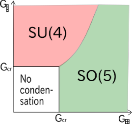
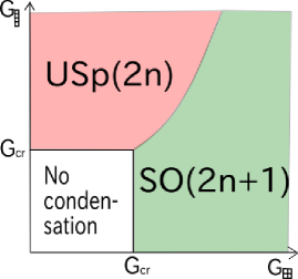
Figure 3: Odd $N=2n+1\geq 5$: $SU(2n+1)$ phase diagrams (rough sketch) are shown in the coupling constant $(G_{{\raisebox{-1.5pt}{\rule{3.0pt}{0.4pt}\hskip-3.0pt\rule{0.4pt}{3.0pt}\hskip 3.0pt\hskip-0.4pt\hskip-3.0pt\rule[3.0pt]{3.0pt}{0.4pt}\rule[3.0pt]{0.4pt}{0.4pt}\hskip-0.4pt\rule{0.4pt}{3.0pt}\hskip-0.4pt\rule{3.0pt}{0.4pt}\hskip-3.0pt\rule{0.4pt}{3.0pt}\hskip 3.0pt\hskip-0.4pt\hskip-3.0pt\rule[3.0pt]{3.0pt}{0.4pt}\rule[3.0pt]{0.4pt}{0.4pt}\hskip-0.4pt\rule{0.4pt}{3.0pt}\hskip-0.4pt}\hskip-6.0pt\raisebox{1.5pt}{\rule{3.0pt}{0.4pt}\hskip-3.0pt\rule{0.4pt}{3.0pt}\hskip 3.0pt\hskip-0.4pt\hskip-3.0pt\rule[3.0pt]{3.0pt}{0.4pt}\rule[3.0pt]{0.4pt}{0.4pt}\hskip-0.4pt\rule{0.4pt}{3.0pt}\hskip-0.4pt\rule{3.0pt}{0.4pt}\hskip-3.0pt\rule{0.4pt}{3.0pt}\hskip 3.0pt\hskip-0.4pt\hskip-3.0pt\rule[3.0pt]{3.0pt}{0.4pt}\rule[3.0pt]{0.4pt}{0.4pt}\hskip-0.4pt\rule{0.4pt}{3.0pt}\hskip-0.4pt}}},G_{{\raisebox{-3.0pt}{\raisebox{-1.5pt}{\rule{3.0pt}{0.4pt}\hskip-3.0pt\rule{0.4pt}{3.0pt}\hskip 3.0pt\hskip-0.4pt\hskip-3.0pt\rule[3.0pt]{3.0pt}{0.4pt}\rule[3.0pt]{0.4pt}{0.4pt}\hskip-0.4pt\rule{0.4pt}{3.0pt}\hskip-0.4pt}\hskip-3.0pt\raisebox{1.5pt}{\rule{3.0pt}{0.4pt}\hskip-3.0pt\rule{0.4pt}{3.0pt}\hskip 3.0pt\hskip-0.4pt\hskip-3.0pt\rule[3.0pt]{3.0pt}{0.4pt}\rule[3.0pt]{0.4pt}{0.4pt}\hskip-0.4pt\rule{0.4pt}{3.0pt}\hskip-0.4pt}}\hskip-3.0pt\raisebox{3.0pt}{\raisebox{-1.5pt}{\rule{3.0pt}{0.4pt}\hskip-3.0pt\rule{0.4pt}{3.0pt}\hskip 3.0pt\hskip-0.4pt\hskip-3.0pt\rule[3.0pt]{3.0pt}{0.4pt}\rule[3.0pt]{0.4pt}{0.4pt}\hskip-0.4pt\rule{0.4pt}{3.0pt}\hskip-0.4pt}\hskip-3.0pt\raisebox{1.5pt}{\rule{3.0pt}{0.4pt}\hskip-3.0pt\rule{0.4pt}{3.0pt}\hskip 3.0pt\hskip-0.4pt\hskip-3.0pt\rule[3.0pt]{3.0pt}{0.4pt}\rule[3.0pt]{0.4pt}{0.4pt}\hskip-0.4pt\rule{0.4pt}{3.0pt}\hskip-0.4pt}}}}\,)$ plane for $n=2$ (left figure) and $n\geq 3$ (right figure) cases.

Table 3: Branching rules of $SU(n)\supset SU(m=n-\ell)\times SU(\ell)\times U(1)$, $\ {}\supset SO(n)$, and $\ {}\supset USp(2n)$.

	$SU(n)$	$\supset$	$SU(n-\ell=m)\times SU(\ell)\times U(1)$
$\Big{|}$         :	n	=	$(\rule{7.0pt}{0.5pt}\hskip-7.0pt\rule{0.5pt}{7.0pt}\hskip 7.0pt\hskip-0.5pt\hskip-7.0pt\rule[7.0pt]{7.0pt}{0.5pt}\rule[7.0pt]{0.5pt}{0.5pt}\hskip-0.5pt\rule{0.5pt}{7.0pt}\hskip-0.5pt\,,\,{\bf 1})(\ell)\oplus({\bf 1},\,\rule{7.0pt}{0.5pt}\hskip-7.0pt\rule{0.5pt}{7.0pt}\hskip 7.0pt\hskip-0.5pt\hskip-7.0pt\rule[7.0pt]{7.0pt}{0.5pt}\rule[7.0pt]{0.5pt}{0.5pt}\hskip-0.5pt\rule{0.5pt}{7.0pt}\hskip-0.5pt)(-m)$
:	$\displaystyle\frac{\bf n(n+1)}{\bf 2}$	=	$\left(\rule{8.0pt}{0.5pt}\hskip-8.0pt\rule{0.5pt}{8.0pt}\hskip 8.0pt\hskip-0.5pt\hskip-8.0pt\rule[8.0pt]{8.0pt}{0.5pt}\rule[8.0pt]{0.5pt}{0.5pt}\hskip-0.5pt\rule{0.5pt}{8.0pt}\hskip-0.5pt\rule{8.0pt}{0.5pt}\hskip-8.0pt\rule{0.5pt}{8.0pt}\hskip 8.0pt\hskip-0.5pt\hskip-8.0pt\rule[8.0pt]{8.0pt}{0.5pt}\rule[8.0pt]{0.5pt}{0.5pt}\hskip-0.5pt\rule{0.5pt}{8.0pt}\hskip-0.5pt\,\,,\,{\bf 1}\right)(2\ell)\oplus\left(\rule{7.0pt}{0.5pt}\hskip-7.0pt\rule{0.5pt}{7.0pt}\hskip 7.0pt\hskip-0.5pt\hskip-7.0pt\rule[7.0pt]{7.0pt}{0.5pt}\rule[7.0pt]{0.5pt}{0.5pt}\hskip-0.5pt\rule{0.5pt}{7.0pt}\hskip-0.5pt\,,\,\rule{7.0pt}{0.5pt}\hskip-7.0pt\rule{0.5pt}{7.0pt}\hskip 7.0pt\hskip-0.5pt\hskip-7.0pt\rule[7.0pt]{7.0pt}{0.5pt}\rule[7.0pt]{0.5pt}{0.5pt}\hskip-0.5pt\rule{0.5pt}{7.0pt}\hskip-0.5pt\,\right)(\ell-m)\oplus\left({\bf 1},\,\rule{8.0pt}{0.5pt}\hskip-8.0pt\rule{0.5pt}{8.0pt}\hskip 8.0pt\hskip-0.5pt\hskip-8.0pt\rule[8.0pt]{8.0pt}{0.5pt}\rule[8.0pt]{0.5pt}{0.5pt}\hskip-0.5pt\rule{0.5pt}{8.0pt}\hskip-0.5pt\rule{8.0pt}{0.5pt}\hskip-8.0pt\rule{0.5pt}{8.0pt}\hskip 8.0pt\hskip-0.5pt\hskip-8.0pt\rule[8.0pt]{8.0pt}{0.5pt}\rule[8.0pt]{0.5pt}{0.5pt}\hskip-0.5pt\rule{0.5pt}{8.0pt}\hskip-0.5pt\,\,\right)(-2m)$
:	$\Bigg{|}$$\displaystyle\frac{{\bf n(n-1)}}{\bf 2}$	=	$\left(\rule{7.0pt}{0.5pt}\hskip-7.0pt\rule{0.5pt}{7.0pt}\hskip 7.0pt\hskip-0.5pt\hskip-7.0pt\rule[7.0pt]{7.0pt}{0.5pt}\rule[7.0pt]{0.5pt}{0.5pt}\hskip-0.5pt\rule{0.5pt}{7.0pt}\hskip-0.5pt\,,\,\rule{7.0pt}{0.5pt}\hskip-7.0pt\rule{0.5pt}{7.0pt}\hskip 7.0pt\hskip-0.5pt\hskip-7.0pt\rule[7.0pt]{7.0pt}{0.5pt}\rule[7.0pt]{0.5pt}{0.5pt}\hskip-0.5pt\rule{0.5pt}{7.0pt}\hskip-0.5pt\,\right)(\ell-m)\oplus\left(\raisebox{-3.5pt}{\rule{7.0pt}{0.5pt}\hskip-7.0pt\rule{0.5pt}{7.0pt}\hskip 7.0pt\hskip-0.5pt\hskip-7.0pt\rule[7.0pt]{7.0pt}{0.5pt}\rule[7.0pt]{0.5pt}{0.5pt}\hskip-0.5pt\rule{0.5pt}{7.0pt}\hskip-0.5pt}\hskip-7.0pt\raisebox{3.5pt}{\rule{7.0pt}{0.5pt}\hskip-7.0pt\rule{0.5pt}{7.0pt}\hskip 7.0pt\hskip-0.5pt\hskip-7.0pt\rule[7.0pt]{7.0pt}{0.5pt}\rule[7.0pt]{0.5pt}{0.5pt}\hskip-0.5pt\rule{0.5pt}{7.0pt}\hskip-0.5pt}\,,\,{\bf 1}\right)(2\ell)\oplus\left({\bf 1},\,\raisebox{-3.5pt}{\rule{7.0pt}{0.5pt}\hskip-7.0pt\rule{0.5pt}{7.0pt}\hskip 7.0pt\hskip-0.5pt\hskip-7.0pt\rule[7.0pt]{7.0pt}{0.5pt}\rule[7.0pt]{0.5pt}{0.5pt}\hskip-0.5pt\rule{0.5pt}{7.0pt}\hskip-0.5pt}\hskip-7.0pt\raisebox{3.5pt}{\rule{7.0pt}{0.5pt}\hskip-7.0pt\rule{0.5pt}{7.0pt}\hskip 7.0pt\hskip-0.5pt\hskip-7.0pt\rule[7.0pt]{7.0pt}{0.5pt}\rule[7.0pt]{0.5pt}{0.5pt}\hskip-0.5pt\rule{0.5pt}{7.0pt}\hskip-0.5pt}\,\right)(-2m)$
:	$\displaystyle\frac{\bf n^{2}(n+1)(n-1)}{\bf 12}$	=	$\left(\rule{8.0pt}{0.5pt}\hskip-8.0pt\rule{0.5pt}{8.0pt}\hskip 8.0pt\hskip-0.5pt\hskip-8.0pt\rule[8.0pt]{8.0pt}{0.5pt}\rule[8.0pt]{0.5pt}{0.5pt}\hskip-0.5pt\rule{0.5pt}{8.0pt}\hskip-0.5pt\rule{8.0pt}{0.5pt}\hskip-8.0pt\rule{0.5pt}{8.0pt}\hskip 8.0pt\hskip-0.5pt\hskip-8.0pt\rule[8.0pt]{8.0pt}{0.5pt}\rule[8.0pt]{0.5pt}{0.5pt}\hskip-0.5pt\rule{0.5pt}{8.0pt}\hskip-0.5pt\,\,,\,\rule{8.0pt}{0.5pt}\hskip-8.0pt\rule{0.5pt}{8.0pt}\hskip 8.0pt\hskip-0.5pt\hskip-8.0pt\rule[8.0pt]{8.0pt}{0.5pt}\rule[8.0pt]{0.5pt}{0.5pt}\hskip-0.5pt\rule{0.5pt}{8.0pt}\hskip-0.5pt\rule{8.0pt}{0.5pt}\hskip-8.0pt\rule{0.5pt}{8.0pt}\hskip 8.0pt\hskip-0.5pt\hskip-8.0pt\rule[8.0pt]{8.0pt}{0.5pt}\rule[8.0pt]{0.5pt}{0.5pt}\hskip-0.5pt\rule{0.5pt}{8.0pt}\hskip-0.5pt\,\,\right)(2\ell-2m)\oplus\left(\raisebox{-3.5pt}{\rule{7.0pt}{0.5pt}\hskip-7.0pt\rule{0.5pt}{7.0pt}\hskip 7.0pt\hskip-0.5pt\hskip-7.0pt\rule[7.0pt]{7.0pt}{0.5pt}\rule[7.0pt]{0.5pt}{0.5pt}\hskip-0.5pt\rule{0.5pt}{7.0pt}\hskip-0.5pt}\hskip-7.0pt\raisebox{3.5pt}{\rule{7.0pt}{0.5pt}\hskip-7.0pt\rule{0.5pt}{7.0pt}\hskip 7.0pt\hskip-0.5pt\hskip-7.0pt\rule[7.0pt]{7.0pt}{0.5pt}\rule[7.0pt]{0.5pt}{0.5pt}\hskip-0.5pt\rule{0.5pt}{7.0pt}\hskip-0.5pt\rule{7.0pt}{0.5pt}\hskip-7.0pt\rule{0.5pt}{7.0pt}\hskip 7.0pt\hskip-0.5pt\hskip-7.0pt\rule[7.0pt]{7.0pt}{0.5pt}\rule[7.0pt]{0.5pt}{0.5pt}\hskip-0.5pt\rule{0.5pt}{7.0pt}\hskip-0.5pt}\,\,,\,\rule{7.0pt}{0.5pt}\hskip-7.0pt\rule{0.5pt}{7.0pt}\hskip 7.0pt\hskip-0.5pt\hskip-7.0pt\rule[7.0pt]{7.0pt}{0.5pt}\rule[7.0pt]{0.5pt}{0.5pt}\hskip-0.5pt\rule{0.5pt}{7.0pt}\hskip-0.5pt\,\right)(3\ell-m)$
			$\oplus\left(\raisebox{-3.5pt}{\rule{7.0pt}{0.5pt}\hskip-7.0pt\rule{0.5pt}{7.0pt}\hskip 7.0pt\hskip-0.5pt\hskip-7.0pt\rule[7.0pt]{7.0pt}{0.5pt}\rule[7.0pt]{0.5pt}{0.5pt}\hskip-0.5pt\rule{0.5pt}{7.0pt}\hskip-0.5pt\rule{7.0pt}{0.5pt}\hskip-7.0pt\rule{0.5pt}{7.0pt}\hskip 7.0pt\hskip-0.5pt\hskip-7.0pt\rule[7.0pt]{7.0pt}{0.5pt}\rule[7.0pt]{0.5pt}{0.5pt}\hskip-0.5pt\rule{0.5pt}{7.0pt}\hskip-0.5pt}\hskip-14.0pt\raisebox{3.5pt}{\rule{7.0pt}{0.5pt}\hskip-7.0pt\rule{0.5pt}{7.0pt}\hskip 7.0pt\hskip-0.5pt\hskip-7.0pt\rule[7.0pt]{7.0pt}{0.5pt}\rule[7.0pt]{0.5pt}{0.5pt}\hskip-0.5pt\rule{0.5pt}{7.0pt}\hskip-0.5pt\rule{7.0pt}{0.5pt}\hskip-7.0pt\rule{0.5pt}{7.0pt}\hskip 7.0pt\hskip-0.5pt\hskip-7.0pt\rule[7.0pt]{7.0pt}{0.5pt}\rule[7.0pt]{0.5pt}{0.5pt}\hskip-0.5pt\rule{0.5pt}{7.0pt}\hskip-0.5pt}\,\,,\,{\bf 1}\right)(4\ell)\oplus\left(\rule{7.0pt}{0.5pt}\hskip-7.0pt\rule{0.5pt}{7.0pt}\hskip 7.0pt\hskip-0.5pt\hskip-7.0pt\rule[7.0pt]{7.0pt}{0.5pt}\rule[7.0pt]{0.5pt}{0.5pt}\hskip-0.5pt\rule{0.5pt}{7.0pt}\hskip-0.5pt\,,\,\raisebox{-3.5pt}{\rule{7.0pt}{0.5pt}\hskip-7.0pt\rule{0.5pt}{7.0pt}\hskip 7.0pt\hskip-0.5pt\hskip-7.0pt\rule[7.0pt]{7.0pt}{0.5pt}\rule[7.0pt]{0.5pt}{0.5pt}\hskip-0.5pt\rule{0.5pt}{7.0pt}\hskip-0.5pt}\hskip-7.0pt\raisebox{3.5pt}{\rule{7.0pt}{0.5pt}\hskip-7.0pt\rule{0.5pt}{7.0pt}\hskip 7.0pt\hskip-0.5pt\hskip-7.0pt\rule[7.0pt]{7.0pt}{0.5pt}\rule[7.0pt]{0.5pt}{0.5pt}\hskip-0.5pt\rule{0.5pt}{7.0pt}\hskip-0.5pt\rule{7.0pt}{0.5pt}\hskip-7.0pt\rule{0.5pt}{7.0pt}\hskip 7.0pt\hskip-0.5pt\hskip-7.0pt\rule[7.0pt]{7.0pt}{0.5pt}\rule[7.0pt]{0.5pt}{0.5pt}\hskip-0.5pt\rule{0.5pt}{7.0pt}\hskip-0.5pt}\,\,\right)(\ell-3m)$
			$\oplus\left(\raisebox{-3.5pt}{\rule{7.0pt}{0.5pt}\hskip-7.0pt\rule{0.5pt}{7.0pt}\hskip 7.0pt\hskip-0.5pt\hskip-7.0pt\rule[7.0pt]{7.0pt}{0.5pt}\rule[7.0pt]{0.5pt}{0.5pt}\hskip-0.5pt\rule{0.5pt}{7.0pt}\hskip-0.5pt}\hskip-7.0pt\raisebox{3.5pt}{\rule{7.0pt}{0.5pt}\hskip-7.0pt\rule{0.5pt}{7.0pt}\hskip 7.0pt\hskip-0.5pt\hskip-7.0pt\rule[7.0pt]{7.0pt}{0.5pt}\rule[7.0pt]{0.5pt}{0.5pt}\hskip-0.5pt\rule{0.5pt}{7.0pt}\hskip-0.5pt}\,,\,\raisebox{-3.5pt}{\rule{7.0pt}{0.5pt}\hskip-7.0pt\rule{0.5pt}{7.0pt}\hskip 7.0pt\hskip-0.5pt\hskip-7.0pt\rule[7.0pt]{7.0pt}{0.5pt}\rule[7.0pt]{0.5pt}{0.5pt}\hskip-0.5pt\rule{0.5pt}{7.0pt}\hskip-0.5pt}\hskip-7.0pt\raisebox{3.5pt}{\rule{7.0pt}{0.5pt}\hskip-7.0pt\rule{0.5pt}{7.0pt}\hskip 7.0pt\hskip-0.5pt\hskip-7.0pt\rule[7.0pt]{7.0pt}{0.5pt}\rule[7.0pt]{0.5pt}{0.5pt}\hskip-0.5pt\rule{0.5pt}{7.0pt}\hskip-0.5pt}\,\right)(2\ell-2m)\oplus\left({\bf 1},\,\raisebox{-3.5pt}{\rule{7.0pt}{0.5pt}\hskip-7.0pt\rule{0.5pt}{7.0pt}\hskip 7.0pt\hskip-0.5pt\hskip-7.0pt\rule[7.0pt]{7.0pt}{0.5pt}\rule[7.0pt]{0.5pt}{0.5pt}\hskip-0.5pt\rule{0.5pt}{7.0pt}\hskip-0.5pt\rule{7.0pt}{0.5pt}\hskip-7.0pt\rule{0.5pt}{7.0pt}\hskip 7.0pt\hskip-0.5pt\hskip-7.0pt\rule[7.0pt]{7.0pt}{0.5pt}\rule[7.0pt]{0.5pt}{0.5pt}\hskip-0.5pt\rule{0.5pt}{7.0pt}\hskip-0.5pt}\hskip-14.0pt\raisebox{3.5pt}{\rule{7.0pt}{0.5pt}\hskip-7.0pt\rule{0.5pt}{7.0pt}\hskip 7.0pt\hskip-0.5pt\hskip-7.0pt\rule[7.0pt]{7.0pt}{0.5pt}\rule[7.0pt]{0.5pt}{0.5pt}\hskip-0.5pt\rule{0.5pt}{7.0pt}\hskip-0.5pt\rule{7.0pt}{0.5pt}\hskip-7.0pt\rule{0.5pt}{7.0pt}\hskip 7.0pt\hskip-0.5pt\hskip-7.0pt\rule[7.0pt]{7.0pt}{0.5pt}\rule[7.0pt]{0.5pt}{0.5pt}\hskip-0.5pt\rule{0.5pt}{7.0pt}\hskip-0.5pt}\,\,\right)(-4m)$
:	$\displaystyle\frac{\bf n(n-1)(n-2)(n-3)}{\bf 24}$	=	$\left(\rule{7.0pt}{0.5pt}\hskip-7.0pt\rule{0.5pt}{7.0pt}\hskip 7.0pt\hskip-0.5pt\hskip-7.0pt\rule[7.0pt]{7.0pt}{0.5pt}\rule[7.0pt]{0.5pt}{0.5pt}\hskip-0.5pt\rule{0.5pt}{7.0pt}\hskip-0.5pt\,,\,\raisebox{-7.0pt}{\rule{7.0pt}{0.5pt}\hskip-7.0pt\rule{0.5pt}{7.0pt}\hskip 7.0pt\hskip-0.5pt\hskip-7.0pt\rule[7.0pt]{7.0pt}{0.5pt}\rule[7.0pt]{0.5pt}{0.5pt}\hskip-0.5pt\rule{0.5pt}{7.0pt}\hskip-0.5pt}\hskip-7.0pt\raisebox{3.5pt}{\raisebox{-3.5pt}{\rule{7.0pt}{0.5pt}\hskip-7.0pt\rule{0.5pt}{7.0pt}\hskip 7.0pt\hskip-0.5pt\hskip-7.0pt\rule[7.0pt]{7.0pt}{0.5pt}\rule[7.0pt]{0.5pt}{0.5pt}\hskip-0.5pt\rule{0.5pt}{7.0pt}\hskip-0.5pt}\hskip-7.0pt\raisebox{3.5pt}{\rule{7.0pt}{0.5pt}\hskip-7.0pt\rule{0.5pt}{7.0pt}\hskip 7.0pt\hskip-0.5pt\hskip-7.0pt\rule[7.0pt]{7.0pt}{0.5pt}\rule[7.0pt]{0.5pt}{0.5pt}\hskip-0.5pt\rule{0.5pt}{7.0pt}\hskip-0.5pt}}\,\right)(\ell-3m)\oplus\left(\raisebox{-3.5pt}{\rule{7.0pt}{0.5pt}\hskip-7.0pt\rule{0.5pt}{7.0pt}\hskip 7.0pt\hskip-0.5pt\hskip-7.0pt\rule[7.0pt]{7.0pt}{0.5pt}\rule[7.0pt]{0.5pt}{0.5pt}\hskip-0.5pt\rule{0.5pt}{7.0pt}\hskip-0.5pt}\hskip-7.0pt\raisebox{3.5pt}{\rule{7.0pt}{0.5pt}\hskip-7.0pt\rule{0.5pt}{7.0pt}\hskip 7.0pt\hskip-0.5pt\hskip-7.0pt\rule[7.0pt]{7.0pt}{0.5pt}\rule[7.0pt]{0.5pt}{0.5pt}\hskip-0.5pt\rule{0.5pt}{7.0pt}\hskip-0.5pt}\,,\,\raisebox{-3.5pt}{\rule{7.0pt}{0.5pt}\hskip-7.0pt\rule{0.5pt}{7.0pt}\hskip 7.0pt\hskip-0.5pt\hskip-7.0pt\rule[7.0pt]{7.0pt}{0.5pt}\rule[7.0pt]{0.5pt}{0.5pt}\hskip-0.5pt\rule{0.5pt}{7.0pt}\hskip-0.5pt}\hskip-7.0pt\raisebox{3.5pt}{\rule{7.0pt}{0.5pt}\hskip-7.0pt\rule{0.5pt}{7.0pt}\hskip 7.0pt\hskip-0.5pt\hskip-7.0pt\rule[7.0pt]{7.0pt}{0.5pt}\rule[7.0pt]{0.5pt}{0.5pt}\hskip-0.5pt\rule{0.5pt}{7.0pt}\hskip-0.5pt}\,\right)(2\ell-2m)$
			$\oplus\left(\raisebox{-7.0pt}{\rule{7.0pt}{0.5pt}\hskip-7.0pt\rule{0.5pt}{7.0pt}\hskip 7.0pt\hskip-0.5pt\hskip-7.0pt\rule[7.0pt]{7.0pt}{0.5pt}\rule[7.0pt]{0.5pt}{0.5pt}\hskip-0.5pt\rule{0.5pt}{7.0pt}\hskip-0.5pt}\hskip-7.0pt\raisebox{3.5pt}{\raisebox{-3.5pt}{\rule{7.0pt}{0.5pt}\hskip-7.0pt\rule{0.5pt}{7.0pt}\hskip 7.0pt\hskip-0.5pt\hskip-7.0pt\rule[7.0pt]{7.0pt}{0.5pt}\rule[7.0pt]{0.5pt}{0.5pt}\hskip-0.5pt\rule{0.5pt}{7.0pt}\hskip-0.5pt}\hskip-7.0pt\raisebox{3.5pt}{\rule{7.0pt}{0.5pt}\hskip-7.0pt\rule{0.5pt}{7.0pt}\hskip 7.0pt\hskip-0.5pt\hskip-7.0pt\rule[7.0pt]{7.0pt}{0.5pt}\rule[7.0pt]{0.5pt}{0.5pt}\hskip-0.5pt\rule{0.5pt}{7.0pt}\hskip-0.5pt}}\,,\,\rule{7.0pt}{0.5pt}\hskip-7.0pt\rule{0.5pt}{7.0pt}\hskip 7.0pt\hskip-0.5pt\hskip-7.0pt\rule[7.0pt]{7.0pt}{0.5pt}\rule[7.0pt]{0.5pt}{0.5pt}\hskip-0.5pt\rule{0.5pt}{7.0pt}\hskip-0.5pt\,\right)(3\ell-m)\oplus\left(\raisebox{-7.0pt}{\raisebox{-3.5pt}{\rule{7.0pt}{0.5pt}\hskip-7.0pt\rule{0.5pt}{7.0pt}\hskip 7.0pt\hskip-0.5pt\hskip-7.0pt\rule[7.0pt]{7.0pt}{0.5pt}\rule[7.0pt]{0.5pt}{0.5pt}\hskip-0.5pt\rule{0.5pt}{7.0pt}\hskip-0.5pt}\hskip-7.0pt\raisebox{3.5pt}{\rule{7.0pt}{0.5pt}\hskip-7.0pt\rule{0.5pt}{7.0pt}\hskip 7.0pt\hskip-0.5pt\hskip-7.0pt\rule[7.0pt]{7.0pt}{0.5pt}\rule[7.0pt]{0.5pt}{0.5pt}\hskip-0.5pt\rule{0.5pt}{7.0pt}\hskip-0.5pt}}\hskip-7.0pt\raisebox{7.0pt}{\raisebox{-3.5pt}{\rule{7.0pt}{0.5pt}\hskip-7.0pt\rule{0.5pt}{7.0pt}\hskip 7.0pt\hskip-0.5pt\hskip-7.0pt\rule[7.0pt]{7.0pt}{0.5pt}\rule[7.0pt]{0.5pt}{0.5pt}\hskip-0.5pt\rule{0.5pt}{7.0pt}\hskip-0.5pt}\hskip-7.0pt\raisebox{3.5pt}{\rule{7.0pt}{0.5pt}\hskip-7.0pt\rule{0.5pt}{7.0pt}\hskip 7.0pt\hskip-0.5pt\hskip-7.0pt\rule[7.0pt]{7.0pt}{0.5pt}\rule[7.0pt]{0.5pt}{0.5pt}\hskip-0.5pt\rule{0.5pt}{7.0pt}\hskip-0.5pt}}\,\,,\,{\bf 1}\right)(4\ell)\oplus\left({\bf 1},\,\raisebox{-7.0pt}{\raisebox{-3.5pt}{\rule{7.0pt}{0.5pt}\hskip-7.0pt\rule{0.5pt}{7.0pt}\hskip 7.0pt\hskip-0.5pt\hskip-7.0pt\rule[7.0pt]{7.0pt}{0.5pt}\rule[7.0pt]{0.5pt}{0.5pt}\hskip-0.5pt\rule{0.5pt}{7.0pt}\hskip-0.5pt}\hskip-7.0pt\raisebox{3.5pt}{\rule{7.0pt}{0.5pt}\hskip-7.0pt\rule{0.5pt}{7.0pt}\hskip 7.0pt\hskip-0.5pt\hskip-7.0pt\rule[7.0pt]{7.0pt}{0.5pt}\rule[7.0pt]{0.5pt}{0.5pt}\hskip-0.5pt\rule{0.5pt}{7.0pt}\hskip-0.5pt}}\hskip-7.0pt\raisebox{7.0pt}{\raisebox{-3.5pt}{\rule{7.0pt}{0.5pt}\hskip-7.0pt\rule{0.5pt}{7.0pt}\hskip 7.0pt\hskip-0.5pt\hskip-7.0pt\rule[7.0pt]{7.0pt}{0.5pt}\rule[7.0pt]{0.5pt}{0.5pt}\hskip-0.5pt\rule{0.5pt}{7.0pt}\hskip-0.5pt}\hskip-7.0pt\raisebox{3.5pt}{\rule{7.0pt}{0.5pt}\hskip-7.0pt\rule{0.5pt}{7.0pt}\hskip 7.0pt\hskip-0.5pt\hskip-7.0pt\rule[7.0pt]{7.0pt}{0.5pt}\rule[7.0pt]{0.5pt}{0.5pt}\hskip-0.5pt\rule{0.5pt}{7.0pt}\hskip-0.5pt}}\,\,\right)(-4m)$
	$\dim\raisebox{-3.5pt}{\rule{7.0pt}{0.5pt}\hskip-7.0pt\rule{0.5pt}{7.0pt}\hskip 7.0pt\hskip-0.5pt\hskip-7.0pt\rule[7.0pt]{7.0pt}{0.5pt}\rule[7.0pt]{0.5pt}{0.5pt}\hskip-0.5pt\rule{0.5pt}{7.0pt}\hskip-0.5pt}\hskip-7.0pt\raisebox{3.5pt}{\rule{7.0pt}{0.5pt}\hskip-7.0pt\rule{0.5pt}{7.0pt}\hskip 7.0pt\hskip-0.5pt\hskip-7.0pt\rule[7.0pt]{7.0pt}{0.5pt}\rule[7.0pt]{0.5pt}{0.5pt}\hskip-0.5pt\rule{0.5pt}{7.0pt}\hskip-0.5pt\rule{7.0pt}{0.5pt}\hskip-7.0pt\rule{0.5pt}{7.0pt}\hskip 7.0pt\hskip-0.5pt\hskip-7.0pt\rule[7.0pt]{7.0pt}{0.5pt}\rule[7.0pt]{0.5pt}{0.5pt}\hskip-0.5pt\rule{0.5pt}{7.0pt}\hskip-0.5pt}\,={\rule[-5.37498pt]{0.0pt}{19.88887pt}\hbox{$\displaystyle\frac{\bf n(n^{2}-1)}{\bf 3}$}}$		$\dim\raisebox{-7.0pt}{\rule{7.0pt}{0.5pt}\hskip-7.0pt\rule{0.5pt}{7.0pt}\hskip 7.0pt\hskip-0.5pt\hskip-7.0pt\rule[7.0pt]{7.0pt}{0.5pt}\rule[7.0pt]{0.5pt}{0.5pt}\hskip-0.5pt\rule{0.5pt}{7.0pt}\hskip-0.5pt}\hskip-7.0pt\raisebox{3.5pt}{\raisebox{-3.5pt}{\rule{7.0pt}{0.5pt}\hskip-7.0pt\rule{0.5pt}{7.0pt}\hskip 7.0pt\hskip-0.5pt\hskip-7.0pt\rule[7.0pt]{7.0pt}{0.5pt}\rule[7.0pt]{0.5pt}{0.5pt}\hskip-0.5pt\rule{0.5pt}{7.0pt}\hskip-0.5pt}\hskip-7.0pt\raisebox{3.5pt}{\rule{7.0pt}{0.5pt}\hskip-7.0pt\rule{0.5pt}{7.0pt}\hskip 7.0pt\hskip-0.5pt\hskip-7.0pt\rule[7.0pt]{7.0pt}{0.5pt}\rule[7.0pt]{0.5pt}{0.5pt}\hskip-0.5pt\rule{0.5pt}{7.0pt}\hskip-0.5pt}}=\displaystyle\frac{\bf n(n-1)(n-2)}{\bf 6}$  for $SU(n)$
	$SU(n)$	$\supset$	$SO(n)$
:	n	=	n
:	${\bf\displaystyle\frac{n(n+1)}{2}}$	=	${\bf\displaystyle\frac{(n-1)(n+2)}{2}}\oplus{\bf 1}$
:	$\Bigg{|}$ ${\bf\displaystyle\frac{n(n-1)}{2}}$	=	${\bf\displaystyle\frac{n(n-1)}{2}}$
:	${\bf\displaystyle\frac{n^{2}(n+1)(n-1)}{12}}$	=	${\bf\displaystyle\frac{n(n+1)(n+2)(n-3)}{12}}\oplus{\bf\displaystyle\frac{{(n-1)}(n+2)}{2}}\oplus{\bf 1}$
:	${\bf\displaystyle\frac{n(n-1)(n-2)(n-3)}{24}}$	=	${\bf\displaystyle\frac{n(n-1)(n-2)(n-3)}{24}}$.
	$SU(2n)$	$\supset$	$USp(2n)$
:	2n	=	2n
:	${\bf n(2n+1)}$	=	${\bf n(2n+1)}$
:	$\bigg{|}$${\bf n(2n-1)}$	=	${\bf(n-1)(2n+1)}\oplus{\bf 1}$
:	${\bf\displaystyle\frac{n^{2}(2n+1)(2n-1)}{3}}$	=	${\bf\displaystyle\frac{n(n-1)(2n-1)(2n+3)}{3}}\oplus{\bf(n-1)(2n+1)}\oplus{\bf 1}$
:	${\bf\displaystyle\frac{n(n-1)(2n-1)(2n-3)}{6}}$	=	${\bf\displaystyle\frac{n(n-3)(2n+1)(2n-1)}{6}}\oplus{\bf(n-1)(2n+1)}\oplus{\bf 1}$

Table 4: Branching rules of $SU(8)\supset SU(4)\times SU(2)$ and $SU(16)\supset SO(10)$.

	$SU(8)$	$\supset$	$SU(4)\times SU(2)$
:	8	=	$({\bf 4,2})$
:	${\bf 36}$	=	$({\bf 10,3})\oplus({\bf 6,1})$
:	${\bf 28}$	=	$({\bf 10,1})\oplus({\bf 6,3})$
:	${\bf 336}$	=	$({\bf 35,1})\oplus({\bf 45,3})\oplus({\bf 20^{\prime},5})\oplus({\bf 20^{\prime},1})\oplus({\bf 15,3})\oplus({\bf 1,1})$
:	${\bf 70}$	=	$({\bf 20^{\prime},1})\oplus({\bf 15,3})\oplus({\bf 1,5})$
	$SU(16)$	$\supset$	$SO(10)$
:	${\bf 16}$	=	$({\bf 16})$
:	${\bf 136}$	=	$({\bf\overline{126}})\oplus({\bf 10})$
:	${\bf 120}$	=	$({\bf 120})$
:	${\bf 5440}$	=	$({\bf 4125})\oplus({\bf\overline{1050}})\oplus({\bf 54})\oplus({\bf 210})\oplus({\bf 1})$
:	${\bf 1820}$	=	$({\bf 770})\oplus({\bf 1050})$

5 Summary and discussions

We have performed the potential analysis of the $SU(N)$ NJL type models for two cases with a fermion in an $SU(N)$ defining representation ${\boldsymbol{R}}=\rule{8.0pt}{0.5pt}\hskip-8.0pt\rule{0.5pt}{8.0pt}\hskip 8.0pt\hskip-0.5pt\hskip-8.0pt\rule[8.0pt]{8.0pt}{0.5pt}\rule[8.0pt]{0.5pt}{0.5pt}\hskip-0.5pt\rule{0.5pt}{8.0pt}\hskip-0.5pt\,$ and an $SU(N)$ rank-2 anti-symmetric representation ${\boldsymbol{R}}={\raisebox{-3.5pt}{\rule{7.0pt}{0.5pt}\hskip-7.0pt\rule{0.5pt}{7.0pt}\hskip 7.0pt\hskip-0.5pt\hskip-7.0pt\rule[7.0pt]{7.0pt}{0.5pt}\rule[7.0pt]{0.5pt}{0.5pt}\hskip-0.5pt\rule{0.5pt}{7.0pt}\hskip-0.5pt}\hskip-7.0pt\raisebox{3.5pt}{\rule{7.0pt}{0.5pt}\hskip-7.0pt\rule{0.5pt}{7.0pt}\hskip 7.0pt\hskip-0.5pt\hskip-7.0pt\rule[7.0pt]{7.0pt}{0.5pt}\rule[7.0pt]{0.5pt}{0.5pt}\hskip-0.5pt\rule{0.5pt}{7.0pt}\hskip-0.5pt}}\,\$, respectively.

The former case with ${\boldsymbol{R}}=\rule{8.0pt}{0.5pt}\hskip-8.0pt\rule{0.5pt}{8.0pt}\hskip 8.0pt\hskip-0.5pt\hskip-8.0pt\rule[8.0pt]{8.0pt}{0.5pt}\rule[8.0pt]{0.5pt}{0.5pt}\hskip-0.5pt\rule{0.5pt}{8.0pt}\hskip-0.5pt\,$ fermion shows that at the potential minimum the $SU(N)$ group symmetry is always broken to its special subgroup $SO(N)$ as far as the symmetry breaking occurs. The latter case with ${\boldsymbol{R}}={\raisebox{-3.5pt}{\rule{7.0pt}{0.5pt}\hskip-7.0pt\rule{0.5pt}{7.0pt}\hskip 7.0pt\hskip-0.5pt\hskip-7.0pt\rule[7.0pt]{7.0pt}{0.5pt}\rule[7.0pt]{0.5pt}{0.5pt}\hskip-0.5pt\rule{0.5pt}{7.0pt}\hskip-0.5pt}\hskip-7.0pt\raisebox{3.5pt}{\rule{7.0pt}{0.5pt}\hskip-7.0pt\rule{0.5pt}{7.0pt}\hskip 7.0pt\hskip-0.5pt\hskip-7.0pt\rule[7.0pt]{7.0pt}{0.5pt}\rule[7.0pt]{0.5pt}{0.5pt}\hskip-0.5pt\rule{0.5pt}{7.0pt}\hskip-0.5pt}}\,\$ also shows that the $SU(N)$ symmetry for $N\geq 4$ is, if broken, always broken to its special subgroup $SO(N)$ or $USp(2[N/2])$ aside from some exceptional cases; for $N=4$ the $SU(4)$ symmetry is broken to its special subgroup $SO(4)$ or is not broken although the condensation into $SU(4)$-singlet occurs; for $N=16$ the $SU(16)$ is broken to its special subgroup $SO(16)$ or $SO(10)$ or $USp(16)$; for $N=5$ the $SU(5)$ is broken to its special subgroup $SO(5)$ or to a regular subgroup $SU(4)$; for $N=3$ the $SU(3)$ is broken to its special subgroup $SO(3)$. That is, aside from the only breaking $SU(5)\rightarrow SU(4)$ for $N=5$, all the $SU(N)$ symmetry breakings for $N\geq 3$ is down to its special subgroups in the case ${\boldsymbol{R}}={\raisebox{-3.5pt}{\rule{7.0pt}{0.5pt}\hskip-7.0pt\rule{0.5pt}{7.0pt}\hskip 7.0pt\hskip-0.5pt\hskip-7.0pt\rule[7.0pt]{7.0pt}{0.5pt}\rule[7.0pt]{0.5pt}{0.5pt}\hskip-0.5pt\rule{0.5pt}{7.0pt}\hskip-0.5pt}\hskip-7.0pt\raisebox{3.5pt}{\rule{7.0pt}{0.5pt}\hskip-7.0pt\rule{0.5pt}{7.0pt}\hskip 7.0pt\hskip-0.5pt\hskip-7.0pt\rule[7.0pt]{7.0pt}{0.5pt}\rule[7.0pt]{0.5pt}{0.5pt}\hskip-0.5pt\rule{0.5pt}{7.0pt}\hskip-0.5pt}}\,\$.

This result clearly shows that symmetry breaking into special subgroups is not special at all at least for the dynamical symmetry breaking in the 4D NJL type model. One might, however, suspect that this may be a special situation specific to the classical group $G=SU(N)$ model. But, actually, this tendency of symmetry breaking to special subgroups was found previously for the exceptional group $G=E_{6}$ model in Ref. [58]. They analyzed the potential in the 4D $E_{6}$ NJL model with fundamental representation ${\boldsymbol{R}}={\bf 27}$ fermion, which have two coupling constants $G_{\bf 27}$ and $G_{\bf 351^{\prime}}$ since $({\bf 27}\times{\bf 27})_{S}=\overline{\bf 27}+\overline{\bf 351^{\prime}}$. The result of their potential analysis is summarized in the $E_{6}$ phase diagram shown in Figure 4.

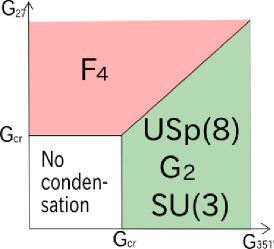
Figure 4: $E_{6}$ phase diagrams are shown in the coupling constant $(G_{351^{\prime}},\,G_{27})$ plane.

This result is very similar to the breaking pattern in our $SU(16)$ case with                  fermion shown in Figure 2.

First of all, all the groups $F_{4}$, $USp(8)$, $G_{2}$ and $SU(3)$ appearing here in Figure 4 are special subgroups, and the breaking into the regular subgroup $SO(10)=E_{5}$ does not occur at all despite that $SO(10)$ is one of the maximal little groups of scalar $\Phi_{\bf 27}$ or $\Phi_{\bf 351^{\prime}}$. Moreover, the 27 fermion falls into a single irreducible representation 27 under the special subgroups $USp(8)$, $G_{2}$ and $SU(3)$ while it splits into two ${\bf 26}+{\bf 1}$ under $F_{4}$. This is very much parallel to the situation in our $SU(16)$ case that the                  fermion 120 falls into a single representation 120 also under the $SO(16)$ and $SO(10)$ subgroups, while it splits into ${\bf 119}+{\bf 1}$ under $USp(16)$. In particular, the fact that the irreducible representation fermion of $G$ also falls into a single irreducible representation under distinct plural subgroups $H$ implies in this NJL model the special existence of degenerate broken vacua; $USp(8)$, $G_{2}$ and $SU(3)$ vacua for the $G=E_{6}$ case, and $SO(16)$ and $SO(10)$ vacua for $G=SU(16)$ case. For the $E_{6}$ case, however, numerical study showed the surprising fact that the general vacuum does not show any of the symmetries $USp(8)$, or $G_{2}$ or $SU(3)$. The authors of Ref. [58] conjectured the existence of the continuous path in the scalar $\Phi_{\bf 351^{\prime}}$ space connecting those three vacua of $USp(8)$, $G_{2}$ and $SU(3)$ through which the potential is flat and the $E_{6}$ symmetry is totally broken in between those three points. Although this was a conjecture for the $E_{6}$ case, we can show explicitly that it is really the case for our $SU(16)\rightarrow SO(16),SO(10)$ breaking case. We have shown this analytically in Appendix by constructing the one-parameter vacua which connect the $SO(16)$ and $SO(10)$ vacua and realize the degenerate lowest potential energy. Explicit computation of the $SU(16)$ gauge boson mass square matrix was given for the $SO(16)$ and $SO(10)$ vacua which suggests the total breaking of $SU(16)$ symmetry for the general parameter vacua between the $SO(16)$ and $SO(10)$ vacua.

Appendix A Degeneracy between SO(16) and SO(10) vacua in the SU(16) NJL model

As stated in the text, the NJL model with rank-2 anti-symmetric fermion $\psi_{\raisebox{-1.5pt}{\rule{3.0pt}{0.4pt}\hskip-3.0pt\rule{0.4pt}{3.0pt}\hskip 3.0pt\hskip-0.4pt\hskip-3.0pt\rule[3.0pt]{3.0pt}{0.4pt}\rule[3.0pt]{0.4pt}{0.4pt}\hskip-0.4pt\rule{0.4pt}{3.0pt}\hskip-0.4pt}\hskip-3.0pt\raisebox{1.5pt}{\rule{3.0pt}{0.4pt}\hskip-3.0pt\rule{0.4pt}{3.0pt}\hskip 3.0pt\hskip-0.4pt\hskip-3.0pt\rule[3.0pt]{3.0pt}{0.4pt}\rule[3.0pt]{0.4pt}{0.4pt}\hskip-0.4pt\rule{0.4pt}{3.0pt}\hskip-0.4pt}}=\psi_{I}=\psi_{ij}$ for $G=SU(N{=}16)$, is broken into the $SO(N{=}16)$-invariant vacuum, when $G_{\raisebox{-1.5pt}{\rule{3.0pt}{0.4pt}\hskip-3.0pt\rule{0.4pt}{3.0pt}\hskip 3.0pt\hskip-0.4pt\hskip-3.0pt\rule[3.0pt]{3.0pt}{0.4pt}\rule[3.0pt]{0.4pt}{0.4pt}\hskip-0.4pt\rule{0.4pt}{3.0pt}\hskip-0.4pt\rule{3.0pt}{0.4pt}\hskip-3.0pt\rule{0.4pt}{3.0pt}\hskip 3.0pt\hskip-0.4pt\hskip-3.0pt\rule[3.0pt]{3.0pt}{0.4pt}\rule[3.0pt]{0.4pt}{0.4pt}\hskip-0.4pt\rule{0.4pt}{3.0pt}\hskip-0.4pt}\hskip-6.0pt\raisebox{1.5pt}{\rule{3.0pt}{0.4pt}\hskip-3.0pt\rule{0.4pt}{3.0pt}\hskip 3.0pt\hskip-0.4pt\hskip-3.0pt\rule[3.0pt]{3.0pt}{0.4pt}\rule[3.0pt]{0.4pt}{0.4pt}\hskip-0.4pt\rule{0.4pt}{3.0pt}\hskip-0.4pt\rule{3.0pt}{0.4pt}\hskip-3.0pt\rule{0.4pt}{3.0pt}\hskip 3.0pt\hskip-0.4pt\hskip-3.0pt\rule[3.0pt]{3.0pt}{0.4pt}\rule[3.0pt]{0.4pt}{0.4pt}\hskip-0.4pt\rule{0.4pt}{3.0pt}\hskip-0.4pt}}>G_{\raisebox{-3.0pt}{\raisebox{-1.5pt}{\rule{3.0pt}{0.4pt}\hskip-3.0pt\rule{0.4pt}{3.0pt}\hskip 3.0pt\hskip-0.4pt\hskip-3.0pt\rule[3.0pt]{3.0pt}{0.4pt}\rule[3.0pt]{0.4pt}{0.4pt}\hskip-0.4pt\rule{0.4pt}{3.0pt}\hskip-0.4pt}\hskip-3.0pt\raisebox{1.5pt}{\rule{3.0pt}{0.4pt}\hskip-3.0pt\rule{0.4pt}{3.0pt}\hskip 3.0pt\hskip-0.4pt\hskip-3.0pt\rule[3.0pt]{3.0pt}{0.4pt}\rule[3.0pt]{0.4pt}{0.4pt}\hskip-0.4pt\rule{0.4pt}{3.0pt}\hskip-0.4pt}}\hskip-3.0pt\raisebox{3.0pt}{\raisebox{-1.5pt}{\rule{3.0pt}{0.4pt}\hskip-3.0pt\rule{0.4pt}{3.0pt}\hskip 3.0pt\hskip-0.4pt\hskip-3.0pt\rule[3.0pt]{3.0pt}{0.4pt}\rule[3.0pt]{0.4pt}{0.4pt}\hskip-0.4pt\rule{0.4pt}{3.0pt}\hskip-0.4pt}\hskip-3.0pt\raisebox{1.5pt}{\rule{3.0pt}{0.4pt}\hskip-3.0pt\rule{0.4pt}{3.0pt}\hskip 3.0pt\hskip-0.4pt\hskip-3.0pt\rule[3.0pt]{3.0pt}{0.4pt}\rule[3.0pt]{0.4pt}{0.4pt}\hskip-0.4pt\rule{0.4pt}{3.0pt}\hskip-0.4pt}}}$ as usual for any $N$, realizing the VEV

$$\left\langle{{\Phi_{\raisebox{-1.5pt}{\rule{3.0pt}{0.4pt}\hskip-3.0pt\rule{0.4pt}{3.0pt}\hskip 3.0pt\hskip-0.4pt\hskip-3.0pt\rule[3.0pt]{3.0pt}{0.4pt}\rule[3.0pt]{0.4pt}{0.4pt}\hskip-0.4pt\rule{0.4pt}{3.0pt}\hskip-0.4pt\rule{3.0pt}{0.4pt}\hskip-3.0pt\rule{0.4pt}{3.0pt}\hskip 3.0pt\hskip-0.4pt\hskip-3.0pt\rule[3.0pt]{3.0pt}{0.4pt}\rule[3.0pt]{0.4pt}{0.4pt}\hskip-0.4pt\rule{0.4pt}{3.0pt}\hskip-0.4pt}\hskip-6.0pt\raisebox{1.5pt}{\rule{3.0pt}{0.4pt}\hskip-3.0pt\rule{0.4pt}{3.0pt}\hskip 3.0pt\hskip-0.4pt\hskip-3.0pt\rule[3.0pt]{3.0pt}{0.4pt}\rule[3.0pt]{0.4pt}{0.4pt}\hskip-0.4pt\rule{0.4pt}{3.0pt}\hskip-0.4pt\rule{3.0pt}{0.4pt}\hskip-3.0pt\rule{0.4pt}{3.0pt}\hskip 3.0pt\hskip-0.4pt\hskip-3.0pt\rule[3.0pt]{3.0pt}{0.4pt}\rule[3.0pt]{0.4pt}{0.4pt}\hskip-0.4pt\rule{0.4pt}{3.0pt}\hskip-0.4pt}}\,}_{ij,kl}}\right\rangle^{\rm SO(N{=}16)}=\frac{v}{2}\delta_{ij}^{kl}=v\delta_{[i}^{k}\delta_{j]}^{l}\ .$$ (A.1)

For this $N=16$ case, however, $G=SU(16)$ can also be broken to the SO(10) vacuum possessing the VEV

$$\left\langle{{\Phi_{\raisebox{-1.5pt}{\rule{3.0pt}{0.4pt}\hskip-3.0pt\rule{0.4pt}{3.0pt}\hskip 3.0pt\hskip-0.4pt\hskip-3.0pt\rule[3.0pt]{3.0pt}{0.4pt}\rule[3.0pt]{0.4pt}{0.4pt}\hskip-0.4pt\rule{0.4pt}{3.0pt}\hskip-0.4pt\rule{3.0pt}{0.4pt}\hskip-3.0pt\rule{0.4pt}{3.0pt}\hskip 3.0pt\hskip-0.4pt\hskip-3.0pt\rule[3.0pt]{3.0pt}{0.4pt}\rule[3.0pt]{0.4pt}{0.4pt}\hskip-0.4pt\rule{0.4pt}{3.0pt}\hskip-0.4pt}\hskip-6.0pt\raisebox{1.5pt}{\rule{3.0pt}{0.4pt}\hskip-3.0pt\rule{0.4pt}{3.0pt}\hskip 3.0pt\hskip-0.4pt\hskip-3.0pt\rule[3.0pt]{3.0pt}{0.4pt}\rule[3.0pt]{0.4pt}{0.4pt}\hskip-0.4pt\rule{0.4pt}{3.0pt}\hskip-0.4pt\rule{3.0pt}{0.4pt}\hskip-3.0pt\rule{0.4pt}{3.0pt}\hskip 3.0pt\hskip-0.4pt\hskip-3.0pt\rule[3.0pt]{3.0pt}{0.4pt}\rule[3.0pt]{0.4pt}{0.4pt}\hskip-0.4pt\rule{0.4pt}{3.0pt}\hskip-0.4pt}}\,}_{ij,kl}}\right\rangle^{\rm SO(10)}=\frac{1}{3!3!2^{3}}(\sigma_{abc}C)_{ij}\frac{v}{2}\delta_{abc}^{def}(\sigma_{def}C)_{kl},$$ (A.2)

which also realizes the degenerate mass-square eigenvalue for $16\cdot 15/2=120$ fermions $\psi_{ij}$ determined by the minimum of $M^{2}_{\raisebox{-1.5pt}{\rule{3.0pt}{0.4pt}\hskip-3.0pt\rule{0.4pt}{3.0pt}\hskip 3.0pt\hskip-0.4pt\hskip-3.0pt\rule[3.0pt]{3.0pt}{0.4pt}\rule[3.0pt]{0.4pt}{0.4pt}\hskip-0.4pt\rule{0.4pt}{3.0pt}\hskip-0.4pt\rule{3.0pt}{0.4pt}\hskip-3.0pt\rule{0.4pt}{3.0pt}\hskip 3.0pt\hskip-0.4pt\hskip-3.0pt\rule[3.0pt]{3.0pt}{0.4pt}\rule[3.0pt]{0.4pt}{0.4pt}\hskip-0.4pt\rule{0.4pt}{3.0pt}\hskip-0.4pt}\hskip-6.0pt\raisebox{1.5pt}{\rule{3.0pt}{0.4pt}\hskip-3.0pt\rule{0.4pt}{3.0pt}\hskip 3.0pt\hskip-0.4pt\hskip-3.0pt\rule[3.0pt]{3.0pt}{0.4pt}\rule[3.0pt]{0.4pt}{0.4pt}\hskip-0.4pt\rule{0.4pt}{3.0pt}\hskip-0.4pt\rule{3.0pt}{0.4pt}\hskip-3.0pt\rule{0.4pt}{3.0pt}\hskip 3.0pt\hskip-0.4pt\hskip-3.0pt\rule[3.0pt]{3.0pt}{0.4pt}\rule[3.0pt]{0.4pt}{0.4pt}\hskip-0.4pt\rule{0.4pt}{3.0pt}\hskip-0.4pt}}\,x-f(x)$, so realizing the same lowest vacuum energy value as the above $SO(16)$ vacuum. The $16\times 16$ matrix $\sigma_{abc}C$ will be explained shortly below.

To understand the reason why these two vacua, $SO(16)$ and $SO(10)$, can realize the same degenerate 120 fermion mass-square is interesting and important, since these two vacua turn out to be continuously connected with each other via one-parameter family of vacua with non-vanishing VEV in 5440 $\Phi_{\raisebox{-1.5pt}{\rule{3.0pt}{0.4pt}\hskip-3.0pt\rule{0.4pt}{3.0pt}\hskip 3.0pt\hskip-0.4pt\hskip-3.0pt\rule[3.0pt]{3.0pt}{0.4pt}\rule[3.0pt]{0.4pt}{0.4pt}\hskip-0.4pt\rule{0.4pt}{3.0pt}\hskip-0.4pt\rule{3.0pt}{0.4pt}\hskip-3.0pt\rule{0.4pt}{3.0pt}\hskip 3.0pt\hskip-0.4pt\hskip-3.0pt\rule[3.0pt]{3.0pt}{0.4pt}\rule[3.0pt]{0.4pt}{0.4pt}\hskip-0.4pt\rule{0.4pt}{3.0pt}\hskip-0.4pt}\hskip-6.0pt\raisebox{1.5pt}{\rule{3.0pt}{0.4pt}\hskip-3.0pt\rule{0.4pt}{3.0pt}\hskip 3.0pt\hskip-0.4pt\hskip-3.0pt\rule[3.0pt]{3.0pt}{0.4pt}\rule[3.0pt]{0.4pt}{0.4pt}\hskip-0.4pt\rule{0.4pt}{3.0pt}\hskip-0.4pt\rule{3.0pt}{0.4pt}\hskip-3.0pt\rule{0.4pt}{3.0pt}\hskip 3.0pt\hskip-0.4pt\hskip-3.0pt\rule[3.0pt]{3.0pt}{0.4pt}\rule[3.0pt]{0.4pt}{0.4pt}\hskip-0.4pt\rule{0.4pt}{3.0pt}\hskip-0.4pt}}$ which all realize the same degenerate 120 fermion mass-square but nevertheless violate completely the $SU(16)$ symmetry.

Similar phenomenon was previously observed in Ref. [58] which considered the $G=E_{6}$ NJL model with 27 fermion: there, the system has three degenerate broken vacua into $USp(8)$, $G_{2}$ and $SU(3)$, respectively, which all realize the degenerate 27 fermion mass-square and hence the lowest vacuum energy for the coupling region $G_{{\bf 351^{\prime}}}>G_{{\bf 27}}$. The authors of Ref. [58] performed the numerical search for the potential minimum and actually found the degenerate mass-square for the 27 fermion there. But, they also computed the $E_{6}$ gauge boson mass eigenvalues on those vacua to identify the residual unbroken symmetries, and, surprisingly found that the gauge bosons are all massive and non-degenerate, implying no symmetries remain there. They interpreted it that there exist a path in $\Phi_{\bf 351^{\prime}}$ space connecting those three vacua of $USp(8)$, $G_{2}$ and $SU(3)$ through which the potential is flat and the $E_{6}$ symmetry is totally broken in between those three points. This was merely their interpretation of the numerical results but was not shown analytically. Here, in this $G=SU(16)$ case, we can show this explicitly as we now do so.

The $SU(16)$ indices $i,j,\cdots$ taking values $1,2,\cdots,N({=}16)$ are identified with the spinor indices of the special subgroup $SO(10)$. So, it is now necessary to recall some properties of the $SO(10)$ Clifford algebra, which was explicitly constructed in the Appendix of Ref. [58]: Its ten generators, i.e., ten $32\times 32$ gamma matrices $\Gamma_{a}$ and charge conjugation matrix ${}^{10}C$ are given in the following form in terms of the $16\times 16$ ‘Weyl’ submatrices $\sigma_{a}$ and $C$:

$$\Gamma_{a}=\begin{pmatrix}0&\sigma_{a}\\ \sigma_{a}^{\dagger}&0\end{pmatrix}\quad(a=1,2,\cdots,10),\quad{}^{10}C=\begin{pmatrix}0&C\\ C&0\end{pmatrix}.$$ (A.3)

The matrix $C$ is chosen real as

$$C=\begin{pmatrix}0&-1_{4}\otimes\epsilon_{2}\\ 1_{4}\otimes\epsilon_{2}&0\end{pmatrix}=C^{\rm T}=C^{-1}=C^{\dagger},\qquad\epsilon_{2}=\begin{pmatrix}0&1\\ -1&0\end{pmatrix},$$ (A.4)

and the $16\times 16$ $\sigma_{a}$ matrices satisfy

$$C\sigma_{a}^{\dagger}C^{-1}=\sigma_{a}^{*}=\varepsilon(a)\,\sigma_{a}\quad\rightarrow\quad C\bar{\sigma}_{abc}=(\sigma_{abc}C)^{*}=\varepsilon(abc)\,(\sigma_{abc}C)$$ (A.5)

with $\varepsilon(abc):=\varepsilon(a)\varepsilon(b)\varepsilon(c)$, where the signature factors $\varepsilon(a)$ are $+1$ for five $a$’s and $-1$ for the other five $a$’s; for the explicit choice of $\sigma_{a}$ in Ref. [58], we have

$$\varepsilon(a)=\begin{cases}+1&\hbox{for}\ a=1,2,3,8,10\\ -1&\hbox{for}\ a=4,5,6,7,9\end{cases}.$$ (A.6)

The anti-symmetric spinor pair index $[ij]$ can equivalently be expressed by the rank-3 antisymmetric $SO(10)$ vector indices $[abc]$ $(a,b,c,\cdots=1,2,\cdots,10)$ by the transformation tensor $(\sigma_{abc}C)_{ij}$ and $(C\bar{\sigma}_{abc})^{ij}$, where

$$\sigma_{abc}=\sigma_{[a}\sigma^{\dagger}_{b}\sigma_{c]},\qquad\bar{\sigma}_{abc}=\sigma^{\dagger}_{[a}\sigma_{b}\sigma^{\dagger}_{c]}.$$ (A.7)

This is because the ${}_{10}C_{3}=120$ matrices $(\sigma_{abc}C)_{ij}$ (or their complex conjugates $(C\bar{\sigma}_{abc})^{ij}$) span a complete set of anti-symmetric $16\times 16$ matrices for which exist $16\cdot 15/2=120$ independent ones, and satisfy the completeness relation:

$$\frac{1}{2^{3}\cdot 3!}(\sigma_{abc}C)_{ij}(C\bar{\sigma}_{abc})^{kl}=\delta^{kl}_{ij},\quad\frac{1}{2^{3}\cdot 2!}(\sigma_{abc}C)_{ij}(C\bar{\sigma}_{def})^{ij}=\delta_{abc}^{def}.$$ (A.8)

Thus our scalar field $\Phi_{\raisebox{-1.5pt}{\rule{3.0pt}{0.4pt}\hskip-3.0pt\rule{0.4pt}{3.0pt}\hskip 3.0pt\hskip-0.4pt\hskip-3.0pt\rule[3.0pt]{3.0pt}{0.4pt}\rule[3.0pt]{0.4pt}{0.4pt}\hskip-0.4pt\rule{0.4pt}{3.0pt}\hskip-0.4pt\rule{3.0pt}{0.4pt}\hskip-3.0pt\rule{0.4pt}{3.0pt}\hskip 3.0pt\hskip-0.4pt\hskip-3.0pt\rule[3.0pt]{3.0pt}{0.4pt}\rule[3.0pt]{0.4pt}{0.4pt}\hskip-0.4pt\rule{0.4pt}{3.0pt}\hskip-0.4pt}\hskip-6.0pt\raisebox{1.5pt}{\rule{3.0pt}{0.4pt}\hskip-3.0pt\rule{0.4pt}{3.0pt}\hskip 3.0pt\hskip-0.4pt\hskip-3.0pt\rule[3.0pt]{3.0pt}{0.4pt}\rule[3.0pt]{0.4pt}{0.4pt}\hskip-0.4pt\rule{0.4pt}{3.0pt}\hskip-0.4pt\rule{3.0pt}{0.4pt}\hskip-3.0pt\rule{0.4pt}{3.0pt}\hskip 3.0pt\hskip-0.4pt\hskip-3.0pt\rule[3.0pt]{3.0pt}{0.4pt}\rule[3.0pt]{0.4pt}{0.4pt}\hskip-0.4pt\rule{0.4pt}{3.0pt}\hskip-0.4pt}\,ij,kl}$ can be equivalently expressed by

$$\Phi_{\raisebox{-1.5pt}{\rule{3.0pt}{0.4pt}\hskip-3.0pt\rule{0.4pt}{3.0pt}\hskip 3.0pt\hskip-0.4pt\hskip-3.0pt\rule[3.0pt]{3.0pt}{0.4pt}\rule[3.0pt]{0.4pt}{0.4pt}\hskip-0.4pt\rule{0.4pt}{3.0pt}\hskip-0.4pt\rule{3.0pt}{0.4pt}\hskip-3.0pt\rule{0.4pt}{3.0pt}\hskip 3.0pt\hskip-0.4pt\hskip-3.0pt\rule[3.0pt]{3.0pt}{0.4pt}\rule[3.0pt]{0.4pt}{0.4pt}\hskip-0.4pt\rule{0.4pt}{3.0pt}\hskip-0.4pt}\hskip-6.0pt\raisebox{1.5pt}{\rule{3.0pt}{0.4pt}\hskip-3.0pt\rule{0.4pt}{3.0pt}\hskip 3.0pt\hskip-0.4pt\hskip-3.0pt\rule[3.0pt]{3.0pt}{0.4pt}\rule[3.0pt]{0.4pt}{0.4pt}\hskip-0.4pt\rule{0.4pt}{3.0pt}\hskip-0.4pt\rule{3.0pt}{0.4pt}\hskip-3.0pt\rule{0.4pt}{3.0pt}\hskip 3.0pt\hskip-0.4pt\hskip-3.0pt\rule[3.0pt]{3.0pt}{0.4pt}\rule[3.0pt]{0.4pt}{0.4pt}\hskip-0.4pt\rule{0.4pt}{3.0pt}\hskip-0.4pt}\ abc,def} =\left(\frac{1}{2!\,2^{3/2}}\right)^{2}(C\bar{\sigma}_{abc})^{ij}(C\bar{\sigma}_{def})^{kl}\Phi_{\raisebox{-1.5pt}{\rule{3.0pt}{0.4pt}\hskip-3.0pt\rule{0.4pt}{3.0pt}\hskip 3.0pt\hskip-0.4pt\hskip-3.0pt\rule[3.0pt]{3.0pt}{0.4pt}\rule[3.0pt]{0.4pt}{0.4pt}\hskip-0.4pt\rule{0.4pt}{3.0pt}\hskip-0.4pt\rule{3.0pt}{0.4pt}\hskip-3.0pt\rule{0.4pt}{3.0pt}\hskip 3.0pt\hskip-0.4pt\hskip-3.0pt\rule[3.0pt]{3.0pt}{0.4pt}\rule[3.0pt]{0.4pt}{0.4pt}\hskip-0.4pt\rule{0.4pt}{3.0pt}\hskip-0.4pt}\hskip-6.0pt\raisebox{1.5pt}{\rule{3.0pt}{0.4pt}\hskip-3.0pt\rule{0.4pt}{3.0pt}\hskip 3.0pt\hskip-0.4pt\hskip-3.0pt\rule[3.0pt]{3.0pt}{0.4pt}\rule[3.0pt]{0.4pt}{0.4pt}\hskip-0.4pt\rule{0.4pt}{3.0pt}\hskip-0.4pt\rule{3.0pt}{0.4pt}\hskip-3.0pt\rule{0.4pt}{3.0pt}\hskip 3.0pt\hskip-0.4pt\hskip-3.0pt\rule[3.0pt]{3.0pt}{0.4pt}\rule[3.0pt]{0.4pt}{0.4pt}\hskip-0.4pt\rule{0.4pt}{3.0pt}\hskip-0.4pt}\ ij,kl},$$ (A.9)

$$\Phi_{\raisebox{-1.5pt}{\rule{3.0pt}{0.4pt}\hskip-3.0pt\rule{0.4pt}{3.0pt}\hskip 3.0pt\hskip-0.4pt\hskip-3.0pt\rule[3.0pt]{3.0pt}{0.4pt}\rule[3.0pt]{0.4pt}{0.4pt}\hskip-0.4pt\rule{0.4pt}{3.0pt}\hskip-0.4pt\rule{3.0pt}{0.4pt}\hskip-3.0pt\rule{0.4pt}{3.0pt}\hskip 3.0pt\hskip-0.4pt\hskip-3.0pt\rule[3.0pt]{3.0pt}{0.4pt}\rule[3.0pt]{0.4pt}{0.4pt}\hskip-0.4pt\rule{0.4pt}{3.0pt}\hskip-0.4pt}\hskip-6.0pt\raisebox{1.5pt}{\rule{3.0pt}{0.4pt}\hskip-3.0pt\rule{0.4pt}{3.0pt}\hskip 3.0pt\hskip-0.4pt\hskip-3.0pt\rule[3.0pt]{3.0pt}{0.4pt}\rule[3.0pt]{0.4pt}{0.4pt}\hskip-0.4pt\rule{0.4pt}{3.0pt}\hskip-0.4pt\rule{3.0pt}{0.4pt}\hskip-3.0pt\rule{0.4pt}{3.0pt}\hskip 3.0pt\hskip-0.4pt\hskip-3.0pt\rule[3.0pt]{3.0pt}{0.4pt}\rule[3.0pt]{0.4pt}{0.4pt}\hskip-0.4pt\rule{0.4pt}{3.0pt}\hskip-0.4pt}\ ij,kl} =\left(\frac{1}{3!\,2^{3/2}}\right)^{2}(\sigma_{abc}C)_{ij}(\sigma_{def}C)_{kl}\Phi_{\raisebox{-1.5pt}{\rule{3.0pt}{0.4pt}\hskip-3.0pt\rule{0.4pt}{3.0pt}\hskip 3.0pt\hskip-0.4pt\hskip-3.0pt\rule[3.0pt]{3.0pt}{0.4pt}\rule[3.0pt]{0.4pt}{0.4pt}\hskip-0.4pt\rule{0.4pt}{3.0pt}\hskip-0.4pt\rule{3.0pt}{0.4pt}\hskip-3.0pt\rule{0.4pt}{3.0pt}\hskip 3.0pt\hskip-0.4pt\hskip-3.0pt\rule[3.0pt]{3.0pt}{0.4pt}\rule[3.0pt]{0.4pt}{0.4pt}\hskip-0.4pt\rule{0.4pt}{3.0pt}\hskip-0.4pt}\hskip-6.0pt\raisebox{1.5pt}{\rule{3.0pt}{0.4pt}\hskip-3.0pt\rule{0.4pt}{3.0pt}\hskip 3.0pt\hskip-0.4pt\hskip-3.0pt\rule[3.0pt]{3.0pt}{0.4pt}\rule[3.0pt]{0.4pt}{0.4pt}\hskip-0.4pt\rule{0.4pt}{3.0pt}\hskip-0.4pt\rule{3.0pt}{0.4pt}\hskip-3.0pt\rule{0.4pt}{3.0pt}\hskip 3.0pt\hskip-0.4pt\hskip-3.0pt\rule[3.0pt]{3.0pt}{0.4pt}\rule[3.0pt]{0.4pt}{0.4pt}\hskip-0.4pt\rule{0.4pt}{3.0pt}\hskip-0.4pt}\ abc,def}.$$ (A.10)

They both possess the same norms: $\|\Phi_{\raisebox{-1.5pt}{\rule{3.0pt}{0.4pt}\hskip-3.0pt\rule{0.4pt}{3.0pt}\hskip 3.0pt\hskip-0.4pt\hskip-3.0pt\rule[3.0pt]{3.0pt}{0.4pt}\rule[3.0pt]{0.4pt}{0.4pt}\hskip-0.4pt\rule{0.4pt}{3.0pt}\hskip-0.4pt\rule{3.0pt}{0.4pt}\hskip-3.0pt\rule{0.4pt}{3.0pt}\hskip 3.0pt\hskip-0.4pt\hskip-3.0pt\rule[3.0pt]{3.0pt}{0.4pt}\rule[3.0pt]{0.4pt}{0.4pt}\hskip-0.4pt\rule{0.4pt}{3.0pt}\hskip-0.4pt}\hskip-6.0pt\raisebox{1.5pt}{\rule{3.0pt}{0.4pt}\hskip-3.0pt\rule{0.4pt}{3.0pt}\hskip 3.0pt\hskip-0.4pt\hskip-3.0pt\rule[3.0pt]{3.0pt}{0.4pt}\rule[3.0pt]{0.4pt}{0.4pt}\hskip-0.4pt\rule{0.4pt}{3.0pt}\hskip-0.4pt\rule{3.0pt}{0.4pt}\hskip-3.0pt\rule{0.4pt}{3.0pt}\hskip 3.0pt\hskip-0.4pt\hskip-3.0pt\rule[3.0pt]{3.0pt}{0.4pt}\rule[3.0pt]{0.4pt}{0.4pt}\hskip-0.4pt\rule{0.4pt}{3.0pt}\hskip-0.4pt}\ abc,def}\|^{2}=\|\Phi_{\raisebox{-1.5pt}{\rule{3.0pt}{0.4pt}\hskip-3.0pt\rule{0.4pt}{3.0pt}\hskip 3.0pt\hskip-0.4pt\hskip-3.0pt\rule[3.0pt]{3.0pt}{0.4pt}\rule[3.0pt]{0.4pt}{0.4pt}\hskip-0.4pt\rule{0.4pt}{3.0pt}\hskip-0.4pt\rule{3.0pt}{0.4pt}\hskip-3.0pt\rule{0.4pt}{3.0pt}\hskip 3.0pt\hskip-0.4pt\hskip-3.0pt\rule[3.0pt]{3.0pt}{0.4pt}\rule[3.0pt]{0.4pt}{0.4pt}\hskip-0.4pt\rule{0.4pt}{3.0pt}\hskip-0.4pt}\hskip-6.0pt\raisebox{1.5pt}{\rule{3.0pt}{0.4pt}\hskip-3.0pt\rule{0.4pt}{3.0pt}\hskip 3.0pt\hskip-0.4pt\hskip-3.0pt\rule[3.0pt]{3.0pt}{0.4pt}\rule[3.0pt]{0.4pt}{0.4pt}\hskip-0.4pt\rule{0.4pt}{3.0pt}\hskip-0.4pt\rule{3.0pt}{0.4pt}\hskip-3.0pt\rule{0.4pt}{3.0pt}\hskip 3.0pt\hskip-0.4pt\hskip-3.0pt\rule[3.0pt]{3.0pt}{0.4pt}\rule[3.0pt]{0.4pt}{0.4pt}\hskip-0.4pt\rule{0.4pt}{3.0pt}\hskip-0.4pt}\ ij,kl}\|^{2}$, where

$$\|\Phi_{\raisebox{-1.5pt}{\rule{3.0pt}{0.4pt}\hskip-3.0pt\rule{0.4pt}{3.0pt}\hskip 3.0pt\hskip-0.4pt\hskip-3.0pt\rule[3.0pt]{3.0pt}{0.4pt}\rule[3.0pt]{0.4pt}{0.4pt}\hskip-0.4pt\rule{0.4pt}{3.0pt}\hskip-0.4pt\rule{3.0pt}{0.4pt}\hskip-3.0pt\rule{0.4pt}{3.0pt}\hskip 3.0pt\hskip-0.4pt\hskip-3.0pt\rule[3.0pt]{3.0pt}{0.4pt}\rule[3.0pt]{0.4pt}{0.4pt}\hskip-0.4pt\rule{0.4pt}{3.0pt}\hskip-0.4pt}\hskip-6.0pt\raisebox{1.5pt}{\rule{3.0pt}{0.4pt}\hskip-3.0pt\rule{0.4pt}{3.0pt}\hskip 3.0pt\hskip-0.4pt\hskip-3.0pt\rule[3.0pt]{3.0pt}{0.4pt}\rule[3.0pt]{0.4pt}{0.4pt}\hskip-0.4pt\rule{0.4pt}{3.0pt}\hskip-0.4pt\rule{3.0pt}{0.4pt}\hskip-3.0pt\rule{0.4pt}{3.0pt}\hskip 3.0pt\hskip-0.4pt\hskip-3.0pt\rule[3.0pt]{3.0pt}{0.4pt}\rule[3.0pt]{0.4pt}{0.4pt}\hskip-0.4pt\rule{0.4pt}{3.0pt}\hskip-0.4pt}\ abc,def}\|^{2} :=\frac{1}{2}\frac{1}{3!3!}\Phi_{\raisebox{-1.5pt}{\rule{3.0pt}{0.4pt}\hskip-3.0pt\rule{0.4pt}{3.0pt}\hskip 3.0pt\hskip-0.4pt\hskip-3.0pt\rule[3.0pt]{3.0pt}{0.4pt}\rule[3.0pt]{0.4pt}{0.4pt}\hskip-0.4pt\rule{0.4pt}{3.0pt}\hskip-0.4pt\rule{3.0pt}{0.4pt}\hskip-3.0pt\rule{0.4pt}{3.0pt}\hskip 3.0pt\hskip-0.4pt\hskip-3.0pt\rule[3.0pt]{3.0pt}{0.4pt}\rule[3.0pt]{0.4pt}{0.4pt}\hskip-0.4pt\rule{0.4pt}{3.0pt}\hskip-0.4pt}\hskip-6.0pt\raisebox{1.5pt}{\rule{3.0pt}{0.4pt}\hskip-3.0pt\rule{0.4pt}{3.0pt}\hskip 3.0pt\hskip-0.4pt\hskip-3.0pt\rule[3.0pt]{3.0pt}{0.4pt}\rule[3.0pt]{0.4pt}{0.4pt}\hskip-0.4pt\rule{0.4pt}{3.0pt}\hskip-0.4pt\rule{3.0pt}{0.4pt}\hskip-3.0pt\rule{0.4pt}{3.0pt}\hskip 3.0pt\hskip-0.4pt\hskip-3.0pt\rule[3.0pt]{3.0pt}{0.4pt}\rule[3.0pt]{0.4pt}{0.4pt}\hskip-0.4pt\rule{0.4pt}{3.0pt}\hskip-0.4pt}\ abc,def}\cdot\Phi^{*}_{\raisebox{-1.5pt}{\rule{3.0pt}{0.4pt}\hskip-3.0pt\rule{0.4pt}{3.0pt}\hskip 3.0pt\hskip-0.4pt\hskip-3.0pt\rule[3.0pt]{3.0pt}{0.4pt}\rule[3.0pt]{0.4pt}{0.4pt}\hskip-0.4pt\rule{0.4pt}{3.0pt}\hskip-0.4pt\rule{3.0pt}{0.4pt}\hskip-3.0pt\rule{0.4pt}{3.0pt}\hskip 3.0pt\hskip-0.4pt\hskip-3.0pt\rule[3.0pt]{3.0pt}{0.4pt}\rule[3.0pt]{0.4pt}{0.4pt}\hskip-0.4pt\rule{0.4pt}{3.0pt}\hskip-0.4pt}\hskip-6.0pt\raisebox{1.5pt}{\rule{3.0pt}{0.4pt}\hskip-3.0pt\rule{0.4pt}{3.0pt}\hskip 3.0pt\hskip-0.4pt\hskip-3.0pt\rule[3.0pt]{3.0pt}{0.4pt}\rule[3.0pt]{0.4pt}{0.4pt}\hskip-0.4pt\rule{0.4pt}{3.0pt}\hskip-0.4pt\rule{3.0pt}{0.4pt}\hskip-3.0pt\rule{0.4pt}{3.0pt}\hskip 3.0pt\hskip-0.4pt\hskip-3.0pt\rule[3.0pt]{3.0pt}{0.4pt}\rule[3.0pt]{0.4pt}{0.4pt}\hskip-0.4pt\rule{0.4pt}{3.0pt}\hskip-0.4pt}\ abc,def},$$

$$\|\Phi_{\raisebox{-1.5pt}{\rule{3.0pt}{0.4pt}\hskip-3.0pt\rule{0.4pt}{3.0pt}\hskip 3.0pt\hskip-0.4pt\hskip-3.0pt\rule[3.0pt]{3.0pt}{0.4pt}\rule[3.0pt]{0.4pt}{0.4pt}\hskip-0.4pt\rule{0.4pt}{3.0pt}\hskip-0.4pt\rule{3.0pt}{0.4pt}\hskip-3.0pt\rule{0.4pt}{3.0pt}\hskip 3.0pt\hskip-0.4pt\hskip-3.0pt\rule[3.0pt]{3.0pt}{0.4pt}\rule[3.0pt]{0.4pt}{0.4pt}\hskip-0.4pt\rule{0.4pt}{3.0pt}\hskip-0.4pt}\hskip-6.0pt\raisebox{1.5pt}{\rule{3.0pt}{0.4pt}\hskip-3.0pt\rule{0.4pt}{3.0pt}\hskip 3.0pt\hskip-0.4pt\hskip-3.0pt\rule[3.0pt]{3.0pt}{0.4pt}\rule[3.0pt]{0.4pt}{0.4pt}\hskip-0.4pt\rule{0.4pt}{3.0pt}\hskip-0.4pt\rule{3.0pt}{0.4pt}\hskip-3.0pt\rule{0.4pt}{3.0pt}\hskip 3.0pt\hskip-0.4pt\hskip-3.0pt\rule[3.0pt]{3.0pt}{0.4pt}\rule[3.0pt]{0.4pt}{0.4pt}\hskip-0.4pt\rule{0.4pt}{3.0pt}\hskip-0.4pt}\ ij,kl}\|^{2} :=\frac{1}{2}\frac{1}{2!2!}\Phi_{\raisebox{-1.5pt}{\rule{3.0pt}{0.4pt}\hskip-3.0pt\rule{0.4pt}{3.0pt}\hskip 3.0pt\hskip-0.4pt\hskip-3.0pt\rule[3.0pt]{3.0pt}{0.4pt}\rule[3.0pt]{0.4pt}{0.4pt}\hskip-0.4pt\rule{0.4pt}{3.0pt}\hskip-0.4pt\rule{3.0pt}{0.4pt}\hskip-3.0pt\rule{0.4pt}{3.0pt}\hskip 3.0pt\hskip-0.4pt\hskip-3.0pt\rule[3.0pt]{3.0pt}{0.4pt}\rule[3.0pt]{0.4pt}{0.4pt}\hskip-0.4pt\rule{0.4pt}{3.0pt}\hskip-0.4pt}\hskip-6.0pt\raisebox{1.5pt}{\rule{3.0pt}{0.4pt}\hskip-3.0pt\rule{0.4pt}{3.0pt}\hskip 3.0pt\hskip-0.4pt\hskip-3.0pt\rule[3.0pt]{3.0pt}{0.4pt}\rule[3.0pt]{0.4pt}{0.4pt}\hskip-0.4pt\rule{0.4pt}{3.0pt}\hskip-0.4pt\rule{3.0pt}{0.4pt}\hskip-3.0pt\rule{0.4pt}{3.0pt}\hskip 3.0pt\hskip-0.4pt\hskip-3.0pt\rule[3.0pt]{3.0pt}{0.4pt}\rule[3.0pt]{0.4pt}{0.4pt}\hskip-0.4pt\rule{0.4pt}{3.0pt}\hskip-0.4pt}\ ij,kl}\cdot\Phi_{\raisebox{-1.5pt}{\rule{3.0pt}{0.4pt}\hskip-3.0pt\rule{0.4pt}{3.0pt}\hskip 3.0pt\hskip-0.4pt\hskip-3.0pt\rule[3.0pt]{3.0pt}{0.4pt}\rule[3.0pt]{0.4pt}{0.4pt}\hskip-0.4pt\rule{0.4pt}{3.0pt}\hskip-0.4pt\rule{3.0pt}{0.4pt}\hskip-3.0pt\rule{0.4pt}{3.0pt}\hskip 3.0pt\hskip-0.4pt\hskip-3.0pt\rule[3.0pt]{3.0pt}{0.4pt}\rule[3.0pt]{0.4pt}{0.4pt}\hskip-0.4pt\rule{0.4pt}{3.0pt}\hskip-0.4pt}\hskip-6.0pt\raisebox{1.5pt}{\rule{3.0pt}{0.4pt}\hskip-3.0pt\rule{0.4pt}{3.0pt}\hskip 3.0pt\hskip-0.4pt\hskip-3.0pt\rule[3.0pt]{3.0pt}{0.4pt}\rule[3.0pt]{0.4pt}{0.4pt}\hskip-0.4pt\rule{0.4pt}{3.0pt}\hskip-0.4pt\rule{3.0pt}{0.4pt}\hskip-3.0pt\rule{0.4pt}{3.0pt}\hskip 3.0pt\hskip-0.4pt\hskip-3.0pt\rule[3.0pt]{3.0pt}{0.4pt}\rule[3.0pt]{0.4pt}{0.4pt}\hskip-0.4pt\rule{0.4pt}{3.0pt}\hskip-0.4pt}}^{*\ ij,kl}.$$ (A.11)

Now, using the relation (A.9), we can express the $SO(16)$ VEV (A.1) and $SO(10)$ VEV (A.2) in terms of $\Phi_{\raisebox{-1.5pt}{\rule{3.0pt}{0.4pt}\hskip-3.0pt\rule{0.4pt}{3.0pt}\hskip 3.0pt\hskip-0.4pt\hskip-3.0pt\rule[3.0pt]{3.0pt}{0.4pt}\rule[3.0pt]{0.4pt}{0.4pt}\hskip-0.4pt\rule{0.4pt}{3.0pt}\hskip-0.4pt\rule{3.0pt}{0.4pt}\hskip-3.0pt\rule{0.4pt}{3.0pt}\hskip 3.0pt\hskip-0.4pt\hskip-3.0pt\rule[3.0pt]{3.0pt}{0.4pt}\rule[3.0pt]{0.4pt}{0.4pt}\hskip-0.4pt\rule{0.4pt}{3.0pt}\hskip-0.4pt}\hskip-6.0pt\raisebox{1.5pt}{\rule{3.0pt}{0.4pt}\hskip-3.0pt\rule{0.4pt}{3.0pt}\hskip 3.0pt\hskip-0.4pt\hskip-3.0pt\rule[3.0pt]{3.0pt}{0.4pt}\rule[3.0pt]{0.4pt}{0.4pt}\hskip-0.4pt\rule{0.4pt}{3.0pt}\hskip-0.4pt\rule{3.0pt}{0.4pt}\hskip-3.0pt\rule{0.4pt}{3.0pt}\hskip 3.0pt\hskip-0.4pt\hskip-3.0pt\rule[3.0pt]{3.0pt}{0.4pt}\rule[3.0pt]{0.4pt}{0.4pt}\hskip-0.4pt\rule{0.4pt}{3.0pt}\hskip-0.4pt}\,abc,def}$ of $SO(10)$ rank-3 antisymmetric tensor basis:

$$\left\langle{{\Phi_{\raisebox{-1.5pt}{\rule{3.0pt}{0.4pt}\hskip-3.0pt\rule{0.4pt}{3.0pt}\hskip 3.0pt\hskip-0.4pt\hskip-3.0pt\rule[3.0pt]{3.0pt}{0.4pt}\rule[3.0pt]{0.4pt}{0.4pt}\hskip-0.4pt\rule{0.4pt}{3.0pt}\hskip-0.4pt\rule{3.0pt}{0.4pt}\hskip-3.0pt\rule{0.4pt}{3.0pt}\hskip 3.0pt\hskip-0.4pt\hskip-3.0pt\rule[3.0pt]{3.0pt}{0.4pt}\rule[3.0pt]{0.4pt}{0.4pt}\hskip-0.4pt\rule{0.4pt}{3.0pt}\hskip-0.4pt}\hskip-6.0pt\raisebox{1.5pt}{\rule{3.0pt}{0.4pt}\hskip-3.0pt\rule{0.4pt}{3.0pt}\hskip 3.0pt\hskip-0.4pt\hskip-3.0pt\rule[3.0pt]{3.0pt}{0.4pt}\rule[3.0pt]{0.4pt}{0.4pt}\hskip-0.4pt\rule{0.4pt}{3.0pt}\hskip-0.4pt\rule{3.0pt}{0.4pt}\hskip-3.0pt\rule{0.4pt}{3.0pt}\hskip 3.0pt\hskip-0.4pt\hskip-3.0pt\rule[3.0pt]{3.0pt}{0.4pt}\rule[3.0pt]{0.4pt}{0.4pt}\hskip-0.4pt\rule{0.4pt}{3.0pt}\hskip-0.4pt}}\,}_{abc,def}}\right\rangle^{\rm SO(N{=}16)} =\frac{v}{2}\varepsilon(abc)\,\delta_{abc}^{def}\,,$$ (A.12)

$$\left\langle{{\Phi_{\raisebox{-1.5pt}{\rule{3.0pt}{0.4pt}\hskip-3.0pt\rule{0.4pt}{3.0pt}\hskip 3.0pt\hskip-0.4pt\hskip-3.0pt\rule[3.0pt]{3.0pt}{0.4pt}\rule[3.0pt]{0.4pt}{0.4pt}\hskip-0.4pt\rule{0.4pt}{3.0pt}\hskip-0.4pt\rule{3.0pt}{0.4pt}\hskip-3.0pt\rule{0.4pt}{3.0pt}\hskip 3.0pt\hskip-0.4pt\hskip-3.0pt\rule[3.0pt]{3.0pt}{0.4pt}\rule[3.0pt]{0.4pt}{0.4pt}\hskip-0.4pt\rule{0.4pt}{3.0pt}\hskip-0.4pt}\hskip-6.0pt\raisebox{1.5pt}{\rule{3.0pt}{0.4pt}\hskip-3.0pt\rule{0.4pt}{3.0pt}\hskip 3.0pt\hskip-0.4pt\hskip-3.0pt\rule[3.0pt]{3.0pt}{0.4pt}\rule[3.0pt]{0.4pt}{0.4pt}\hskip-0.4pt\rule{0.4pt}{3.0pt}\hskip-0.4pt\rule{3.0pt}{0.4pt}\hskip-3.0pt\rule{0.4pt}{3.0pt}\hskip 3.0pt\hskip-0.4pt\hskip-3.0pt\rule[3.0pt]{3.0pt}{0.4pt}\rule[3.0pt]{0.4pt}{0.4pt}\hskip-0.4pt\rule{0.4pt}{3.0pt}\hskip-0.4pt}}\,}_{abc,def}}\right\rangle^{\rm SO(10)} =\frac{v}{2}\,\delta_{abc}^{def}.$$ (A.13)

We can now see that these VEVs are simple diagonal matrices $\propto\delta_{abc}^{def}$ in this $SO(10)$ tensor basis, whose 120 diagonal elements are all $v/2$ for $SO(10)$ vacuum while 60 $v/2$ and 60 $-v/2$ for $SO(16)$ vacuum. The sign factor $\varepsilon(abc)=\pm 1$ for the latter in Eq. (A.12) came from Eq. (A.5) for rewriting $C\bar{\sigma}_{abc}$ into $\sigma_{abc}C$ for the $SO(16)$ vacuum. For both vacua, the fermion mass square matrix $\left\langle{{\Phi_{\raisebox{-1.5pt}{\rule{3.0pt}{0.4pt}\hskip-3.0pt\rule{0.4pt}{3.0pt}\hskip 3.0pt\hskip-0.4pt\hskip-3.0pt\rule[3.0pt]{3.0pt}{0.4pt}\rule[3.0pt]{0.4pt}{0.4pt}\hskip-0.4pt\rule{0.4pt}{3.0pt}\hskip-0.4pt\rule{3.0pt}{0.4pt}\hskip-3.0pt\rule{0.4pt}{3.0pt}\hskip 3.0pt\hskip-0.4pt\hskip-3.0pt\rule[3.0pt]{3.0pt}{0.4pt}\rule[3.0pt]{0.4pt}{0.4pt}\hskip-0.4pt\rule{0.4pt}{3.0pt}\hskip-0.4pt}\hskip-6.0pt\raisebox{1.5pt}{\rule{3.0pt}{0.4pt}\hskip-3.0pt\rule{0.4pt}{3.0pt}\hskip 3.0pt\hskip-0.4pt\hskip-3.0pt\rule[3.0pt]{3.0pt}{0.4pt}\rule[3.0pt]{0.4pt}{0.4pt}\hskip-0.4pt\rule{0.4pt}{3.0pt}\hskip-0.4pt\rule{3.0pt}{0.4pt}\hskip-3.0pt\rule{0.4pt}{3.0pt}\hskip 3.0pt\hskip-0.4pt\hskip-3.0pt\rule[3.0pt]{3.0pt}{0.4pt}\rule[3.0pt]{0.4pt}{0.4pt}\hskip-0.4pt\rule{0.4pt}{3.0pt}\hskip-0.4pt}}}}\right\rangle^{\dagger}\left\langle{{\Phi_{\raisebox{-1.5pt}{\rule{3.0pt}{0.4pt}\hskip-3.0pt\rule{0.4pt}{3.0pt}\hskip 3.0pt\hskip-0.4pt\hskip-3.0pt\rule[3.0pt]{3.0pt}{0.4pt}\rule[3.0pt]{0.4pt}{0.4pt}\hskip-0.4pt\rule{0.4pt}{3.0pt}\hskip-0.4pt\rule{3.0pt}{0.4pt}\hskip-3.0pt\rule{0.4pt}{3.0pt}\hskip 3.0pt\hskip-0.4pt\hskip-3.0pt\rule[3.0pt]{3.0pt}{0.4pt}\rule[3.0pt]{0.4pt}{0.4pt}\hskip-0.4pt\rule{0.4pt}{3.0pt}\hskip-0.4pt}\hskip-6.0pt\raisebox{1.5pt}{\rule{3.0pt}{0.4pt}\hskip-3.0pt\rule{0.4pt}{3.0pt}\hskip 3.0pt\hskip-0.4pt\hskip-3.0pt\rule[3.0pt]{3.0pt}{0.4pt}\rule[3.0pt]{0.4pt}{0.4pt}\hskip-0.4pt\rule{0.4pt}{3.0pt}\hskip-0.4pt\rule{3.0pt}{0.4pt}\hskip-3.0pt\rule{0.4pt}{3.0pt}\hskip 3.0pt\hskip-0.4pt\hskip-3.0pt\rule[3.0pt]{3.0pt}{0.4pt}\rule[3.0pt]{0.4pt}{0.4pt}\hskip-0.4pt\rule{0.4pt}{3.0pt}\hskip-0.4pt}}}}\right\rangle$ becomes exactly the same one $(v/2)^{2}\delta_{abc}^{def}=(v/2)^{2}\,1_{120}$ for both vacua.

Now we can find the one-parameter family of more general vacua connecting these two vacua: that is, the vacua $|0\rangle^{t}$ parameterized by $t\in[0,1]$ which realize the scalar field VEV $\left\langle{\Phi_{abc,def}}\right\rangle^{t}:=\,{}^{t}\!\langle 0|\Phi_{abc,def}|0\rangle^{t}$ as

$$\left\langle{\Phi_{abc,def}}\right\rangle^{t}=[\varepsilon(abc)]^{t}\frac{v}{2}\,\delta_{abc}^{def}.$$ (A.14)

If we introduce a diagonal unitary $120\times 120$ matrix $U_{t}$

$$(U_{t})_{abc,\,def}=[\varepsilon(abc)]^{t/2}\delta_{abc}^{def},$$ (A.15)

this VEV can be written as

$$\left\langle{\Phi}\right\rangle^{t}=U_{t}\,\left\langle{\Phi_{\raisebox{-1.5pt}{\rule{3.0pt}{0.4pt}\hskip-3.0pt\rule{0.4pt}{3.0pt}\hskip 3.0pt\hskip-0.4pt\hskip-3.0pt\rule[3.0pt]{3.0pt}{0.4pt}\rule[3.0pt]{0.4pt}{0.4pt}\hskip-0.4pt\rule{0.4pt}{3.0pt}\hskip-0.4pt\rule{3.0pt}{0.4pt}\hskip-3.0pt\rule{0.4pt}{3.0pt}\hskip 3.0pt\hskip-0.4pt\hskip-3.0pt\rule[3.0pt]{3.0pt}{0.4pt}\rule[3.0pt]{0.4pt}{0.4pt}\hskip-0.4pt\rule{0.4pt}{3.0pt}\hskip-0.4pt}\hskip-6.0pt\raisebox{1.5pt}{\rule{3.0pt}{0.4pt}\hskip-3.0pt\rule{0.4pt}{3.0pt}\hskip 3.0pt\hskip-0.4pt\hskip-3.0pt\rule[3.0pt]{3.0pt}{0.4pt}\rule[3.0pt]{0.4pt}{0.4pt}\hskip-0.4pt\rule{0.4pt}{3.0pt}\hskip-0.4pt\rule{3.0pt}{0.4pt}\hskip-3.0pt\rule{0.4pt}{3.0pt}\hskip 3.0pt\hskip-0.4pt\hskip-3.0pt\rule[3.0pt]{3.0pt}{0.4pt}\rule[3.0pt]{0.4pt}{0.4pt}\hskip-0.4pt\rule{0.4pt}{3.0pt}\hskip-0.4pt}}}\right\rangle^{SO(10)}\,U_{t}^{\rm T}.$$ (A.16)

Let us now show that

1. Although being a unitary matrix, $U_{t}$ does not belong to the $SU(16)$ transformation so that the $G=SU(16)$ symmetry is totally broken on the vacua $|0\rangle^{t}$ for $t\in(0,1)$.

2. The vacua $|0\rangle^{t}$ have non-vanishing VEV only in the channel $\Phi_{\raisebox{-1.5pt}{\rule{3.0pt}{0.4pt}\hskip-3.0pt\rule{0.4pt}{3.0pt}\hskip 3.0pt\hskip-0.4pt\hskip-3.0pt\rule[3.0pt]{3.0pt}{0.4pt}\rule[3.0pt]{0.4pt}{0.4pt}\hskip-0.4pt\rule{0.4pt}{3.0pt}\hskip-0.4pt\rule{3.0pt}{0.4pt}\hskip-3.0pt\rule{0.4pt}{3.0pt}\hskip 3.0pt\hskip-0.4pt\hskip-3.0pt\rule[3.0pt]{3.0pt}{0.4pt}\rule[3.0pt]{0.4pt}{0.4pt}\hskip-0.4pt\rule{0.4pt}{3.0pt}\hskip-0.4pt}\hskip-6.0pt\raisebox{1.5pt}{\rule{3.0pt}{0.4pt}\hskip-3.0pt\rule{0.4pt}{3.0pt}\hskip 3.0pt\hskip-0.4pt\hskip-3.0pt\rule[3.0pt]{3.0pt}{0.4pt}\rule[3.0pt]{0.4pt}{0.4pt}\hskip-0.4pt\rule{0.4pt}{3.0pt}\hskip-0.4pt\rule{3.0pt}{0.4pt}\hskip-3.0pt\rule{0.4pt}{3.0pt}\hskip 3.0pt\hskip-0.4pt\hskip-3.0pt\rule[3.0pt]{3.0pt}{0.4pt}\rule[3.0pt]{0.4pt}{0.4pt}\hskip-0.4pt\rule{0.4pt}{3.0pt}\hskip-0.4pt}}$ :

   $$\langle\Phi_{\raisebox{-3.0pt}{\raisebox{-1.5pt}{\rule{3.0pt}{0.4pt}\hskip-3.0pt\rule{0.4pt}{3.0pt}\hskip 3.0pt\hskip-0.4pt\hskip-3.0pt\rule[3.0pt]{3.0pt}{0.4pt}\rule[3.0pt]{0.4pt}{0.4pt}\hskip-0.4pt\rule{0.4pt}{3.0pt}\hskip-0.4pt}\hskip-3.0pt\raisebox{1.5pt}{\rule{3.0pt}{0.4pt}\hskip-3.0pt\rule{0.4pt}{3.0pt}\hskip 3.0pt\hskip-0.4pt\hskip-3.0pt\rule[3.0pt]{3.0pt}{0.4pt}\rule[3.0pt]{0.4pt}{0.4pt}\hskip-0.4pt\rule{0.4pt}{3.0pt}\hskip-0.4pt}}\hskip-3.0pt\raisebox{3.0pt}{\raisebox{-1.5pt}{\rule{3.0pt}{0.4pt}\hskip-3.0pt\rule{0.4pt}{3.0pt}\hskip 3.0pt\hskip-0.4pt\hskip-3.0pt\rule[3.0pt]{3.0pt}{0.4pt}\rule[3.0pt]{0.4pt}{0.4pt}\hskip-0.4pt\rule{0.4pt}{3.0pt}\hskip-0.4pt}\hskip-3.0pt\raisebox{1.5pt}{\rule{3.0pt}{0.4pt}\hskip-3.0pt\rule{0.4pt}{3.0pt}\hskip 3.0pt\hskip-0.4pt\hskip-3.0pt\rule[3.0pt]{3.0pt}{0.4pt}\rule[3.0pt]{0.4pt}{0.4pt}\hskip-0.4pt\rule{0.4pt}{3.0pt}\hskip-0.4pt}}}\rangle^{t}=0\quad\rightarrow\quad\left\langle{\Phi}\right\rangle^{t}=\left\langle{\Phi_{\raisebox{-1.5pt}{\rule{3.0pt}{0.4pt}\hskip-3.0pt\rule{0.4pt}{3.0pt}\hskip 3.0pt\hskip-0.4pt\hskip-3.0pt\rule[3.0pt]{3.0pt}{0.4pt}\rule[3.0pt]{0.4pt}{0.4pt}\hskip-0.4pt\rule{0.4pt}{3.0pt}\hskip-0.4pt\rule{3.0pt}{0.4pt}\hskip-3.0pt\rule{0.4pt}{3.0pt}\hskip 3.0pt\hskip-0.4pt\hskip-3.0pt\rule[3.0pt]{3.0pt}{0.4pt}\rule[3.0pt]{0.4pt}{0.4pt}\hskip-0.4pt\rule{0.4pt}{3.0pt}\hskip-0.4pt}\hskip-6.0pt\raisebox{1.5pt}{\rule{3.0pt}{0.4pt}\hskip-3.0pt\rule{0.4pt}{3.0pt}\hskip 3.0pt\hskip-0.4pt\hskip-3.0pt\rule[3.0pt]{3.0pt}{0.4pt}\rule[3.0pt]{0.4pt}{0.4pt}\hskip-0.4pt\rule{0.4pt}{3.0pt}\hskip-0.4pt\rule{3.0pt}{0.4pt}\hskip-3.0pt\rule{0.4pt}{3.0pt}\hskip 3.0pt\hskip-0.4pt\hskip-3.0pt\rule[3.0pt]{3.0pt}{0.4pt}\rule[3.0pt]{0.4pt}{0.4pt}\hskip-0.4pt\rule{0.4pt}{3.0pt}\hskip-0.4pt}}}\right\rangle^{t}.$$ (A.17)

The first point immediately follows from the fact that the vacuum $|0\rangle^{t}$ is $SO(10)$ vacuum at $t=0$ and $SO(16)$ vacuum at $t=1$. That is, the isometry group changes as $t$ changes, while the isometry group cannot change if $U_{t}$ is an $SU(16)$ transformation.

The second point is proved as follows. Since the general $120\times 120$ symmetric matrix $\Phi$ is decomposed into two irreducible components, $\Phi_{\raisebox{-3.0pt}{\raisebox{-1.5pt}{\rule{3.0pt}{0.4pt}\hskip-3.0pt\rule{0.4pt}{3.0pt}\hskip 3.0pt\hskip-0.4pt\hskip-3.0pt\rule[3.0pt]{3.0pt}{0.4pt}\rule[3.0pt]{0.4pt}{0.4pt}\hskip-0.4pt\rule{0.4pt}{3.0pt}\hskip-0.4pt}\hskip-3.0pt\raisebox{1.5pt}{\rule{3.0pt}{0.4pt}\hskip-3.0pt\rule{0.4pt}{3.0pt}\hskip 3.0pt\hskip-0.4pt\hskip-3.0pt\rule[3.0pt]{3.0pt}{0.4pt}\rule[3.0pt]{0.4pt}{0.4pt}\hskip-0.4pt\rule{0.4pt}{3.0pt}\hskip-0.4pt}}\hskip-3.0pt\raisebox{3.0pt}{\raisebox{-1.5pt}{\rule{3.0pt}{0.4pt}\hskip-3.0pt\rule{0.4pt}{3.0pt}\hskip 3.0pt\hskip-0.4pt\hskip-3.0pt\rule[3.0pt]{3.0pt}{0.4pt}\rule[3.0pt]{0.4pt}{0.4pt}\hskip-0.4pt\rule{0.4pt}{3.0pt}\hskip-0.4pt}\hskip-3.0pt\raisebox{1.5pt}{\rule{3.0pt}{0.4pt}\hskip-3.0pt\rule{0.4pt}{3.0pt}\hskip 3.0pt\hskip-0.4pt\hskip-3.0pt\rule[3.0pt]{3.0pt}{0.4pt}\rule[3.0pt]{0.4pt}{0.4pt}\hskip-0.4pt\rule{0.4pt}{3.0pt}\hskip-0.4pt}}}$ and $\Phi_{\raisebox{-1.5pt}{\rule{3.0pt}{0.4pt}\hskip-3.0pt\rule{0.4pt}{3.0pt}\hskip 3.0pt\hskip-0.4pt\hskip-3.0pt\rule[3.0pt]{3.0pt}{0.4pt}\rule[3.0pt]{0.4pt}{0.4pt}\hskip-0.4pt\rule{0.4pt}{3.0pt}\hskip-0.4pt\rule{3.0pt}{0.4pt}\hskip-3.0pt\rule{0.4pt}{3.0pt}\hskip 3.0pt\hskip-0.4pt\hskip-3.0pt\rule[3.0pt]{3.0pt}{0.4pt}\rule[3.0pt]{0.4pt}{0.4pt}\hskip-0.4pt\rule{0.4pt}{3.0pt}\hskip-0.4pt}\hskip-6.0pt\raisebox{1.5pt}{\rule{3.0pt}{0.4pt}\hskip-3.0pt\rule{0.4pt}{3.0pt}\hskip 3.0pt\hskip-0.4pt\hskip-3.0pt\rule[3.0pt]{3.0pt}{0.4pt}\rule[3.0pt]{0.4pt}{0.4pt}\hskip-0.4pt\rule{0.4pt}{3.0pt}\hskip-0.4pt\rule{3.0pt}{0.4pt}\hskip-3.0pt\rule{0.4pt}{3.0pt}\hskip 3.0pt\hskip-0.4pt\hskip-3.0pt\rule[3.0pt]{3.0pt}{0.4pt}\rule[3.0pt]{0.4pt}{0.4pt}\hskip-0.4pt\rule{0.4pt}{3.0pt}\hskip-0.4pt}}$, it is sufficient to show that $\Phi_{\raisebox{-3.0pt}{\raisebox{-1.5pt}{\rule{3.0pt}{0.4pt}\hskip-3.0pt\rule{0.4pt}{3.0pt}\hskip 3.0pt\hskip-0.4pt\hskip-3.0pt\rule[3.0pt]{3.0pt}{0.4pt}\rule[3.0pt]{0.4pt}{0.4pt}\hskip-0.4pt\rule{0.4pt}{3.0pt}\hskip-0.4pt}\hskip-3.0pt\raisebox{1.5pt}{\rule{3.0pt}{0.4pt}\hskip-3.0pt\rule{0.4pt}{3.0pt}\hskip 3.0pt\hskip-0.4pt\hskip-3.0pt\rule[3.0pt]{3.0pt}{0.4pt}\rule[3.0pt]{0.4pt}{0.4pt}\hskip-0.4pt\rule{0.4pt}{3.0pt}\hskip-0.4pt}}\hskip-3.0pt\raisebox{3.0pt}{\raisebox{-1.5pt}{\rule{3.0pt}{0.4pt}\hskip-3.0pt\rule{0.4pt}{3.0pt}\hskip 3.0pt\hskip-0.4pt\hskip-3.0pt\rule[3.0pt]{3.0pt}{0.4pt}\rule[3.0pt]{0.4pt}{0.4pt}\hskip-0.4pt\rule{0.4pt}{3.0pt}\hskip-0.4pt}\hskip-3.0pt\raisebox{1.5pt}{\rule{3.0pt}{0.4pt}\hskip-3.0pt\rule{0.4pt}{3.0pt}\hskip 3.0pt\hskip-0.4pt\hskip-3.0pt\rule[3.0pt]{3.0pt}{0.4pt}\rule[3.0pt]{0.4pt}{0.4pt}\hskip-0.4pt\rule{0.4pt}{3.0pt}\hskip-0.4pt}}}$ component is vanishing on the vacua $|0\rangle^{t}$, which is given by

$$\langle\Phi_{\raisebox{-3.0pt}{\raisebox{-1.5pt}{\rule{3.0pt}{0.4pt}\hskip-3.0pt\rule{0.4pt}{3.0pt}\hskip 3.0pt\hskip-0.4pt\hskip-3.0pt\rule[3.0pt]{3.0pt}{0.4pt}\rule[3.0pt]{0.4pt}{0.4pt}\hskip-0.4pt\rule{0.4pt}{3.0pt}\hskip-0.4pt}\hskip-3.0pt\raisebox{1.5pt}{\rule{3.0pt}{0.4pt}\hskip-3.0pt\rule{0.4pt}{3.0pt}\hskip 3.0pt\hskip-0.4pt\hskip-3.0pt\rule[3.0pt]{3.0pt}{0.4pt}\rule[3.0pt]{0.4pt}{0.4pt}\hskip-0.4pt\rule{0.4pt}{3.0pt}\hskip-0.4pt}}\hskip-3.0pt\raisebox{3.0pt}{\raisebox{-1.5pt}{\rule{3.0pt}{0.4pt}\hskip-3.0pt\rule{0.4pt}{3.0pt}\hskip 3.0pt\hskip-0.4pt\hskip-3.0pt\rule[3.0pt]{3.0pt}{0.4pt}\rule[3.0pt]{0.4pt}{0.4pt}\hskip-0.4pt\rule{0.4pt}{3.0pt}\hskip-0.4pt}\hskip-3.0pt\raisebox{1.5pt}{\rule{3.0pt}{0.4pt}\hskip-3.0pt\rule{0.4pt}{3.0pt}\hskip 3.0pt\hskip-0.4pt\hskip-3.0pt\rule[3.0pt]{3.0pt}{0.4pt}\rule[3.0pt]{0.4pt}{0.4pt}\hskip-0.4pt\rule{0.4pt}{3.0pt}\hskip-0.4pt}}\,ij,kl}\rangle^{t} \propto\delta^{i^{\prime}j^{\prime}k^{\prime}l^{\prime}}_{ijkl}\sum_{a,b,c}(\sigma_{abc}C)_{i^{\prime}j^{\prime}}\,[\varepsilon(abc)]^{t}(\sigma_{abc}C)_{k^{\prime}l^{\prime}}=A_{ijkl}+(-1)^{t}\,B_{ijkl},$$

$$A_{ijkl} =\delta^{i^{\prime}j^{\prime}k^{\prime}l^{\prime}}_{ijkl}\sum_{(a,b,c)\text{ with }\varepsilon(abc)=+1}(\sigma_{abc}C)_{i^{\prime}j^{\prime}}\,(\sigma_{abc}C)_{k^{\prime}l^{\prime}},$$

$$B_{ijkl} =\delta^{i^{\prime}j^{\prime}k^{\prime}l^{\prime}}_{ijkl}\sum_{(a,b,c)\text{ with }\varepsilon(abc)=-1}(\sigma_{abc}C)_{i^{\prime}j^{\prime}}\,(\sigma_{abc}C)_{k^{\prime}l^{\prime}},$$ (A.18)

where $A_{ijkl}$ and $B_{ijkl}$ are the sum over the 60 sets of $(a,b,c)$ with $\varepsilon(abc)=\pm 1$, respectively. We already know that $\left\langle{\Phi}\right\rangle^{t}$ belongs to $\Phi_{\raisebox{-1.5pt}{\rule{3.0pt}{0.4pt}\hskip-3.0pt\rule{0.4pt}{3.0pt}\hskip 3.0pt\hskip-0.4pt\hskip-3.0pt\rule[3.0pt]{3.0pt}{0.4pt}\rule[3.0pt]{0.4pt}{0.4pt}\hskip-0.4pt\rule{0.4pt}{3.0pt}\hskip-0.4pt\rule{3.0pt}{0.4pt}\hskip-3.0pt\rule{0.4pt}{3.0pt}\hskip 3.0pt\hskip-0.4pt\hskip-3.0pt\rule[3.0pt]{3.0pt}{0.4pt}\rule[3.0pt]{0.4pt}{0.4pt}\hskip-0.4pt\rule{0.4pt}{3.0pt}\hskip-0.4pt}\hskip-6.0pt\raisebox{1.5pt}{\rule{3.0pt}{0.4pt}\hskip-3.0pt\rule{0.4pt}{3.0pt}\hskip 3.0pt\hskip-0.4pt\hskip-3.0pt\rule[3.0pt]{3.0pt}{0.4pt}\rule[3.0pt]{0.4pt}{0.4pt}\hskip-0.4pt\rule{0.4pt}{3.0pt}\hskip-0.4pt\rule{3.0pt}{0.4pt}\hskip-3.0pt\rule{0.4pt}{3.0pt}\hskip 3.0pt\hskip-0.4pt\hskip-3.0pt\rule[3.0pt]{3.0pt}{0.4pt}\rule[3.0pt]{0.4pt}{0.4pt}\hskip-0.4pt\rule{0.4pt}{3.0pt}\hskip-0.4pt}}$ at the end points $t=0$ and $t=1$, so we have

$$\begin{cases}t=0&\rightarrow\ A_{ijkl}+B_{ijkl}=0\\ t=1&\rightarrow\ A_{ijkl}-B_{ijkl}=0\end{cases}\quad\rightarrow\quad A_{ijkl}=B_{ijkl}=0.$$ (A.19)

Thus, $\langle\Phi_{\raisebox{-3.0pt}{\raisebox{-1.5pt}{\rule{3.0pt}{0.4pt}\hskip-3.0pt\rule{0.4pt}{3.0pt}\hskip 3.0pt\hskip-0.4pt\hskip-3.0pt\rule[3.0pt]{3.0pt}{0.4pt}\rule[3.0pt]{0.4pt}{0.4pt}\hskip-0.4pt\rule{0.4pt}{3.0pt}\hskip-0.4pt}\hskip-3.0pt\raisebox{1.5pt}{\rule{3.0pt}{0.4pt}\hskip-3.0pt\rule{0.4pt}{3.0pt}\hskip 3.0pt\hskip-0.4pt\hskip-3.0pt\rule[3.0pt]{3.0pt}{0.4pt}\rule[3.0pt]{0.4pt}{0.4pt}\hskip-0.4pt\rule{0.4pt}{3.0pt}\hskip-0.4pt}}\hskip-3.0pt\raisebox{3.0pt}{\raisebox{-1.5pt}{\rule{3.0pt}{0.4pt}\hskip-3.0pt\rule{0.4pt}{3.0pt}\hskip 3.0pt\hskip-0.4pt\hskip-3.0pt\rule[3.0pt]{3.0pt}{0.4pt}\rule[3.0pt]{0.4pt}{0.4pt}\hskip-0.4pt\rule{0.4pt}{3.0pt}\hskip-0.4pt}\hskip-3.0pt\raisebox{1.5pt}{\rule{3.0pt}{0.4pt}\hskip-3.0pt\rule{0.4pt}{3.0pt}\hskip 3.0pt\hskip-0.4pt\hskip-3.0pt\rule[3.0pt]{3.0pt}{0.4pt}\rule[3.0pt]{0.4pt}{0.4pt}\hskip-0.4pt\rule{0.4pt}{3.0pt}\hskip-0.4pt}}}\rangle^{t}$ vanishes for any $t$, proving the second point.

This property $\langle\Phi_{\raisebox{-3.0pt}{\raisebox{-1.5pt}{\rule{3.0pt}{0.4pt}\hskip-3.0pt\rule{0.4pt}{3.0pt}\hskip 3.0pt\hskip-0.4pt\hskip-3.0pt\rule[3.0pt]{3.0pt}{0.4pt}\rule[3.0pt]{0.4pt}{0.4pt}\hskip-0.4pt\rule{0.4pt}{3.0pt}\hskip-0.4pt}\hskip-3.0pt\raisebox{1.5pt}{\rule{3.0pt}{0.4pt}\hskip-3.0pt\rule{0.4pt}{3.0pt}\hskip 3.0pt\hskip-0.4pt\hskip-3.0pt\rule[3.0pt]{3.0pt}{0.4pt}\rule[3.0pt]{0.4pt}{0.4pt}\hskip-0.4pt\rule{0.4pt}{3.0pt}\hskip-0.4pt}}\hskip-3.0pt\raisebox{3.0pt}{\raisebox{-1.5pt}{\rule{3.0pt}{0.4pt}\hskip-3.0pt\rule{0.4pt}{3.0pt}\hskip 3.0pt\hskip-0.4pt\hskip-3.0pt\rule[3.0pt]{3.0pt}{0.4pt}\rule[3.0pt]{0.4pt}{0.4pt}\hskip-0.4pt\rule{0.4pt}{3.0pt}\hskip-0.4pt}\hskip-3.0pt\raisebox{1.5pt}{\rule{3.0pt}{0.4pt}\hskip-3.0pt\rule{0.4pt}{3.0pt}\hskip 3.0pt\hskip-0.4pt\hskip-3.0pt\rule[3.0pt]{3.0pt}{0.4pt}\rule[3.0pt]{0.4pt}{0.4pt}\hskip-0.4pt\rule{0.4pt}{3.0pt}\hskip-0.4pt}}}\rangle^{t}=0$ guarantees that all the vacua $|0\rangle^{t}$ realize the lowest energy states degenerate with the $SO(10)$ and $SO(16)$ vacua at the endpoints $t=0$ and $t=1$; this is because the potential is commonly calculated by $M_{\raisebox{-1.5pt}{\rule{3.0pt}{0.4pt}\hskip-3.0pt\rule{0.4pt}{3.0pt}\hskip 3.0pt\hskip-0.4pt\hskip-3.0pt\rule[3.0pt]{3.0pt}{0.4pt}\rule[3.0pt]{0.4pt}{0.4pt}\hskip-0.4pt\rule{0.4pt}{3.0pt}\hskip-0.4pt\rule{3.0pt}{0.4pt}\hskip-3.0pt\rule{0.4pt}{3.0pt}\hskip 3.0pt\hskip-0.4pt\hskip-3.0pt\rule[3.0pt]{3.0pt}{0.4pt}\rule[3.0pt]{0.4pt}{0.4pt}\hskip-0.4pt\rule{0.4pt}{3.0pt}\hskip-0.4pt}\hskip-6.0pt\raisebox{1.5pt}{\rule{3.0pt}{0.4pt}\hskip-3.0pt\rule{0.4pt}{3.0pt}\hskip 3.0pt\hskip-0.4pt\hskip-3.0pt\rule[3.0pt]{3.0pt}{0.4pt}\rule[3.0pt]{0.4pt}{0.4pt}\hskip-0.4pt\rule{0.4pt}{3.0pt}\hskip-0.4pt\rule{3.0pt}{0.4pt}\hskip-3.0pt\rule{0.4pt}{3.0pt}\hskip 3.0pt\hskip-0.4pt\hskip-3.0pt\rule[3.0pt]{3.0pt}{0.4pt}\rule[3.0pt]{0.4pt}{0.4pt}\hskip-0.4pt\rule{0.4pt}{3.0pt}\hskip-0.4pt}}^{2}\mathop{\text{tr}}(\Phi^{\dagger}\Phi)-\mathop{\text{tr}}f(\Phi^{\dagger}\Phi)$ since $\Phi=\Phi_{\raisebox{-1.5pt}{\rule{3.0pt}{0.4pt}\hskip-3.0pt\rule{0.4pt}{3.0pt}\hskip 3.0pt\hskip-0.4pt\hskip-3.0pt\rule[3.0pt]{3.0pt}{0.4pt}\rule[3.0pt]{0.4pt}{0.4pt}\hskip-0.4pt\rule{0.4pt}{3.0pt}\hskip-0.4pt\rule{3.0pt}{0.4pt}\hskip-3.0pt\rule{0.4pt}{3.0pt}\hskip 3.0pt\hskip-0.4pt\hskip-3.0pt\rule[3.0pt]{3.0pt}{0.4pt}\rule[3.0pt]{0.4pt}{0.4pt}\hskip-0.4pt\rule{0.4pt}{3.0pt}\hskip-0.4pt}\hskip-6.0pt\raisebox{1.5pt}{\rule{3.0pt}{0.4pt}\hskip-3.0pt\rule{0.4pt}{3.0pt}\hskip 3.0pt\hskip-0.4pt\hskip-3.0pt\rule[3.0pt]{3.0pt}{0.4pt}\rule[3.0pt]{0.4pt}{0.4pt}\hskip-0.4pt\rule{0.4pt}{3.0pt}\hskip-0.4pt\rule{3.0pt}{0.4pt}\hskip-3.0pt\rule{0.4pt}{3.0pt}\hskip 3.0pt\hskip-0.4pt\hskip-3.0pt\rule[3.0pt]{3.0pt}{0.4pt}\rule[3.0pt]{0.4pt}{0.4pt}\hskip-0.4pt\rule{0.4pt}{3.0pt}\hskip-0.4pt}}$ for these vacua.

A.1 Mass square matrix of $SU(16)$ gauge boson

In order to see which symmetry actually remains on a vacuum with given VEV, one way is to see the mass spectrum of the gauge boson for (gauged) $G$ symmetry. It is also necessary to calculate the gauge boson masses in order to see how the degeneracy of the vacuum energy due to the fermion loop is lifted by the gauge boson loop contribution.

It is actually difficult to analytically calculate the gauge boson mass square matrix for the general vacua $|0\rangle^{t}$ given above, since all the $G=SU(16)$ symmetry is expected lost there. So we calculate it only at the two end points, $SO(16)$ and $SO(10)$ vacua and guess the spectrum by interpolation.

The scalar kinetic term $(D_{\mu}\Phi)^{\dagger}(D^{\mu}\Phi)$ gives the gauge boson mass term $(1/2)M_{AB}^{2}A_{\mu}^{A}A^{B\,\mu}$ by substituting the VEV for the scalar field $\Phi$. Since the derivative term $\partial_{\mu}\Phi$ does not contribute for the constant VEV, this implies that we can find the mass square matrix $M_{AB}^{2}$ by simply calculating the square of the gauge transformation $\delta(\theta)$:

$$\|\delta(\theta)\Phi\|^{2}=\frac{1}{2}\theta^{A}\theta^{B}M_{AB}^{2}.$$ (A.20)

The $G=SU(N=16)$ transformation for this case is given by

$$\delta(\theta)\Phi_{ij,kl}=2\Theta_{[i}{}^{i^{\prime}}\delta_{j]}{}^{j^{\prime}}\Phi_{i^{\prime}j^{\prime},kl}+\Bigl{(}(i,j)\leftrightarrow(k,l)\Bigr{)},\quad$$ (A.21)

where

$$\Theta_{i}{}^{j} =\sum_{A=1}^{N^{2}-1}g\theta^{A}(T_{A})_{i}{}^{j}$$

$$=\frac{1}{2!}g\phi^{ab}(T_{ab})_{i}{}^{j}+\frac{1}{4!}g\theta^{abcd}(T_{abcd})_{i}{}^{j}.$$ (A.22)

Here $g$ is the gauge coupling and the second line is the particular choice of the $SU(16)$ generators respecting the $SO(10)$ subgroup: $SU(16)$ adjoint ${\bf 255}={\bf 45}+{\bf 210}$ of $SO(10)$. We adopt the convention $\mathop{\text{tr}}(T_{A}T_{B})=(1/2)\delta_{AB}$ for Hermitian generators $T_{A}^{\dagger}=T_{A}$, then,

$$T_{ab} =\frac{i}{\sqrt{2N}}\sigma_{ab},\qquad\Bigl{(}\sigma_{ab}=\sigma_{[a}\sigma^{\dagger}_{b]},\quad\frac{1}{2^{4}}\mathop{\text{tr}}(\sigma_{ab}\sigma_{cd})=\delta_{ab}^{cd}\Bigr{)},$$ (A.23)

$$T_{abcd} =\frac{1}{\sqrt{2N}}\sigma_{abcd},\qquad\Bigl{(}\sigma_{abcd}=\sigma_{[a}\sigma^{\dagger}_{b}\sigma_{c}\sigma^{\dagger}_{d]},\quad\frac{1}{2^{4}}\mathop{\text{tr}}(\sigma_{abcd}\sigma_{efgh})=\delta_{abcd}^{efgh}\Bigr{)}.$$ (A.24)

The $G=SU(16)$ transformation on the $SO(16)$ vacuum is most easily computed by using the VEV (A.1), $\left\langle{\Phi_{ij,kl}}\right\rangle^{SO(16)}=(v/2)\delta_{ij}^{kl}$:

$$\left\langle{\delta(\theta)\Phi_{ij,kl}}\right\rangle^{SO(16)} =2\Theta_{[i}{}^{i^{\prime}}\delta_{j]}{}^{j^{\prime}}\left\langle{\Phi_{i^{\prime}j^{\prime},kl}}\right\rangle^{SO(16)}+\bigl{(}(i,j)\leftrightarrow(k,l)\bigr{)}$$

$$=2\cdot\frac{v}{2}\left(2\Theta_{[i}{}^{[k}\delta_{j]}{}^{l]}+\bigl{(}(i,j)\leftrightarrow(k,l)\bigr{)}\right)=2v(\Theta+\Theta^{\rm T})_{[i}{}^{[k}\delta_{j]}{}^{l]}.$$ (A.25)

The norm square is computed as

$$\|\left\langle{\delta(\theta)\Phi_{ij,kl}}\right\rangle^{SO(16)}\|^{2} =\frac{1}{2\,2!2!}(2v)^{2}(\Theta+\Theta^{\rm T})_{i}{}^{k}\delta_{j}{}^{l}(\Theta+\Theta^{\rm T})_{[k}{}^{[i}\delta_{l]}{}^{j]}$$

$$=\frac{1}{2\,2!2!}(2v)^{2}\frac{1}{4}\left[(N-2)\mathop{\text{tr}}(\Theta+\Theta^{\rm T})^{2}+\ \bigl{(}\mathop{\text{tr}}(\Theta+\Theta^{\rm T})\bigr{)}^{2}\right]$$ (A.26)

with $N=16$. Note that $\Theta+\Theta^{\rm T}=2g\theta_{\text{S}}^{A}T_{\text{S}A}$ is given by the sum only over the symmetric matrices $T_{\text{S}A}$, which stand for the broken generators for $G=SU(16)\rightarrow SO(16)$ and recall that the generators of unbroken $SO(16)$ consist of all the antisymmetric $N\times N$ matrices whose dimension is $N(N-1)/2=120$. Using also $\mathop{\text{tr}}\Theta=\mathop{\text{tr}}\Theta^{\rm T}=0$ for $SU(N)$ case, and $\mathop{\text{tr}}(T_{\text{S}A}T_{\text{S}B})=(1/2)\delta_{AB}$, we find

$$\|\left\langle{\delta(\theta)\Phi_{ij,kl}}\right\rangle^{SO(16)}\|^{2} =\frac{1}{4}g^{2}v^{2}(N-2)\sum_{A,B\in SU(16)/SO(16)}\theta_{\text{S}}^{A}\theta_{\text{S}}^{B}\delta_{AB}.$$ (A.27)

Namely, the gauge bosons for the $SO(16)$ 135 broken generators $\in SU(16)/SO(16)$ get a common mass square

$$M^{2}_{SU(16)/SO(16)}=\frac{7}{2}g^{2}v^{2},$$ (A.28)

while gauge bosons for the unbroken 45 $SO(16)$ generators of course remain massless.

Next compute the gauge boson masses for the $SO(10)$ vacuum case, for which the VEV is simpler in the $SO(10)$ vector index basis:

$$\left\langle{\Phi_{\raisebox{-1.5pt}{\rule{3.0pt}{0.4pt}\hskip-3.0pt\rule{0.4pt}{3.0pt}\hskip 3.0pt\hskip-0.4pt\hskip-3.0pt\rule[3.0pt]{3.0pt}{0.4pt}\rule[3.0pt]{0.4pt}{0.4pt}\hskip-0.4pt\rule{0.4pt}{3.0pt}\hskip-0.4pt\rule{3.0pt}{0.4pt}\hskip-3.0pt\rule{0.4pt}{3.0pt}\hskip 3.0pt\hskip-0.4pt\hskip-3.0pt\rule[3.0pt]{3.0pt}{0.4pt}\rule[3.0pt]{0.4pt}{0.4pt}\hskip-0.4pt\rule{0.4pt}{3.0pt}\hskip-0.4pt}\hskip-6.0pt\raisebox{1.5pt}{\rule{3.0pt}{0.4pt}\hskip-3.0pt\rule{0.4pt}{3.0pt}\hskip 3.0pt\hskip-0.4pt\hskip-3.0pt\rule[3.0pt]{3.0pt}{0.4pt}\rule[3.0pt]{0.4pt}{0.4pt}\hskip-0.4pt\rule{0.4pt}{3.0pt}\hskip-0.4pt\rule{3.0pt}{0.4pt}\hskip-3.0pt\rule{0.4pt}{3.0pt}\hskip 3.0pt\hskip-0.4pt\hskip-3.0pt\rule[3.0pt]{3.0pt}{0.4pt}\rule[3.0pt]{0.4pt}{0.4pt}\hskip-0.4pt\rule{0.4pt}{3.0pt}\hskip-0.4pt}\,abc,def}}\right\rangle^{SO(10)}=\frac{v}{2}\delta_{abc}^{def}.$$ (A.29)

So the computation is simpler if we first convert the $G=SU(16)$ transformation law (A.21) in $SU(16)$ spinor index $i,j$ basis into that in $SO(10)$ vector index $a,b,c$ basis by using the conversion formula (A.9) and (A.10):

$$\delta(\theta)\Phi_{abc,def}=-2\frac{1}{2!\,3!\,2^{3}}\mathop{\text{tr}}\bigl{(}C\bar{\sigma}_{abc}\Theta\sigma_{a^{\prime}b^{\prime}c^{\prime}}C\bigr{)}\,\Phi_{a^{\prime}b^{\prime}c^{\prime},def}+\Bigl{(}(a,b,c)\leftrightarrow(d,e,f)\Bigr{)}.$$ (A.30)

Using the fusion rule for the gamma matrices

$$\sigma_{abc}\bar{\sigma}^{def}=\sigma_{abc}{}^{def}+9\delta_{[a}^{[d}\sigma_{bc]}{}^{ef]}-9\delta_{[ab}^{[de}\sigma_{c]}{}^{f]}-\delta_{abc}^{def}$$ (A.31)

and the $SO(10)$ decomposition (A.22) of the $SU(16)$ transformation parameter, $\Theta=\phi^{ab}\sigma_{ab}/2!+\theta^{abcd}\sigma_{abcd}/4!$, we find

$$\frac{1}{2^{4}}\mathop{\text{tr}}\bigl{(}C\bar{\sigma}_{abc}\Theta\sigma_{a^{\prime}b^{\prime}c^{\prime}}C\bigr{)}=\frac{1}{2^{4}}\mathop{\text{tr}}\bigl{(}\Theta\sigma_{a^{\prime}b^{\prime}c^{\prime}}\bar{\sigma}_{abc}\bigr{)}$$

$$\hskip 20.00003pt{}=\frac{g}{\sqrt{2N}}\left(-\frac{1}{4!}\epsilon_{abc\,a^{\prime}b^{\prime}c^{\prime}\,\alpha\beta\gamma\delta}\theta^{\alpha\beta\gamma\delta}+9\delta_{[a^{\prime}}^{[a}\theta_{b^{\prime}c^{\prime}]}{}^{bc]}+9i\delta_{[a^{\prime}b^{\prime}}^{[ab}\phi_{c^{\prime}]}{}^{c]}\right).$$ (A.32)

Substituting this into (A.30) and taking the VEV on the $SO(10)$ vacuum, we find

$$\left\langle{\delta(\theta)\Phi_{abc,def}}\right\rangle^{SO(10)}$$

$$=-\frac{2g}{3!\sqrt{2N}}\biggl{(}\Bigl{[} -\frac{1}{4!}\epsilon_{abc\,a^{\prime}b^{\prime}c^{\prime}\,\alpha\beta\gamma\delta}\theta^{\alpha\beta\gamma\delta}\cdot\frac{v}{2}\delta^{a^{\prime}b^{\prime}c^{\prime}}_{def}+9\delta_{[a^{\prime}}^{[a}\theta_{b^{\prime}c^{\prime}]}{}^{bc]}\cdot\frac{v}{2}\delta^{a^{\prime}b^{\prime}c^{\prime}}_{def}$$

$${}+9i\delta_{[a^{\prime}b^{\prime}}^{[ab}\phi_{c^{\prime}]}{}^{c]}\cdot\frac{v}{2}\delta^{a^{\prime}b^{\prime}c^{\prime}}_{def}\Bigr{]}+\Bigl{[}(a,b,c)\leftrightarrow(d,e,f)\Bigr{]}\biggr{)}$$

$$=-\frac{2g}{\sqrt{2N}}\frac{v}{2}\biggl{(}\Bigl{[} -\frac{1}{4!}\epsilon_{abc\,def\,\alpha\beta\gamma\delta}\theta^{\alpha\beta\gamma\delta}+9\delta_{[d}^{[a}\theta_{ef]}{}^{bc]}$$

$${}+9i\delta_{[de}^{[ab}\phi_{f]}{}^{c]}\Bigr{]}+\Bigl{[}(a,b,c)\leftrightarrow(d,e,f)\Bigr{]}\biggr{)}.$$ (A.33)

In the last expression, the factors $\epsilon_{abc\,def\,\alpha\beta\gamma\delta}$ and $\delta_{[de}^{[ab}\phi_{f]}{}^{c]}$ are seen to be anti-symmetric under the exchange $(a,b,c)\leftrightarrow(d,e,f)$, so the first and the third terms in the first square bracket are canceled by the $(a,b,c)\leftrightarrow(d,e,f)$ exchanged terms while the second term is doubled. Thus, finally, we obtain

$$\left\langle{\delta(\theta)\Phi_{abc,def}}\right\rangle^{SO(10)}=-\frac{gv}{\sqrt{2N}}9\delta_{[d}^{[a}\theta_{ef]}{}^{bc]}\times 2.$$ (A.34)

The norm square is calculated as

$$\|\left\langle{\delta(\theta)\Phi_{abc,def}}\right\rangle^{SO(10)}\|^{2} =\frac{1}{2\,3!\,3!}\frac{g^{2}v^{2}}{2N}2^{2}9\,\delta_{d}^{a}\theta_{ef}{}^{bc}\cdot 9\,\delta_{[a}^{[d}\theta_{bc]}{}^{ef]}.$$ (A.35)

Expanding

$$\delta_{d}^{a}\theta_{ef}{}^{bc} \cdot 9\,\delta_{[a}^{[d}\theta_{bc]}{}^{ef]}=\theta_{ef}{}^{bc}\cdot 9\,\delta_{[a}^{[a}\theta_{bc]}{}^{ef]}$$

$$=\theta_{ef}{}^{bc}\Bigl{(}3\delta_{a}^{[a}\theta_{bc}{}^{ef]}+3\delta_{b}^{[a}\theta_{ca}{}^{ef]}+3\delta_{c}^{[a}\theta_{ab}{}^{ef]}\Bigr{)}$$

$$=\theta_{ef}{}^{bc}\Bigl{(}(10{-}1{-}1)+({-}1{+}0{+}0)+({-}1{+}0{+}0)\Bigr{)}\theta_{bc}{}^{ef}=6\,\theta^{abcd}\theta_{abcd},$$ (A.36)

we have

$$\|\left\langle{\delta(\theta)\Phi_{abc,def}}\right\rangle^{SO(10)}\|^{2} =\frac{1}{2\,3!\,3!}\frac{g^{2}v^{2}}{2N}2^{2}9\times 6\,\theta^{abcd}\theta^{abcd}=\frac{9}{4}g^{2}v^{2}\bigl{(}\frac{1}{4!}\theta^{abcd}\theta^{abcd}\bigr{)}.$$ (A.37)

This tells us that the $SO(10)$ 210 gauge bosons corresponding to the broken generators $T_{abcd}$ $\in SU(16)/SO(10)$ get a common mass square

$$M^{2}_{SU(16)/SO(10)}=\frac{9}{2}g^{2}v^{2},$$ (A.38)

while the other $SO(10)$ 45 gauge bosons for the unbroken generators $T_{ab}$ remain massless.

Finally, two comments are in order: First, for the interpolating vacua $|0\rangle^{t}$, the gauge transformation (A.33) is replaced by

$$\left\langle{\delta(\theta)\Phi_{abc,def}}\right\rangle^{t}=-\frac{2g}{\sqrt{2N}}\frac{v}{2}\biggl{(}\Bigl{[} -\frac{1}{4!}\epsilon_{abc\,def\,\alpha\beta\gamma\delta}\theta^{\alpha\beta\gamma\delta}[\varepsilon(def)]^{t}+9\delta_{[d}^{[a}\theta_{ef]}{}^{bc]}[\varepsilon(def)]^{t}$$

$${}+9i\delta_{[de}^{[ab}\phi_{f]}{}^{c]}[\varepsilon(def)]^{t}\Bigr{]}+\Bigl{[}(a,b,c)\leftrightarrow(d,e,f)\Bigr{]}\biggr{)}.$$ (A.39)

Then, the cancellation between the $(a,b,c)\leftrightarrow(d,e,f)$ exchanged terms no longer occur and it seems that all the generators are broken. The $[\varepsilon(def)]^{t}$ factors do not cancel in the computation of norm square, and the analytical calculation becomes very complicated.

Second comment is on the gauge boson 1-loop contribution to the vacuum energy as a perturbation. Since the boson 1-loop contribution of mass $m$ is expected to be $+f(m^{2})$, the $SO(16)$ and $SO(10)$ vacua have the following additional contribution to the degenerate vacuum energy:

$$SO(16)\text{vacuum}:\qquad 135f(\frac{14}{2}g^{2}v^{2}),$$

$$SO(10)\text{vacuum}:\qquad 210f(\frac{9}{2}g^{2}v^{2}).$$ (A.40)

Since the total sum of gauge boson mass squares is the same between the two vacua, $135\times 14=210\times 9=1890$, the upward convexity of the function $f(x)$ leads to the inequality, $210f(\frac{9}{2}g^{2}v^{2})>135f(\frac{14}{2}g^{2}v^{2})$. This implies that the gauge boson 1-loop contribution lifts the degeneracy between the two vacua $SO(16)$ and $SO(10)$, and $SO(16)$ vacuum will be realized as the lowest energy vacuum.

References

- [1] Y. Nambu and G. Jona-Lasinio, “Dynamical Model of Elementary Particles Based on an Analogy with Superconductivity. I,” Phys. Rev. 122 (1961) 345–358.
- [2] Y. Nambu and G. Jona-Lasinio, “Dynamical Model of Elementary Particles Based on an Analogy with Superconductivity. II,” Phys. Rev. 124 (1961) 246–254.
- [3] J. Goldstone, “Field Theories with Superconductor Solutions,” Nuovo Cim. 19 (1961) 154–164.
- [4] P. W. Higgs, “Broken Symmetries and the Masses of Gauge Bosons,” Phys. Rev. Lett. 13 (1964) 508–509.
- [5] F. Englert and R. Brout, “Broken Symmetry and the Mass of Gauge Vector Mesons,” Phys. Rev. Lett. 13 (1964) 321–323.
- [6] G. S. Guralnik, C. R. Hagen, and T. W. B. Kibble, “Global Conservation Laws and Massless Particles,” Phys. Rev. Lett. 13 (1964) 585–587.
- [7] J. S. Schwinger, “Gauge Invariance and Mass,” Phys. Rev. 125 (1962) 397–398.
- [8] T. Maskawa and H. Nakajima, “Spontaneous Breaking of Chiral Symmetry in a Vector-Gluon Model,” Prog. Theor. Phys. 52 (1974) 1326–1354.
- [9] T. Maskawa and H. Nakajima, “Spontaneous Breaking of Chiral Symmetry in a Vector-Gluon Model. II,” Prog. Theor. Phys. 54 (1975) 860.
- [10] R. Fukuda and T. Kugo, “Schwinger-Dyson Equation for Massless Vector Theory and Absence of Fermion Pole,” Nucl. Phys. B117 (1976) 250–264.
- [11] S. Weinberg, “Implications of Dynamical Symmetry Breaking,” Phys. Rev. D13 (1976) 974–996.
- [12] L. Susskind, “Dynamics of Spontaneous Symmetry Breaking in the Weinberg- Salam Theory,” Phys. Rev. D20 (1979) 2619–2625.
- [13] S. Raby, S. Dimopoulos, and L. Susskind, “Tumbling Gauge Theories,” Nucl.Phys. B169 (1980) 373.
- [14] S. Dimopoulos and L. Susskind, “Mass Without Scalars,” Nucl. Phys. B155 (1979) 237–252.
- [15] E. Farhi and L. Susskind, “Technicolor,” Phys. Rept. 74 (1981) 277.
- [16] M. E. Peskin, “The Alignment of the Vacuum in Theories of Technicolor,” Nucl.Phys. B175 (1980) 197–233.
- [17] V. A. Miransky, M. Tanabashi, and K. Yamawaki, “Dynamical Electroweak Symmetry Breaking with Large Anomalous Dimension and t Quark Condensate,” Phys. Lett. B221 (1989) 177–183.
- [18] V. A. Miransky, M. Tanabashi, and K. Yamawaki, “Is the t Quark Responsible for the Mass of W and Z Bosons?,” Mod. Phys. Lett. A4 (1989) 1043.
- [19] Y. Hosotani, “Dynamical Mass Generation by Compact Extra Dimensions,” Phys.Lett. B126 (1983) 309.
- [20] Y. Hosotani, “Dynamics of Nonintegrable Phases and Gauge Symmetry Breaking,” Annals Phys. 190 (1989) 233.
- [21] H. Hatanaka, T. Inami, and C. S. Lim, “The Gauge Hierarchy Problem and Higher Dimensional Gauge Theories,” Mod. Phys. Lett. A13 (1998) 2601–2612, arXiv:hep-th/9805067.
- [22] G. von Gersdorff, “A New Class of Rank Breaking Orbifolds,” Nucl. Phys. B793 (2008) 192–210, arXiv:0705.2410 [hep-th].
- [23] H. Abe, T. Kobayashi, and H. Ohki, “Magnetized Orbifold Models,” JHEP 09 (2008) 043, arXiv:0806.4748 [hep-th].
- [24] K. R. Dienes and J. March-Russell, “Realizing Higher Level Gauge Symmetries in String Theory: New Embeddings for String GUTs,” Nucl. Phys. B479 (1996) 113–172, arXiv:hep-th/9604112 [hep-th].
- [25] Y. Kawamura, “Gauge Symmetry Breaking from Extra Space ,” Prog. Theor. Phys. 103 (2000) 613–619, arXiv:hep-ph/9902423 [hep-ph].
- [26] L.-F. Li, “Group Theory of the Spontaneously Broken Gauge Symmetries,” Phys. Rev. D9 (1974) 1723–1739.
- [27] E. Dynkin, “Semisimple Subalgebras of Semisimple Lie Algebras,” Amer. Math. Soc. Transl. 6 (1957) 111.
- [28] E. Dynkin, “Maximal Subgroups of the Classical Groups,” Amer. Math. Soc. Transl. 6 (1957) 245.
- [29] R. Cahn, Semi-Simple Lie Algebras and Their Representations. Benjamin-Cummings Publishing Company, 1985.
- [30] R. Slansky, “Group Theory for Unified Model Building,” Phys. Rept. 79 (1981) 1–128.
- [31] N. Yamatsu, “Finite-Dimensional Lie Algebras and Their Representations for Unified Model Building,” arXiv:1511.08771 [hep-ph].
- [32] H. Georgi and S. L. Glashow, “Unity of All Elementary Particle Forces,” Phys. Rev. Lett. 32 (1974) 438–441.
- [33] H. Fritzsch and P. Minkowski, “Unified Interactions of Leptons and Hadrons,” Ann. Phys. 93 (1975) 193–266.
- [34] F. Gursey, P. Ramond, and P. Sikivie, “A Universal Gauge Theory Model Based on ,” Phys. Lett. B60 (1976) 177.
- [35] K. Inoue, A. Kakuto, and Y. Nakano, “Unification of the Lepton-Quark World by the Gauge Group SU(6),” Prog.Theor.Phys. 58 (1977) 630.
- [36] M. Ida, Y. Kayama, and T. Kitazoe, “Inclusion of Generations in SO(14),” Prog. Theor. Phys. 64 (1980) 1745.
- [37] Y. Fujimoto, “SO(18) Unification,” Phys. Rev. D26 (1982) 3183.
- [38] H. Georgi, Lie Algebras in Particle Physics. From Isospin to Unified Theories. Westview Press, USA, 1999.
- [39] Y. Kawamura, “Triplet-Doublet Splitting, Proton Stability and Extra Dimension,” Prog. Theor. Phys. 105 (2001) 999–1006, arXiv:hep-ph/0012125.
- [40] Y. Kawamura, “Split Multiplets, Coupling Unification and Extra Dimension,” Prog. Theor. Phys. 105 (2001) 691–696, arXiv:hep-ph/0012352.
- [41] G. Burdman and Y. Nomura, “Unification of Higgs and Gauge Fields in Five-Dimensions,” Nucl. Phys. B656 (2003) 3–22, arXiv:hep-ph/0210257 [hep-ph].
- [42] H. D. Kim and S. Raby, “Unification in 5-D SO(10),” JHEP 01 (2003) 056, arXiv:hep-ph/0212348 [hep-ph].
- [43] C. Lim and N. Maru, “Towards a Realistic Grand Gauge-Higgs Unification,” Phys.Lett. B653 (2007) 320–324, arXiv:0706.1397 [hep-ph].
- [44] T. Fukuyama and N. Okada, “A Simple SO(10) GUT in Five Dimensions,” Phys. Rev. D78 (2008) 015005, arXiv:0803.1758 [hep-ph].
- [45] K. Kojima, K. Takenaga, and T. Yamashita, “Grand Gauge-Higgs Unification,” Phys. Rev. D84 (2011) 051701, arXiv:1103.1234 [hep-ph].
- [46] Y. Kawamura and T. Miura, “Classification of Standard Model Particles in Orbifold Grand Unified Theories,” Int. J. Mod. Phys. A28 (2013) 1350055, arXiv:1301.7469 [hep-ph].
- [47] Y. Hosotani and N. Yamatsu, “Gauge-Higgs Grand Unification,” Prog. Theor. Exp. Phys. 2015 (2015) 111B01, arXiv:1504.03817 [hep-ph].
- [48] N. Yamatsu, “Gauge Coupling Unification in Gauge-Higgs Grand Unification,” Prog. Theor. Exp. Phys. 2016 (2016) 043B02, arXiv:1512.05559 [hep-ph].
- [49] A. Furui, Y. Hosotani, and N. Yamatsu, “Toward Realistic Gauge-Higgs Grand Unification,” Prog. Theor. Exp. Phys. 2016 (2016) 093B01, arXiv:1606.07222 [hep-ph].
- [50] K. Kojima, K. Takenaga, and T. Yamashita, “Gauge Symmetry Breaking Patterns in an SU(5) Grand Gauge-Higgs Unification Model,” Phys. Rev. D95 no. 1, (2017) 015021, arXiv:1608.05496 [hep-ph].
- [51] K. Kojima, K. Takenaga, and T. Yamashita, “The Standard Model Gauge Symmetry from Higher-Rank Unified Groups in Grand Gauge-Higgs Unification Models,” JHEP 06 (2017) 018, arXiv:1704.04840 [hep-ph].
- [52] Y. Hosotani and N. Yamatsu, “Gauge-Higgs Seesaw Mechanism in 6-Dimensional Grand Unification,” Prog. Theor. Exp. Phys. 2017 no. 9, (2017) 091B01, arXiv:1706.03503 [hep-ph].
- [53] Y. Hosotani and N. Yamatsu, “Electroweak Symmetry Breaking and Mass Spectra in Six-Dimensional Gauge-Higgs Grand Unification,” Prog. Theor. Exp. Phys. 2018 no. 2, (2018) 023B05, arXiv:1710.04811 [hep-ph].
- [54] N. Yamatsu, “Special Grand Unification,” Prog. Theor. Exp. Phys. 2017 no. 6, (2017) 061B01, arXiv:1704.08827 [hep-ph].
- [55] N. Yamatsu, “String-Inspired Special Grand Unification,” Prog. Theor. Exp. Phys. 2017 no. 10, (2017) 101B01, arXiv:1708.02078 [hep-ph].
- [56] N. Yamatsu, “Family Unification in Special Grand Unification,” Prog. Theor. Exp. Phys. 2018 no. 9, (2018) 091B01, arXiv:1807.10855 [hep-ph].
- [57] L. Michel, “Symmetry Defects and Broken Symmetry. Configurations Hidden Symmetry,” Rev. Mod. Phys. 52 (1980) 617–651.
- [58] T. Kugo and J. Sato, “Dynamical Symmetry Breaking in an E(6) GUT Model,” Prog. Theor. Phys. 91 (1994) 1217–1238, arXiv:hep-ph/9402357 [hep-ph].
- [59] D. J. Gross and A. Neveu, “Dynamical Symmetry Breaking in Asymptotically Free Field Theories,” Phys. Rev. D10 (1974) 3235.
- [60] T. Kugo, “Dynamical Instability of the Vacuum in the Lagrangian Formalism of the Bethe-Salpeter Bound States,” Phys. Lett. 76B (1978) 625–630.