Cram$\acute{\text{e}}$r-Rao Bound for Estimation After Model Selection and its Application to Sparse Vector Estimation

Abstract

In many practical parameter estimation problems, such as coefficient estimation of polynomial regression, the true model is unknown and thus, a model selection step is performed prior to estimation. The data-based model selection step affects the subsequent estimation. In particular, the oracle Cram$\acute{\text{e}}$r-Rao bound (CRB), which is based on knowledge of the true model, is inappropriate for post-model-selection performance analysis and system design outside the asymptotic region. In this paper, we investigate post-model-selection parameter estimation of a vector with an unknown support set, where this support set represents the model. We analyze the estimation performance of coherent estimators that force unselected parameters to zero. We use the mean-squared-selected-error (MSSE) criterion and introduce the concept of selective unbiasedness in the sense of Lehmann unbiasedness. We derive a non-Bayesian Cram$\acute{\text{e}}$r-Rao-type bound on the MSSE and on the mean-squared-error (MSE) of any coherent estimator with a specific selective-bias function in the Lehmann sense. We implement the selective CRB for the special case of sparse vector estimation with an unknown support set. Finally, we demonstrate in simulations that the proposed selective CRB is an informative lower bound on the performance of the maximum selected likelihood estimator for a general linear model with the generalized information criterion and for sparse vector estimation with one step thresholding. It is shown that for these cases the selective CRB outperforms the oracle CRB and Sando-Mitra-Stoica CRB (SMS-CRB) [1].

I Introduction

Estimation after model selection arises in a variety of problems in signal processing, communication, and multivariate data analysis [1, 2, 3, 4, 5, 6, 7]. In post-model-selection estimation the common practice is to select a model from a pool of candidate models and then, in the second stage, estimate the unknown parameters associated with the selected model. For example, in direction-of-arrival (DOA) estimation, first, the number of sources is selected, and then, the DOA of each detected source is estimated [8, 9, 10]. The selection in this case is usually based on information theoretic criteria, such as the Akaike’s Information Criterion (AIC) [11], the Minimum Description Length (MDL) [12], and the generalized information criterion (GIC) [4]. In regression models [13, 14], the significant predictors are identified, and then, the corresponding coefficients of the selected model are typically estimated by the least squares method. Another example is in the context of estimating a sparse unknown parameter vector from noisy measurements. Sparse estimation has been analyzed intensively in the past few years, and has already given rise to numerous successful signal processing algorithms (see, e.g. [15, 16, 17]). In particular, in greedy compressive sensing algorithms [18, 19], the support set of the signals is selected, and then the associated nonzero values, i.e. the signal coefficients, are estimated. Thus, the problem of non-Bayesian sparse vector recovery can be interpreted as a special case of estimation after model selection.

Post-model-selection estimation procedures usually set the unselected parameters to zero, and then, estimate the selected parameters by conventional estimators, such as the maximum likelihood (ML) and least squares estimators. However, the performance of post-model-selection parameter estimation is difficult to evaluate. The oracle Cram$\acute{\text{e}}$r-Rao Bound (CRB), which is based on perfect knowledge of the true model, is commonly used for performance analysis and system design in these cases (see, e.g. [20, 21]). However, the oracle CRB does not take the prescreening process and the fact that the true model is unknown into account and, thus, it is not a valid bound and cannot predict the threshold MSE of nonlinear estimators. A more significant problem is the fact that the estimation is based on the same dataset utilized in the model selection step. The data-driven selection process creates “selection bias” and produces a model that is itself stochastic, and this stochastic aspect is not accounted for by classical non-Bayesian estimation theory [22]. For example, it has been shown that ignoring the model selection step leads to invalid analysis, such as non-covering confidence intervals [23, 24]. As a consequence, classical MSE lower bounds, such as the oracle CRB, are not valid outside the asymptotic region, nor can they predict the threshold without the help of other measures, such as anomalous error probabilities [25]. Despite the widespread occurrence of estimation after model selection scenarios in signal processing, the impact of the selection procedure on the fundamental limits of estimation performance for general parametric models is not well understood.

I-A Summary of results

In this paper we investigate the post-model-selection estimation performance for the estimation of a vector with an unknown support set, where this support set represents the model. In this setting, the data-based selection rule is given and we analyze the post-model-selection performance for this specific rule. We consider the common practice of coherent estimators, i.e. estimators that force the unselected parameters to zero. In order to characterize the estimation performance of coherent estimators we introduce the mean-squared-selected-error (MSSE) criterion, as a performance measure, and derive the concept of selective-unbiasedness, by using the non-Bayesian Lehmann unbiasedness definition [26]. Then, we develop a new post-model-selection Cram$\acute{\text{e}}$r-Rao-type lower bound, named selective CRB, on the MSSE of any coherent estimator with a given selective bias in the Lehmann sense. As a special case, we implement the proposed selective CRB for the problem of sparse vector recovery from a small number of noisy measurements. The selective CRB is examined in simulations for a linear regression problem and for sparse vector recovery and is shown in both to be an informative bound also outside the asymptotic region, while the oracle CRB is not, and to be tighter than the Sando-Mitra-Stoica CRB (SMS-CRB) in [1].

I-B Related works

The majority of work on selective inference in mathematical statistics literature is concerned with constructing confidence intervals [22, 23, 24, 27, 28, 29, 30, 31, 32, 33], testing after model selection [34, 35], and post-selection ML estimation [36, 35]. These works were usually developed for specific models, such as linear models, and specific estimators, such as M-estimators [23] or the Lasso method [36]. Here, we provide a general non-Bayesian estimation framework for any parametric model and any estimator.

In the context of signal processing, in [37] Bayesian estimation after the detection of an unknown data region of interest has been investigated. However, in this case the useful data is selected and not the model. Bayesian post-model selection has been investigated in [38]. In the non-Bayesian framework, a novel CRB on the conditional mean-squared-error (MSE) is developed in [39, 40] for the problem of post-detection estimation. In [41], a new performance evaluation measure for the post-detection estimation of an intensity parameter that incorporates the estimation- and detection-related errors is proposed. The effects of random compression on the CRB have been studied in [42]. MSE approximations by the method of interval errors [25, 43, 44] indicate that the threshold phenomenon of the MSE is highly related to the probabilities of different errors [45]. In [46, 47, 48], we developed the CRB and estimation methods for models with nuisance unknown parameters, whose “parameters of interest” are selected based on the data, i.e. estimation after parameter selection, in which the true model is perfectly known. In contrast, in the case presented here, the true measurement model is unknown and is selected from a finite collection of competing models. The CRB for general estimation under a misspecified model has been developed in [49, 50, 51, 52]. However, the misspecified CRB is a lower bound on the MSE of the “pseudo-true parameter vector”, which minimizes the Kullback–Leibler divergence between the true and assumed distributions, and not on the true parameter, as in this paper.

In the pioneering work of Sando, Mitra, and Stoica in [1], a novel CRB-type bound is presented for estimation after model order selection, named here as SMS-CRB. The SMS-CRB is based on some restrictive assumptions on the selection rule and on averaging the Fisher information matrices (FIMs) over the different models. As a result, it is not a tight bound, as presented in the simulations herein. For the special case of sparse vector estimation, the associated constrained CRB [53, 54] is reduced to the oracle CRB [21, 55], which is based on perfect knowledge of the true support set and is non-informative outside the asymptotic region.

I-C Organization and notations

The remainder of the paper is organized as follows: Section II presents the mathematical model for the problem of estimation after model selection. In Section III the proposed selective CRB is derived, with its different versions. In Section IV, we implement the selective CRB for sparse vector estimation. The performance of the proposed bound is evaluated in simulations in Section V and our conclusions can be found in Section VI.

In the rest of this paper, we denote vectors by boldface lowercase letters and matrices by boldface uppercase letters. The operators $(\cdot)^{T}$, $(\cdot)^{-1}$, and ${\text{Tr}}(\cdot)$ denote the transpose, inverse, and trace operators, respectively. For a matrix ${\bf{A}}\in{\mathbb{R}}^{M\times K}$ with a full column rank, ${\bf{P}}_{\bf{A}}^{\bot}={\bf{I}}_{M}-{\bf{A}}({\bf{A}}^{T}{\bf{A}})^{-1}{\bf{A}}^{T}$, where ${\bf{I}}_{M}$ is the identity matrix of order $M$. The $m$th element of the vector ${\bf{a}}$, the $(m,q)$th element of the matrix ${\bf{A}}$, and the $(m_{1}:m_{2}\times q_{1}:q_{2})$ submatrix of ${\bf{A}}$ are denoted by $a_{m}$, ${\bf{A}}_{m,q}$, and ${\bf{A}}_{m_{1}:m_{2},q_{1}:q_{2}}$, respectively. For two symmetric matrices of the same size ${\bf{A}}$ and ${\bf{B}}$, ${\bf{A}}\succeq{\bf{B}}$ means that ${\bf{A}}-{\bf{B}}$ is a positive-semidefinite matrix. The gradient of a vector function, ${\bf{g}}$, of $\theta$, $\nabla_{{\mbox{\boldmath{\scriptsize$\theta$}}}}{\bf{g}}$, is a matrix in $\mathbb{R}^{K\times M}$, with the $(k,m)$th element equal to $\frac{\partial g_{k}}{\partial\theta_{m}}$, where ${\bf{g}}=\left[g_{1},\ldots,g_{K}\right]^{T}$ and ${\mbox{\boldmath$\theta$}}=\left[\theta_{1},\ldots,\theta_{M}\right]^{T}$. For any index set, $\Lambda\subset\{1,\ldots,M\}$, ${\mbox{\boldmath$\theta$}}_{\Lambda}$ is the $|\Lambda|$-dimensional subvector of $\theta$ containing the elements indexed by $\Lambda$, where $|\Lambda|$ and $\Lambda^{c}\stackrel{{\scriptstyle\triangle}}{{=}}\{1,\ldots,M\}\backslash\Lambda$ denote the set’s cardinality and complement set, respectively. In addition, ${\cal{P}}(\{1,\ldots,M\})$ denotes the power set of the set $\{1,\ldots,M\}$. The notation ${\bf{A}}_{\Lambda}$ stands for a submatrix of ${\bf{A}}$ consisting of the columns indexed by $\Lambda$, and ${\mathbf{1}}_{\mathcal{A}}$ denotes the indicator function of an event $\mathcal{A}$.

II Estimation after model selection

Let ${\mbox{\boldmath$\theta$}}=[\theta_{1},\ldots,\theta_{M}]^{T}\in{\mathbb{R}}^{M}$ be an unknown deterministic parameter vector. In estimation after model selection, the random observation vector, ${\bf{x}}\in\Omega_{\bf{x}}$, is truly distributed according to the probability density function (pdf) $f({\bf{x}};{\mbox{\boldmath$\theta$}}_{\Lambda})$, in which $\Omega_{\bf{x}}$ is the observation space and $\Lambda\in{\cal{P}}(\{1,\ldots,M\})$ is an unknown set of indices. This set represents the unknown model and is called the support set in the following. In addition, it is known a-priori that the true support set, $\Lambda$, is one of the candidate support sets, $\Lambda_{k}$, $k=1,\ldots,K$, i.e. $\Lambda\in\{\Lambda_{k}\}_{k=1}^{K}$, where each support set satisfies $\Lambda_{k}\in{\cal{P}}(\{1,\ldots,M\})$ and represents a different candidate model. In particular, $1\leq|\Lambda_{k}|\leq M$, $\forall k=1,\ldots,K$, and, thus, the true support set of the vector satisfies $1\leq|\Lambda|\leq M$. In this setting, the full parameter vector, ${\mbox{\boldmath$\theta$}}\in{\mathbb{R}}^{M}$, represents the set of all possible parameters that could parameterize (but may not parameterize) the true distribution. Therefore, although the true pdf of ${\bf{x}}$ is unknown, it is known that the true parameter vector that parameterizes this pdf, ${\mbox{\boldmath$\theta$}}_{\Lambda}$, will be chosen as a subset of the vector $\theta$. As a result, we can say that the true pdf, $f({\bf{x}};{\mbox{\boldmath$\theta$}}_{\Lambda})$, belongs to a given set of pdfs, $\{f({\bf{x}};{\mbox{\boldmath$\theta$}}_{\Lambda_{k}})\}$, $k=1,\ldots,K$. Each pdf in this set is parameterized by its own unknown parameter vector, ${\mbox{\boldmath$\theta$}}_{\Lambda_{k}}$. In the following, the notation ${\rm{E}}_{{\mbox{\boldmath{\scriptsize$\theta$}}}_{\Lambda}}[\cdot]$ and ${\rm{E}}_{{\mbox{\boldmath{\scriptsize$\theta$}}}_{\Lambda}}[\cdot|\mathcal{A}]$ represent the expected value and the conditional expected value, computed by using the true pdf, $f({\bf{x}};{\mbox{\boldmath$\theta$}}_{\Lambda})$.

Let $\hat{{\mbox{\boldmath$\theta$}}}=[\hat{\theta}_{1},\ldots,\hat{\theta}_{M}]^{T}$ be an estimator of $\theta$, based on a random observation vector, ${\bf{x}}\in\Omega_{\bf{x}}$, i.e. $\hat{{\mbox{\boldmath$\theta$}}}:\Omega_{\bf{x}}\rightarrow{\mathbb{R}}^{M}$, with a bounded second moment. Since the true support set, $\Lambda$, is unknown, a model selection approach is conducted before the estimation. We take this model selection for granted and analyze the consequent estimation. Thus, estimation after model selection consists of two stages: first, a certain model is selected according to a predetermined data-driven selection rule, which results in an estimated support set, $\hat{\Lambda}:\Omega_{\bf{x}}\rightarrow{{\color[rgb]{0,0,0}\{\Lambda_{k}\}_{k=1}^{K}}}$. Then, in the second stage, the vector of parameters that belong to the selected support set, ${\mbox{\boldmath$\theta$}}_{\hat{\Lambda}}$, is estimated based on the same observation vector, ${\bf{x}}$. We assume here the usual practice in post-model-selection estimation, which is to force the unselected parameters to zero. The following is a formal definition for this commonly-used practice, named here “coherency”, which is defined with respect to (w.r.t.) the selection rule.

Definition 1.

An estimator, $\hat{{\mbox{\boldmath$\theta$}}}\in{\mathbb{R}}^{M}$, is said to be a coherent estimator of $\theta$ w.r.t. the selection rule, $\hat{\Lambda}$, if

$$\hat{{\mbox{\boldmath$\theta$}}}_{\hat{\Lambda}^{c}}={\bf{0}}.$$ (1)

Finally, the approach of estimation after model selection is presented schematically in Fig. 1.

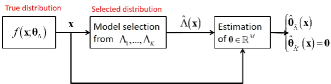
Figure 1: Estimation after model selection: The true pdf that generates the measurement vector, ${\bf{x}}$, is $f({\bf{x}};{\mbox{\boldmath$\theta$}}_{\Lambda})$, where $\Lambda\in\{\Lambda_{k}\}_{k=1}^{K}$ is the true support set, such that $\Lambda_{k}\in{\cal{P}}(\{1,\ldots,M\})$, $k=1,\ldots,K$. In the first processing stage, a model (support set) is selected according to a predetermined selection rule, which results in an estimated support set, $\hat{\Lambda}\in\{\Lambda_{k}\}_{k=1}^{K}$. In the second stage, the full unknown parameter vector, ${\mbox{\boldmath$\theta$}}\in{\mathbb{R}}^{M}$, is estimated based on ${\bf{x}}$ and on $\hat{\Lambda}$, where coherency implies that $\hat{{\mbox{\boldmath$\theta$}}}_{\hat{\Lambda}^{c}}={\bf{0}}$.

The probability of selecting the $k$th model is denoted as

$$\pi_{k}({\mbox{\boldmath$\theta$}}_{\Lambda})\stackrel{{\scriptstyle\triangle}}{{=}}\Pr({\hat{\Lambda}=\Lambda}_{k};{\mbox{\boldmath$\theta$}}_{\Lambda}),~{}k=1,\ldots,K,$$ (2)

where this probability is computed w.r.t. the true pdf, $f({\bf{x}};{\mbox{\boldmath$\theta$}}_{\Lambda})$. We assume that the deterministic sets

$${\mathcal{A}}_{k}\stackrel{{\scriptstyle\triangle}}{{=}}\{{\bf{x}}:{\bf{x}}\in\Omega_{\bf{x}},\hat{\Lambda}({\bf{x}})=\Lambda_{k}\},~{}k=1,\ldots,K,$$ (3)

generate a partition of $\Omega_{\bf{x}}$. That is, $\{{\mathcal{A}}_{k}\}_{k=1}^{K}$ are mutually disjoint subsets of $\Omega_{\bf{x}}$, whose union is $\Omega_{\bf{x}}$. By using Bayes rule, it can be verified that

$$f({\bf{x}}|{\hat{\Lambda}=\Lambda}_{k};{\mbox{\boldmath$\theta$}}_{\Lambda})=\frac{f({\bf{x}};{\mbox{\boldmath$\theta$}}_{\Lambda})}{\pi_{k}({\mbox{\boldmath$\theta$}}_{\Lambda})},~{}\forall{\bf{x}}\in{\mathcal{A}}_{k},$$ (4)

$\forall{\mathcal{A}}_{k}$ such that $\pi_{k}({\mbox{\boldmath$\theta$}}_{\Lambda})\neq 0$. We also define the null parameters that have been wrongly selected by the selection rule.

Definition 2.

A parameter is said to be a null parameter if it does not appear in the true model. Thus, the set of all null parameters is given by ${\mbox{\boldmath$\theta$}}_{\Lambda^{c}}$.

The support sets of the unknown parameter vectors, $\{\Lambda_{k}\}_{k=1}^{K}$, and the true support set, $\Lambda$, differ in size. In order to compare between the estimation errors in different models, we introduce the zero-padded vectors, where the zero-padding is to the length of the full parameter vector, $M$.

Definition 3.

For an arbitrary vector, ${\bf{a}}\in{\mathbb{R}}^{M}$, and any candidate support set, ${\Lambda}_{k}$, $k=1,\ldots,K$, the vector ${\bf{a}}_{{\Lambda}_{k}}^{\text{\tiny{ZP}}}$, is a zero-padded, $M$-length vector, whose non-padded elements correspond to the elements of ${\bf{a}}_{{\Lambda}_{k}}$.

In this paper, we are interested in analyzing the performance of coherent estimators, as defined in Definition 1. Thus, only estimation errors that belong to the estimated (non-padded) parameters are relevant in the resultant zero-padded vector. This definition is based on the considered scheme, in which the selection rule is predetermined, and our goal is to analyze the post-model-selection estimation approach. In particular, it can be verified that for any coherent estimator, as defined in Definition 1, $\hat{{\mbox{\boldmath$\theta$}}}_{\hat{\Lambda}}^{\text{\tiny{ZP}}}=\hat{{\mbox{\boldmath$\theta$}}}$. The following example demonstrates our notations.

Example 1.

Consider a case where there are $M=5$ candidate parameters, i.e. ${\mbox{\boldmath$\theta$}}\in{\mathbb{R}}^{5}$, and the true support set and true parameter vector are $\Lambda=\{1,2,3\}$ and ${\mbox{\boldmath$\theta$}}_{\Lambda}=[\theta_{1},\theta_{2},\theta_{3}]^{T}$, respectively. Let us assume that for a specific realization (i.e. specific observation vector, ${\bf{x}}$), the selection rule results in the estimated support set $\hat{\Lambda}=\{1,3,5\}$. Then, according to Definition 1, any coherent estimator has the form $\hat{{\mbox{\boldmath$\theta$}}}=[\hat{\theta}_{1},0,\hat{\theta}_{3},0,\hat{\theta}_{5}]^{T}$. According to Definition 3, the zero-padded estimation error vector for this case is $\hat{{\mbox{\boldmath$\theta$}}}_{\hat{\Lambda}}^{\text{\tiny{ZP}}}-{\mbox{\boldmath$\theta$}}_{\hat{\Lambda}}^{\text{\tiny{ZP}}}=[\hat{\theta}_{1}-\theta_{1},0,\hat{\theta}_{3}-\theta_{3},0,\hat{\theta}_{5}]^{T}$. Thus, for this observation vector, estimation errors include the influence of estimating the true parameters that have also been selected, $\theta_{1}$ and $\theta_{3}$, as well as the influence of the null parameter, $\theta_{5}$.

We use the following selected-square-error (SSE) matrix cost function:

$${\bf{C}}(\hat{{\mbox{\boldmath$\theta$}}},\hat{\Lambda},{\mbox{\boldmath$\theta$}})\stackrel{{\scriptstyle\triangle}}{{=}}\left(\hat{{\mbox{\boldmath$\theta$}}}_{\hat{\Lambda}}^{\text{\tiny{ZP}}}-{\mbox{\boldmath$\theta$}}_{\hat{\Lambda}}^{\text{\tiny{ZP}}}\right)\left(\hat{{\mbox{\boldmath$\theta$}}}_{\hat{\Lambda}}^{\text{\tiny{ZP}}}-{\mbox{\boldmath$\theta$}}_{\hat{\Lambda}}^{\text{\tiny{ZP}}}\right)^{T}.$$ (5)

The corresponding mean SSE (MSSE) is given by

$${\rm{E}}_{{\mbox{\boldmath{\scriptsize$\theta$}}}_{\Lambda}}\left[{\bf{C}}(\hat{{\mbox{\boldmath$\theta$}}},\hat{\Lambda},{\mbox{\boldmath$\theta$}})\right]={\rm{E}}_{{\mbox{\boldmath{\scriptsize$\theta$}}}_{\Lambda}}\left[\left(\hat{{\mbox{\boldmath$\theta$}}}_{\hat{\Lambda}}^{\text{\tiny{ZP}}}-{\mbox{\boldmath$\theta$}}_{\hat{\Lambda}}^{\text{\tiny{ZP}}}\right)\left(\hat{{\mbox{\boldmath$\theta$}}}_{\hat{\Lambda}}^{\text{\tiny{ZP}}}-{\mbox{\boldmath$\theta$}}_{\hat{\Lambda}}^{\text{\tiny{ZP}}}\right)^{T}\right]\hskip 14.22636pt$$

$$=\sum_{k=1}^{K}\pi_{k}({\mbox{\boldmath$\theta$}}_{\Lambda}){\rm{E}}_{{\mbox{\boldmath{\scriptsize$\theta$}}}_{\Lambda}}\left[(\hat{{\mbox{\boldmath$\theta$}}}_{\Lambda_{k}}^{\text{\tiny{ZP}}}-{\mbox{\boldmath$\theta$}}_{\Lambda_{k}}^{\text{\tiny{ZP}}})(\hat{{\mbox{\boldmath$\theta$}}}_{\Lambda_{k}}^{\text{\tiny{ZP}}}-{\mbox{\boldmath$\theta$}}_{\Lambda_{k}}^{\text{\tiny{ZP}}})^{T}|{\hat{\Lambda}=\Lambda}_{k}\right],$$ (6)

where the last equality is obtained by using (4) and the law of total expectation.

The marginal MSSE on a specific parameter, $\theta_{m}$, is given by the $m$th diagonal element of the MSSE, that is,

$${\rm{E}}_{{\mbox{\boldmath{\scriptsize$\theta$}}}_{\Lambda}}\left[[{\bf{C}}(\hat{{\mbox{\boldmath$\theta$}}},\hat{\Lambda},{\mbox{\boldmath$\theta$}})]_{m,m}\right]\hskip 113.81102pt$$

$$=\sum_{k\in\kappa_{m}}\pi_{k}({\mbox{\boldmath$\theta$}}_{\Lambda}){\rm{E}}_{{\mbox{\boldmath{\scriptsize$\theta$}}}_{\Lambda}}\left[(\hat{\theta}_{m}-\theta_{m})^{2}|{\hat{\Lambda}=\Lambda}_{k}\right],$$ (7)

$\forall m=1,\ldots,M$, where

$$\kappa_{m}\stackrel{{\scriptstyle\triangle}}{{=}}\{k|k=1,\ldots,K,~{}m\in\Lambda_{k}\}$$ (8)

is the set of all the models in which the parameter $m$ is a part of the support set. Similarly, $\kappa_{m}^{c}\stackrel{{\scriptstyle\triangle}}{{=}}\{k|k=1,\ldots,K,~{}m\notin\Lambda_{k}\}$ is the set of indices of all models for which the parameter $\theta_{m}$ is not in the associated support set $\Lambda_{k}$, and, therefore, its value is zero. It can be seen that

$$p_{m}({\mbox{\boldmath$\theta$}}_{\Lambda})\stackrel{{\scriptstyle\triangle}}{{=}}\sum\nolimits_{k\in\kappa_{m}}\pi_{k}({\mbox{\boldmath$\theta$}}_{\Lambda})$$ (9)

is the probability that the parameter $m$ has been selected by the considered selection rule. Thus, by using the law of total expectation, (II) can be written as

$${\rm{E}}_{{\mbox{\boldmath{\scriptsize$\theta$}}}_{\Lambda}}[[{\bf{C}}(\hat{{\mbox{\boldmath$\theta$}}},\hat{\Lambda},{\mbox{\boldmath$\theta$}})]_{m,m}]=p_{m}({\mbox{\boldmath$\theta$}}_{\Lambda}){\rm{E}}_{{\mbox{\boldmath{\scriptsize$\theta$}}}_{\Lambda}}[(\hat{\theta}_{m}-\theta_{m})^{2}|m\in\hat{\Lambda}].$$ (10)

It should be noted that $\theta_{m}=0$ in (II) and (10) for any $m\notin\Lambda$.

It can be seen that the SSE cost function from (5) only takes into account the estimation errors of the elements that are not forced to zero by the selection stage. The rationale behind this cost function is that the estimation errors of the unselected parameters are only determined by the selection rule, and cannot be reduced by any coherent estimator. Thus, designing and analyzing post-model-selection estimators can be done only w.r.t. the estimation errors of the selected parameters that can be controlled. In our preliminary work in [56], we consider a limited SSE cost where the estimation errors taken over the intersection of the true and estimated support. In this paper, the MSSE integrates the estimation errors of all selected parameters, that is, both the true parameters on the support set, $\Lambda$, and the second moment of the null parameters, as defined in Definition 2. The rationale behind also taking into account the influence of the null parameters is since, in practical applications, the MSE of these selected null parameters significantly affects the estimation results, especially in the sense of the bias function. In addition, the estimators of the null parameters affect the estimators of the true parameters. Thus, the correlations between the two types of errors via the matrix cost function (i.e. the off-diagonal terms of the SSE in (5)) should also be taken into consideration. Finally, it can be seen that ignoring the contribution of the null parameters’ estimation errors to the risk function may lead to estimators of the null parameters that can be arbitrarily large, even though these parameters do not belong to the model. Thus, we want to control their MSE via the associated second moments.

III Selective CRB

In this section, a CRB-type lower bound for estimation after model selection is derived. The proposed bound is a lower bound on the MSSE of any coherent estimator, as a function of its selective bias function, where selective unbiasedness is defined in Section III-A by using Lehmann unbiasedness. Section III-B shows the relation between the MSE and the MSSE for coherent estimators as a function of the selective bias. The selective CRB is presented in Section III-C, followed by remarks and special cases in Section III-D. An preliminary derivation of the scalar selective CRB appears in [56].

III-A Selective unbiasedness

In order to exclude trivial estimators, the mean-unbiasedness constraint is commonly used in non-Bayesian parameter estimation [57]. However, this constraint is inappropriate for estimation after model selection, since we are interested only in errors of the selected parameters and since the data-based model selection step induces bias [22]. Lehmann [26] proposed a generalization of the unbiasedness concept based on the considered cost function. In our previous work (p. 13 in [58]) we extended the scalar Lehmann unbiasedness definition to the general case of a matrix cost function, as follows.

Definition 4.

The estimator, $\hat{{\mbox{\boldmath$\theta$}}}$, is said to be a uniformly unbiased estimator of $\theta$ in the Lehmann sense w.r.t. the positive semidefinite matrix cost function, ${\bf{C}}(\hat{{\mbox{\boldmath$\theta$}}},{\mbox{\boldmath$\theta$}})$, if

$${\rm{E}}_{{\mbox{\boldmath{\scriptsize$\theta$}}}}[{\bf{C}}(\hat{{\mbox{\boldmath$\theta$}}},{\mbox{\boldmath$\eta$}})]\succeq{\rm{E}}_{{\mbox{\boldmath{\scriptsize$\theta$}}}}[{\bf{C}}(\hat{{\mbox{\boldmath$\theta$}}},{\mbox{\boldmath$\theta$}})],~{}\forall{\mbox{\boldmath$\eta$}},{\mbox{\boldmath$\theta$}}\in\Omega_{\mbox{\boldmath{\scriptsize$\theta$}}},$$ (11)

where $\Omega_{\mbox{\boldmath{\scriptsize$\theta$}}}$ is the parameter space.

Lehmann unbiasedness conditions for various cost functions can be found in [46, 47, 59, 60, 61]. The following proposition defines a sufficient condition for the selective unbiasedness property of estimators w.r.t. the SSE matrix cost function and the selection rule. To this end, we define the selective bias of the estimator, $\hat{{\mbox{\boldmath$\theta$}}}$, under the selected $k$th model and the selection rule, $\hat{\Lambda}$, as follows:

$${\bf{b}}_{k}({\mbox{\boldmath$\theta$}},\Lambda)\stackrel{{\scriptstyle\triangle}}{{=}}{\rm{E}}_{{\mbox{\boldmath{\scriptsize$\theta$}}}_{\Lambda}}[\hat{{\mbox{\boldmath$\theta$}}}_{\Lambda_{k}}^{\text{\tiny{ZP}}}-{\mbox{\boldmath$\theta$}}_{\Lambda_{k}}^{\text{\tiny{ZP}}}|{\hat{\Lambda}=\Lambda}_{k}],~{}k=1,\ldots,K.$$ (12)

Proposition 1.

If

$${\bf{b}}_{k}({\mbox{\boldmath$\theta$}},\Lambda)={\bf{0}},~{}k=1,\ldots,K,$$ (13)

such that $\pi_{k}({\mbox{\boldmath$\theta$}}_{\Lambda})\neq 0$, then, the estimator $\hat{{\mbox{\boldmath$\theta$}}}$ is an unbiased estimator of $\theta$ in the Lehmann sense w.r.t. the SSE matrix defined in (5) and the selection rule $\hat{\Lambda}$.

Proof:

The proof appears in Appendix A. ∎

It should be noted that the selective unbiasedness is defined as a function of the specific model selection rule. In the following, an estimator, $\hat{{\mbox{\boldmath$\theta$}}}$, is said to be a selective unbiased estimator for the problem of estimating $\theta$ with the support set, $\Lambda$, and a given model selection rule, $\hat{\Lambda}$, if the sufficient condition in (13) is satisfied. However, it should be noted that in practice, coherent post-model-selection estimators tend to be biased, similarly to in various cases of nonlinear estimation problems [62].

The condition in (13) implies the requirement that all the scalar estimators of the elements of $\theta$ satisfy

$${\rm{E}}_{{\mbox{\boldmath{\scriptsize$\theta$}}}_{\Lambda}}[\hat{{\mbox{\boldmath$\theta$}}}_{m}|\hat{\Lambda}=\Lambda_{k}]=\left\{\begin{array}[]{lr}\theta_{m}&k\in\kappa_{m}\\ 0&k\notin\kappa_{m}\end{array}\right.,~{}\forall m=1,\ldots,M,$$ (14)

$\forall{\mbox{\boldmath$\theta$}}\in{\mathbb{R}}^{M}$ and $\Lambda\subseteq\{1,\ldots,M\}$. It should be noted that $\theta_{m}=0$ in (14) for the null parameters. In addition, by multiplying (13) by $\pi_{k}({\mbox{\boldmath$\theta$}}_{\Lambda})$ and summing over the candidate models, $k=1,\ldots,K$, we obtain that the condition in (13) implies, in particular, that $\forall{\mbox{\boldmath$\theta$}}\in{\mathbb{R}}^{M}$, $\Lambda\subseteq\{1,\ldots,M\}$,

$$\sum\nolimits_{k=1}^{K}\pi_{k}({\mbox{\boldmath$\theta$}}_{\Lambda}){\bf{b}}_{k}({\mbox{\boldmath$\theta$}},\Lambda)={\rm{E}}_{{\mbox{\boldmath{\scriptsize$\theta$}}}_{\Lambda}}[\hat{{\mbox{\boldmath$\theta$}}}_{\hat{\Lambda}}^{\text{\tiny{ZP}}}-{\mbox{\boldmath$\theta$}}_{\hat{\Lambda}}^{\text{\tiny{ZP}}}]={\bf{0}}.$$ (15)

III-B Relation between MSE and MSSE

In this subsection we develop the relation between the MSE and MSSE measures for coherent estimators. This relation is used in Subsection III-C for obtaining a lower bound on the MSE of coherent estimators directly from the selective CRB on the MSSE. Let the MSE of any estimator $\hat{{\mbox{\boldmath$\theta$}}}\in{\mathbb{R}}^{M}$ be given by

$${\text{MSE}}(\hat{{\mbox{\boldmath$\theta$}}},{\mbox{\boldmath$\theta$}},\Lambda)\stackrel{{\scriptstyle\triangle}}{{=}}{\rm{E}}_{{\mbox{\boldmath{\scriptsize$\theta$}}}_{\Lambda}}\left[(\hat{{\mbox{\boldmath$\theta$}}}-{\mbox{\boldmath$\theta$}})(\hat{{\mbox{\boldmath$\theta$}}}-{\mbox{\boldmath$\theta$}})^{T}\right].$$ (16)

The following proposition states the relation between the MSE from (16) and the MSSE from (II) for coherent estimators.

Proposition 2.

For any coherent estimator with the selective bias ${\bf{b}}_{k}({\mbox{\boldmath$\theta$}},\Lambda)$, as defined in (12), the MSE satisfies

$${\text{{MSE}}}(\hat{{\mbox{\boldmath$\theta$}}},{\mbox{\boldmath$\theta$}},\Lambda)\hskip 170.71652pt$$

$$={\rm{E}}_{{\mbox{\boldmath{\scriptsize$\theta$}}}_{\Lambda}}\left[{\bf{C}}(\hat{{\mbox{\boldmath$\theta$}}},\hat{\Lambda},{\mbox{\boldmath$\theta$}})\right]+\sum_{k=1}^{K}\pi_{k}({\mbox{\boldmath$\theta$}}_{\Lambda}){{\mbox{\boldmath$\theta$}}}_{\Lambda_{k}^{c}}^{\text{\tiny{ZP}}}({{\mbox{\boldmath$\theta$}}}_{\Lambda_{k}^{c}}^{\text{\tiny{ZP}}})^{T}\hskip 28.45274pt$$

$$-\sum_{k=1}^{K}\pi_{k}({\mbox{\boldmath$\theta$}}_{\Lambda})\left({\mbox{\boldmath$\theta$}}_{\Lambda_{k}^{c}}^{\text{\tiny{ZP}}}{\bf{b}}_{k}^{T}({\mbox{\boldmath$\theta$}},\Lambda)+{\bf{b}}_{k}({\mbox{\boldmath$\theta$}},\Lambda)({\mbox{\boldmath$\theta$}}_{\Lambda_{k}^{c}}^{\text{\tiny{ZP}}})^{T}\right).$$ (17)

Proof:

The proof appears in Appendix B. ∎

That is, the MSE in (2) is the sum of the MSSE, the influence of the selective bias of the estimator, and an additional term, $\sum_{k=1}^{K}\pi_{k}({\mbox{\boldmath$\theta$}}_{\Lambda}){{\mbox{\boldmath$\theta$}}}_{\Lambda_{k}^{c}}^{\text{\tiny{ZP}}}({{\mbox{\boldmath$\theta$}}}_{\Lambda_{k}^{c}}^{\text{\tiny{ZP}}})^{T}$, which is only a function of the selection rule and is not affected by the estimator, $\hat{{\mbox{\boldmath$\theta$}}}$. Therefore, by deriving a CRB-type lower bound on the MSSE we readily obtain a lower bound on the MSE of any coherent estimator with a known selective bias function by using the relation in Proposition 2.

By using the definition in (12), it can be verified that the selective bias can have a nonzero value only on $\Lambda_{k}$, and, thus, it has no overlap with ${\mbox{\boldmath$\theta$}}_{\Lambda_{k}^{c}}$. Therefore, the diagonal elements of ${\mbox{\boldmath$\theta$}}_{\Lambda_{k}^{c}}^{\text{\tiny{ZP}}}{\bf{b}}_{k}^{T}({\mbox{\boldmath$\theta$}},\Lambda)$ satisfy

$$\left[{\mbox{\boldmath$\theta$}}_{\Lambda_{k}^{c}}^{\text{\tiny{ZP}}}{\bf{b}}_{k}^{T}({\mbox{\boldmath$\theta$}},\Lambda)\right]_{m,m}=0,~{}m=1,\ldots,M,$$ (18)

and the trace of the matrix ${\mbox{\boldmath$\theta$}}_{\Lambda_{k}^{c}}^{\text{\tiny{ZP}}}{\bf{b}}_{k}^{T}({\mbox{\boldmath$\theta$}},\Lambda)$ is zero. By applying the trace operator on (2) and then substituting (18), we obtain

$${\text{Tr}}\left({\text{MSE}}(\hat{{\mbox{\boldmath$\theta$}}},{\mbox{\boldmath$\theta$}},\Lambda)\right)={\text{Tr}}\left({\rm{E}}_{{\mbox{\boldmath{\scriptsize$\theta$}}}_{\Lambda}}[{\bf{C}}(\hat{{\mbox{\boldmath$\theta$}}},\hat{\Lambda},{\mbox{\boldmath$\theta$}}_{\Lambda})]\right)$$

$$+\sum_{k=1}^{K}\pi_{k}({\mbox{\boldmath$\theta$}}_{\Lambda}){\text{Tr}}\left({{\mbox{\boldmath$\theta$}}}_{\Lambda_{k}^{c}}^{\text{\tiny{ZP}}}({{\mbox{\boldmath$\theta$}}}_{\Lambda_{k}^{c}}^{\text{\tiny{ZP}}})^{T}\right),$$ (19)

where the last term in (III-B) is only a function of the true parameters, ${\mbox{\boldmath$\theta$}}_{\Lambda}$, since it is assumed that $|\Lambda_{k}|\leq M$ for any candidate model, $k=1,\ldots,K$. Similarly, by substituting (10) in the $m$th diagonal element of the MSE from (2) and using (III-B), we obtain that the marginal MSE on a specific parameter that belongs to the true model, $\theta_{m}$, is given by

$${\rm{E}}_{{\mbox{\boldmath{\scriptsize$\theta$}}}_{\Lambda}}\left[(\hat{\theta}_{m}-\theta_{m})^{2}\right]=\hskip 135.15059pt$$

$$p_{m}({\mbox{\boldmath$\theta$}}_{\Lambda}){\rm{E}}_{{\mbox{\boldmath{\scriptsize$\theta$}}}_{\Lambda}}\left[(\hat{\theta}_{m}-\theta_{m})^{2}|m\in\hat{\Lambda}\right]+\left(1-p_{m}({\mbox{\boldmath$\theta$}}_{\Lambda})\right)\theta_{m}^{2},$$ (20)

$\forall m\in{\Lambda}$, Since $\theta_{m}=0$, $\forall m\in{\Lambda^{c}}$, then, the marginal MSE on a null parameter is

$${\rm{E}}_{{\mbox{\boldmath{\scriptsize$\theta$}}}_{\Lambda}}\left[(\hat{\theta}_{m}-\theta_{m})^{2}\right]=p_{m}({\mbox{\boldmath$\theta$}}_{\Lambda}){\rm{E}}_{{\mbox{\boldmath{\scriptsize$\theta$}}}_{\Lambda}}\left[\hat{\theta}_{m}^{2}|m\in\hat{\Lambda}\right],$$ (21)

$\forall m\in{\Lambda^{c}}$.

III-C Selective CRB

Obtaining the estimator with the minimum MSSE among all coherent estimators with a specific selective bias is usually intractable. Thus, lower bounds on the MSSE and MSE of any coherent estimator are useful for performance analysis and system design. In the following, a novel CRB for estimation after model selection, named here selective CRB, is derived. To this end, we define the following post-model-selection likelihood gradient vectors:

$${\mbox{\boldmath$\upsilon$}}_{k}({\bf{x}},{\mbox{\boldmath$\theta$}}_{\Lambda})\stackrel{{\scriptstyle\triangle}}{{=}}\nabla_{{\mbox{\boldmath{\scriptsize$\theta$}}}_{\Lambda}}^{T}\log f({\bf{x}}|{\hat{\Lambda}=\Lambda}_{k};{\mbox{\boldmath$\theta$}}_{\Lambda}),~{}~{}~{}\forall{\bf{x}}\in{\mathcal{A}}_{k},$$ (22)

for any $k=1,\ldots,K$ such that $\pi_{k}({\mbox{\boldmath$\theta$}}_{\Lambda})\neq 0$. The vectors ${\mbox{\boldmath$\upsilon$}}_{k}({\bf{x}},{\mbox{\boldmath$\theta$}}_{\Lambda})$ are all $|\Lambda|$-dimensional vectors, since the gradient is always w.r.t. the true parameter vector, ${\mbox{\boldmath$\theta$}}_{\Lambda}$. In addition, by substituting (4) in (22) it can be verified that

$${\mbox{\boldmath$\upsilon$}}_{k}({\bf{x}},{\mbox{\boldmath$\theta$}}_{\Lambda})=\nabla_{{\mbox{\boldmath{\scriptsize$\theta$}}}_{\Lambda}}^{T}\log f({\bf{x}};{\mbox{\boldmath$\theta$}}_{\Lambda})-\nabla_{{\mbox{\boldmath{\scriptsize$\theta$}}}_{\Lambda}}^{T}\log\pi_{k}({\mbox{\boldmath$\theta$}}_{\Lambda}),$$ (23)

$\forall{\bf{x}}\in{\mathcal{A}}_{k}$. The marginal selective FIM is defined as

$${\bf{J}}_{k}({\mbox{\boldmath$\theta$}}_{\Lambda})\stackrel{{\scriptstyle\triangle}}{{=}}{\rm{E}}_{{\mbox{\boldmath{\scriptsize$\theta$}}}_{\Lambda}}[{\mbox{\boldmath$\upsilon$}}_{k}({\bf{x}},{\mbox{\boldmath$\theta$}}_{\Lambda}){\mbox{\boldmath$\upsilon$}}_{k}^{T}({\bf{x}},{\mbox{\boldmath$\theta$}}_{\Lambda})|{\hat{\Lambda}=\Lambda}_{k}],$$ (24)

$k=1,\ldots,K$. For any $k=1,\ldots,K$, the ${\bf{D}}_{k}(\Lambda)$ is a $M\times|\Lambda|$ matrix with the elements

$$\left[{\bf{D}}_{k}(\Lambda)\right]_{m,l}\stackrel{{\scriptstyle\triangle}}{{=}}\left\{\begin{array}[]{cc}1,&m\in{\Lambda}_{k},~{}m=[\Lambda]_{l}\\ 0,&{\text{otherwise}}\end{array}\right.,$$ (27)

$\forall l=1,\ldots,M$, where $[\Lambda]_{l}$ denotes the $l$th element of the true support set (not to be confused with the $l$th candidate support set, $\Lambda_{l}$). Finally, the zero-padded gradient of the $k$th selective bias from (12) is defined as

$${\bf{G}}_{k}({\mbox{\boldmath$\theta$}},\Lambda)\stackrel{{\scriptstyle\triangle}}{{=}}\nabla_{{\mbox{\boldmath{\scriptsize$\theta$}}}_{\Lambda}}{\bf{b}}_{k}({\mbox{\boldmath$\theta$}},\Lambda),~{}\forall k=1,\ldots,K.$$ (28)

We assume the following regularity conditions:

1. The post-model-selection likelihood gradient vectors, ${\mbox{\boldmath$\upsilon$}}_{k}({\bf{x}},{\mbox{\boldmath$\theta$}}_{\Lambda})$, $k=1,\ldots,K$, exist, and the selective FIMs, ${\bf{J}}_{k}({\mbox{\boldmath$\theta$}}_{\Lambda})$, $k=1,\ldots,K$, are well-defined and nonsingular matrices, $\forall{\mbox{\boldmath$\theta$}}_{\Lambda}\in{\mathbb{R}}^{|\Lambda|}$.

2. The operations of integration w.r.t. ${\bf{x}}$ and differentiation w.r.t. ${\mbox{\boldmath$\theta$}}_{\Lambda}$ can be interchanged, as follows:

   $$\nabla_{{\mbox{\boldmath{\scriptsize$\theta$}}}_{\Lambda}}\int_{\mathcal{A}_{k}}g({\bf{x}})f({\bf{x}}|{\hat{\Lambda}=\Lambda}_{k};{\mbox{\boldmath$\theta$}}_{\Lambda})\,\mathrm{d}{\bf{x}}\hskip 56.9055pt$$

   $$=\int_{\mathcal{A}_{k}}g({\bf{x}})\nabla_{{\mbox{\boldmath{\scriptsize$\theta$}}}_{\Lambda}}f({\bf{x}}|{\hat{\Lambda}=\Lambda}_{k};{\mbox{\boldmath$\theta$}}_{\Lambda})\,\mathrm{d}{\bf{x}},$$ (29)

   $\forall k=1,\ldots,K$, for any measurable function, $g:\Omega_{{\bf{x}}}\rightarrow{\mathbb{R}}$, $\forall{\mbox{\boldmath$\theta$}}_{\Lambda}\in{\mathbb{R}}^{|\Lambda|}$. Similar to the regularity conditions of the CRB (see, e.g. Chapter 2 in [63]), a sufficient condition for this to hold is that the subset of $\Omega_{\bf{x}}$ given by $\{{\bf{x}}\in\Omega_{\bf{x}}|f({\bf{x}}|{\hat{\Lambda}=\Lambda}_{k};{\mbox{\boldmath$\theta$}}_{\Lambda})>0\}$ is the same $\forall{\mbox{\boldmath$\theta$}}_{\Lambda}$.

The following theorem presents the proposed selective CRB.

Theorem 1.

Let the regularity Conditions C.1-C.2 be satisfied, $\hat{\Lambda}$ be a given selection rule, and $\hat{{\mbox{\boldmath$\theta$}}}$ be a coherent estimator of $\theta$ with the support set, $\Lambda$, where the selective bias of the estimator is ${\bf{b}}_{k}({\mbox{\boldmath$\theta$}},\Lambda)$, as defined in (12). Then, the MSSE satisfies

$${\rm{E}}_{{\mbox{\boldmath{\scriptsize$\theta$}}}_{\Lambda}}[{\bf{C}}(\hat{{\mbox{\boldmath$\theta$}}},\hat{\Lambda},{\mbox{\boldmath$\theta$}})]\succeq{\bf{B}}_{\text{sCRB}}({\mbox{\boldmath$\theta$}}_{\Lambda}),$$ (30)

where the selective CRB is given by

$${\bf{B}}_{\text{sCRB}}({\mbox{\boldmath$\theta$}}_{\Lambda})\hskip 170.71652pt$$

$$\stackrel{{\scriptstyle\triangle}}{{=}}\sum_{k=1}^{K}\pi_{k}({\mbox{\boldmath$\theta$}}_{\Lambda})\left(\Psi_{k}({\mbox{\boldmath$\theta$}},\Lambda)+{\bf{b}}_{k}({\mbox{\boldmath$\theta$}},\Lambda){\bf{b}}_{k}^{T}({\mbox{\boldmath$\theta$}},\Lambda)\right),$$ (31)

in which

$$\Psi_{k}({\mbox{\boldmath$\theta$}},\Lambda)\stackrel{{\scriptstyle\triangle}}{{=}}\hskip 170.71652pt$$

$$({\bf{D}}_{k}(\Lambda)+{\bf{G}}_{k}({\mbox{\boldmath$\theta$}},\Lambda)){\bf{J}}_{k}^{-1}({\mbox{\boldmath$\theta$}}_{\Lambda})({\bf{D}}_{k}(\Lambda)+{\bf{G}}_{k}({\mbox{\boldmath$\theta$}},\Lambda))^{T},$$ (32)

${\bf{D}}_{k}(\Lambda)$ is the zero-one matrix defined in (27), and ${\bf{J}}_{k}({\mbox{\boldmath$\theta$}}_{\Lambda})$ is the $k$th selective FIM, defined in (24). Furthermore, the MSE from (2) is bounded by

$${\text{\em{MSE}}}(\hat{{\mbox{\boldmath$\theta$}}},{\mbox{\boldmath$\theta$}}_{\Lambda})\succeq{\bf{B}}_{\text{sCRB}}({\mbox{\boldmath$\theta$}}_{\Lambda})+\sum_{k=1}^{K}\pi_{k}({\mbox{\boldmath$\theta$}}_{\Lambda}){{\mbox{\boldmath$\theta$}}}_{\Lambda_{k}^{c}}^{\text{\tiny{ZP}}}({{\mbox{\boldmath$\theta$}}}_{\Lambda_{k}^{c}}^{\text{\tiny{ZP}}})^{T}$$

$$-\sum_{k=1}^{K}\pi_{k}({\mbox{\boldmath$\theta$}}_{\Lambda})\left({\mbox{\boldmath$\theta$}}_{\Lambda_{k}^{c}}^{\text{\tiny{ZP}}}{\bf{b}}_{k}^{T}({\mbox{\boldmath$\theta$}},\Lambda)+{\bf{b}}_{k}({\mbox{\boldmath$\theta$}},\Lambda)({\mbox{\boldmath$\theta$}}_{\Lambda_{k}^{c}}^{\text{\tiny{ZP}}})^{T}\right).$$ (33)

Proof:

The proof appears in Appendix C. ∎

The MSE and MSSE bounds in Theorem 1 are matrix bounds. As such, they imply the associated marginal bounds on the diagonal elements and on the trace. That is, by using the $m$th element of the MSSE from (10) and the bound from (30)-(1), we obtain the marginal selective CRB on the MSSE of the $m$th element of $\theta$:

$$p_{m}({\mbox{\boldmath$\theta$}}_{\Lambda}){\rm{E}}_{{\mbox{\boldmath{\scriptsize$\theta$}}}_{\Lambda}}\left[(\hat{\theta}_{m}-\theta_{m})^{2}|m\in\hat{\Lambda}\right]\geq[{\bf{B}}_{\text{sCRB}}({\mbox{\boldmath$\theta$}}_{\Lambda})]_{m,m}$$

$$=\sum_{k\in\kappa_{m}}\pi_{k}({\mbox{\boldmath$\theta$}}_{\Lambda})\left(\left[\Psi_{k}({\mbox{\boldmath$\theta$}},\Lambda)\right]_{m,m}+\left[{\bf{b}}_{k}({\mbox{\boldmath$\theta$}},\Lambda)\right]_{m,m}^{2}\right),$$ (34)

$\forall m=1,\ldots,M$, where $\kappa_{m}$ is defined in (8). Similarly, using the $m$th marginal MSE from (III-B) and the matrix MSE bound from (1) implies the following marginal MSE bounds:

$${\rm{E}}_{{\mbox{\boldmath{\scriptsize$\theta$}}}_{\Lambda}}\left[(\hat{\theta}_{m}-\theta_{m})^{2}\right]\geq\hskip 113.81102pt$$

$$\sum_{k\in\kappa_{m}}\pi_{k}({\mbox{\boldmath$\theta$}}_{\Lambda})\left([\Psi_{k}({\mbox{\boldmath$\theta$}},\Lambda)]_{m,m}+[{\bf{b}}_{k}({\mbox{\boldmath$\theta$}},\Lambda)]_{m,m}^{2}\right)$$

$$+\left(1-p_{m}({\mbox{\boldmath$\theta$}}_{\Lambda})\right)\theta_{m}^{2},\hskip 113.81102pt$$ (35)

$\forall m=1,\ldots,M$, where $p_{m}({\mbox{\boldmath$\theta$}}_{\Lambda})$ is defined in (9). Summing (III-C), over $m=1,\ldots,M$, and using the fact that ${\mbox{\boldmath$\theta$}}_{\Lambda^{c}}={\bf{0}}$, we obtain the associated selective CRB on the trace MSE:

$${\text{Tr}}\left({\text{MSE}}(\hat{{\mbox{\boldmath$\theta$}}},{\mbox{\boldmath$\theta$}}_{\Lambda})\right)\hskip 156.49014pt$$

$$\geq\sum_{m=1}^{M}\sum_{k\in\kappa_{m}}\pi_{k}({\mbox{\boldmath$\theta$}}_{\Lambda})\left([\Psi_{k}({\mbox{\boldmath$\theta$}},\Lambda)]_{m,m}+\left[{\bf{b}}_{k}({\mbox{\boldmath$\theta$}},\Lambda)\right]_{m,m}^{2}\right)$$

$$+\sum\nolimits_{m\in\Lambda}\left(1-p_{m}({\mbox{\boldmath$\theta$}}_{\Lambda})\right)\theta_{m}^{2}.\hskip 99.58464pt$$ (36)

In the following we present the selective CRB for selective unbiased estimators. By substituting (13) in (1), we obtain that for selective unbiased estimators $\Psi_{k}({\mbox{\boldmath$\theta$}},\Lambda)={\bf{D}}_{k}(\Lambda){\bf{J}}_{k}^{-1}({\mbox{\boldmath$\theta$}}_{\Lambda}){\bf{D}}_{k}^{T}(\Lambda),$ and, thus, the selective CRB from (1) is reduced to

$${\bf{B}}_{\text{sCRB}}({\mbox{\boldmath$\theta$}}_{\Lambda})=\sum_{k=1}^{K}\pi_{k}({\mbox{\boldmath$\theta$}}_{\Lambda}){\bf{D}}_{k}(\Lambda){\bf{J}}_{k}^{-1}({\mbox{\boldmath$\theta$}}_{\Lambda}){\bf{D}}_{k}(\Lambda).$$ (37)

Similarly, by substituting (27) and (37) in (III-C), the associated selective CRB on the trace MSE of unbiased selective estimators is reduced to

$${\text{Tr}}\left({\text{MSE}}(\hat{{\mbox{\boldmath$\theta$}}},{\mbox{\boldmath$\theta$}}_{\Lambda})\right)\geq\sum_{l=1}^{|\Lambda|}\sum_{k\in\kappa_{[\Lambda]_{l}}}\pi_{k}({\mbox{\boldmath$\theta$}}_{\Lambda})[{\bf{J}}_{k}^{-1}({\mbox{\boldmath$\theta$}}_{\Lambda})]_{l,l}$$

$$+\sum_{m\in\Lambda}\left(1-p_{m}({\mbox{\boldmath$\theta$}}_{\Lambda})\right)\theta_{m}^{2},\hskip 49.79231pt$$ (38)

where $\kappa_{[\Lambda]_{l}}$ is defined in (8).

It can be seen that for a selective unbiased estimator, as defined in (12), the selective CRB in (37) is a lower bound only on the parameters that belong to the true support set of the vector, $\Lambda$, and does not include the null parameters. Thus, the influence of the selected null parameters (i.e. the parameters that have been wrongly selected by the selection rule) on the estimation of the true parameters is via the selective bias and its gradient, from (12) and (28), respectively. In some applications, it could be useful to take into account only the estimation errors over the intersection of the true and estimated support, i.e. only the values of $\hat{{\mbox{\boldmath$\theta$}}}_{\Lambda\cap\hat{\Lambda}}^{\text{\tiny{ZP}}}-{{\mbox{\boldmath$\theta$}}}_{\Lambda\cap\hat{\Lambda}}^{\text{\tiny{ZP}}}$. In these cases, one can use the unbiased selective CRB from (37) as the lower bound on the MSSE of the true parameters, as appears in our preliminary derivation of the scalar selective CRB in [56].

Finally, the following Lemma presents alternative formulations of the selective FIM that may be more tractable for some estimation problems.

Lemma 1.

Assume that Conditions C.1-C.2 are satisfied in addition to the following regularity conditions:

1. The second-order derivatives of $f({\bf{x}}|{\hat{\Lambda}=\Lambda}_{k};{\mbox{\boldmath$\theta$}}_{\Lambda})$ w.r.t. the elements of ${\mbox{\boldmath$\theta$}}_{\Lambda}$ exist and are bounded and continuous $\forall{\bf{x}}\in\mathcal{A}_{k},~{}k=1,\ldots,K$.

2. The integral, $\int_{\mathcal{A}_{k}}f({\bf{x}}|{\hat{\Lambda}=\Lambda}_{k};{\mbox{\boldmath$\theta$}}_{\Lambda}){\,\mathrm{d}}{\bf{x}}$, is twice differentiable under the integral sign w.r.t. the elements of ${\mbox{\boldmath$\theta$}}_{\Lambda}$, $\forall k=1,\ldots,K$, ${\mbox{\boldmath$\theta$}}_{\Lambda}\in{\mathbb{R}}^{|\Lambda|}$.

Then, the $k$th selective FIM in (24) satisfies

$${\bf{J}}_{k}({\mbox{\boldmath$\theta$}}_{\Lambda})=-{\rm{E}}_{{\mbox{\boldmath{\scriptsize$\theta$}}}_{\Lambda}}\left[\left.\nabla_{{\mbox{\boldmath{\scriptsize$\theta$}}}_{\Lambda}}\nabla_{{\mbox{\boldmath{\scriptsize$\theta$}}}_{\Lambda}}^{T}\log f({\bf{x}};{\mbox{\boldmath$\theta$}}_{\Lambda})\right|{\hat{\Lambda}=\Lambda}_{k}\right]\hskip 8.5359pt$$

$$+\nabla_{{\mbox{\boldmath{\scriptsize$\theta$}}}_{\Lambda}}\nabla_{{\mbox{\boldmath{\scriptsize$\theta$}}}_{\Lambda}}^{T}\log\pi_{k}({\mbox{\boldmath$\theta$}}_{\Lambda}),\hskip 85.35826pt$$ (39)

$$={\rm{E}}_{{\mbox{\boldmath{\scriptsize$\theta$}}}_{\Lambda}}\left[\left.\nabla_{{\mbox{\boldmath{\scriptsize$\theta$}}}_{\Lambda}}^{T}\log f({\bf{x}};{\mbox{\boldmath$\theta$}}_{\Lambda})\nabla_{{\mbox{\boldmath{\scriptsize$\theta$}}}_{\Lambda}}\log f({\bf{x}};{\mbox{\boldmath$\theta$}}_{\Lambda})\right|{\hat{\Lambda}=\Lambda}_{k}\right]$$

$$-\left(\nabla_{{\mbox{\boldmath{\scriptsize$\theta$}}}_{\Lambda}}\log\pi_{k}\left({\mbox{\boldmath$\theta$}}_{\Lambda}\right)\right)^{T}\nabla_{{\mbox{\boldmath{\scriptsize$\theta$}}}_{\Lambda}}\log\pi_{k}\left({\mbox{\boldmath$\theta$}}_{\Lambda}\right),\hskip 42.67912pt$$ (40)

$\forall k=1,\ldots,K$, ${\mbox{\boldmath$\theta$}}_{\Lambda}\in{\mathbb{R}}^{|\Lambda|}$.

Proof:

The proof appears in Appendix D. ∎

III-D Special cases and relation with other CRB-type bounds

III-D1 Single model

When only a single model is assumed, i.e. ${\hat{\Lambda}=\Lambda}_{1}=\Lambda$ and $\pi_{1}({\mbox{\boldmath$\theta$}}_{\Lambda})=1$ for any selection rule, the SSE, selective unbiasedness, and selective CRB are reduced to the MSE, mean-unbiasedness, and CRB for estimating ${\mbox{\boldmath$\theta$}}_{\Lambda}$. Thus, the proposed paradigm generalizes the conventional non-Bayesian parameter estimation.

III-D2 Nested models and the relation to SMS-CRB

A model class is nested if smaller models are always special cases of larger models. Thus, in this special case we assume a model order selection problem in which $\Lambda_{1}\subset\ldots\subset\Lambda_{k_{t}}\ldots\subset\Lambda_{k}$, $\forall k=1,\ldots,K$, where $k_{t}$ is the true model, i.e. $\Lambda=\Lambda_{k_{t}}$. In this special case, the matrix ${\bf{D}}_{k}(\Lambda)$ from (27) is given by

$${\bf{D}}_{k}(\Lambda)=\left\{\begin{array}[]{lr}\begin{bmatrix}{\bf{I}}_{|\Lambda_{k}|}&{\bf{0}}\\ {\bf{0}}&{\bf{0}}\end{bmatrix}&{\text{if }}1\leq k\leq{k_{t}}\\ \begin{bmatrix}{\bf{I}}_{|\Lambda|}\\ {\bf{0}}\end{bmatrix}&{\text{if }}{k_{t}}\leq k\leq K\end{array}\right..$$ (41)

By substituting (41) in the unbiased selective CRB from (37), we obtain

$${\bf{B}}_{\text{sCRB}}({\mbox{\boldmath$\theta$}}_{\Lambda})=\sum_{k=1}^{K}\pi_{k}({\mbox{\boldmath$\theta$}}_{\Lambda})\hskip 113.81102pt$$

$$\times\begin{bmatrix}[{\bf{J}}_{k}^{-1}({\mbox{\boldmath$\theta$}}_{\Lambda})]_{\{1:\min\{|\Lambda_{k}|,\Lambda\},1:\min\{|\Lambda_{k}|,\Lambda\}\}}&{\bf{0}}\\ {\bf{0}}&{\bf{0}}\end{bmatrix},$$ (42)

$\forall k=1,\ldots,K$.

The SMS-CRB bound from [1] was developed for the problem of model order selection with nested models under the assumptions:

1. The order selection rule is such that asymptotically $\Pr({\hat{\Lambda}=\Lambda}_{k};{\mbox{\boldmath$\theta$}}_{\Lambda})=0$, for any $k<k_{t}$. Hence, only overestimation of the order is considered.

2. The FIMs under the $k$th candidate model, defined as

   $$\tilde{{\bf{J}}}_{k}({\mbox{\boldmath$\theta$}}_{\Lambda_{k}})\stackrel{{\scriptstyle\triangle}}{{=}}-{\rm{E}}_{{\mbox{\boldmath{\scriptsize$\theta$}}}_{\Lambda_{k}}}[\nabla_{{\mbox{\boldmath{\scriptsize$\theta$}}}_{\Lambda_{k}}}(\nabla^{T}_{{\mbox{\boldmath{\scriptsize$\theta$}}}_{\Lambda_{k}}}\log f({\bf{x}};{\mbox{\boldmath$\theta$}}_{\Lambda_{k}}))],$$ (43)

   are nonsingular matrices for any $k=1,\ldots,K$.

Under Assumptions A.1-A.2, the SMS-CRB is given by [1]

$${\bf{B}}_{\text{SMS-CRB}}({\mbox{\boldmath$\theta$}})\stackrel{{\scriptstyle\triangle}}{{=}}\sum_{k=k_{t}}^{K}\pi_{k}({\mbox{\boldmath$\theta$}}_{\Lambda}){\bf{F}}_{k}({\mbox{\boldmath$\theta$}}_{\Lambda_{k}})\stackrel{{\scriptstyle\triangle}}{{=}}\begin{bmatrix}\tilde{{\bf{J}}}_{k}^{-1}({\mbox{\boldmath$\theta$}}_{\Lambda_{k}})&{\bf{0}}\\ {\bf{0}}&{\bf{0}}\end{bmatrix}.$$ (44)

It can be seen that the proposed selective CRB for nested models from (III-D2) has a similar structure to the SMS-CRB bound from (44). However, the proposed selective CRB accounts for both overestimation and underestimation of the model order, while the SMS-CRB accounts only for overestimation. The selective CRB is based on a different selective FIM for each model, that takes into account the selection rule, while the SMS-CRB is based on averaging over the FIMs of the different candidate models, as can be seen from comparing (III-D2) and (44). Finally, our bound is not limited to the nested setting and is shown to be tighter than the SMS-CRB in simulations.

III-D3 Data-independent selection rule

In this degenerated case, we consider a random selection rule, which is independent of the data and of its parameters. Thus, the derivative of the log of the probability of selection of the $k$th model w.r.t. ${\mbox{\boldmath$\theta$}}_{\Lambda}$ vanishes:

$$\nabla_{{\mbox{\boldmath{\scriptsize$\theta$}}}_{\Lambda}}^{T}\log\pi_{k}({\mbox{\boldmath$\theta$}}_{\Lambda})={\bf{0}}.$$ (45)

In addition, since the selection is independent of the observation vector, ${\bf{x}}$, then

$$-{\rm{E}}_{{\mbox{\boldmath{\scriptsize$\theta$}}}_{\Lambda}}\left[\left.\nabla_{{\mbox{\boldmath{\scriptsize$\theta$}}}_{\Lambda}}\nabla_{{\mbox{\boldmath{\scriptsize$\theta$}}}_{\Lambda}}^{T}\log f({\bf{x}};{\mbox{\boldmath$\theta$}}_{\Lambda})\right|{\hat{\Lambda}=\Lambda}_{k}\right]={\bf{J}}({\mbox{\boldmath$\theta$}}_{\Lambda}),$$ (46)

$\forall k=1,\ldots,K$, where

$${\bf{J}}({\mbox{\boldmath$\theta$}}_{\Lambda})\stackrel{{\scriptstyle\triangle}}{{=}}-{\rm{E}}_{{\mbox{\boldmath{\scriptsize$\theta$}}}_{\Lambda}}[\nabla_{{\mbox{\boldmath{\scriptsize$\theta$}}}_{\Lambda}}(\nabla^{T}_{{\mbox{\boldmath{\scriptsize$\theta$}}}_{\Lambda}}\log f({\bf{x}};{\mbox{\boldmath$\theta$}}_{\Lambda}))]$$ (47)

is the oracle FIM, which is based on knowledge of the true model. By substituting (45) and (46) in the selective FIM from (1), we obtain that for a random selection rule,

$${\bf{J}}_{k}({\mbox{\boldmath$\theta$}}_{\Lambda})={\bf{J}}({\mbox{\boldmath$\theta$}}_{\Lambda}),~{}\forall k=1,\ldots,K.$$ (48)

Substitution of (48) in the selective CRB from (37), results in

$${\bf{B}}_{\text{sCRB}}({\mbox{\boldmath$\theta$}}_{\Lambda})=\sum_{k=1}^{K}\pi_{k}({\mbox{\boldmath$\theta$}}_{\Lambda}){\bf{D}}_{k}(\Lambda){\bf{J}}^{-1}({\mbox{\boldmath$\theta$}}_{\Lambda}){\bf{D}}_{k}(\Lambda).$$ (49)

Thus, for a random selection rule, the selective CRB is a weighted average over the elements of the oracle CRB, ${\bf{J}}^{-1}({\mbox{\boldmath$\theta$}}_{\Lambda})$, where the weights are defined by the probability of selection.

III-D4 Relation with the misspecified CRB

Estimation after model selection can be interpreted as estimation with a misspecified (or mismatched) model [49, 50, 51, 52, 64], where the true pdf is $f({\bf{x}};\theta_{\Lambda})$ for any ${\bf{x}}\in\Omega_{\bf{x}}$, and the assumed pdf (which may be wrong) is

$$\tilde{f}({\bf{x}};{\mbox{\boldmath$\theta$}})={\text{const}}\times\sum_{k=1}^{K}f({\bf{x}};\theta_{\Lambda_{k}}){\mathbf{1}}_{\{{\bf{x}}\in{\mathcal{A}}_{k}\}},$$ (50)

where “const” is the normalization factor of the pdf. The sets ${\mathcal{A}}_{k}$ are defined in (3) and are associated by the predetermined selection rule, $\hat{\Lambda}$. However, it should be noted that the misspecified CRB in [49, 50, 51, 52] for the considered post-model-selection scheme is a lower bound on ${\rm{E}}_{{\mbox{\boldmath{\scriptsize$\theta$}}}_{\Lambda}}[(\hat{{\mbox{\boldmath$\theta$}}}-{\mbox{\boldmath$\mu$}})(\hat{{\mbox{\boldmath$\theta$}}}-{\mbox{\boldmath$\mu$}})^{T}]$, where ${\mbox{\boldmath$\mu$}}\stackrel{{\scriptstyle\triangle}}{{=}}{\rm{E}}_{{\mbox{\boldmath{\scriptsize$\theta$}}}_{\Lambda}}[\hat{{\mbox{\boldmath$\theta$}}}]$. This risk function can be interpreted as the squared-error of the average selected parameter vector or the estimator, which is different from the SSE cost function in (5). The SSE is more appropriate for evaluating post-model-selection estimation error that aims to be close to the true parameter vector, ${\mbox{\boldmath$\theta$}}_{\Lambda}$. In addition, the misspecified CRB does not take into account the coherency of the estimators, as defined in Definition 1, which is a significant aspect of the considered scheme. These differences are since, in contrast to the misspecified CRB, we consider a well-specified architecture in which the full set of candidate models is known.

III-E Practical implementation of the selective CRB

The proposed selective CRB from Theorem 1, as well as its different versions described in (III-C)-(III-C), requires the calculation of the selection probability, $\pi_{k}({\mbox{\boldmath$\theta$}}_{\Lambda})$, the marginal selective FIM, ${\bf{J}}_{k}({\mbox{\boldmath$\theta$}}_{\Lambda})$, and the gradient of the $k$th selective bias, ${\bf{G}}_{k}({\mbox{\boldmath$\theta$}},\Lambda)$, from (2), (24), and (28), respectively, for each model. When the number of models increases, the efficient evaluation of the probabilities of selection, the selective FIMs, and the bias gradients, is hard. One way to reduce the computational complexity of the proposed bound is by selecting a subset of models and replacing the sum in (1) or (37) by a sum over the subset. This approach is similar to the one used in the Barankin bound [65], in which a set of arbitrary test points is used to compute the bound. The resultant bound is still a valid lower bound, since we only removed non-negative terms that are associated with the neglected models. In order to reduce the set of models and simultaneously to increase the tightness, it intuitively seems more efficient to use the models with the highest probability of selection.
Even after reducing the number of candidate models, the proposed bound may be intractable. In this case, the selective CRB can be approximated by low-complexity methods. Similarly to the empirical FIM in [66, 67], a Monte Carlo approach can be developed to approximate the selective FIMs and the probability of selection by using the stochastic approximation family of algorithms, which results in the empirical selective CRB. The multidimensional integrals needed to calculate the bound are obtained by drawing samples directly from the true distribution, $f\left({\bf{x}};{\mbox{\boldmath$\theta$}}_{\Lambda}\right)$, for a given ${\mbox{\boldmath$\theta$}}_{\Lambda}$, as described, for example, in [68, Ch. 2], or by using Markov chain Monte Carlo (MCMC) samplers [68, Ch. 6]. For example, the probability of selecting the $k$th model from (2) can be written as

$$\pi_{k}\left({\mbox{\boldmath$\theta$}}_{\Lambda}\right)=\int_{\Omega_{\bf{x}}}f\left({\bf{x}};{\mbox{\boldmath$\theta$}}_{\Lambda}\right)\mathbf{1}_{\{{\bf{x}}\in\mathcal{A}_{k}\}}\,\mathrm{d}{\bf{x}}.$$ (51)

Thus, we perform the data generation step as follows: we draw $D$ independent and identically distributed (i.i.d.) samples, $\{\tilde{{\bf{x}}}^{(d)}\}_{d=1}^{D}$, from the true pdf, $f({\bf{x}};{\mbox{\boldmath$\theta$}}_{\Lambda})$. We use these samples in order to approximate (51):

$$\pi_{k}\left({\mbox{\boldmath$\theta$}}_{\Lambda}\right)\approx\frac{1}{D}\sum_{d=1}^{D}\mathbf{1}_{\{\tilde{{\bf{x}}}^{(d)}\in\mathcal{A}_{k}\}}.$$ (52)

From the strong law of large numbers, the approximation in (52) converges almost surely to the probability of selection in (51). Similar approximations can be used for the selective FIM, where the specific structure of the post-model-selection log-likelihood in the selective FIM in its version in (1) makes the calculation tractable, in a similar manner to our derivation in Section IV in [48] for estimation after parameter selection. Then, by replacing the selective FIM and the probability of selection with these approximations in the selective CRB expression from (1) or (37), one can obtain the empirical selective CRB. Due to space limitations, the full details of the empirical selective CRB are not presented in this paper.

IV Sparse vector estimation

In this section, we derive the selective CRB for the special case of estimating an unknown sparse vector, $\theta$, from noisy linear observations. This problem can be formulated as

$${\bf{x}}={\bf{A}}{\mbox{\boldmath$\theta$}}+{\bf{w}}={\bf{A}}_{\Lambda}{\mbox{\boldmath$\theta$}}_{\Lambda}+{\bf{w}},$$ (53)

where ${\bf{A}}\stackrel{{\scriptstyle\triangle}}{{=}}[{\bf{a}}_{1},\ldots,{\bf{a}}_{M}]\in{\mathbb{R}}^{L\times M}$ is a known measurement matrix, whose columns satisfy ${\bf{a}}_{m}^{T}{\bf{a}}_{m}=1$, $\forall m=1,\ldots,M$, and ${\bf{w}}\in{\mathbb{R}}^{L}$ is an independent noise vector. It is assumed that ${\bf{A}}_{\Lambda}$ is a full-rank matrix and that $|\Lambda|\ll M$, i.e. only a small number of elements in the unknown parameter vector, $\theta$, may be nonzero, where the exact sparsity level (size of the support set) is unknown. The candidate models include the different possible support sets of $\theta$, $\Lambda_{k}$, $k=1,\ldots,K$.

Solving model-selection procedures for sparse vector estimation is known to be an NP-hard problem. Thus, we assume the simple selection criterion of one step thresholding (OST) (see, e.g. [69, 70, 71, 72]), which states that

$$m\in\hat{\Lambda}\text{ if }|{\bf{a}}_{m}^{T}{\bf{x}}|>c,~{}\forall m=1,\ldots,M,$$ (54)

where $c$ is a positive, user-selected threshold. This rule simply correlates the observed signal with all the frame vectors and selects the indices where the correlation energy exceeds a certain level, $c$. For the sake of simplicity, we develop the selective CRB for the common setup of additive Gaussian noise. That is, the noise vector, ${\bf{w}}$ from (53), is assumed to be an i.i.d. zero-mean vector with covariance matrix $\sigma^{2}{\bf{I}}_{L}$, where $\sigma^{2}$ is known. We denote the standard normal pdf and cumulative distribution function (cdf) as $\phi(x)\stackrel{{\scriptstyle\triangle}}{{=}}\frac{1}{\sqrt{2\pi}}{\rm{e}}^{-\frac{x^{2}}{2}}$ and $\Phi(x)\stackrel{{\scriptstyle\triangle}}{{=}}\int_{-\infty}^{x}\phi(t){\,\mathrm{d}}t$, respectively. In addition, we use the notations

$$\alpha_{m}\stackrel{{\scriptstyle\triangle}}{{=}}\frac{c-{\bf{a}}_{m}^{T}{\bf{A}}_{\Lambda}{\mbox{\boldmath$\theta$}}_{\Lambda}}{\sigma},~{}m=1,\ldots,M$$ (55)

and

$$\beta_{m}\stackrel{{\scriptstyle\triangle}}{{=}}\frac{-c-{\bf{a}}_{m}^{T}{\bf{A}}_{\Lambda}{\mbox{\boldmath$\theta$}}_{\Lambda}}{\sigma}~{}m=1,\ldots,M.$$ (56)

Theorem 2.

The selective FIM from (24) for the model in (53), where ${\bf{w}}$ is a zero-mean Gaussian vector with a covariance matrix $\sigma^{2}{\bf{I}}_{L}$ and with the OST selection rule, is given by

$${\bf{J}}_{k}({\mbox{\boldmath$\theta$}}_{\Lambda})={\bf{J}}({\mbox{\boldmath$\theta$}}_{\Lambda})+\frac{1}{\sigma^{2}}{\bf{A}}_{\Lambda}^{T}{\bf{Q}}_{k}{\bf{A}}_{\Lambda},$$ (57)

where

$${\bf{J}}({\mbox{\boldmath$\theta$}}_{\Lambda})=\frac{1}{\sigma^{2}}{\bf{A}}_{\Lambda}^{T}{\bf{A}}_{\Lambda}$$ (58)

is the oracle FIM for this case, which is calculated for the true support set of the sparse vector, $\Lambda$, and

$${\bf{Q}}_{k}\stackrel{{\scriptstyle\triangle}}{{=}}\sum_{l\in\Lambda_{k}}{{\bf{a}}_{l}{\bf{a}}_{l}^{T}}\left\{\frac{\phi(\alpha_{l})\alpha_{l}-\phi(\beta_{l})\beta_{l}}{1-\Phi(\alpha_{l})+\Phi(\beta_{l})}\right.\hskip 42.67912pt$$

$$\left.-\frac{\left(\phi(\alpha_{l})-\phi(\beta_{l})\right)^{2}}{\left(1-\Phi(\alpha_{l})+\Phi(\beta_{l})\right)^{2}}\right\}\hskip 64.01869pt$$

$$+\sum_{m\notin\Lambda_{k}}{{\bf{a}}_{m}{\bf{a}}_{m}^{T}}\left\{\frac{-\phi(\alpha_{m})\alpha_{m}+\phi(\beta_{m})\beta_{m}}{\Phi(\alpha_{m})-\Phi(\beta_{m})}\right.$$

$$\left.-\frac{\left(\phi(\alpha_{m})-\phi(\beta_{m})\right)^{2}}{\left(\Phi(\alpha_{m})-\Phi(\beta_{m})\right)^{2}}\right\},\hskip 56.9055pt$$ (59)

for any $k=1,\ldots,K$.

Proof:

The proof appears in Appendix E. ∎

It can be seen that asymptotically, i.e. when $\sigma\rightarrow\infty$, the elements of the matrix ${\bf{Q}}_{k}$ from (2) converge to zero, $\forall k=1,\ldots,K$, faster than those of the oracle FIM from (58). Thus, asymptotically, the selective FIM from (57) converges to the oracle FIM from (58). As a result, in the asymptotic, small-error region the proposed selective CRB and the oracle CRB coincide. However, in the large-error region, while the oracle CRB is known to be non-informative, the selective CRB is an informative lower bound, as shown in the simulations, since it takes into account the probability that the OST selection rule selects wrong parameters and/or misses true parameters.

The selective FIM from Theorem 2 can be used to compute the different versions of the selective CRB from (1) and (1)-(III-C), under the assumption that ${\bf{A}}_{\Lambda}^{T}{\bf{A}}_{\Lambda}+{\bf{A}}_{\Lambda}^{T}{\bf{Q}}_{k}{\bf{A}}_{\Lambda}$, $k=1,\ldots,K$, are nonsingular matrices. In particular, by substituting (114) from Appendix E and (57) in (III-C) we obtain that the selective CRB on the trace MSE of selective unbiased estimators is given by

$${\text{Tr}}\left({\text{MSE}}(\hat{{\mbox{\boldmath$\theta$}}},{\mbox{\boldmath$\theta$}}_{\Lambda})\right)\hskip 142.26378pt$$

$$\geq\sigma^{2}\sum_{l=1}^{|\Lambda|}\sum_{k\in\kappa_{[\Lambda]_{l}}}\pi_{k}({\mbox{\boldmath$\theta$}}_{\Lambda})\left[\left({\bf{A}}_{\Lambda}^{T}\left({\bf{I}}+{\bf{Q}}_{k}\right){\bf{A}}_{\Lambda}\right)^{-1}\right]_{l,l}$$

$$+\sum_{m\in\Lambda}(\Phi(\alpha_{m})-\Phi(\beta_{m}))\theta_{m}^{2},\hskip 71.13188pt$$ (60)

where ${\bf{Q}}_{k}$ is defined in (2), and, according to Appendix E:

$$\pi_{k}({\mbox{\boldmath$\theta$}}_{\Lambda})=\hskip 170.71652pt$$

$$\prod_{l\in\Lambda_{k}}\left(1-\Phi(\alpha_{l})+\Phi(\beta_{l})\right)\prod_{m\notin\Lambda_{k}}\Phi(\alpha_{m})-\Phi(\beta_{m}),$$ (61)

$\forall k=1,\ldots,K$. Since in many sparse estimation scenarios one cannot construct any estimator which is unbiased for all sparsely representable parameters [21], the biased selective CRB from Theorem 1 should be used for cases where the bias gradient of the considered estimator is tractable.

According to Subsection III-E, we can reduce the computational complexity of the bound from (IV)-(IV) by selecting a subset of models such that $k\in\kappa_{m}$, $m\in\Lambda$. It should be noted that the SMS-CRB from (44) cannot be computed for the sparse setting with $L<M$ since the SMS-CRB requires that the FIMs under the $k$th candidate model from (43) will be nonsingular matrices for any $k=1,\ldots,K$, while in the sparse setting these are usually not full-rank matrices.

V Examples

In this section, the proposed selective CRB is evaluated and its performance is compared with that of the SMS-CRB [1] from (44), the oracle CRB, and with the performance of the maximum selected likelihood (MSL) estimator. The MSL estimator is obtained by first choosing a model based on a selection rule and then maximizing the likelihood of the selected model. The performance of the MSL estimator is evaluated using $20,000-100,000$ Monte-Carlo simulations. Unless otherwise noted, in the following simulations we present the unbiased selective CRB from (III-C). Finally, it should be noted that in all simulations the probability of selection is analytically computed.

V-A Example 1 - General linear model

The general linear model is applied to a large set of problems in different fields of science and engineering [73, 74, 75]. Under this model and the $k$th candidate model, the observations obey

$${\bf{x}}={\bf{H}}_{k}{\mbox{\boldmath$\theta$}}_{\Lambda_{k}}+{\bf{w}},$$ (62)

where ${\bf{x}}\in{\mathbb{R}}^{N}$ is the observed vector, the matrices ${\bf{H}}_{k}\in\mathbb{R}^{N\times|\Lambda_{k}|}$, $k=1,\ldots,K$, are assumed to be known full column rank matrices, ${\mbox{\boldmath$\theta$}}\in{\mathbb{R}}^{M}$ is a deterministic unknown vector, and ${\bf{w}}$ is a zero-mean Gaussian random vector with mutually independent elements, each with known variance $\sigma^{2}$.

The coherent MSL estimator, under the assumption that the $k$th model has been selected, is given by (p. 186 in [57])

$$\hat{{\mbox{\boldmath$\theta$}}}^{{\text{ML}}|k}_{\Lambda_{k}}=\left({{\bf{H}}}_{k}^{T}{{\bf{H}}}_{k}\right)^{-1}{{\bf{H}}}_{k}^{T}{\bf{x}},~{}\forall k=1,\ldots,K,$$ (63)

where the other parameters of the MSL estimator are set to zero, i.e. $\hat{{\mbox{\boldmath$\theta$}}}^{{\text{ML}}|k}_{\Lambda_{k}^{c}}={\bf{0}}$, as in (1). The notation $|k$ denotes that the $k$th model was used for the estimation.

We assume here selection rules from the GIC family [4]. For the considered model, the GIC is given by

$$\hat{\Lambda}^{\rm{GIC}}({\bf{x}})=\arg\min_{\Lambda_{1},\ldots,\Lambda_{K}}{\rm{GIC}}(\Lambda_{k},N),$$ (64)

where

$${\rm{GIC}}(\Lambda_{k},N)\stackrel{{\scriptstyle\triangle}}{{=}}-2\log{f({\bf{x}};\hat{{\mbox{\boldmath$\theta$}}}^{{\text{ML}}|k})}+\tau\left(N,|\Lambda_{k}|\right)|\Lambda_{k}|$$ (65)

and $\tau(N,|\Lambda_{k}|)$ is a penalty term. In particular, for the two widely-used AIC and MDL criteria we have

$$\tau\left(N,|\Lambda_{k}|\right)=\left\{\begin{array}[]{ll}2&{\text{AIC}}\\ \log N&{\text{MDL}}\end{array}\right..$$ (66)

By substituting the model from (62) and the $k$th MSL estimator from (63) into (65), and removing constant terms, we obtain

$${\rm{GIC}}(\Lambda_{k},N)=\frac{1}{\sigma^{2}}||{\bf{P}}_{{\bf{H}}_{k}}^{\bot}{\bf{x}}||_{2}^{2}+\tau\left(N,|\Lambda_{k}|\right)|\Lambda_{k}|.$$ (67)

For this model, it can be shown that [57]

$$\nabla_{{\mbox{\boldmath{\scriptsize$\theta$}}}_{\Lambda}}\nabla_{{\mbox{\boldmath{\scriptsize$\theta$}}}_{\Lambda}}^{T}\log f({\bf{x}};{\mbox{\boldmath$\theta$}}_{\Lambda})=-\frac{\tilde{{\bf{H}}}^{T}{\tilde{{\bf{H}}}}}{\sigma^{2}},$$ (68)

where $\tilde{{\bf{H}}}$ is the true measurement matrix, $\tilde{{\bf{H}}}\in\{{\bf{H}}_{k}\}_{k=1}^{K}$. By substituting (68) in (1), it can be verified that, where the correct model is $k$, the selective FIMs are

$$\mathbf{J}_{k}({\mbox{\boldmath$\theta$}})=\frac{\tilde{{\bf{H}}}^{T}\tilde{{\bf{H}}}}{\sigma^{2}}+\nabla_{{\mbox{\boldmath{\scriptsize$\theta$}}}_{\Lambda}}(\nabla^{T}_{{\mbox{\boldmath{\scriptsize$\theta$}}}_{\Lambda}}\log\pi_{k}({\mbox{\boldmath$\theta$}}_{\Lambda})),~{}k=1,\ldots,K.$$ (69)

In general, the probability of selection, $\pi_{k}({\mbox{\boldmath$\theta$}}_{\Lambda})$, does not have an analytical form. For the sake of simplicity, in the following simulations we set $K=2$, ${\bf{H}}_{1}={\bf{h}}_{1}$, and ${\bf{H}}_{2}=[{\bf{h}}_{1},{\bf{h}}_{2}]$. Thus, $\Lambda_{1}=\{1\}$, $\Lambda_{2}=\{1,2\}$, ${\mbox{\boldmath$\theta$}}_{\Lambda_{1}}=\theta_{1}$, ${\mbox{\boldmath$\theta$}}_{\Lambda_{2}}={\mbox{\boldmath$\theta$}}\in{\mathbb{R}}^{2}$. We simulate data where $k=2$ is the true model, i.e. ${\mbox{\boldmath$\theta$}}_{\Lambda}={\mbox{\boldmath$\theta$}}$. Thus, in this case there are no null parameters that have been wrongly selected, and the influence of the selection rule is via the coherency property from (1). This situation arises in many real-world scenarios with non-synthetic data and with no real null parameters. According to (67) and by using some algebraic manipulations, the probability of selecting the $k=2$ model is

$$\pi_{2}({\mbox{\boldmath$\theta$}})=\Pr\left(-\frac{1}{\sigma^{2}}{\bf{x}}^{T}({\bf{P}}_{{\bf{H}}_{2}}^{\bot}-{\bf{P}}_{{\bf{H}}_{1}}^{\bot}){\bf{x}}\geq\gamma;{\mbox{\boldmath$\theta$}}\right)$$ (70)

$$=Q_{\frac{1}{2}}(\sqrt{\lambda},\sqrt{\gamma}),\hskip 103.85237pt$$ (71)

where $\gamma\stackrel{{\scriptstyle\triangle}}{{=}}2\tau(N,2)-\tau(N,1)$, $\lambda=\frac{\theta_{2}^{2}}{\sigma^{2}}\frac{||{\bf{h}}_{1}||_{2}^{2}||{\bf{h}}_{2}||_{2}^{2}-({\bf{h}}_{1}^{T}{\bf{h}}_{2})^{2}}{||{\bf{h}}_{1}||_{2}^{2}}$, and $Q_{m}(\cdot,\cdot)$ is the general Marcum Q-function of order $m$. The probability in (71) is obtained by using the fact that $-\frac{1}{\sigma^{2}}{\bf{x}}^{T}({\bf{P}}_{{\bf{H}}_{2}}^{\bot}-{\bf{P}}_{{\bf{H}}_{1}}^{\bot}){\bf{x}}$ has a noncentral $\chi$-squared distribution with 1 degree of freedom and a non-centrality parameter $\lambda$ (see, e.g. [76]). Since $\pi_{2}({\mbox{\boldmath$\theta$}})$ is only a function of $\theta_{2}$, the only nonzero element of $\nabla_{{\mbox{\boldmath{\scriptsize$\theta$}}}_{\Lambda}}(\nabla^{T}_{{\mbox{\boldmath{\scriptsize$\theta$}}}_{\Lambda}}\log\pi_{2}({\mbox{\boldmath$\theta$}}))$ from (69) is its $(2,2)$th element, which satisfies

$$\left[\nabla_{{\mbox{\boldmath{\scriptsize$\theta$}}}_{\Lambda}}(\nabla^{T}_{{\mbox{\boldmath{\scriptsize$\theta$}}}_{\Lambda}}\log\pi_{2}({\mbox{\boldmath$\theta$}}))\right]_{2,2}=\frac{\partial^{2}\log\pi_{2}({\mbox{\boldmath$\theta$}})}{\partial\theta_{2}^{2}}\hskip 49.79231pt$$

$$=-\frac{1}{(\pi_{2}({\mbox{\boldmath$\theta$}}))^{2}}\left(\frac{\partial\pi_{2}({\mbox{\boldmath$\theta$}})}{\partial\theta_{2}}\right)^{2}+\frac{1}{\pi_{2}({\mbox{\boldmath$\theta$}})}\frac{\partial^{2}\pi_{2}({\mbox{\boldmath$\theta$}})}{\partial\theta_{2}^{2}}.$$ (72)

Similarly, since $\pi_{1}({\mbox{\boldmath$\theta$}})=1-\pi_{2}({\mbox{\boldmath$\theta$}})$, the only nonzero element of $\nabla_{{\mbox{\boldmath{\scriptsize$\theta$}}}_{\Lambda}}(\nabla^{T}_{{\mbox{\boldmath{\scriptsize$\theta$}}}_{\Lambda}}\log\pi_{1}({\mbox{\boldmath$\theta$}}))$ is its $(2,2)$th element, which satisfies

$$\left[\nabla_{{\mbox{\boldmath{\scriptsize$\theta$}}}_{\Lambda}}(\nabla^{T}_{{\mbox{\boldmath{\scriptsize$\theta$}}}_{\Lambda}}\log\pi_{1}({\mbox{\boldmath$\theta$}}))\right]_{2,2}=\hskip 106.69783pt$$

$$-\frac{1}{(1-\pi_{2}({\mbox{\boldmath$\theta$}}))^{2}}\left(\frac{\partial\pi_{2}({\mbox{\boldmath$\theta$}})}{\partial\theta_{2}}\right)^{2}-\frac{1}{1-\pi_{2}({\mbox{\boldmath$\theta$}})}\frac{\partial^{2}\pi_{2}({\mbox{\boldmath$\theta$}})}{\partial\theta_{2}^{2}}.$$ (73)

The closed-form expressions of (V-A) and (V-A) are obtained by realizing that [77]

$$\frac{\partial}{\partial\theta_{2}}\pi_{2}({\mbox{\boldmath$\theta$}})=\frac{\lambda}{\theta_{2}}\left(Q_{\frac{3}{2}}(\sqrt{\lambda},\sqrt{\gamma})-Q_{\frac{1}{2}}(\sqrt{\lambda},\sqrt{\gamma})\right)$$ (74)

and

$$\frac{\partial^{2}}{\partial\theta_{2}^{2}}\pi_{2}({\mbox{\boldmath$\theta$}})=-\frac{\lambda}{\theta_{2}^{2}}\left(Q_{\frac{3}{2}}(\sqrt{\lambda},\sqrt{\gamma})-Q_{\frac{1}{2}}(\sqrt{\lambda},\sqrt{\gamma})\right)$$

$$+\frac{\lambda^{2}}{\theta_{2}^{2}}\left(Q_{\frac{5}{2}}(\sqrt{\lambda},\sqrt{\gamma})-2Q_{\frac{3}{2}}(\sqrt{\lambda},\sqrt{\gamma})+Q_{\frac{1}{2}}(\sqrt{\lambda},\sqrt{\gamma})\right).$$ (75)

Based on the Gaussian pdf and (71), it can be shown, similarly to in Appendix E, that the function $f({\bf{x}}|{\hat{\Lambda}=\Lambda}_{k};{\mbox{\boldmath$\theta$}}_{\Lambda})$ is smooth in the sense that its first- and second-order derivatives are well defined. The associated second-order derivatives appear in (68), (V-A), and (V-A). In addition, based on the considered model and (4), the support of the conditional pdf, $f({\bf{x}}|{\hat{\Lambda}=\Lambda}_{k};{\mbox{\boldmath$\theta$}}_{\Lambda})$, is $\mathbb{R}^{N}$ for all ${\mbox{\boldmath$\theta$}}_{\Lambda}$, which implies that Condition C.2 is satisfied. Thus, Conditions C.1-C.4 are satisfied for the considered model as long as the selective FIMs are nonsingular matrices, as required in Condition C.1. By substituting (70)-(V-A) in (69) and then substituting the result in (37), we obtain that the selective CRB for this case is given by

$${\bf{B}}_{\text{sCRB}}({\mbox{\boldmath$\theta$}})=\left[\begin{array}[]{cc}\pi_{1}({\mbox{\boldmath$\theta$}})[{\bf{J}}_{1}^{-1}({\mbox{\boldmath$\theta$}})]_{1,1}&0\\ 0&0\end{array}\right]+\pi_{2}({\mbox{\boldmath$\theta$}}){\bf{J}}_{2}^{-1}({\mbox{\boldmath$\theta$}}),$$ (78)

where

$$\mathbf{J}_{k}({\mbox{\boldmath$\theta$}})=\frac{1}{\sigma^{2}}{{\bf{H}}_{2}}^{T}{{\bf{H}}_{2}}+\left[\begin{array}[]{cc}0&0\\ 0&\frac{\partial^{2}\log\pi_{k}({\mbox{\boldmath{\scriptsize$\theta$}}})}{\partial\theta_{2}^{2}}\end{array}\right],~{}k=1,2.$$ (81)

Finally, by using the definition in (9), it can be seen that $p_{1}({\mbox{\boldmath$\theta$}})=1$ and $p_{2}({\mbox{\boldmath$\theta$}})=\pi_{2}({\mbox{\boldmath$\theta$}})$. Thus, the selective CRB on the trace MSE of selective unbiased estimators from (III-C) for this case is given by

$${\text{Tr}}\left({\text{MSE}}(\hat{{\mbox{\boldmath$\theta$}}},{\mbox{\boldmath$\theta$}}_{\Lambda})\right)\geq\hskip 135.15059pt$$

$$\pi_{1}({\mbox{\boldmath$\theta$}})[{\bf{J}}_{1}^{-1}({\mbox{\boldmath$\theta$}})]_{1,1}+\pi_{2}({\mbox{\boldmath$\theta$}})\sum_{m=1}^{2}[{\bf{J}}_{2}^{-1}({\mbox{\boldmath$\theta$}})]_{m,m}+\pi_{1}({\mbox{\boldmath$\theta$}})\theta_{2}^{2},$$ (82)

under the assumption that ${\bf{J}}_{1}({\mbox{\boldmath$\theta$}})$ and ${\bf{J}}_{2}({\mbox{\boldmath$\theta$}})$ are nonsingular matrices. This assumption held for all tested scenarios.

First, we show the results for the AIC model selection rule, i.e. where $\tau\left(N,|\Lambda_{k}|\right)=2$ in (67). The selective CRB from (V-A), the trace of the SMS-CRB from [1], and the trace of the oracle CRB for the $k=2$ model are evaluated and compared to the MSE of the MSL estimator, where the selection of the likelihood is based on the AIC criterion, versus signal-to-noise ratio (SNR) and versus $\pi_{2}({\mbox{\boldmath$\theta$}})$ in Figs. 2.a and 2.b, respectively. The SNR is defined as ${\rm{SNR}}\stackrel{{\scriptstyle\triangle}}{{=}}10\log 10\frac{||{\bf{H}}{\mbox{\boldmath{\scriptsize$\theta$}}}||^{2}}{N\sigma^{2}}$, where $N=1,500$ samples, ${\mbox{\boldmath$\theta$}}=[4,-3]^{T}$, ${\bf{h}}_{1}=[1,\ldots,1]^{T}$, and the values of ${\bf{h}}_{2}$ are randomly drawn from a uniform distribution in the interval $[0,10]$. It can be seen that the oracle CRB is not a valid bound on the MSE of the MSL estimator for low SNRs, in contrast to the selective CRB and the SMS-CRB. Moreover, the proposed selective CRB is tighter than the SMS-CRB and, in this example, can predict the “breakdown phenomena”, i.e. the threshold region where the MSE of the MSL estimator deviates from the oracle CRB. This breakdown means that the estimator makes gross, anomalous errors with a high probability [45], where in this case these errors are in the model selection phase.

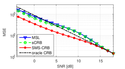
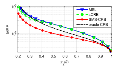
Figure 2: General linear model with AIC selection rule: the MSE of the MSL estimator, the selective CRB, the SMS-CRB, and the oracle CRB, versus SNR (a) and versus the probability of selection of the true model, $\pi_{2}({\mbox{\boldmath$\theta$}})$ (b).

In Fig. 3 we examined these bounds and the performance of the MSL estimator for different values of the GIC penalty term, $\tau(N,|\Lambda_{k}|)$, from (67), ranging from $\tau(N,|\Lambda_{k}|)=2$, associated with the AIC, to $\tau(N,|\Lambda_{k}|)=\log N$, associated with the MDL, for $N=150$ and SNR$=-3.5,0$dB. The oracle CRB is a constant for any penalty, $\tau(N,|\Lambda_{k}|)$; thus, it is inappropriate for post-model-selection estimation. Moreover, the SMS-CRB decreases as $\tau(N,|\Lambda_{k}|)$ increases, in contrast to the MSE of the MSL estimator. This is since the assumptions of the SMS-CRB (Assumptions A.1-A.2) do not hold in this case. It can be seen that the selective CRB is tighter than the SMS-CRB and the oracle CRB in all examined scenarios, but it is less tight as $\tau(N,|\Lambda_{k}|)$ increases. The gap between the selective CRB and the MSE of the MSL estimator may suggest that better post-model-selection estimators can be derived, such as conditional ML estimators [36, 47, 48]. Since in this figure we present only the MSE of the correct parameters, the penalty on overestimation is not presented in this figure. Since the AIC tends to overestimate the order of the model, the MSL estimator of the likelihood selected by the AIC rule has a lower MSE than the MSL estimator of the likelihood selected by the MDL rule. As a result, the selective CRB is tighter with the AIC selection rule than with the MDL selection rule. This is in line with previous observations: “the behavior of AIC with respect to the probability of correct detection is not entirely satisfactory. Interestingly, it is precisely this kind of behavior that appears to make AIC perform satisfactorily with respect to the other possible type of performance measure” [4].

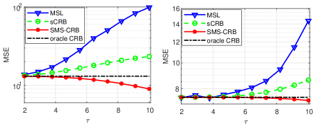
Figure 3: General linear model with GIC selection rule: The MSE of the MSL estimator, the selective CRB, and the SMS-CRB, versus different values of the parameter $\tau(N,|\Lambda_{k}|)$, with SNR$=-3.5$dB (left) and $0$dB (right).

V-B Example 2 - Sparse vector estimation

In this subsection, we demonstrate the use of the selective CRB for measuring the achievable MSE in the sparse estimation problem from Section IV. We validate in simulations the assumption that the matrices ${\bf{A}}_{\hat{\Lambda}}^{T}{\bf{A}}_{\hat{\Lambda}}$, and ${\bf{A}}_{\hat{\Lambda}}^{T}{\bf{A}}_{\hat{\Lambda}}+{\bf{A}}_{\Lambda}^{T}{\bf{Q}}_{k}{\bf{A}}_{\Lambda}$, $k=1,\ldots,K$, are nonsingular matrices. The ML sparse estimator is computationally prohibitive when the dimensions are large [21], and, thus, cannot be used in practice. The coherent MSL estimator, which maximizes the likelihood selected by the OST selection rule for this model, is given by (see, e.g. [21])

$$\hat{{\mbox{\boldmath$\theta$}}}^{{\text{ML|OST}}}_{\hat{\Lambda}}=\left({\bf{A}}_{\hat{\Lambda}}^{T}{\bf{A}}_{\hat{\Lambda}}\right)^{-1}{\bf{A}}_{\hat{\Lambda}}^{T}{\bf{x}},$$ (83)

where $\hat{\Lambda}$ is the estimated support set by the OST rule, defined in (54). The other parameters of this estimator are set to zero, i.e. $\hat{{\mbox{\boldmath$\theta$}}}^{{\text{ML|OST}}}_{\hat{\Lambda}^{c}}={\bf{0}}$. Thus, according to (1), the MSL is a coherent estimator. In order to have a fair comparison with the oracle CRB, the results in this subsection are the MSE of the true parameters, ${\rm{E}}_{{\mbox{\boldmath{\scriptsize$\theta$}}}_{\Lambda}}[(\hat{{\mbox{\boldmath$\theta$}}}_{\Lambda}-{\mbox{\boldmath$\theta$}}_{\Lambda})(\hat{{\mbox{\boldmath$\theta$}}}_{\Lambda}-{\mbox{\boldmath$\theta$}}_{\Lambda})^{T}]$. Similarly, the bounds in these figures are on the submatrix of the MSE of the true parameters.

First, we generate a random $7\times 14$ dictionary, ${\bf{A}}$, from a zero-mean Gaussian i.i.d. distribution, whose columns ${\bf{a}}_{m}$ were normalized so that ${\bf{a}}_{m}^{T}{\bf{a}}_{m}$=1, $m=1,\ldots,M$, where $M=14$ and the mutual coherence of the chosen matrix [17], which is the maximum absolute value of the normalized inner product between the columns of the matrix, was $\mu=0.5673$. We choose a support set uniformly at random, set ${\mbox{\boldmath$\theta$}}_{\Lambda}={\mathbf{1}}$, and change the value of $\sigma^{2}$ to obtain different SNR values. The OST selection rule (54) is implemented with $c=0.95$ as a threshold. The MSE of the true parameters of the MSL estimator from (83) is compared with the selective CRB for sparse estimation, computed by using the selective FIM from Theorem 2 in Fig. 4 for a support set size of $|\Lambda|=3$ and different noise variances, $\sigma^{2}$. It can be seen that the MSE of the MSL estimator and the proposed selective CRB converge asymptotically to the oracle CRB. Moreover, for this scenario, the selective CRB is a tight and valid bound on the performance of the MSL estimator and it predicts the “breakdown phenomena”. This is since it uses the accurate probability of selection and since in this case asymptotically, the OST chooses the correct model. In contrast, the oracle CRB is not an informative bound in the non-asymptotic region and does not predict the threshold. The SMS-CRB cannot be calculated for this case since it requires that the FIM will be a nonsingular matrix for any model, which is not the case in general sparse estimation. A discussion on the insights behind the behavior of the proposed selective CRB and the influence of the selection probability appears in Subsection V-C.

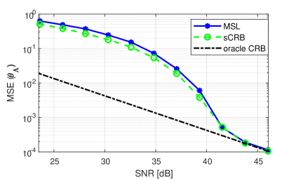
Figure 4: Sparse vector estimation: The MSE of the MSL estimator, where the likelihood is selected by the OST rule, the selective CRB, and the oracle CRB, versus SNR.

Since for general sparse representation problems the MSL estimator is not a selective-unbiased estimator, the proposed selective CRB may not be tight for the general case and, in some cases, may be even higher than the actual MSE. Thus, in the following, we demonstrate the use of the biased selective CRB from (1) for this case, with ${\bf{A}}={\bf{I}}$ and $L=M$. For this case, by substituting (83) and (54) in (12) and using the independency of the elements of the noise vector, ${\bf{w}}$, from (53), we obtain that the $m$th element of the selective bias of the MSL estimator, under the selected $k$th model, is

$$[{\bf{b}}_{k}({\mbox{\boldmath$\theta$}},\Lambda)]_{m} = {\rm{E}}_{{\mbox{\boldmath{\scriptsize$\theta$}}}_{\Lambda}}\left[\left.x_{m}-\theta_{m}\right||x_{m}|>c\right]$$ (84)

$$= -\sigma\frac{\phi(\beta_{m})-\phi(\alpha_{m})}{1-\Phi(\alpha_{m})+\Phi(\beta_{m})},$$

$\forall k=1,\ldots,K$, such that $m\in\Lambda_{k}$, where, according to (55) and (56), in this case $\alpha_{m}=\frac{c-\theta_{m}}{\sigma}$ and $\beta_{m}=\frac{-c-\theta_{m}}{\sigma}$, $\forall m=1,\ldots,M$. The last equality in (84) is obtained by using known results on the moments of truncated Gaussian distributions [78], as well as (114) from Appendix E. In addition, $[{\bf{b}}_{k}({\mbox{\boldmath$\theta$}},\Lambda)]_{m}=0$, $\forall k=1,\ldots,K$, such that $m\in\Lambda_{k}^{c}$. By substituting (84) in (28), we obtain that the elements of the bias gradient matrix are

$$[{\bf{G}}_{k}({\mbox{\boldmath$\theta$}},\Lambda)]_{m,l}=-\sigma\frac{\partial}{\partial\theta_{m}}\frac{\phi(\beta_{m})-\phi(\alpha_{m})}{1-\Phi(\alpha_{m})+\Phi(\beta_{m})}$$

$$=-\frac{\beta_{m}\phi(\beta_{m})-\alpha_{m}\phi(\alpha_{m})}{1-\Phi(\alpha_{m})+\Phi(\beta_{m})}-\frac{1}{\sigma^{2}}([{\bf{b}}_{k}({\mbox{\boldmath$\theta$}},\Lambda)]_{m})^{2},$$ (85)

for any $m\in\Lambda_{k}$, such that $m=[\Lambda]_{l}$, and zero otherwise. By substituting (57) and (V-B) in (1), we obtain the biased CRB for this case. We also evaluate the performance of the iterative post-selection conditional ML (CML) from [36] for this case. Here we use a single iteration and initialize the CML estimator by $\hat{{\mbox{\boldmath$\theta$}}}^{{\text{ML|OST}}}_{\hat{\Lambda}}$. The biased selective CRB for the CML estimator was evaluated numerically, by calculating the selective bias and its gradient, as defined in (12) and (28).

The MSE of the MSL and the CML, as well as the selective CRB, the biased selective CRBs, and the SMS-CRB, are shown in Fig. 5 for varying threshold values, $c$, $K=3$, $M=L=8$, and for two scenarios: 1) ${\mbox{\boldmath$\theta$}}_{\Lambda}=1,~{}\sigma=0.4$; and 2) ${\mbox{\boldmath$\theta$}}_{\Lambda}=0.5,~{}\sigma=1.2$. We denote the biased selective CRB associated with the bias of the MSL estimator by ${\text{b}}_{1}$-sCRB and the biased selective CRB associated with the bias of the CML estimator by ${\text{b}}_{2}$-sCRB. It can be seen that for Scenario 1, the selective CRB is higher than the MSE of the MSL, while for Scenario 2 it is lower than the MSE of the MSL, but is not tight. The performance of the biased selective CRB, ${\text{b}}_{1}$-sCRB, coincides with the performance of the MSL estimator. Similarly, the performance of the biased selective CRB, ${\text{b}}_{2}$-sCRB, almost coincides with the performance of the CML estimator. In contrast to the oracle CRB, which does not show the influence of the threshold parameter, $c$, on the performance, the selective CRB bounds are informative and demonstrate similar patterns (w.r.t. $c$) to the MSE of the estimators. It can be seen that the MSE of the CML estimator is closer to the (unbiased) selective CRB, which may be explained by the results from [36] that show that the CML has a lower selective bias compared with those of the MSL estimator. The SMS-CRB is not shown here since it is significantly lower than the other bounds and since it is also not a valid bound in many tested cases.

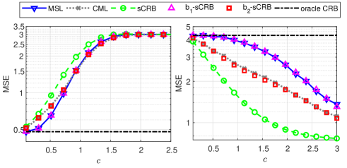
Figure 5: Sparse vector estimation: The MSE of the MSL and of the CML estimators, where the likelihood is selected by the OST rule, the selective CRB, the biased selective CRB with the MSL bias, ${\text{b}}_{1}$-sCRB, the biased selective CRB with the CML bias, ${\text{b}}_{2}$-sCRB, and the oracle CRB, versus the threshold, $c$, for 1) $\theta_{m}=1,\sigma=0.4$ (left); 2) $\theta_{m}=0.5,\sigma=1.2$ (right).

V-C Discussion

It is well known that the threshold effect in the MSE of estimators in nonlinear models is due to large error contributions to the total MSE [25, 65, 45]. In the context of post-model-selection estimation, large errors can be interpreted as the errors due to the incorrect model selection, including both true parameters that are estimated as zero parameters and the wrong selection of null parameters. The small/local errors can be interpreted as the errors due to the estimation approach, when the model selection approaches the true selection. For example, if we look at the selective CRB in (III-C), the influence of the large errors due to the preliminary selection approach is expressed through the following aspects: 1) the term $\sum_{m\in\Lambda}\left(1-p_{m}({\mbox{\boldmath$\theta$}}_{\Lambda})\right)\theta_{m}^{2}$, which is a large-error term, associated with true parameters that are missed by the selection rule; 2) the bias term, ${\bf{b}}_{k}({\mbox{\boldmath$\theta$}},\Lambda)$, which represents large errors for the elements associated with the null parameters; and 3) the selective FIM, ${\bf{J}}_{k}({\mbox{\boldmath$\theta$}}_{\Lambda})$, which, as shown in Lemma 1, includes the influence of the second-order derivatives of the probability of selecting the $k$th model, $\pi_{k}({\mbox{\boldmath$\theta$}}_{\Lambda})$, which is a large-error measure that is sensitive to the selection stage.

Different system parameters affect the ability of the proposed selective CRB to predict the threshold in estimation after model selection problems, which is due to the model selection stage. For example, in Fig. 3 it can be seen that the tightness is different for different selection rules. Another example is for the sparse vector estimation from Subsection V-B; our results (not shown here) indicate that the mutual coherence of ${\bf{A}}$ affects the tightness of the proposed bound, where the selective CRB is less tight as the mutual coherence increases. This is reasonable, since the mutual coherence is used as a measure of the ability of suboptimal algorithms to correctly identify the true representation of a sparse signal. Intuitively, In the extreme case when two columns are completely coherent, it will be impossible to distinguish between their contributions and, thus, impossible to recover the sparse signal, $\theta$. In contrast to the selective CRB, the oracle CRB cannot predict the threshold which is due to the selection, since it does not take into account the coherency property of estimators, nor the preliminary selection stage and the uncertainty in the model. Similarly, the SMS-CRB from (44) cannot predict the threshold since it is developed under Assumption A.1 that there is no underestimation of the order, i.e. the probability that a true parameter has not been selected goes to zero.

VI Conclusion

In this paper, we consider non-Bayesian parameter estimation after model selection. The selection of a model is interpreted here as estimating the selected parameters under a zero constraint on the unselected parameters. First, the notation of selective unbiasedness is defined by using Lehmann’s concept of unbiasedness. We propose a novel Cram$\acute{\text{e}}$r-Rao-type bound, denoted by selective CRB, which is a lower bound on the MSSE of any coherent and selective unbiased estimator. The selective CRB is used also to obtain a lower bound on the MSE of coherent estimators. The relation between the proposed selective CRB and existing bounds, the SMS-CRB and the misspecified CRB, are investigated. The selective CRB was derived for the special case of sparse vector estimation, where the recovery of the support set is performed based on the OST selection rule. In simulations, we have demonstrated that the proposed selective CRB provides an informative bound on the MSL estimator, while the oracle CRB is not a valid bound for this case. Moreover, the proposed selective CRB is tighter than the SMS-CRB (when it exists), and, in some cases, it predicts the breakdown phenomena of the MSL estimator. The predictive capability is attributed to the fact that the selective CRB takes into account the influence of large errors caused by incorrect model selection and the coherency constraint. Our experimental results show that the tightness of the proposed selective CRB depends on the selection rule, on the threshold of the selection rule, and on the measurement matrix.

Topics for future research include the derivation of post-model-selection estimators in the sense of reduced bias, lower MSE, and achievability of the proposed selective CRB, as well as through analysis of the performance (bias and MSE) of the estimators of the null parameters. In addition, the selective CRB may be extended for a Bayesian selection rule and misspecified models [49, 50, 51, 52, 64]. The development of MSE approximations by the method of interval errors [79, 43, 44] could shed more light on the MSE regions of performance and on the threshold phenomenon. Finally, low-complexity bound approximations, such as an empirical CRB, should be developed for cases with intractable probability of selection.

VII ACKNOWLEDGEMENT

The authors would like to thank the anonymous reviewers for their valuable comments. In particular, based on the review process, we extended the SSE cost function from [56] to also include also the influence of the null parameters.

Appendix A Proof of Proposition 1

In this appendix, we prove that the selective unbiasedness is obtained from the Lehmann unbiasedness with the SSE cost function. By substituting (5) in (11), we obtain that the Lehmann unbiasedness for the SSE cost function requires that

$${\rm{E}}_{{\mbox{\boldmath{\scriptsize$\theta$}}}_{\Lambda}}\left[(\hat{{\mbox{\boldmath$\theta$}}}_{\hat{\Lambda}}^{\text{\tiny{ZP}}}-{\mbox{\boldmath$\eta$}}_{\hat{\Lambda}}^{\text{\tiny{ZP}}})(\hat{{\mbox{\boldmath$\theta$}}}_{\hat{\Lambda}}^{\text{\tiny{ZP}}}-{\mbox{\boldmath$\eta$}}_{\hat{\Lambda}}^{\text{\tiny{ZP}}})^{T}\right]\hskip 56.9055pt$$

$$\succeq{\rm{E}}_{{\mbox{\boldmath{\scriptsize$\theta$}}}_{\Lambda}}\left[(\hat{{\mbox{\boldmath$\theta$}}}_{\hat{\Lambda}}^{\text{\tiny{ZP}}}-{\mbox{\boldmath$\theta$}}_{\hat{\Lambda}}^{\text{\tiny{ZP}}})(\hat{{\mbox{\boldmath$\theta$}}}_{\hat{\Lambda}}^{\text{\tiny{ZP}}}-{\mbox{\boldmath$\theta$}}_{\hat{\Lambda}}^{\text{\tiny{ZP}}})^{T}\right],$$ (86)

$\forall{\mbox{\boldmath$\eta$}},{\mbox{\boldmath$\theta$}}\in{\mathbb{R}}^{M}$, where ${\mbox{\boldmath$\theta$}}_{\Lambda^{c}}={\bf{0}}$. By using (4) and the law of total expectation, (A) can be rewritten as

$$\sum\limits_{k=1}^{K}\pi_{k}({\mbox{\boldmath$\theta$}}_{\Lambda}){\rm{E}}_{{\mbox{\boldmath{\scriptsize$\theta$}}}_{\Lambda}}\left[(\hat{{\mbox{\boldmath$\theta$}}}_{\Lambda_{k}}^{\text{\tiny{ZP}}}-{\mbox{\boldmath$\eta$}}_{\Lambda_{k}}^{\text{\tiny{ZP}}})(\hat{{\mbox{\boldmath$\theta$}}}_{\Lambda_{k}}^{\text{\tiny{ZP}}}-{\mbox{\boldmath$\eta$}}_{\Lambda_{k}}^{\text{\tiny{ZP}}})^{T}|{\hat{\Lambda}=\Lambda}_{k}\right]$$

$$\succeq\sum\limits_{k=1}^{K}\pi_{k}({\mbox{\boldmath$\theta$}}_{\Lambda}){\rm{E}}_{{\mbox{\boldmath{\scriptsize$\theta$}}}_{\Lambda}}\left[(\hat{{\mbox{\boldmath$\theta$}}}_{\Lambda_{k}}^{\text{\tiny{ZP}}}-{\mbox{\boldmath$\theta$}}_{\Lambda_{k}}^{\text{\tiny{ZP}}})(\hat{{\mbox{\boldmath$\theta$}}}_{\Lambda_{k}}^{\text{\tiny{ZP}}}-{\mbox{\boldmath$\theta$}}_{\Lambda_{k}}^{\text{\tiny{ZP}}})^{T}|{\hat{\Lambda}=\Lambda}_{k}\right],$$ (87)

By adding and subtracting

$${\bf{u}}_{k}({\mbox{\boldmath$\theta$}}_{\Lambda})\stackrel{{\scriptstyle\triangle}}{{=}}{\rm{E}}_{{\mbox{\boldmath{\scriptsize$\theta$}}}_{\Lambda}}[\hat{{\mbox{\boldmath$\theta$}}}_{\hat{\Lambda}}^{\text{\tiny{ZP}}}|{\hat{\Lambda}=\Lambda}_{k}]={\rm{E}}_{{\mbox{\boldmath{\scriptsize$\theta$}}}_{\Lambda}}[\hat{{\mbox{\boldmath$\theta$}}}_{{\Lambda}_{k}}^{\text{\tiny{ZP}}}|{\hat{\Lambda}=\Lambda}_{k}]$$ (88)

inside the two brackets associated with the $k$th model on both sides of (A) for any $k=1,\ldots,K$, we obtain

$$\sum\limits_{k=1}^{K}\pi_{k}({\mbox{\boldmath$\theta$}}_{\Lambda}){\rm{E}}_{{\mbox{\boldmath{\scriptsize$\theta$}}}_{\Lambda}}\left[\left(\hat{{\mbox{\boldmath$\theta$}}}_{{\Lambda}_{k}}^{\text{\tiny{ZP}}}-{\bf{u}}_{k}({\mbox{\boldmath$\theta$}}_{\Lambda})+{\bf{u}}_{k}({\mbox{\boldmath$\theta$}}_{\Lambda})-{\mbox{\boldmath$\eta$}}_{{\Lambda}_{k}}^{\text{\tiny{ZP}}}\right)\right.$$

$$\left.\times\left(\hat{{\mbox{\boldmath$\theta$}}}_{{\Lambda}_{k}}^{\text{\tiny{ZP}}}-{\bf{u}}_{k}({\mbox{\boldmath$\theta$}}_{\Lambda})+{\bf{u}}_{k}({\mbox{\boldmath$\theta$}}_{\Lambda})-{\mbox{\boldmath$\eta$}}_{{\Lambda}_{k}}^{\text{\tiny{ZP}}}\right)^{T}|{\hat{\Lambda}=\Lambda}_{k}\right]$$

$$\succeq\sum\limits_{k=1}^{K}\pi_{k}({\mbox{\boldmath$\theta$}}_{\Lambda}){\rm{E}}_{{\mbox{\boldmath{\scriptsize$\theta$}}}_{\Lambda}}\left[\left(\hat{{\mbox{\boldmath$\theta$}}}_{{\Lambda}_{k}}^{\text{\tiny{ZP}}}-{\bf{u}}_{k}({\mbox{\boldmath$\theta$}}_{\Lambda})+{\bf{u}}_{k}({\mbox{\boldmath$\theta$}}_{\Lambda})-{\mbox{\boldmath$\theta$}}_{{\Lambda}_{k}}^{\text{\tiny{ZP}}}\right)\right.$$

$$\left.\times\left(\hat{{\mbox{\boldmath$\theta$}}}_{{\Lambda}_{k}}^{\text{\tiny{ZP}}}-{\bf{u}}_{k}({\mbox{\boldmath$\theta$}}_{\Lambda})+{\bf{u}}_{k}({\mbox{\boldmath$\theta$}}_{\Lambda})-{\mbox{\boldmath$\theta$}}_{{\Lambda}_{k}}^{\text{\tiny{ZP}}}\right)^{T}|{\hat{\Lambda}=\Lambda}_{k}\right],$$ (89)

$\forall{\mbox{\boldmath$\eta$}},{\mbox{\boldmath$\theta$}}\in{\mathbb{R}}^{M}$. First, we note that we can remove the identical terms,

$$\sum\limits_{k=1}^{K}\pi_{k}({\mbox{\boldmath$\theta$}}_{\Lambda}){\rm{E}}_{{\mbox{\boldmath{\scriptsize$\theta$}}}_{\Lambda}}\left[(\hat{{\mbox{\boldmath$\theta$}}}_{{\Lambda}_{k}}^{\text{\tiny{ZP}}}-{\bf{u}}_{k}({\mbox{\boldmath$\theta$}}_{\Lambda}))(\hat{{\mbox{\boldmath$\theta$}}}_{{\Lambda}_{k}}^{\text{\tiny{ZP}}}-{\bf{u}}_{k}({\mbox{\boldmath$\theta$}}_{\Lambda}))^{T}|{\hat{\Lambda}=\Lambda}_{k}\right],$$ (90)

from the two sides of (A). In addition, by using (88), it can be verified that

$${\rm{E}}_{{\mbox{\boldmath{\scriptsize$\theta$}}}_{\Lambda}}\left[(\hat{{\mbox{\boldmath$\theta$}}}_{{\Lambda}_{k}}^{\text{\tiny{ZP}}}-{\bf{u}}_{k}({\mbox{\boldmath$\theta$}}_{\Lambda}))({\bf{u}}_{k}({\mbox{\boldmath$\theta$}}_{\Lambda})-{\mbox{\boldmath$\eta$}}_{{\Lambda}_{k}}^{\text{\tiny{ZP}}})^{T}|{\hat{\Lambda}=\Lambda}_{k}\right]={\bf{0}},$$ (91)

$\forall k=1,\ldots,K$. Thus, by subtracting (90) from the two sides of (A) and substituting (91), we obtain that (A) can be rewritten as

$$\sum\limits_{k=1}^{K}\pi_{k}({\mbox{\boldmath$\theta$}}_{\Lambda})\left({\bf{u}}_{k}({\mbox{\boldmath$\theta$}}_{\Lambda})-{\mbox{\boldmath$\eta$}}_{{\Lambda}_{k}}^{\text{\tiny{ZP}}}\right)\left({\bf{u}}_{k}({\mbox{\boldmath$\theta$}}_{\Lambda})-{\mbox{\boldmath$\eta$}}_{{\Lambda}_{k}}^{\text{\tiny{ZP}}}\right)^{T}\hskip 21.33955pt$$

$$\succeq\sum\limits_{k=1}^{K}\pi_{k}\left({\bf{u}}_{k}({\mbox{\boldmath$\theta$}}_{\Lambda})-{\mbox{\boldmath$\theta$}}_{{\Lambda}_{k}}^{\text{\tiny{ZP}}}\right)\left({\bf{u}}_{k}({\mbox{\boldmath$\theta$}}_{\Lambda})-{\mbox{\boldmath$\theta$}}_{{\Lambda}_{k}}^{\text{\tiny{ZP}}}\right)^{T},$$ (92)

$\forall{\mbox{\boldmath$\eta$}},{\mbox{\boldmath$\theta$}}\in{\mathbb{R}}^{M}$.

Now, we note that by using (88), we obtain that the term on the r.h.s. of (A)

$${\bf{u}}_{k}({\mbox{\boldmath$\theta$}}_{\Lambda})-{\mbox{\boldmath$\theta$}}_{{\Lambda}_{k}}^{\text{\tiny{ZP}}}={\rm{E}}_{{\mbox{\boldmath{\scriptsize$\theta$}}}_{\Lambda}}[\hat{{\mbox{\boldmath$\theta$}}}_{\hat{\Lambda}}^{\text{\tiny{ZP}}}-{\mbox{\boldmath$\theta$}}_{\hat{\Lambda}}^{\text{\tiny{ZP}}}|{\hat{\Lambda}=\Lambda}_{k}]={\bf{b}}_{k}({\mbox{\boldmath$\theta$}},\Lambda),$$ (93)

where the last equality is obtained by substituting (12). By substituting (93) in (A), we obtain that the unbiasedness condition can be written as

$$\sum\limits_{k=1}^{K}\pi_{k}({\mbox{\boldmath$\theta$}}_{\Lambda})({\bf{u}}_{k}({\mbox{\boldmath$\theta$}}_{\Lambda})-{\mbox{\boldmath$\eta$}}_{{\Lambda}_{k}}^{\text{\tiny{ZP}}})({\bf{u}}_{k}({\mbox{\boldmath$\theta$}}_{\Lambda})-{\mbox{\boldmath$\eta$}}_{{\Lambda}_{k}}^{\text{\tiny{ZP}}})^{T}\hskip 28.45274pt$$

$$\succeq\sum\limits_{k=1}^{K}\pi_{k}{\bf{b}}_{k}({\mbox{\boldmath$\theta$}},\Lambda){\bf{b}}_{k}^{T}({\mbox{\boldmath$\theta$}},\Lambda),$$ (94)

$\forall{\mbox{\boldmath$\eta$}},{\mbox{\boldmath$\theta$}}\in{\mathbb{R}}^{M}$. Due to the non-negativity of the probabilities, $\pi_{k}({\mbox{\boldmath$\theta$}}_{\Lambda})$, $k=1,\ldots,K$, and of the matrices on the l.h.s. of (A) (in the sense of positive semidefiniteness), the l.h.s. of (A) is necessarily a positive semidefinite matrix. Therefore, a sufficient condition for (A) to hold is if (13) holds.

It should be noted that if the Lehmann condition in (A) must only be satisfied for $\eta$ with the same support set as $\theta$, i.e. for $\eta$ with ${\mbox{\boldmath$\eta$}}_{\Lambda^{c}}={\bf{0}}$, then we will get a less restrictive selective unbiasedness condition. In particular, in Proposition 1 in [56] the selective unbiasedness only restricts the values that are in the intersection of the true and estimated support, i.e. it only restricts the values of $\hat{{\mbox{\boldmath$\theta$}}}_{\Lambda\cap\hat{\Lambda}}$.

Appendix B Proof of Proposition 2

By using Definition 3, the estimation error, $\hat{{\mbox{\boldmath$\theta$}}}-{\mbox{\boldmath$\theta$}}$, can be decomposed w.r.t. the selected support set, $\hat{\Lambda}$, and its complementary, $\hat{\Lambda}^{c}$, as follows:

$$\hat{{\mbox{\boldmath$\theta$}}}-{\mbox{\boldmath$\theta$}}=\hat{{\mbox{\boldmath$\theta$}}}_{\hat{\Lambda}}^{\text{\tiny{ZP}}}-{\mbox{\boldmath$\theta$}}_{\hat{\Lambda}}^{\text{\tiny{ZP}}}+\hat{{\mbox{\boldmath$\theta$}}}_{\hat{\Lambda}^{c}}^{\text{\tiny{ZP}}}-{\mbox{\boldmath$\theta$}}_{\hat{\Lambda}^{c}}^{\text{\tiny{ZP}}},$$ (95)

where all the vectors in (95) have the same dimension, $M$. By substituting (II) and (95) in the MSE matrix from (16), one obtains

$${\text{MSE}}(\hat{{\mbox{\boldmath$\theta$}}},{\mbox{\boldmath$\theta$}},\Lambda)={\rm{E}}_{{\mbox{\boldmath{\scriptsize$\theta$}}}_{\Lambda}}\left[{\bf{C}}(\hat{{\mbox{\boldmath$\theta$}}},\hat{\Lambda},{\mbox{\boldmath$\theta$}}_{\Lambda})\right]\hskip 56.9055pt$$

$$+{\rm{E}}_{{\mbox{\boldmath{\scriptsize$\theta$}}}_{\Lambda}}\left[\left(\hat{{\mbox{\boldmath$\theta$}}}_{\hat{\Lambda}^{c}}^{\text{\tiny{ZP}}}-{\mbox{\boldmath$\theta$}}_{\hat{\Lambda}^{c}}^{\text{\tiny{ZP}}}\right)\left(\hat{{\mbox{\boldmath$\theta$}}}_{\hat{\Lambda}}^{\text{\tiny{ZP}}}-{\mbox{\boldmath$\theta$}}_{\hat{\Lambda}}^{\text{\tiny{ZP}}}\right)^{T}\right]\hskip 9.95863pt$$

$$+{\rm{E}}_{{\mbox{\boldmath{\scriptsize$\theta$}}}_{\Lambda}}\left[\left(\hat{{\mbox{\boldmath$\theta$}}}_{\hat{\Lambda}}^{\text{\tiny{ZP}}}-{\mbox{\boldmath$\theta$}}_{\hat{\Lambda}}^{\text{\tiny{ZP}}}\right)\left(\hat{{\mbox{\boldmath$\theta$}}}_{\hat{\Lambda}^{c}}^{\text{\tiny{ZP}}}-{\mbox{\boldmath$\theta$}}_{\hat{\Lambda}^{c}}^{\text{\tiny{ZP}}}\right)^{T}\right]\hskip 9.95863pt$$

$$+{\rm{E}}_{{\mbox{\boldmath{\scriptsize$\theta$}}}_{\Lambda}}\left[\left(\hat{{\mbox{\boldmath$\theta$}}}_{\hat{\Lambda}^{c}}^{\text{\tiny{ZP}}}-{\mbox{\boldmath$\theta$}}_{\hat{\Lambda}^{c}}^{\text{\tiny{ZP}}}\right)\left(\hat{{\mbox{\boldmath$\theta$}}}_{\hat{\Lambda}^{c}}^{\text{\tiny{ZP}}}-{\mbox{\boldmath$\theta$}}_{\hat{\Lambda}^{c}}^{\text{\tiny{ZP}}}\right)^{T}\right].$$ (96)

The coherency property from (1) after a zero-padding approach, implies that $\hat{{\mbox{\boldmath$\theta$}}}_{\hat{\Lambda}^{c}}^{\text{\tiny{ZP}}}={\bf{0}}$. By substituting $\hat{{\mbox{\boldmath$\theta$}}}_{\hat{\Lambda}^{c}}^{\text{\tiny{ZP}}}={\bf{0}}$ in (B), we obtain that for any coherent estimator, the MSE satisfies

$${\text{MSE}}(\hat{{\mbox{\boldmath$\theta$}}},{\mbox{\boldmath$\theta$}}_{\Lambda})={\rm{E}}_{{\mbox{\boldmath{\scriptsize$\theta$}}}_{\Lambda}}\left[{\bf{C}}(\hat{{\mbox{\boldmath$\theta$}}},\hat{\Lambda},{\mbox{\boldmath$\theta$}}_{\Lambda})\right]\hskip 78.24507pt$$

$$-{\rm{E}}_{{\mbox{\boldmath{\scriptsize$\theta$}}}_{\Lambda}}\left[{\mbox{\boldmath$\theta$}}_{\hat{\Lambda}^{c}}^{\text{\tiny{ZP}}}\left(\hat{{\mbox{\boldmath$\theta$}}}_{\hat{\Lambda}}^{\text{\tiny{ZP}}}-{\mbox{\boldmath$\theta$}}_{\hat{\Lambda}}^{\text{\tiny{ZP}}}\right)^{T}\right]-{\rm{E}}_{{\mbox{\boldmath{\scriptsize$\theta$}}}_{\Lambda}}\left[\left(\hat{{\mbox{\boldmath$\theta$}}}_{\hat{\Lambda}}^{\text{\tiny{ZP}}}-{\mbox{\boldmath$\theta$}}_{\hat{\Lambda}}^{\text{\tiny{ZP}}}\right)\left({\mbox{\boldmath$\theta$}}_{\hat{\Lambda}^{c}}^{\text{\tiny{ZP}}}\right)^{T}\right]$$

$$+{\rm{E}}_{{\mbox{\boldmath{\scriptsize$\theta$}}}_{\Lambda}}\left[{\mbox{\boldmath$\theta$}}_{\hat{\Lambda}^{c}}^{\text{\tiny{ZP}}}\left({\mbox{\boldmath$\theta$}}_{\hat{\Lambda}^{c}}^{\text{\tiny{ZP}}}\right)^{T}\right].\hskip 142.26378pt$$ (97)

Now, by using the law of total expectation, it can be seen that for any coherent and selective biased estimator, the second term on the r.h.s. of (B) satisfies

$${\rm{E}}_{{\mbox{\boldmath{\scriptsize$\theta$}}}_{\Lambda}}\left[{{\mbox{\boldmath$\theta$}}}_{\hat{\Lambda}^{c}}^{\text{\tiny{ZP}}}\left(\hat{{\mbox{\boldmath$\theta$}}}_{\hat{\Lambda}}^{\text{\tiny{ZP}}}-{\mbox{\boldmath$\theta$}}_{\hat{\Lambda}}^{\text{\tiny{ZP}}}\right)^{T}\right]\hskip 85.35826pt$$

$$=\sum_{k=1}^{K}\pi_{k}({\mbox{\boldmath$\theta$}}_{\Lambda}){{\mbox{\boldmath$\theta$}}}_{\Lambda_{k}^{c}}^{\text{\tiny{ZP}}}{\rm{E}}_{{\mbox{\boldmath{\scriptsize$\theta$}}}_{\Lambda}}\left[(\hat{{\mbox{\boldmath$\theta$}}}_{{\Lambda}_{k}}^{\text{\tiny{ZP}}}-{\mbox{\boldmath$\theta$}}_{{\Lambda}_{k}}^{\text{\tiny{ZP}}})^{T}|{\hat{\Lambda}=\Lambda}_{k}\right]$$

$$=\sum_{k=1}^{K}\pi_{k}({\mbox{\boldmath$\theta$}}_{\Lambda}){{\mbox{\boldmath$\theta$}}}_{\Lambda_{k}^{c}}^{\text{\tiny{ZP}}}{{\bf{b}}_{k}^{T}({\mbox{\boldmath$\theta$}},\Lambda}),\hskip 68.28644pt$$ (98)

where the last equality is obtained by substituting the selection bias property from (12). Similarly, by using the law of total expectation, the last term of the r.h.s. of (B) satisfies

$${\rm{E}}_{{\mbox{\boldmath{\scriptsize$\theta$}}}_{\Lambda}}\left[{{\mbox{\boldmath$\theta$}}}_{\hat{\Lambda}^{c}}^{\text{\tiny{ZP}}}({{\mbox{\boldmath$\theta$}}}_{\hat{\Lambda}^{c}}^{\text{\tiny{ZP}}})^{T}\right]=\sum_{k=1}^{K}\pi_{k}({\mbox{\boldmath$\theta$}}_{\Lambda}){{\mbox{\boldmath$\theta$}}}_{\Lambda_{k}^{c}}^{\text{\tiny{ZP}}}({{\mbox{\boldmath$\theta$}}}_{\Lambda_{k}^{c}}^{\text{\tiny{ZP}}})^{T}.$$ (99)

By substituting (B) and (99) in (B) we obtain that the MSE of a coherent and selective unbiased estimator is given by (2).

Appendix C Proof of Theorem 1

By using Conditions C.1 and C.2, it can be shown, similarly to in the proof of Lemma 2.5.3 in [80] for the unconditional likelihood function, that

$${\rm{E}}_{{\mbox{\boldmath{\scriptsize$\theta$}}}_{\Lambda}}\left[{\mbox{\boldmath$\upsilon$}}_{k}^{T}({\bf{x}},{\mbox{\boldmath$\theta$}}_{\Lambda})|{\hat{\Lambda}=\Lambda}_{k}\right]\hskip 85.35826pt$$

$$={\rm{E}}_{{\mbox{\boldmath{\scriptsize$\theta$}}}_{\Lambda}}\left[\nabla_{{\mbox{\boldmath{\scriptsize$\theta$}}}_{\Lambda}}\log f({\bf{x}}|{\hat{\Lambda}=\Lambda}_{k};{\mbox{\boldmath$\theta$}}_{\Lambda})|{\hat{\Lambda}=\Lambda}_{k}\right]={\bf{0}},$$ (100)

$\forall k=1,\ldots,K$ and for any ${\mbox{\boldmath$\theta$}}_{\Lambda}\in\mathbb{R}^{|\Lambda|}$, where ${\mbox{\boldmath$\upsilon$}}_{k}({\bf{x}},{\mbox{\boldmath$\theta$}}_{\Lambda})$ is defined in (22). In addition, for any square-integrable function, ${\mbox{\boldmath$\xi$}}:\Omega_{{\bf{x}}}\times\Omega_{{\mbox{\boldmath{\scriptsize$\theta$}}}}\rightarrow{\mathbb{R}^{M}}$, the covariance inequality (see, e.g. p. 33 in [79]) implies that

$${\rm{E}}_{{\mbox{\boldmath{\scriptsize$\theta$}}}_{\Lambda}}\left[{\mbox{\boldmath$\xi$}}({\bf{x}},{\mbox{\boldmath$\theta$}}){\mbox{\boldmath$\xi$}}^{T}({\bf{x}},{\mbox{\boldmath$\theta$}})\right]\succeq{\rm{E}}_{{\mbox{\boldmath{\scriptsize$\theta$}}}_{\Lambda}}\left[{\mbox{\boldmath$\xi$}}({\bf{x}},{\mbox{\boldmath$\theta$}}){\mbox{\boldmath$\upsilon$}}_{k}^{T}({\bf{x}},{\mbox{\boldmath$\theta$}}_{\Lambda})\right]\hskip 11.38092pt$$

$$\times{\bf{J}}_{k}^{-1}({\mbox{\boldmath$\theta$}}_{\Lambda}){\rm{E}}_{{\mbox{\boldmath{\scriptsize$\theta$}}}_{\Lambda}}\left[{\mbox{\boldmath$\upsilon$}}_{k}({\bf{x}},{\mbox{\boldmath$\theta$}}_{\Lambda}){\mbox{\boldmath$\xi$}}^{T}({\bf{x}},{\mbox{\boldmath$\theta$}})\right],$$ (101)

where, according to Condition C.1, the selective FIMs, ${\bf{J}}_{k}({\mbox{\boldmath$\theta$}}_{\Lambda})$, $k=1,\ldots,K$, are nonsingular matrices, and, thus, (C) is well defined. By substituting ${\mbox{\boldmath$\xi$}}({\bf{x}},{\mbox{\boldmath$\theta$}})=\hat{{\mbox{\boldmath$\theta$}}}_{\Lambda_{k}}^{\text{\tiny{ZP}}}-{\mbox{\boldmath$\theta$}}_{\Lambda_{k}}^{\text{\tiny{ZP}}}-{\bf{b}}_{k}({\mbox{\boldmath$\theta$}},{\Lambda})$ in (C), we obtain

$${\rm{E}}_{{\mbox{\boldmath{\scriptsize$\theta$}}}_{\Lambda}}\left[(\hat{{\mbox{\boldmath$\theta$}}}_{\Lambda_{k}}^{\text{\tiny{ZP}}}-{\mbox{\boldmath$\theta$}}_{\Lambda_{k}}^{\text{\tiny{ZP}}}-{\bf{b}}_{k}({\mbox{\boldmath$\theta$}},{\Lambda}))\right.\hskip 56.9055pt$$

$$\left.\times(\hat{{\mbox{\boldmath$\theta$}}}_{\Lambda_{k}}^{\text{\tiny{ZP}}}-{\mbox{\boldmath$\theta$}}_{\Lambda_{k}}^{\text{\tiny{ZP}}}-{\bf{b}}_{k}({\mbox{\boldmath$\theta$}},{\Lambda}))^{T}|{\hat{\Lambda}=\Lambda}_{k}\right]$$

$$\succeq{\bf{\Lambda}}_{k}({\mbox{\boldmath$\theta$}}_{\Lambda}){\bf{J}}_{k}^{-1}({\mbox{\boldmath$\theta$}}_{\Lambda}){\bf{\Lambda}}_{k}^{T}({\mbox{\boldmath$\theta$}}_{\Lambda}),\hskip 28.45274pt$$ (102)

where

$${\bf{\Lambda}}_{k}({\mbox{\boldmath$\theta$}}_{\Lambda})\hskip 192.05609pt$$

$$\stackrel{{\scriptstyle\triangle}}{{=}}{\rm{E}}_{{\mbox{\boldmath{\scriptsize$\theta$}}}_{\Lambda}}\left[\left(\hat{{\mbox{\boldmath$\theta$}}}_{\Lambda_{k}}^{\text{\tiny{ZP}}}-{\mbox{\boldmath$\theta$}}_{\Lambda_{k}}^{\text{\tiny{ZP}}}-{\bf{b}}_{k}({\mbox{\boldmath$\theta$}},{\Lambda})\right){\mbox{\boldmath$\upsilon$}}_{k}^{T}({\bf{x}},{\mbox{\boldmath$\theta$}}_{\Lambda})|{\hat{\Lambda}=\Lambda}_{k}\right]$$

$$={\rm{E}}_{{\mbox{\boldmath{\scriptsize$\theta$}}}_{\Lambda}}\left[\left(\hat{{\mbox{\boldmath$\theta$}}}_{\Lambda_{k}}^{\text{\tiny{ZP}}}-{\mbox{\boldmath$\theta$}}_{\Lambda_{k}}^{\text{\tiny{ZP}}}\right){\mbox{\boldmath$\upsilon$}}_{k}^{T}({\bf{x}},{\mbox{\boldmath$\theta$}}_{\Lambda})|{\hat{\Lambda}=\Lambda}_{k}\right],\hskip 45.52458pt$$ (103)

is an $M\times|\Lambda|$ matrix, and the last equality in (C) is obtained by substituting (C). It can be seen that the $m$th element of the estimation error vector satisfies

$$\left[\hat{{\mbox{\boldmath$\theta$}}}_{\Lambda_{k}}^{\text{\tiny{ZP}}}-{\mbox{\boldmath$\theta$}}_{\Lambda_{k}}^{\text{\tiny{ZP}}}\right]_{m}=\left\{\begin{array}[]{lr}\hat{\theta}_{m}-\theta_{m},&m\in\Lambda_{k}\\ 0,&m\in\Lambda_{k}^{c}\end{array}\right.,$$ (106)

$\forall m=1,\ldots,M$. Thus,

$$\left[{\bf{\Lambda}}_{k}({\mbox{\boldmath$\theta$}}_{\Lambda})\right]_{m,l}=0,~{}m\in\Lambda_{k}^{c}.$$ (107)

Otherwise, by using (C) and integration by parts, and assuming Condition C.2, it can be verified that

$$\left[{\bf{\Lambda}}_{k}({\mbox{\boldmath$\theta$}}_{\Lambda})\right]_{m,l}=\int_{{\mathcal{A}}_{k}}(\hat{\theta}_{m}-\theta_{m})\frac{\partial f({\bf{x}}|{\hat{\Lambda}=\Lambda}_{k};{\mbox{\boldmath$\theta$}}_{\Lambda})}{\partial[{\mbox{\boldmath$\theta$}}_{\Lambda}]_{l}}{\,\mathrm{d}}{\bf{x}}\hskip 17.07182pt$$

$$=\frac{\partial}{\partial[{\mbox{\boldmath$\theta$}}_{\Lambda}]_{l}}\left\{{\rm{E}}_{{\mbox{\boldmath{\scriptsize$\theta$}}}_{\Lambda}}\left[\left.\hat{\theta}_{m}-\theta_{m}\right|{\hat{\Lambda}=\Lambda}_{k}\right]+\theta_{m}\right\}$$

$$=\frac{\partial}{\partial[{\mbox{\boldmath$\theta$}}_{\Lambda}]_{l}}\left[{\bf{b}}_{k}({\mbox{\boldmath$\theta$}},\Lambda)\right]_{m}+\delta_{l,m}\hskip 64.01869pt$$

$$=[{\bf{G}}_{k}({\mbox{\boldmath$\theta$}},\Lambda)]_{m,\Lambda_{l}}+\delta_{l,m},\hskip 78.24507pt$$ (108)

$\forall l=1,\ldots,|\Lambda|$ and $m\in\Lambda_{k}$, where the third equality is obtained by using the selective bias definition from (12) and the last equality is obtained by substituting (28). Thus, (107) and (C) imply that

$${\bf{\Lambda}}_{k}({\mbox{\boldmath$\theta$}}_{\Lambda})={\bf{D}}_{k}(\Lambda)+{\bf{G}}_{k}({\mbox{\boldmath$\theta$}},\Lambda),$$ (109)

where ${\bf{D}}_{k}(\Lambda)$ is defined in (27). By substituting (109) and (12) in (C), we obtain

$${\rm{E}}_{{\mbox{\boldmath{\scriptsize$\theta$}}}_{\Lambda}}\left[\left.(\hat{{\mbox{\boldmath$\theta$}}}_{\Lambda_{k}}^{\text{\tiny{ZP}}}-{\mbox{\boldmath$\theta$}}_{\Lambda_{k}}^{\text{\tiny{ZP}}})(\hat{{\mbox{\boldmath$\theta$}}}_{\Lambda_{k}}^{\text{\tiny{ZP}}}-{\mbox{\boldmath$\theta$}}_{\Lambda_{k}}^{\text{\tiny{ZP}}})^{T}\right|{\hat{\Lambda}=\Lambda}_{k}\right]\hskip 28.45274pt$$

$$-{\bf{b}}_{k}({\mbox{\boldmath$\theta$}},\Lambda){\bf{b}}_{k}^{T}({\mbox{\boldmath$\theta$}},\Lambda)\succeq\Psi_{k}({\mbox{\boldmath$\theta$}},\Lambda),$$ (110)

$k=1,\ldots,K$, where $\Psi_{k}({\mbox{\boldmath$\theta$}},\Lambda)$ is defined in (1). By multiplying (C) by $\pi_{k}({\mbox{\boldmath$\theta$}}_{\Lambda})$ and summing over the candidate models, $k=1,\ldots,K$, we obtain the selective CRB in (30)-(37). Furthermore, by substituting (30) in the relation in (2) we obtain the MSE lower bound in (1).

Appendix D Proof of Lemma 1

Under Conditions C.1 and C.2, (C) is satisfied. Additionally, under Conditions C.3 and C.4, by using (22), (24), and the product rule twice on the selective FIM from (24), we obtain

$${\bf{J}}_{k}({\mbox{\boldmath$\theta$}}_{\Lambda})={\rm{E}}_{{\mbox{\boldmath{\scriptsize$\theta$}}}_{\Lambda}}\left[\left.\nabla_{{\mbox{\boldmath{\scriptsize$\theta$}}}_{\Lambda}}\log f({\bf{x}}|{\hat{\Lambda}=\Lambda}_{k};{\mbox{\boldmath$\theta$}}_{\Lambda})\hskip 49.79231pt\right.\right.$$

$$\times\left.\left.\nabla_{{\mbox{\boldmath{\scriptsize$\theta$}}}_{\Lambda}}^{T}\log f({\bf{x}}|{\hat{\Lambda}=\Lambda}_{k};{\mbox{\boldmath$\theta$}}_{\Lambda})\right|{\hat{\Lambda}=\Lambda}_{k}\right]\hskip 18.49411pt$$

$$=\nabla_{{\mbox{\boldmath{\scriptsize$\theta$}}}_{\Lambda}}{\rm{E}}_{{\mbox{\boldmath{\scriptsize$\theta$}}}_{\Lambda}}\left[\left.\nabla_{{\mbox{\boldmath{\scriptsize$\theta$}}}_{\Lambda}}^{T}\log f({\bf{x}}|{\hat{\Lambda}=\Lambda}_{k};{\mbox{\boldmath$\theta$}}_{\Lambda})\right|{\hat{\Lambda}=\Lambda}_{k}\right]$$

$$-{\rm{E}}_{{\mbox{\boldmath{\scriptsize$\theta$}}}_{\Lambda}}\left[\left.\nabla_{{\mbox{\boldmath{\scriptsize$\theta$}}}_{\Lambda}}^{2}\log f({\bf{x}}|{\hat{\Lambda}=\Lambda}_{k};{\mbox{\boldmath$\theta$}}_{\Lambda})\right|{\hat{\Lambda}=\Lambda}_{k}\right]$$

$$=-{\rm{E}}_{{\mbox{\boldmath{\scriptsize$\theta$}}}_{\Lambda}}\left[\left.\nabla_{{\mbox{\boldmath{\scriptsize$\theta$}}}_{\Lambda}}^{2}\log f({\bf{x}}|{\hat{\Lambda}=\Lambda}_{k};{\mbox{\boldmath$\theta$}}_{\Lambda})\right|{\hat{\Lambda}=\Lambda}_{k}\right],$$ (111)

where the last equality is obtained by substituting (C). By substituting (4) in (D), we obtain (1).

Moreover, by substituting (23) in (24), one obtains

$${\bf{J}}_{k}({\mbox{\boldmath$\theta$}}_{\Lambda})\hskip 163.60333pt$$

$$={\rm{E}}_{{\mbox{\boldmath{\scriptsize$\theta$}}}_{\Lambda}}\left[\left.\nabla_{{\mbox{\boldmath{\scriptsize$\theta$}}}_{\Lambda}}\log f({\bf{x}};{\mbox{\boldmath$\theta$}}_{\Lambda})\nabla_{{\mbox{\boldmath{\scriptsize$\theta$}}}_{\Lambda}}^{T}\log f({\bf{x}};{\mbox{\boldmath$\theta$}}_{\Lambda})\right|{\hat{\Lambda}=\Lambda}_{k}\right]$$

$$-\nabla_{{\mbox{\boldmath{\scriptsize$\theta$}}}_{\Lambda}}\log\pi_{k}({\mbox{\boldmath$\theta$}}_{\Lambda}){\rm{E}}_{{\mbox{\boldmath{\scriptsize$\theta$}}}_{\Lambda}}\left[\left.\nabla_{{\mbox{\boldmath{\scriptsize$\theta$}}}_{\Lambda}}^{T}\log f({\bf{x}};{\mbox{\boldmath$\theta$}}_{\Lambda})\right|{\hat{\Lambda}=\Lambda}_{k}\right]$$

$$-{\rm{E}}_{{\mbox{\boldmath{\scriptsize$\theta$}}}_{\Lambda}}\left[\left.\nabla_{{\mbox{\boldmath{\scriptsize$\theta$}}}_{\Lambda}}\log f({\bf{x}};{\mbox{\boldmath$\theta$}}_{\Lambda})\right|{\hat{\Lambda}=\Lambda}_{k}\right]\nabla_{{\mbox{\boldmath{\scriptsize$\theta$}}}_{\Lambda}}^{T}\log\pi_{k}({\mbox{\boldmath$\theta$}}_{\Lambda})$$

$$+\nabla_{{\mbox{\boldmath{\scriptsize$\theta$}}}_{\Lambda}}\log\pi_{k}({\mbox{\boldmath$\theta$}}_{\Lambda})\nabla_{{\mbox{\boldmath{\scriptsize$\theta$}}}_{\Lambda}}^{T}\log\pi_{k}({\mbox{\boldmath$\theta$}}_{\Lambda}).\hskip 68.28644pt$$ (112)

Since ${\mathcal{A}}_{k}$ is independent of $\theta$, and by using regularity condition C.2, it can be noticed that

$$\nabla_{{\mbox{\boldmath{\scriptsize$\theta$}}}_{\Lambda}}\log\pi_{k}({\mbox{\boldmath$\theta$}}_{\Lambda})=\nabla_{{\mbox{\boldmath{\scriptsize$\theta$}}}_{\Lambda}}\log\Pr({\hat{\Lambda}=\Lambda}_{k};{\mbox{\boldmath$\theta$}}_{\Lambda})\hskip 38.41139pt$$

$$=\frac{\nabla_{{\mbox{\boldmath{\scriptsize$\theta$}}}_{\Lambda}}\Pr({\hat{\Lambda}=\Lambda}_{k};{\mbox{\boldmath$\theta$}}_{\Lambda})}{\Pr({\hat{\Lambda}=\Lambda}_{k};{\mbox{\boldmath$\theta$}}_{\Lambda})}\hskip 51.21504pt$$

$$={\rm{E}}_{{\mbox{\boldmath{\scriptsize$\theta$}}}_{\Lambda}}\left[\left.\nabla_{{\mbox{\boldmath{\scriptsize$\theta$}}}_{\Lambda}}\log f({\bf{x}};{\mbox{\boldmath$\theta$}}_{\Lambda})\right|{\hat{\Lambda}=\Lambda}_{k}\right].$$ (113)

Substitution of (D) in (D) results in (1). Similarly to the contents of this Appendix, derivations of alternative formulations of the conditional FIM can be found in [39, 47].

Appendix E Proof of Theorem 2

We consider the model from (53), where ${\bf{w}}$ is a zero-mean Gaussian vector with a covariance matrix $\sigma^{2}{\bf{I}}_{L}$ and with the OST selection rule. It can be seen that for the OST selection rule from (54) and under the Gaussian distribution, the probability of the $m$th index exceeding the level $c$ is

$$\Pr\left(|{\bf{a}}_{m}^{T}{\bf{x}}|>c;{\mbox{\boldmath$\theta$}}_{\Lambda}\right)=1-\Phi(\alpha_{m})+\Phi(\beta_{m}),$$ (114)

$\forall m=1,\ldots,M$. Thus, it follows that under the i.i.d. Gaussian noise assumption the probability of selecting the $k$th model with the support set $\Lambda_{k}$ by the OST rule is given by

$$\pi_{k}({\mbox{\boldmath$\theta$}}_{\Lambda})\hskip 184.9429pt$$

$$=\prod_{l\in\Lambda_{k}}\Pr\left(|{\bf{a}}_{l}^{T}{\bf{x}}|\geq c;{\mbox{\boldmath$\theta$}}_{\Lambda}\right)\prod_{m\notin\Lambda_{k}}\Pr\left(|{\bf{a}}_{m}^{T}{\bf{x}}|<c;{\mbox{\boldmath$\theta$}}_{\Lambda}\right)$$

$$=\prod_{l\in\Lambda_{k}}\left(1-\Phi(\alpha_{l})+\Phi(\beta_{l})\right)\prod_{m\notin\Lambda_{k}}\Phi(\alpha_{m})-\Phi(\beta_{m}),\hskip 11.38092pt$$ (115)

for any $k=1,\ldots,K$, where the second equality is obtained by substituting (114). In addition, the model from (53) implies that

$$f({\bf{x}};{\mbox{\boldmath$\theta$}}_{\Lambda})=\frac{1}{(2\pi\sigma^{2})^{\frac{L}{2}}}e^{-\frac{1}{2\sigma^{2}}||{\bf{x}}-{\bf{A}}_{\Lambda}{\mbox{\boldmath{\scriptsize$\theta$}}}_{\Lambda}||^{2}}.$$ (116)

By substituting (E) and (116) in (4), it can be verified that in this case $f({\bf{x}}|{\hat{\Lambda}=\Lambda}_{k};{\mbox{\boldmath$\theta$}}_{\Lambda})$ is a smooth function in the sense that its first- and second-order derivatives are well defined. In addition, the support of the conditional pdf, $f({\bf{x}}|{\hat{\Lambda}=\Lambda}_{k};{\mbox{\boldmath$\theta$}}_{\Lambda})$, is $\mathbb{R}^{L}$ for all ${\mbox{\boldmath$\theta$}}_{\Lambda}$, which implies that Condition C.2 holds. Thus, Conditions C.1-C.4 are satisfied for the considered model as long as the selective FIMs, ${\bf{J}}_{k}({\mbox{\boldmath$\theta$}}_{\Lambda})$, $k=1,\ldots,K$, are nonsingular matrices, as required in Condition C.1.

Under Conditions C.3 and C.4, and by using (116), it can be verified that

$$\nabla_{{\mbox{\boldmath{\scriptsize$\theta$}}}_{\Lambda}}(\nabla^{T}_{{\mbox{\boldmath{\scriptsize$\theta$}}}_{\Lambda}}\log f({\bf{x}};{\mbox{\boldmath$\theta$}}_{\Lambda}))=-\frac{{\bf{A}}_{\Lambda}^{T}{\bf{A}}_{\Lambda}}{\sigma^{2}}.$$ (117)

Since the matrix on the r.h.s. of (117) is a deterministic matrix, we can conclude that

$${\rm{E}}_{{\mbox{\boldmath{\scriptsize$\theta$}}}_{\Lambda}}[\nabla_{{\mbox{\boldmath{\scriptsize$\theta$}}}_{\Lambda}}(\nabla^{T}_{{\mbox{\boldmath{\scriptsize$\theta$}}}_{\Lambda}}\log f({\bf{x}};{\mbox{\boldmath$\theta$}}_{\Lambda}))|{\hat{\Lambda}=\Lambda}_{k}]=-\frac{{\bf{A}}_{\Lambda}^{T}{\bf{A}}_{\Lambda}}{\sigma^{2}},$$ (118)

$\forall k=1,\ldots,K$. In addition, the derivative of the log of the probability $\pi_{k}({\mbox{\boldmath$\theta$}}_{\Lambda})$ from (E) w.r.t. $\theta_{s}$ is

$$\frac{\partial}{\partial\theta_{s}}\log\pi_{k}({\mbox{\boldmath$\theta$}}_{\Lambda})=\sum_{l\in\Lambda_{k}}\frac{{\bf{a}}_{l}^{T}{\bf{a}}_{s}}{\sigma}\frac{\phi(\alpha_{l})-\phi(\beta_{l})}{1-\Phi(\alpha_{l})+\Phi(\beta_{l})}$$

$$+\sum_{m\notin\Lambda_{k}}\frac{{\bf{a}}_{m}^{T}{\bf{a}}_{s}}{\sigma}\frac{-\phi(\alpha_{m})+\phi(\beta_{m})}{\Phi(\alpha_{m})-\Phi(\beta_{m})}$$ (119)

for any $s\in\Lambda$, where we use

$$\frac{\partial}{\partial\theta_{s}}\Phi(\alpha_{m})=-\frac{{\bf{a}}_{m}^{T}{\bf{a}}_{s}}{\sigma}\phi(\alpha_{m}),\forall m=1,\ldots,M.$$ (120)

Similarly, by using (E), (120), and

$$\frac{\partial}{\partial\theta_{t}}\phi(\alpha_{m})=\frac{{\bf{a}}_{m}^{T}{\bf{a}}_{t}}{\sigma}\phi(\alpha_{m})\alpha_{m},$$ (121)

it can be verified that the second-order derivatives of (E) w.r.t. the general parameters $\theta_{s}$ and $\theta_{t}$, $t,s\in\Lambda$, are given by

$$\frac{\partial^{2}\log\pi_{k}({\mbox{\boldmath$\theta$}}_{\Lambda})}{\partial\theta_{s}\partial\theta_{t}}={\bf{a}}_{s}^{T}{\bf{Q}}_{k}{\bf{a}}_{t},$$ (122)

where the matrix ${\bf{Q}}_{k}$ is defined in (2). Thus,

$$\nabla_{{\mbox{\boldmath{\scriptsize$\theta$}}}_{\Lambda}}\nabla^{T}_{{\mbox{\boldmath{\scriptsize$\theta$}}}_{\Lambda}}{\rm{E}}_{{\mbox{\boldmath{\scriptsize$\theta$}}}_{\Lambda}}\log\pi_{k}({\mbox{\boldmath$\theta$}}_{\Lambda})={\bf{A}}_{\Lambda}^{T}{\bf{Q}}_{k}{\bf{A}}_{\Lambda},$$ (123)

for any $s=1,\ldots,|\Lambda|$. Now, by substituting (118) and (123) in (1), which is equivalent to (24), we obtain the selective FIM for the Gaussian case with OST threshold in (57).

References

- [1] S. Sando, A. Mitra, and P. Stoica, “On the Cramr-Rao bound for model-based spectral analysis,” IEEE Signal Process. Lett., vol. 9, no. 2, pp. 68–71, Feb. 2002.
- [2] S. L. Sclove, “Application of model-selection criteria to some problems in multivariate analysis,” Psychometrika, vol. 52, no. 3, pp. 333–343, Sep. 1987.
- [3] Y. Doweck, A. Amar, and I. Cohen, “Joint model order selection and parameter estimation of chirps with harmonic components,” IEEE Trans. Signal Process., vol. 63, no. 7, pp. 1765–1778, Apr. 2015.
- [4] P. Stoica and Y. Selen, “Model-order selection: a review of information criterion rules,” IEEE Signal Processing Magazine, vol. 21, no. 4, pp. 36–47, 2004.
- [5] K. P. Burnham and D.R. Anderson, Model Selection and Multimodel Inference: A Practical Information-Theoretic Approach, Springer New York, 2003.
- [6] M. Wax and T. Kailath, “Detection of signals by information theoretic criteria,” IEEE Trans. Acoustics, Speech, and Signal Process., vol. 33, no. 2, pp. 387–392, Apr. 1985.
- [7] B. Nadler and A. Kontorovich, “Model selection for sinusoids in noise: Statistical analysis and a new penalty term,” IEEE Trans. Signal Process., vol. 59, no. 4, pp. 1333–1345, Apr. 2011.
- [8] B. Ottersten, M. Viberg, P. Stoica, and A. Nehorai, Exact and Large Sample Maximum Likelihood Techniques for Parameter Estimation and Detection in Array Processing, pp. 99–151, Springer, Berlin, Heidelberg, 1993.
- [9] R. E. Bethel and K. L. Bell, “Maximum likelihood approach to joint array detection/estimation,” IEEE Trans. Aerospace and Electronic Systems, vol. 40, no. 3, pp. 1060–1072, July 2004.
- [10] M. M. Nikolic, A. Nehorai, and A. R. Djordjevic, “Estimation of direction of arrival using multipath on array platforms,” IEEE Trans. Antennas and Propagation, vol. 60, no. 7, pp. 3444–3454, July 2012.
- [11] H. Akaike, “A new look at the statistical model identification,” IEEE Trans. Automatic Control, vol. 19, no. 6, pp. 716–723, Dec. 1974.
- [12] J. Rissanen, “A universal prior for integers and estimation by minimum description length,” The Annals of Statistics, vol. 11, no. 2, pp. 416–431, 1983.
- [13] C. M. Hurvich and C. L. Tsai, “Regression and time series model selection in small samples,” Biometrika, vol. 76, no. 2, pp. 297–307, 1989.
- [14] M. Kliger and J. M. Francos, “Strong consistency of the over-and underdetermined LSE of 2D exponentials in white noise,” IEEE Trans. Inf. Theory, vol. 51, no. 9, pp. 3314–3321, 2005.
- [15] J. A. Tropp, “Just relax: Convex programming methods for identifying sparse signals in noise,” IEEE Trans. Inf. Theory, vol. 52, no. 3, pp. 1030–1051, 2006.
- [16] E. Candes and T. Tao, “The Dantzig selector: Statistical estimation when p is much larger than n,” The Annals of Statistics, vol. 35, no. 6, pp. 2313–2351, 2007.
- [17] D. L. Donoho and M. Elad, “Optimally sparse representation in general (nonorthogonal) dictionaries via -1 minimization,” Proceedings of the National Academy of Sciences, vol. 100, no. 5, pp. 2197–2202, 2003.
- [18] M. A. Davenport, M. F. Duarte, Y. C. Eldar, and G. Kutyniok, Introduction to Compressed Sensing, Cambridge University Press, 2012, Compressed Sensing: Theory and Applications, Edited by Y. C. Eldar and G. Kutyniok, Cambridge University Press.
- [19] S. Mallat and Z. Zhang, “Matching pursuit with time-frequency dictionaries,” IEEE Trans. Signal Process., vol. 41, pp. 3397–3415, Dec. 1993.
- [20] Y. Bresler J. C. Ye and P. Moulin, “Cramr-Rao bounds for parametric shape estimation in inverse problems,” IEEE Trans. Image Process., vol. 12, no. 1, pp. 71–84, Jan. 2003.
- [21] Z. Ben-Haim and Y. C. Eldar, “The Cramr-Rao bound for estimating a sparse parameter vector,” IEEE Trans. Signal Process., vol. 58, no. 6, pp. 3384–3389, June 2010.
- [22] R. Berk, L. Brown, A. Buja, K. Zhang, and L. Zhao, “Valid post-selection inference,” The Annals of Statistics, vol. 41, no. 2, pp. 802–837, Apr. 2013.
- [23] B. M Ptscher, “Effects of model selection on inference,” Econometric Theory, vol. 7, no. 2, pp. 163–185, 1991.
- [24] H. Leeb and B. M. Ptscher, “Model selection and inference: Facts and fiction,” Econometric Theory, vol. 21, no. 1, pp. 21–59, 2005.
- [25] F. Athley, “Threshold region performance of maximum likelihood direction of arrival estimators,” IEEE Trans. Signal Process., vol. 53, no. 4, pp. 1359–1373, 2005.
- [26] E. L. Lehmann and J. P. Romano, Testing Statistical Hypotheses, Springer Texts in Statistics, New York, 3nd edition, 2005.
- [27] J. D. Lee and J. E. Taylor, “Exact post model selection inference for marginal screening,” in Advances in Neural Information Processing Systems, 2014, pp. 136–144.
- [28] B. Efron, “Estimation and accuracy after model selection,” J. Am. Statist. Assoc., vol. 109, no. 507, pp. 991–1007, 2014.
- [29] Y. Benjamini and D. Yekutieli, “False discovery rate–adjusted multiple confidence intervals for selected parameters,” J. Am. Statist. Assoc., vol. 100, no. 469, pp. 71–81, 2005.
- [30] P. Kabaila and H. Leeb, “On the large-sample minimal coverage probability of confidence intervals after model selection,” J. Am. Statist. Assoc., vol. 101, no. 474, pp. 619–629, 2006.
- [31] R. J. Tibshirani, A. Rinaldo, R. Tibshirani, and L. Wasserman, “Uniform asymptotic inference and the bootstrap after model selection,” The Annals of Statistics, vol. 46, no. 3, pp. 1255–1287, 2018.
- [32] J.D. Rosenblatt and Y. Benjamini, “Selective correlations; not voodoo,” NeuroImage, vol. 103, pp. 401–410, 2014.
- [33] R. J. Tibshirani, J. Taylor, R. Lockhart, and R. Tibshirani, “Exact post-selection inference for sequential regression procedures,” J. Am. Statist. Assoc., vol. 111, no. 514, pp. 600–620, 2016.
- [34] W. Fithian, D. Sun, and J. Taylor, “Optimal inference after model selection,” ArXiv e-prints, https://arxiv.org/abs/1410.2597, Oct. 2014.
- [35] R. Heller, A. Meir, and N. Chatterjee, “Post-selection estimation and testing following aggregated association tests,” ArXiv e-prints, https://arxiv.org/abs/1711.00497, Nov. 2017.
- [36] A. Meir and M. Drton, “Tractable post-selection maximum likelihood inference for the Lasso,” ArXiv e-prints, https://arxiv.org/abs/1705.09417, p. arXiv:1705.09417, May 2017.
- [37] E. Bashan, R. Raich, and A. O. Hero, “Optimal two-stage search for sparse targets using convex criteria,” IEEE Trans. Signal Process., vol. 56, no. 11, pp. 5389–5402, Nov. 2008.
- [38] N. Harel and T. Routtenberg, “Bayesian post-model-selection estimation,” IEEE Signal Process. Lett., vol. 28, pp. 175–179, 2021.
- [39] E. Chaumette, P. Larzabal, and P. Forster, “On the influence of a detection step on lower bounds for deterministic parameter estimation,” IEEE Trans. Signal Process., vol. 53, no. 11, pp. 4080–4090, Nov. 2005.
- [40] E. Chaumette and P. Larzabal, “Cramr-Rao bound conditioned by the energy detector,” IEEE Signal Process. Lett., vol. 14, no. 7, pp. 477–480, July 2007.
- [41] T. Weiss, T. Routtenberg, and H. Messer, “Total performance evaluation of intensity estimation after detection,” Accepted to: Signal Processing, http://www.ee.bgu.ac.il/~tirzar/publications2.html, 2021.
- [42] P. Pakrooh, A. Pezeshki, L. L. Scharf, D. Cochran, and S. D. Howard, “Analysis of Fisher information and the Cramr-Rao bound for nonlinear parameter estimation after random compression,” IEEE Trans. Signal Process., vol. 63, no. 23, pp. 6423–6428, Dec. 2015.
- [43] C. D. Richmond, “Mean-squared error and threshold SNR prediction of maximum-likelihood signal parameter estimation with estimated colored noise covariances,” IEEE Trans. Inf. Theory, vol. 52, no. 5, pp. 2146–2164, 2006.
- [44] C. D. Richmond and L. L. Horowitz, “Aspects of threshold region mean squared error prediction: Method of interval errors, bounds, Taylor’s theorem and extensions,” in Asilomar Conference on Signals, Systems and Computers (ASILOMAR), 2012, pp. 13–17.
- [45] N. Merhav, “Threshold effects in parameter estimation as phase transitions in statistical mechanics,” IEEE Transactions on Information Theory, vol. 57, no. 10, pp. 7000–7010, 2011.
- [46] T. Routtenberg and L. Tong, “The Cramr-Rao bound for estimation-after-selection,” in IEEE International Conference on Acoustics, Speech, and Signal Processing (ICASSP), May 2014, pp. 414–418.
- [47] T. Routtenberg and L. Tong, “Estimation after parameter selection: Performance analysis and estimation methods,” IEEE Trans. Signal Process., vol. 64, no. 20, pp. 5268–5281, Oct. 2016.
- [48] N. Harel and T. Routtenberg, “Low-complexity methods for estimation after parameter selection,” IEEE Trans. Signal Process., vol. 68, pp. 1152–1167, 2020.
- [49] C. D. Richmond and L. L. Horowitz, “Parameter bounds on estimation accuracy under model misspecification,” IEEE Trans. Signal Process., vol. 63, no. 9, pp. 2263–2278, May 2015.
- [50] Q. H. Vuong, “Cramr-Rao bounds for misspecified models,” working paper 652, Div. of the Humanities and Social Sci., Caltech, Pasadena, USA, Feb. 1986.
- [51] M. Pajovic, “Misspecified Bayesian Cramr-Rao bound for sparse Bayesian learning,” in Statistical Signal Processing Workshop (SSP), June 2018, pp. 263–267.
- [52] S. Fortunati, F. Gini, and M. S. Greco, “The misspecified Cramr-Rao bound and its application to scatter matrix estimation in complex elliptically symmetric distributions,” IEEE Trans. Signal Process., vol. 64, no. 9, pp. 2387–2399, May 2016.
- [53] J. D. Gorman and A. O. Hero, “Lower bounds for parametric estimation with constraints,” IEEE Trans. Inf. Theory, vol. 36, no. 6, pp. 1285–1301, 1990.
- [54] P. Stoica and B. C. Ng, “On the Cramr-Rao bound under parametric constraints,” IEEE Signal Process. Lett., vol. 5, no. 7, pp. 177–179, 1998.
- [55] B. Babadi, N. Kalouptsidis, and V. Tarokh, “Asymptotic achievability of the Cramr-Rao bound for noisy compressive sampling,” IEEE Trans. Signal Process., vol. 57, no. 3, pp. 1233–1236, 2009.
- [56] E. Meir and T. Routtenberg, “Selective Cramr-Rao bound for estimation after model selection,” in Statistical Signal Processing Workshop (SSP), June 2018, pp. 757–761.
- [57] S. M. Kay, Fundamentals of Statistical Signal Processing: Estimation Theory, Prentice Hall, 1993.
- [58] T. Routtenberg, “Parameter Estimation under Arbitrary Cost Functions with Constraints”, Ph.D. thesis, http://aranne5.bgu.ac.il/others/RouttenbergTirza3.pdf, Ben-Gurion University of the Negev, May 2012.
- [59] T. Routtenberg and J. Tabrikian, “Non-Bayesian periodic Cramr-Rao bound,” IEEE Trans. Signal Process., vol. 61, no. 4, pp. 1019–1032, Feb. 2013.
- [60] T. Routtenberg and J. Tabrikian, “Cyclic Barankin-type bounds for non-Bayesian periodic parameter estimation,” IEEE Trans. Signal Process., vol. 62, no. 13, pp. 3321–3336, July 2014.
- [61] E. Nitzan, T. Routtenberg, and J. Tabrikian, “Cramr-Rao bound for constrained parameter estimation using Lehmann-unbiasedness,” IEEE Trans. Signal Process., vol. 67, no. 3, pp. 753–768, Feb. 2019.
- [62] A. Somekh-Baruch, A. Leshem, and V. Saligrama, “On the non-existence of unbiased estimators in constrained estimation problems,” IEEE Trans. Inf. Theory, vol. PP, no. 99, pp. 1–1, 2017.
- [63] Mark J. Schervish, Theory of Statistics, Springer-Verlag New York, 1995.
- [64] H. White, “Maximum likelihood estimation of misspecified models,” Econometrica: Journal of the Econometric Society, pp. 1–25, 1982.
- [65] E. W. Barankin, “Locally best unbiased estimates,” Ann. Math. Stat., vol. 20, pp. 477–501, 1946.
- [66] V. Berisha and A. O. Hero, “Empirical non-parametric estimation of the Fisher information,” IEEE Signal Process. Lett., vol. 22, no. 7, pp. 988–992, 2015.
- [67] J. C. Spall, “Monte Carlo computation of the Fisher information matrix in nonstandard settings,” Journal of Computational and Graphical Statistics, vol. 14, no. 4, pp. 889–909, 2005.
- [68] C. Robert and G. Casella, Monte Carlo statistical methods, Springer Science & Business Media, 2013.
- [69] D. L. Donoho and J. M. Johnstone, “Ideal spatial adaptation by wavelet shrinkage,” biometrika, vol. 81, no. 3, pp. 425–455, 1994.
- [70] Slavakis K., Kopsinis Y., Theodoridis S., and McLaughlin S., “Generalized thresholding and online sparsity-aware learning in a union of subspaces,” IEEE Trans. Signal Process., vol. 61, no. 15, pp. 3760–3773, 2013.
- [71] C. R. Genovese, J. Jin, L. Wasserman, and Z. Yao, “A comparison of the lasso and marginal regression,” Journal of Machine Learning Research, vol. 13, no. Jun, pp. 2107–2143, 2012.
- [72] W. U. Bajwa and A. Pezeshki, “Finite frames for sparse signal processing,” in Finite Frames, pp. 303–335. Springer, 2013.
- [73] F. A. Graybill, Theory and application of the linear model, Number 04; QA279, G7. 1976.
- [74] P. M. Djuric, “Asymptotic MAP criteria for model selection,” IEEE Trans. Signal Process., vol. 46, no. 10, pp. 2726–2735, 1998.
- [75] A. Wiesel, Y. C. Eldar, and A. Yeredor, “Linear regression with Gaussian model uncertainty: Algorithms and bounds,” IEEE Trans. Signal Process., vol. 56, no. 6, pp. 2194–2205, June 2008.
- [76] Q. Ding and S. Kay, “Inconsistency of the MDL: On the performance of model order selection criteria with increasing signal-to-noise ratio,” IEEE Trans. Signal Process., vol. 59, no. 5, pp. 1959–1969, May 2011.
- [77] Y. A. Brychkov, “On some properties of the marcum Q function,” Integral Transforms and Special Functions, vol. 23, no. 3, pp. 177–182, 2012.
- [78] N.L. Johnson, S. Kotz, and N. Balakrishnan, Continuous univariate distributions, Number v. 2 in Wiley series in probability and mathematical statistics: Applied probability and statistics. Wiley & Sons, 1995.
- [79] H. L. Van Trees and K. L. Bell, Bayesian Bounds for Parameter Estimation and Nonlinear Filtering/Tracking, Wiley-IEEE Press, 2007.
- [80] E. L. Lehmann and G. Casella, Theory of Point Estimation (Springer Texts in Statistics), Springer, 2nd edition, 1998.