Proportional hazards model with partly interval censoring and its penalized likelihood estimation

Abstract

This paper considers the problem of semi-parametric proportional hazards model fitting for interval, left and right censored survival times. We adopt a more versatile penalized likelihood method to estimate the baseline hazard and the regression coefficients simultaneously, where the penalty is introduced in order to regularize the baseline hazard estimate. We present asymptotic properties of our estimate, allowing for the possibility that it may lie on the boundary of the parameter space. We also provide a computational method based on marginal likelihood, which allows the regularization parameter to be determined automatically. Comparisons of our method with other approaches are given in simulations which demonstrate that our method has favourable performance. A real data application involving a model for melanoma recurrence is presented and an R package implementing the methods is available.
Keywords: Interval censoring; Semi-parametric proportional hazard model; Constrained optimization; Asymptotic properties; Automated smoothing.

1 Introduction

Likelihood based proportional hazard model estimation for interval censored survival data has been considered by many researchers; see, for example, Wang et al. (2016), Finkelstein (1986), Sun (2006), Kim (2003), Pan (1999), Zhang et al. (2010), Huang (1996), Joly et al. (1998) and Cai & Betensky (2003), and references therein. In this paper, we consider the problem of fitting proportional hazards (PH) models, also known as Cox regression, where observed survival times include event times and left, right and interval censoring times. We present a new MPL method which has clear distinctions from existing MPL methods. We develop an efficient algorithm to compute the constrained MPL estimate and we also provide an accurate asymptotic covariance matrix for the MPL estimate.

Several maximum penalized likelihood (MPL) methods have been developed to fit PH models with interval censoring, such as Joly et al. (1998) and Cai & Betensky (2003). These methods estimate the baseline hazard and regression coefficients simultaneously where the baseline hazard, or a function of the baseline hazard such as the cumulative baseline hazard, is approximated by a linear combination of a finite number of basis functions.

Our new method is designed to address two common difficulties for full likelihood estimates: (i) the baseline hazard must be non-negatively constrained; and (ii) the asymptotic covariance matrix can be singular or near singular, leading to useless variance estimates for the regression coefficients. For problem (i), a common solution is to use nonnegative basis functions so that one only constrains the coefficients of the basis functions to be nonnegative. For example, Joly et al. (1998) use M-spline (Ramsay 1988) basis functions and then they express the coefficients in the linear combination as squares. One problem with this approach, however, is the possibility of instable computations. More specifically, squaring the coefficients (or entire function) or expressing them using the exponential function can turn a concave objective function into non-concave, and therefore, create local maximums. Problem (ii) has been addressed unsatisfactorily so far, and common approaches include bootstrapping (e.g. Pan (1999)) and a method based on an efficient score function for the regression coefficients (e.g. Chen et al. (2012)). Problems with these methods are: the bootstrapping method is time demanding, while efficient scores are generally difficult to compute.

In this paper we first present a computationally efficient procedure for constrained MPL estimation of the PH model, where observations include either fully observed event data or censored data, allowing for left, right and interval censoring. The nonparametric baseline hazard is approximated using a finite number of nonnegative basis functions. Then we develop asymptotic properties for the constrained MPL estimates. Our asymptotic results are novel in semi-parametric survival analysis and they produce, according to the simulation study, accurate standard error estimates for both regression coefficients and baseline hazard.

The rest of this paper is arranged as follows. In Section 2 we formulate the problem of constrained MPL estimation for the PH model, and then in Section 3 we present an iterative scheme for constrained MPL computations. Asymptotic properties for the constrained MPL estimates are presented in Section 4, with proofs given in Appendix. Optimal smoothing parameter selection using marginal likelihood is explained in Section 5. Section 6 reports the results from a simulation study, and in Section 7 the results from a real data application are provided. Concluding remarks are included in Section 8.

2 Maximum penalized likelihood formulation

For individual $i$, where $i=1,\ldots,n$, let $Y_{i}$ be the random variable representing the time to onset of the event of interest, and bivariate random vector $\boldsymbol{C}_{i}=(C_{i}^{L},C_{i}^{R})^{T}$ represents the end-points of a random censoring interval, where $C_{i}^{L}\geq 0$, $C_{i}^{R}>C_{i}^{L}$ and superscript $T$ denotes matrix transpose. Note that it is possible for $C_{i}^{R}$ to be $+\infty$. We assume that $Y_{i}$ and $\boldsymbol{C}_{i}$ are independent given the covariates and that $Y_{i}$ and $\boldsymbol{C}_{i}$ cannot be observed simultaneously. The observed survival time for individual $i$ is denoted by random vector $\boldsymbol{T}_{i}=(T_{i}^{L},T_{i}^{R})^{T}$, where $T_{i}^{L}=C_{i}^{L}$ and $T_{i}^{R}=C_{i}^{R}$ if $\boldsymbol{C}_{i}$ is observed (and thus $Y_{i}\in[C_{i}^{L},C_{i}^{R}]$); otherwise, $T_{i}^{L}=T_{i}^{R}=Y_{i}$ if $Y_{i}$ is observed. We assume $\boldsymbol{T}_{i}$ are independent and values for $T_{i}^{L}$ and $T_{i}^{R}$ are denoted by $t_{i}^{L}$ and $t_{i}^{R}$ respectively. Therefore, $(t_{i}^{L},t_{i}^{R},\mathbf{x}_{i})$ denotes the set of available information for the $i$th individual with $i=1,\ldots,n$, and where $(t_{i}^{L},t_{i}^{R})$ and $\mathbf{x}_{i}$ respectively denote the (observed) survival time of $i$ and its covariate vector of length $p$. If $t_{i}^{L}=0$ we have left censoring, while $t_{i}^{R}=\infty$ gives right censoring; if $t_{i}^{L}=t_{i}^{R}$ then it represents an event time; for other cases they are interval-censored observations. For the cases of left, right and no censoring, since only a single time point is involved, we can simply denote them by a single variable $t_{i}$ when there is no confusion.

From the observations, we wish to estimate the PH model

$$h(t|\mathbf{x}_{i})=h_{0}(t)\exp(\mathbf{x}_{i}\boldsymbol{\beta}),$$ (1)

where $h(t|\mathbf{x}_{i})$ denotes the hazard function for individual $i$, $h_{0}(t)$ represents the baseline hazard and $\boldsymbol{\beta}$ is a $p$-vector of regression coefficients. Note that $\mathbf{x}_{i}$ forms the $i$-th row of the design matrix $\mathbf{X}$. Clearly, it requires $h_{0}(t)\geq 0$ so that both $h_{0}(t)$ and $h(t|\mathbf{x}_{i})$ are valid hazard functions. In order to simplify the notations below, we let $h_{i}(t)=h(t|\mathbf{x}_{i})$, $S_{i}(t)=S(t|\mathbf{x}_{i})$ and $H_{i}(t)=H(t|\mathbf{x}_{i})$.

In this paper we consider the MPL method to fit model (1), where $h_{0}(t)$ and $\boldsymbol{\beta}$ are estimated simultaneously. Since $h_{0}(t)$ is an infinite dimensional parameter, its estimation from a finite number of observations is ill-conditioned. We address this problem through approximating $h_{0}(t)$ using a finite number of nonnegative basis functions, that is

$$h_{0}(t)=\sum_{u=1}^{m}\theta_{u}\psi_{u}(t),$$ (2)

where $\psi_{u}(t)\geq 0$ are basis functions and $m$, the dimension of the approximating space, is usually related to the number of knots defining the basis functions. Possible choices for basis functions include indicator functions, M-splines and Gaussian density functions. We denote the vector for distinctive knots by $\boldsymbol{\alpha}$ and the number of interior distinctive knots (i.e. the distinctive knots apart from the minimum and maximum knots) by $n_{\alpha}$. The requirement that $h_{0}(t)\geq 0$ can now be imposed more simply through $\boldsymbol{\theta}\geq 0$, where $\boldsymbol{\theta}$ is an $m$-vector for the $\theta_{u}$’s and $\boldsymbol{\theta}\geq 0$ is interpreted element-wisely. Approximation using basis functions in PH models has been adopted by many authors, including Zhang et al. (2010) for spline based sieve maximum likelihood estimation, Cai & Betensky (2003) and Joly et al. (1998) for respectively penalized linear spline and M-spline based MPL estimation, and Ma et al. (2014) for constrained MPL estimation. The sieve maximum likelihood requires the knot sequence to grow very slowly with increasing sample size. Otherwise oscillations may appear in the hazard function estimation. MPL is able to dampen the unpleasant oscillations.

The log-likelihood for observation $i$ is

$$l_{i}(\boldsymbol{\beta},\boldsymbol{\theta})= \ \delta_{i}(\log h_{0}(t_{i})+\mathbf{x}_{i}\boldsymbol{\beta}+\log S_{i}(t_{i}))+\delta_{i}^{R}\log S_{i}(t_{i})+\delta_{i}^{L}\log(1-S_{i}(t_{i}))$$

$$+\delta_{i}^{I}\log(S_{i}(t_{i}^{L})-S_{i}(t_{i}^{R})),$$ (3)

where $\delta_{i}$ is the indicator for event times and $\delta_{i}^{R}$, $\delta_{i}^{L}$ and $\delta_{i}^{I}$ are the indicators for right, left and interval censoring times respectively. Clearly, $\delta_{i}=1-\delta_{i}^{R}-\delta_{i}^{L}-\delta_{i}^{I}$. The log-likelihood from the entire data set is then

$$l(\boldsymbol{\beta},\boldsymbol{\theta})=\sum_{i=1}^{n}l_{i}(\boldsymbol{\beta},\boldsymbol{\theta}).$$ (4)

In this paper we develop a new method to compute the penalized likelihood estimate of $\boldsymbol{\beta}$ and $\boldsymbol{\theta}$ where a penalty function is used to smooth the $h_{0}(t)$ estimate. It is a constrained optimization given by

$$(\widehat{\boldsymbol{\beta}},\widehat{\boldsymbol{\theta}})=\arg\!\max_{\boldsymbol{\beta},\boldsymbol{\theta}}\{\Phi(\boldsymbol{\beta},\boldsymbol{\theta})=l(\boldsymbol{\beta},\boldsymbol{\theta})-\lambda J(\boldsymbol{\theta})\},$$ (5)

subject to $\boldsymbol{\theta}\geq 0$, where $\lambda\geq 0$ is the smoothing parameter and $J(\boldsymbol{\theta})$ is a penalty function imposing smoothness on $h_{0}(t)$. The well known roughness penalty (e.g. Green & Silverman (1994)) takes $J(\boldsymbol{\theta})=\int h_{0}^{\prime\prime}(t)^{2}dt=\boldsymbol{\theta}^{T}\mathbf{R}\boldsymbol{\theta},$ where matrix $\mathbf{R}$ has the dimension of $m\times m$ with the $(u,v)$th element $r_{uv}=\int\psi^{\prime\prime}_{u}(t)\psi^{\prime\prime}_{v}(t)dt$.

3 Estimation of $\boldsymbol{\beta}$ and $\boldsymbol{\theta}$

We propose an algorithm similar to the one developed in Ma et al. (2014) to find the required estimates for $\boldsymbol{\beta}$ and $\boldsymbol{\theta}$, where $\boldsymbol{\theta}\geq 0$. This is an alternating iterative method where each iteration involves two steps: firstly, $\boldsymbol{\beta}$ is updated using the Newton algorithm, and then secondly, $\boldsymbol{\theta}$ is computed from the multiplicative iterative (MI) algorithm (e.g. Chan & Ma (2012)) which produces estimates satisfying the nonnegative constraint.

The Karush-Kuhn-Tucker (KKT) conditions for the constrained optimization (5) are $\partial\Phi/\partial\beta_{j}=0$, and $\partial\Phi/\partial\theta_{u}=0$ if $\theta_{u}>0$ and $\partial\Phi/\partial\theta_{u}<0$ if $\theta_{u}=0$. In our algorithm, the vector $\boldsymbol{\beta}$ is first updated by the Newton algorithm at each iteration as follows:

$$\boldsymbol{\beta}^{(k+1)}=\boldsymbol{\beta}^{(k)}+\omega_{1}^{(k)}\left[-\frac{\partial^{2}\Phi(\boldsymbol{\beta}^{(k)},\boldsymbol{\theta}^{(k)})}{\partial\boldsymbol{\beta}\partial\boldsymbol{\beta}^{T}}\right]^{-1}\frac{\partial\Phi(\boldsymbol{\beta}^{(k)},\boldsymbol{\theta}^{(k)})}{\partial\boldsymbol{\beta}},$$ (6)

where $\omega_{1}^{(k)}\in(0,1]$ represents the line search step size used to assure
$\Phi(\boldsymbol{\beta}^{(k+1)},\boldsymbol{\theta}^{(k)})\geq\Phi(\boldsymbol{\beta}^{(k)},\boldsymbol{\theta}^{(k)})$. Expression of the first and the second derivatives are available in Appendix A. Next, $\boldsymbol{\theta}$ is updated by the MI algorithm to give

$$\boldsymbol{\theta}^{(k+1)}=\boldsymbol{\theta}^{(k)}+\omega_{2}^{(k)}\mathbf{D}^{(k)}\frac{\partial\Phi(\boldsymbol{\beta}^{(k+1)},\boldsymbol{\theta}^{(k)})}{\partial\boldsymbol{\theta}},$$ (7)

where $\omega_{2}^{(k)}\in(0,1]$ is a line search step size and $\mathbf{D}^{(k)}$ is a diagonal matrix with diagonals $\theta_{u}^{(k)}/d_{u}^{(k)}$ for $u=1,\ldots,m$, where

$$d_{u}^{(k)}= \delta_{i}\Psi_{u}(t_{i})\exp(\mathbf{x}_{i}\boldsymbol{\beta}^{(k+1)})+\delta_{i}^{R}\Psi_{u}(t_{i})\exp(\mathbf{x}_{i}\boldsymbol{\beta}^{(k+1)})$$

$$+\delta_{i}^{I}\frac{S_{i}^{(k)}(t_{i}^{L})\Psi_{u}(t_{i}^{L})}{S_{i}^{(k)}(t_{i}^{L})-S_{i}^{(k)}(t_{i}^{R})}\exp(\mathbf{x}_{i}\boldsymbol{\beta}^{(k+1)})+\lambda\left[\frac{\partial J(\boldsymbol{\theta}^{(k)})}{\partial\theta_{u}}\right]^{+}+\xi_{u}.$$

Here, $\Psi_{u}(t)=\int_{0}^{t}\psi_{u}(w)dw$, $[a]^{+}=\max\{0,a\}$ and $\xi_{u}$ is a nonnegative constant used to avoid the possibility of zero $d_{u}$; its choice will not affect the final solution of this algorithm. In (7), the line search step size $\omega_{2}^{(k)}$ is selected such that $\Phi(\boldsymbol{\beta}^{(k+1)},\boldsymbol{\theta}^{(k+1)})\geq\Phi(\boldsymbol{\beta}^{(k+1)},\boldsymbol{\theta}^{(k)})$, where equality holds only when the algorithm has converged. Since this algorithm involves both Newton and MI steps, we call it the Newton-MI algorithm. Step sizes $\omega_{1}^{(k)}$ and $\omega_{2}^{(k)}$ are determined by a line search procedure. A particular such a step size is given by the Armijo method (Armijo 1966); see also Luenberger (1984) for more details.

Following the same argument as in Chan & Ma (2012) we can show that (i) if $\boldsymbol{\theta}^{(k)}$ is nonnegative then $\boldsymbol{\theta}^{(k+1)}$ is also nonnegative, and (ii) under certain regularity conditions, this Newton-MI algorithm converges to a solution satisfying the KKT conditions.

4 Asymptotic properties

4.1 Basic formulation

We first provide in Section 4.2 asymptotic consistency for the MPL estimates of $\boldsymbol{\beta}$ and $h_{0}(t)$ when the number of interior distinctive knots $n_{\alpha}\to\infty$ but $n_{\alpha}/n\to 0$ and $\lambda/n\to 0$ when $n\to\infty$. In Section 4.3, asymptotic results for the constrained MPL estimates of $\boldsymbol{\beta}$ and $\boldsymbol{\theta}$ are given where $\lambda=O(\sqrt{n})$. The simulation studies in Section 6 reveal that the asymptotic variances are accurate when compared with the variances obtained from the Monte Carlo simulations.

Assuming that $h_{0}(t)$ is bounded and has $r~{}(\geq 1)$ continuous derivatives over $[a,b]$, and let $C^{r}[a,b]$ be the set for these functions, where $\displaystyle a=\min_{i}t_{i}^{L}$ and $\displaystyle b=\max_{i}t_{i}^{R}$. Let the space for $\boldsymbol{\beta}$ be given by $B=\{\boldsymbol{\beta}:|\beta_{j}|\leq C_{1}<\infty,\forall j\}$, a compact subset of $R^{p}$, and the space for $h_{0}(t)$ be $A=\{h_{0}(t):h_{0}\in C^{r}[a,b],0\leq h_{0}(t)\leq C_{2}<\infty,\forall t\in[a,b]\}$. Then the parameter space for $\boldsymbol{\tau}=(\boldsymbol{\beta},h_{0}(t))$ is $\Gamma=\{\boldsymbol{\tau}:\boldsymbol{\beta}\in B,h_{0}\in A\}=B*A$. In this section we denote the approximating function to $h_{0}(t)$ by $h_{n}(t)$: $h_{n}(t)=\sum_{u=1}^{m}\theta_{un}\psi_{u}(t)$, where $\theta_{un}$ are assumed bounded and nonnegative and $\psi_{u}(t)$ are bounded for $t\in[a,b]$; see Assumption A3 below. Let $\boldsymbol{\theta}_{n}=(\theta_{1n},\ldots,\theta_{mn})^{T}$. The space for $h_{n}(t)$ is denoted by $A_{n}=\{h_{n}(t):0\leq h_{n}(t)\leq C_{3}<\infty,\forall t\in[a,b]\}$. The parameter space for $\boldsymbol{\tau}_{n}=(\boldsymbol{\beta},h_{n}(t))$ is $\Gamma_{n}=\{\boldsymbol{\tau}_{n}:\boldsymbol{\beta}\in B,h_{n}\in A_{n}\}=B*A_{n}$. The MPL estimator of $\boldsymbol{\tau}_{n}$ is denoted by $\widehat{\boldsymbol{\tau}}_{n}=(\widehat{\boldsymbol{\beta}},\widehat{h}_{n}(t))$, where $\widehat{h}_{n}(t)=\sum_{u=1}^{m}\widehat{\theta}_{un}\psi_{u}(t)$.

Let random vectors $\boldsymbol{W}_{i}=(\delta_{i}^{L},\delta_{i}^{R},\delta_{i}^{I},\delta_{i},T_{i}^{L},T_{i}^{R},\mathbf{x}_{i})^{T}$ for $i=1,\ldots,n$, and they are assumed i.i.d. The density function for a $\boldsymbol{W}_{i}$ is

$$f(\boldsymbol{w}_{i})=(h_{i}(t_{i})S_{i}(t_{i}))^{\delta_{i}}(1-S_{i}(t_{i}^{R}))^{\delta_{i}^{L}}S_{i}(t_{i}^{L})^{\delta_{i}^{R}}(S_{i}(t_{i}^{L})-S_{i}(t_{i}^{R}))^{\delta_{i}^{I}}\gamma(\mathbf{x}_{i}),$$

where $t_{i}^{L}=t_{i}^{R}=t_{i}$ when $\delta_{i}=1$ and $\gamma$ denotes the density function of $\mathbf{x}_{i}$ which is assumed independent of $\boldsymbol{\tau}$. Let $\boldsymbol{W}$ represent a general $\boldsymbol{W}_{i}$ and $F(\boldsymbol{w};\boldsymbol{\tau})$ be the cumulative distribution function of $\boldsymbol{W}$. Corresponding to spaces $\Gamma$ and $\Gamma_{n}$, the log-likelihood function based on $\boldsymbol{W}$ is denoted by $l(\boldsymbol{\tau};\boldsymbol{W})$ and $l(\boldsymbol{\tau}_{n};\boldsymbol{W})$ respectively. For $\boldsymbol{\tau}\in\Gamma$, define $Pl(\boldsymbol{\tau})=\int l(\boldsymbol{\tau};\boldsymbol{W})dF(\boldsymbol{W};\boldsymbol{\tau}_{0})=E_{0}(l(\boldsymbol{\tau};\boldsymbol{W}))$ and $P_{n}l(\boldsymbol{\tau})=\frac{1}{n}\sum_{i=1}^{n}l(\boldsymbol{\tau};\boldsymbol{W}_{i})$, and for $\boldsymbol{\tau}_{n}\in\Gamma_{n}$, $Pl(\boldsymbol{\tau}_{n})$ and $P_{n}l(\boldsymbol{\tau}_{n})$ are similarly defined, where $\boldsymbol{\tau}_{0}=(\boldsymbol{\beta}_{0},h_{00}(t))$ denotes the “true” $\boldsymbol{\tau}$ which in fact maximizes $E_{0}(l(\boldsymbol{\tau};\boldsymbol{W}))$.

Assumption A4 below assumes that for any $\boldsymbol{\tau}\in B*A$, there exist $\boldsymbol{\tau}_{n}\in B*A_{n}$ such that $\rho(\boldsymbol{\tau}_{n},\boldsymbol{\tau})\to 0$ when $n\to\infty$, where

$$\rho(\boldsymbol{\tau}_{1},\boldsymbol{\tau}_{2})=\left\{\|\boldsymbol{\beta}_{1}-\boldsymbol{\beta}_{2}\|_{2}^{2}+\sup_{t\in[a,b]}|h_{01}(t)-h_{02}(t)|^{2}\right\}^{1/2}.$$ (8)

This assumption can be guaranteed under certain regularity conditions, such as those in Proposition 2.8 in DeBoor & Daniel (1974). Let $\mu_{n}=\lambda/n$. The MPL estimate $\widehat{\boldsymbol{\tau}}_{n}$ maximizes $P_{n}l(\boldsymbol{\tau}_{n})-\mu_{n}J(\boldsymbol{\tau}_{n})$ for all $\boldsymbol{\tau}_{n}\in\Gamma_{n}$. According to the definition of sieve-MLE (e.g Grenander (1981) or Wong & Severini (1991) ), our MPL estimate $\widehat{\boldsymbol{\tau}}_{n}$, when $\mu_{n}\to 0$, is also a sieve-MLE of $\boldsymbol{\tau}_{n}$ under Assumption A4. This is because it satisfies $P_{n}l(\widehat{\boldsymbol{\tau}}_{n})\geq P_{n}l(\boldsymbol{\tau}_{n}^{*})-\varepsilon_{n},$ where $\boldsymbol{\tau}_{n}^{*}=\arg\max_{\boldsymbol{\tau}_{n}\in\Gamma_{n}}P_{n}l(\boldsymbol{\tau}_{n})$ and $\varepsilon_{n}=\mu_{n}|-J(\widehat{\boldsymbol{\tau}}_{n})+J(\boldsymbol{\tau}_{n}^{*})|\to 0$ since the penalty function $J$ is bounded. Therefore, it is not a surprise that the procedures developed in Wong & Severini (1991) (see also Huang (1996), Zhang et al. (2010) and Xue et al. (2004)) can be adopted to obtain asymptotic results for the MPL estimates. We follow Xue et al. (2004) to develop strong consistency properties.

4.2 Consistency for $(\widehat{\boldsymbol{\beta}},\widehat{h}_{n}(t))$ when $n_{\alpha}\to\infty$ and $\mu_{n}\to 0$

Here we consider the situation where $n_{\alpha}\to\infty$ but somewhat slower than $n\to\infty$ so that $n_{\alpha}/n\to 0$. We further assume $\mu_{n}\to 0$ when $n\to\infty$. Let $\widehat{\boldsymbol{\beta}}$ and $\widehat{\boldsymbol{\theta}}_{n}=(\widehat{\theta}_{1n},\ldots,\widehat{\theta}_{mn})^{T}$ be the MPL estimates of $\boldsymbol{\beta}$ and $\boldsymbol{\theta}_{n}$ and the corresponding baseline hazard estimate be $\widehat{h}_{n}(t)=\sum_{i=1}^{m}\widehat{\theta}_{un}\psi_{u}(t)$. We state the general consistency results in Theorem 1 for estimates $\widehat{\boldsymbol{\beta}}$ and $\widehat{h}_{n}(t)$. These results require regularity conditions stated below.

1. Matrix $\mathbf{X}$ is bounded and $E(\mathbf{X}\mathbf{X}^{T})$ is non-singular.

2. The penalty function $J$ is bounded over $\Gamma$ and $\Gamma_{n}$.

3. For function $h_{n}(t)$, assume its coefficient vector $\boldsymbol{\theta}_{n}$ is in a compact subset of $R^{m}$, and moreover, assume its basis functions $\psi_{u}(t)$ are bounded for $t\in[a,b]$.

4. The knots and basis functions are selected in a way such that for any $h(t)\in A$ there exists a $h_{n}(t)\in A_{n}$ such that $\max_{t}|h_{n}(t)-h(t)|\to 0$ as $n\to\infty$.

Theorem 1

Assume Assumptions A1 – A4 hold and $h_{0}(t)$ has up to $r\geq 1$ derivatives. Assume $n_{\alpha}=n^{\upsilon}$, where $0<\upsilon<1$ and $\mu_{n}\to 0$ as $n\to\infty$. Then, for $n\to\infty$,
(1) $\|\widehat{\boldsymbol{\beta}}-\boldsymbol{\beta}_{0}\|\to 0$ almost surely, and
(2) $\sup_{t\in[a,b]}|\widehat{h}_{n}(t)-h_{00}(t)|\to 0$ almost surely.

Proof: See Appendix B.  

If following Huang (1996), Zhang et al. (2010) or Xue et al. (2004), the consistency results in Theorem 1 can be further developed to provide rate of convergence for $\widehat{\boldsymbol{\beta}}$ and $\widehat{h}_{n}(t)$, and then asymptotic normality for $\widehat{\boldsymbol{\beta}}$. These results, although important theoretically, are less useful in practice for two reasons: (i) the covariance matrix of $\widehat{\boldsymbol{\beta}}$ is difficult to compute, and (ii) the asymptotic distribution of $\widehat{\boldsymbol{\beta}}$ does not involve $\widehat{h}_{n}(t)$, making predictive inferences impractical. We develop more useful asymptotic results below for both $\widehat{\boldsymbol{\beta}}$ and $\widehat{h}_{n}(t)$ assuming that magnitude of changes of $m$ is small relative to $n$. This assumption is equivalent to a fixed $m$. It makes inversion of the covariance matrix of $(\widehat{\boldsymbol{\beta}},\widehat{\boldsymbol{\theta}})$ feasible even when $n$ is large and therefore allows $m$ to remain in asymptotic results. Validity of this assumption is attributed mainly to the slow convergence rate of $\widehat{h}_{n}(t)$. For example, in Huang (1996) the rate is $n^{1/3}$ when estimating the baseline cumulative hazard $H_{0}(t)$ by the nonparametric estimator of Groeneboom & Wellner (1992), and in Zhang et al. (2010) the rate is $n^{r/(1+2r)}$ for estimating $\log H_{0}(t)$ by spline basis functions where $r$ denotes the number of bounded derivatives of $\log H_{0}(t)$.

This strategy works remarkably well as demonstrated from the simulation results in Section 6. We furnish in the next section the asymptotic results for constrained MPL estimates of $\boldsymbol{\beta}$ and $\boldsymbol{\theta}$ where $\mu_{n}=o(n^{-1/2})$ and $m$ is small relative to $n$.

4.3 Asymptotic normality when $\mu_{n}=o(n^{-1/2})$ and $m$ small relative to $n$

To simplify discussions we combine all the parameters into a single vector $\boldsymbol{\eta}=(\boldsymbol{\theta}^{T},\boldsymbol{\beta}^{T})^{T}$, whose length is $m+p$. We can rewrite the penalized likelihood in (5) as $\Phi(\boldsymbol{\eta})=\sum_{i=1}^{n}\phi_{i}(\boldsymbol{\eta}),$ where $\phi_{i}(\boldsymbol{\eta})=l_{i}(\boldsymbol{\eta})-\mu_{n}J(\boldsymbol{\eta})$ with $J(\boldsymbol{\eta})=J(\boldsymbol{\theta})$, and the log-likelihood function is denoted by $l(\boldsymbol{\eta})=\sum_{i=1}^{n}l_{i}(\boldsymbol{\eta})$. The MPL estimate of $\boldsymbol{\eta}$, denoted by $\widehat{\boldsymbol{\eta}}$, is obtained by maximizing $\Phi(\boldsymbol{\eta})$ with the constraint $\boldsymbol{\theta}\geq 0$. Note that we frequently experience active constraints (i.e. some $\theta_{u}=0$) when estimating $\boldsymbol{\theta}$ so this fact has to be considered when developing asymptotic results; otherwise, a non-positive definite information matrix can be obtained. Let $\boldsymbol{\eta}_{0}$ represent the “true value” of parameter $\boldsymbol{\eta}$. We first state the following assumptions needed for the asymptotics.

1. Assume $\boldsymbol{W}_{i}=(\delta_{i}^{R},\delta_{i}^{L},\delta_{i}^{I},\delta_{i},T_{i}^{L},T_{i}^{R},\mathbf{x}_{i})^{T}$, $i=1,\ldots,n$, are independently and identically distributed, and the distribution of $\mathbf{x}_{i}$ is independent of $\boldsymbol{\eta}$.

2. Assume $E_{\boldsymbol{\eta}_{0}}[n^{-1}l(\boldsymbol{\eta})]$ exists and has a unique maximum at $\boldsymbol{\eta}_{0}\in\Omega$, where $\Omega$ is the parameter set for $\boldsymbol{\tau}$. Assume $\Omega$ is a compact subspace in $R^{p+m}$.

3. Assume $l(\boldsymbol{\eta})$ has a finite upper bound, $l(\boldsymbol{\eta})$ is twice continuously differentiable in a neighbourhood of $\boldsymbol{\eta}_{0}$ and the matrix

   $$\mathbf{G}(\boldsymbol{\eta})=\lim_{n\to\infty}n^{-1}\frac{\partial^{2}l(\boldsymbol{\eta})}{\partial\boldsymbol{\eta}\partial\boldsymbol{\eta}^{T}}$$ (9)

   exists.

4. The penalty function $J(\boldsymbol{\eta})$ is twice continuously differentiable on $\Omega$.

5. Let $\mathbf{U}$ be a matrix similar to (10), which defines active constraints. Let $\mathbf{F}(\boldsymbol{\eta})=\mathbf{G}(\boldsymbol{\eta})+\mu_{n}\partial^{2}J(\boldsymbol{\eta})/\partial\boldsymbol{\eta}\partial\boldsymbol{\eta}^{T}.$ Assume the matrix $\mathbf{U}^{T}\mathbf{F}(\boldsymbol{\eta})\mathbf{U}$ is invertible in a neighbuorhood of $\boldsymbol{\eta}_{0}$.

Asymptotic properties for constrained maximum likelihood estimates can be found in, for example, Crowder (1984) and Moore et al. (2008), and in the following discussions we follow more closely to the latter reference. To elucidate discussions we assume, without loss of generality, that the first $q$ of the $\boldsymbol{\theta}\geq 0$ constraints are active in the MPL solution. Correspondingly, define

$$\mathbf{U}=[0_{(m-q+p)\times q},\mathbf{I}_{(m-q+p)\times(m-q+p)}]^{T},$$ (10)

which satisfies $\mathbf{U}^{T}\mathbf{U}=\mathbf{I}_{(m-q+p)\times(m-q+p)}$. Now we are ready to give asymptotic results for the constrained MPL estimates of $\boldsymbol{\eta}$.

Theorem 2

Assume Assumptions B1 – B5 hold. Assume there are $q$ active constraints in the MPL estimate of $\boldsymbol{\theta}$ and the corresponding $\mathbf{U}$ matrix can be defined in a similar way as (10). Then, when $n\to\infty$ and $\mu_{n}=o(n^{-1/2})$,
(1) the constrained MPL estimate $\widehat{\boldsymbol{\eta}}$ is consistent for $\boldsymbol{\eta}_{0}$, and
(2) $\sqrt{n}(\widehat{\boldsymbol{\eta}}-\boldsymbol{\eta}_{0})$ converges in distribution to a multivariate normal distribution with mean $0_{(m+p)\times 1}$ and variance matrix $\widetilde{\mathbf{F}}(\boldsymbol{\eta}_{0})^{-1}\mathbf{G}(\boldsymbol{\eta}_{0})\widetilde{\mathbf{\mathbf{F}}}(\boldsymbol{\eta}_{0})^{-1}$, where $\widetilde{\mathbf{F}}(\boldsymbol{\eta})^{-1}=\mathbf{U}(\mathbf{U}^{T}\mathbf{F}(\boldsymbol{\eta})\mathbf{U})^{-1}\mathbf{U}^{T}$.

Proof: See Appendix C.  

Note that $\mathbf{F}(\boldsymbol{\eta})-\mathbf{G}(\boldsymbol{\eta})$ converges to a zero matrix when $n\to\infty$. We comment that matrix $\widetilde{\mathbf{F}}(\boldsymbol{\eta})^{-1}$ is in fact very easy to compute. Firstly, $\mathbf{U}^{T}\mathbf{F}(\boldsymbol{\eta})\mathbf{U}$ is obtained simply by deleting the rows and columns of $\mathbf{F}(\boldsymbol{\eta})$ associated with the active constraints. The inverse of $\mathbf{U}^{T}\mathbf{F}(\boldsymbol{\eta})\mathbf{U}$ is then calculated. Finally, $\widetilde{\mathbf{F}}(\boldsymbol{\eta})^{-1}$ is obtained by padding the inverse of $\mathbf{U}^{T}\mathbf{F}(\boldsymbol{\eta})\mathbf{U}$ with zeros in the deleted rows and columns. In practice, $\boldsymbol{\eta}_{0}$ is unknown and the expected information matrix $\mathbf{G}(\boldsymbol{\eta})$ can be difficult to compute, we can replace $\boldsymbol{\eta}_{0}$ by $\widehat{\boldsymbol{\eta}}$ and $\mathbf{G}(\boldsymbol{\eta})$ by the negative Hessian matrix.

The results in Theorem 2 are useful in practice as they accommodate nonzero smoothing values and active constraints. Moreover, inferences can be made with respect to, for example, regression coefficients, baseline hazard and prediction of survival probability. The simulation results reported in Section 6 demonstrate that biases in the MPL estimates are usually negligible when smoothing values are not large.

5 Smoothing parameter estimation

Automatic smoothing parameter selection is pivotal for successful implementation of the penalized likelihood parameter estimation, particularly for users who are less experienced with manual selection of smoothing values.

Existing automatic smoothing methods fall into two main categories. Methods in the first group minimize model prediction error such as Akaike’s information criterion (AIC), cross validation (CV) or generalized cross validation (GCV) (see for example Wahba and Wold (1975) and Craven and Wahba (1979)). Methods in the second group consider the penalty term as random effects (Kimeldorf and Wahba, 1970) and treat $\lambda$ as a variance parameter which can then be estimated by maximization of a marginal likelihood or a restricted maximum likelihood (REML) (see, for instance, Wahba (1985)). For semi-parametric PH models, smoothing parameter selection has already been considered by, for example, Joly et al. (1998) and Cai & Betensky (2003). We consider the marginal likelihood method in this paper. If the marginal likelihood is difficult to obtain, a common practice is to approximate it using the Laplace’s method (such as Kauermann et al. (2009) and Wood (2011)).

Note that the penalty function $J(\boldsymbol{\theta})=\boldsymbol{\theta}^{T}\mathbf{R}\boldsymbol{\theta}$ can be related to a normal prior distribution for $\boldsymbol{\theta}$: $N(0_{m\times 1},\sigma_{\boldsymbol{\theta}}^{2}\mathbf{R}^{-1})$, where $\sigma_{\boldsymbol{\theta}}^{2}=1/2\lambda$. Thus, after omitting the terms independent of $\boldsymbol{\beta}$, $\boldsymbol{\theta}$ and $\sigma_{\boldsymbol{\theta}}^{2}$, the log-posterior is

$$l_{p}(\boldsymbol{\beta},\boldsymbol{\theta})=-\frac{m}{2}\log\sigma_{\boldsymbol{\theta}}^{2}+l(\boldsymbol{\beta},\boldsymbol{\theta})-\frac{1}{2\sigma_{\boldsymbol{\theta}}^{2}}\boldsymbol{\theta}^{T}\mathbf{R}\boldsymbol{\theta}.$$ (11)

The log-marginal likelihood for $\sigma_{\boldsymbol{\theta}}^{2}$ (after integrating out $\boldsymbol{\beta}$ and $\boldsymbol{\theta}$) is

$$l_{m}(\sigma_{\boldsymbol{\theta}}^{2})=-\frac{m}{2}\log\sigma_{\boldsymbol{\theta}}^{2}+\log\int\exp\left({l(\boldsymbol{\beta},\boldsymbol{\theta})-\frac{1}{2\sigma_{\boldsymbol{\theta}}^{2}}\boldsymbol{\theta}^{T}\mathbf{R}\boldsymbol{\theta}}\right)d\boldsymbol{\beta}d\boldsymbol{\theta}.$$ (12)

After applying the Laplace’s approximation and plugging-in the MPL estimates for $\boldsymbol{\beta}$ and $\boldsymbol{\theta}$, we have

$$l_{m}(\sigma_{\boldsymbol{\theta}}^{2})\approx-\frac{m}{2}\log\sigma_{\boldsymbol{\theta}}^{2}+l(\widehat{\boldsymbol{\beta}},\widehat{\boldsymbol{\theta}})-\frac{1}{2\sigma_{\boldsymbol{\theta}}^{2}}\widehat{\boldsymbol{\theta}}^{T}R\widehat{\boldsymbol{\theta}}-\frac{1}{2}\log\left|\widehat{\mathbf{G}}+\mathbf{Q}(\sigma_{\boldsymbol{\theta}}^{2})\right|,$$ (13)

where $\widehat{\mathbf{G}}$ is the negative Hessian from $l(\boldsymbol{\beta},\boldsymbol{\theta})$ evaluated at $\widehat{\boldsymbol{\beta}}$ and $\widehat{\boldsymbol{\theta}}$ and

$$\mathbf{Q}(\sigma_{\boldsymbol{\theta}}^{2})=\left(\begin{array}[]{cc}0&0\\ 0&\frac{1}{\sigma_{\boldsymbol{\theta}}^{2}}\mathbf{R}\end{array}\right).$$

The solution of $\sigma_{\boldsymbol{\theta}}^{2}$ maximizing (13) satisfies

$$\widehat{\sigma}_{\boldsymbol{\theta}}^{2}=\frac{\widehat{\boldsymbol{\theta}}^{T}\mathbf{R}\widehat{\boldsymbol{\theta}}}{m-\nu},$$ (14)

where $\nu$ is equivalent to the model degrees of freedom and is given by $\nu=\text{tr}\{(\widehat{\mathbf{G}}+\mathbf{Q}(\widehat{\sigma}_{\boldsymbol{\theta}}^{2}))^{-1}\mathbf{Q}(\widehat{\sigma}_{\boldsymbol{\theta}}^{2})\}.$ If active constraint $\boldsymbol{\theta}\geq 0$ is taken into consideration, then $\nu=\text{tr}\{\mathbf{U}(\mathbf{U}^{T}(\widehat{\mathbf{G}}+\mathbf{Q}(\widehat{\sigma}_{\boldsymbol{\theta}}^{2}))\mathbf{U})^{-1}\mathbf{U}^{T}\mathbf{Q}(\widehat{\sigma}_{\boldsymbol{\theta}}^{2})\}.$

Since $\boldsymbol{\beta}$ and $\boldsymbol{\theta}$ depend on $\sigma_{\boldsymbol{\theta}}^{2}$, the expression (14) naturally suggests an iterative procedure: with $\sigma_{\boldsymbol{\theta}}^{2}$ being fixed at the its current estimate, the corresponding MPL estimates of $\boldsymbol{\beta}$ and $\boldsymbol{\theta}$ are obtained, and then $\sigma_{\boldsymbol{\theta}}^{2}$ is updated by using formula (14) where $\widehat{\boldsymbol{\beta}}$, $\widehat{\boldsymbol{\theta}}$ and $\widehat{\sigma}_{\boldsymbol{\theta}}^{2}$ on its right hand side are replaced by their most current estimates. These iterations are continued until the degree-of-freedom $\nu$ is stabilized. Results in Section 6 reveal that this iterative procedure usually converges quickly when an appropriate knot sequence has been selected.

6 Simulation results

To assess the performance of our estimator, we performed three simulations. The first simulation reproduces the simulation in Cai & Betensky (2003), which involves one covariate, a linear baseline hazard and a balanced proportions of left, right and interval censoring. The second and third simulations consider more covariates, more complex Weibull and log-logistic baseline hazard functions, and unbalanced allotments of the censored observations by censoring type.

Table 1: Parameters used for the simulations.

	Simulation 1	Simulation 2	Simulation 3
Simulation parameters
$\boldsymbol{\beta}$ vector	$\beta=2$	$\boldsymbol{\beta}=[0.75,-0.50,0.25]^{T}$	$\boldsymbol{\beta}=[0.25,0.25]^{T}$
$\mathbf{X}$ matrix	$\mathbf{x}=[\mathbf{u}_{1}]$	$\mathbf{X}=[\mathbf{u}_{1},5\mathbf{u}_{2},7\mathbf{u}_{3}]$	$\mathbf{X}=[\mathbf{u}_{1},7\mathbf{u}_{2}]$
$Y$ distribution	Weibull	Weibull	Log logistic
Baseline hazard	$h_{0}(y)=y$	$h_{0}(y)=3y^{2}$	$h_{0}(y)=\frac{4\mathrm{e}^{2}}{y(\mathrm{e}^{2}+y^{-4})}$
$\gamma_{L}$ and $\gamma_{R}$	$\gamma_{L}=1,\gamma_{R}=1$	$\gamma_{L}=0.9,\gamma_{R}=1.3$	$\gamma_{L}=0.5,\gamma_{R}=1.1$
Simulation scenarios
Sample sizes	$n=200,500$	$n=100,500,2000$	$n=100,500,2000$
Percentages of events	$\pi^{E}=0\%,10\%,25\%,50\%$	$\pi^{E}=0\%,25\%,50\%$	$\pi^{E}=0\%,25\%,50\%$
Repartition of the censored observations by censoring type
Left censoring	32.50%	17.90%	17.90%
Interval censoring	33.00%	43.70%	60.80%
Right censoring	34.50%	38.40%	21.40%
Specific estimator parameters
EM I-spline	3rd order I-splines	3rd order I-splines	3rd order I-splines
	$n_{\alpha}=3,4$ for $n=200,500$	$n_{\alpha}=3,5,7$ for $n=100,500,2000$	$n_{\alpha}=3,5,7$ for $n=100,500,2000$
MPL M-spline	3rd order M-splines	3rd order M-splines	3rd order M-splines
	$n_{\alpha}=7,9$ for $n=200,500$	$n_{\alpha}=7,9,11$ for $n=100,500,2000$	$n_{\alpha}=7,9,11$ for $n=100,500,2000$
MPL Gaussian	$\zeta_{1}=0.35,\zeta_{2}=0.4$	$\zeta_{1}=0.35,\zeta_{2}=0.4$	$\zeta_{1}=0.35,\zeta_{2}=0.4$
	$n_{\alpha}=7,9$ for $n=200,500$	$n_{\alpha}=7,9,11$ for $n=100,500,2000$	$n_{\alpha}=7,9,11$ for $n=100,500,2000$

Observed survival time $(T^{L}_{i},T^{R}_{i})$, including event and censoring times, was obtained by

$$T^{L}_{i}= Y_{i}^{\delta\left(U_{i}^{E}<\pi^{E}\right)}\left(\gamma_{L}U_{i}^{L}\right)^{\delta\left(\pi^{E}\leq U_{i}^{E},\gamma_{L}U_{i}^{L}\leq Y_{i}\leq\gamma_{R}U_{i}^{R}\right)}\left(\gamma_{R}U_{i}^{R}\right)^{\delta\left(\pi^{E}\leq U_{i}^{E},\gamma_{R}U_{i}^{R}<Y_{i}\right)}$$

$$0^{\delta\left(\pi^{E}\leq U_{i}^{E},Y_{i}<\gamma_{L}U_{i}^{L}\right)},$$

$$T^{R}_{i}= Y_{i}^{\delta\left(U_{i}^{E}<\pi^{E}\right)}\left(\gamma_{L}U_{i}^{L}\right)^{\delta\left(\pi^{E}\leq U_{i}^{E},Y_{i}<\gamma_{L}U_{i}^{L}\right)}\left(\gamma_{R}U_{i}^{R}\right)^{\delta\left(\pi^{E}\leq U_{i}^{E},\gamma_{L}U_{i}^{L}\leq Y_{i}\leq\gamma_{R}U_{i}^{R}\right)}$$

$$\infty^{\delta\left(\pi^{E}\leq U_{i}^{E},\gamma_{R}U_{i}^{R}<Y_{i}\right)},$$

where $Y_{i}$ denotes the the event time, $\pi^{E}$ denotes the event proportion, ${U}_{i}^{L}$, ${U}_{i}^{R}$ and $U_{i}^{E}$ denote independent standard uniform variables, $\gamma_{L}$ and $\gamma_{R}$ are two scalars help to define interval censoring values, and $\delta(\cdot)$ represents the indicator function. Note that we have adopted the convention: $0^{0}=1$ and $\infty^{0}=1$.

Table 1 indicates the regression coefficients, $\mathbf{X}$ matrix, baseline hazard function, sample size and event proportion for each simulation. The censoring proportion per censoring type is also indicated: Simulation 1 has a balanced proportions, Simulation 2 shows smaller left censoring proportions and Simulation 3 shows larger interval censoring proportions. The plots in Figure 3 show $h_{0}(t)$ functions used in the simulations.

Figure 1: Baseline hazard functions assumed in Simulations 1 to 3.

For MPL estimation, we approximate $h_{0}(t)$ by either third order M-spline or Gaussian basis functions, and their expressions are given in Appendix D. The smoothing parameter was selected automatically as described in Section 5. Our experience suggests that quantile based knots perform better than equally spaced knots, and thus this is what we adopted in the simulations. Let $\mathbf{a}$ be a vector for the ordered observed survival times, including event times and interval censoring boundaries excluding zeros and infinity values. Then, the knots were located at equal quantiles of $\mathbf{a}$, and the first and last knots were respectively located at the minimum and maximum of $\mathbf{a}$. Let $n_{\alpha}$ be the number of interior knots. We did not optimize $n_{\alpha}$ as from our experience $n_{\alpha}$ has a rather low impact on the $\boldsymbol{\beta}$ estimates. Note that we used larger $n_{\alpha}$ for MPL than EM I-spline as the latter suffers more numerical instability cases for larger $n_{\alpha}$. For MPL, we select $n_{\alpha}$ roughly using cubic root of sample size $n$ but other $n_{\alpha}$ values may also be used as the penalty function will restrain the MPL estimates if $n_{\alpha}$ is large. The last portion of Table 1 exhibits parameters used for M-spline and Gaussian basis. The Gaussian basis requires an extra parameter, $\sigma^{2}_{u}$, specifying the variance of each basis function. We selected $\sigma^{2}_{u}$ so that the interval $[\alpha_{u}-2\sigma_{u};\alpha_{u}+2\sigma_{u}]$, where $\alpha_{u}$ was a knot, would contain a given fraction ($\zeta_{1}$ for interior and $\zeta_{2}$ for boundary) knots of $\mathbf{a}$. Again, MPL is less sensitive to the value of $\sigma^{2}_{u}$.

Table 2: Number of cases with invalid inference (due to none positive definite Hessian matrices) and, in parenthesis, number of cases with no solution (due to too many planed knots), over 1000 estimations.

	$\pi^{E}=0\%$		$\pi^{E}=10\%$		$\pi^{E}=25\%$		$\pi^{E}=50\%$
	$n=200$	$n=500$	$n=200$	$n=500$	$n=200$	$n=500$	$n=200$	$n=500$
Simulation 1
EM-I	65(0)	6(0)	46(0)	2(0)	55(0)	6(0)	32(0)	0(0)
MPL-G	-(-)	-(-)	-(-)	-(-)	-(-)	-(-)	-(-)	-(-)
	$\pi^{E}=0\%$			$\pi^{E}=25\%$			$\pi^{E}=50\%$
	$n=100$	$n=500$	$n=2000$	$n=100$	$n=500$	$n=2000$	$n=100$	$n=500$	$n=2000$
Simulation 2
EM-I	126(2)	74(0)	19(0)	147(0)	48(0)	4(0)	133(0)	40(0)	7(0)
MPL-G	-(1)	-(-)	-(-)	-(-)	-(-)	-(-)	-(-)	-(-)	-(-)
Simulation 3
EM-I	244(1)	433(0)	323(0)	250(19)	127(3)	10(0)	154(32)	114(11)	7(0)
MPL-G	-(2)	-(-)	-(-)	-(-)	-(-)	-(-)	-(-)	-(-)	-(-)

We compared the performance of MPL with M-spline basis (MPL-M) and MPL with Gaussian basis (MPL-G) with some other semi-parametric competitors. In particular, we considered the following methods: (i) the partial likelihood (PL) estimator with the middle point to replace left or interval censoring; (ii) the convex minorant (CM) estimator of Pan (1999), which also provides a piecewise constant estimation of the cumulative baseline hazard function; (iii) the recent expectation-maximization I-spline (EM-I) estimator of Wang et al. (2016), which consists a two-stage data augmentation algorithm that exploits the relationship between the proportional hazard model and a non-homogeneous Poisson process and provides an estimation of the cumulative baseline hazard function by means of I-spline basis functions; and (iv) for Simulation 1, we re-ran the simulation of Cai & Betensky (2003) and therefore were able to compare our MPL estimates with their linear penalized spline (LPS) estimator. For EM I-spline, we also used quantile knots but with a reduced number of interior knots than MPL (refer to the bottom part of Table 1) since better MSE and less numerical issues were observed. Moreover, the Hessian matrices of EM I-spline were calculated similar to Section 4 when zero estimates for I-spline basis parameters were obtained as it gave better confidence interval coverages. The partial likelihood, convex minorant and EM I-spline estimates were respectively obtained by means of the ‘survival’, ‘intcox’ and ‘ICsurv’ R packages.

We generated 1000 samples for each combination (referred to as scenarios later) of sample size and proportion of events. The EM I-spline estimator showed frequent numerical issues where the causes were unclear to us. Very rarely the MPL-G estimator also displayed numerical issues caused by too many planned knots for the data set. Table 2 reports, for each simulation, the number of cases with non-positive definite Hessian matrices being produced, as well as, in the parenthesis, the number of cases with no solution due to large number of knots. For the latter case, the number of knots was decreased until a solution could be found. Our MPL estimator appears more reliable as there are only 3 (over 52,000 estimations) cases requiring adaptation of the knot sequence. We observe that the penalty is of great help in stabilizing the MPL estimates, especially with small sample sizes.

Table 3: Simulation 1 results for $\boldsymbol{\beta}$, where $\boldsymbol{\beta}=\beta_{1}=2$. Asymptotic standard errors for the convex minorant estimator are missing due to unavailable inference for this estimator.

		$\pi^{E}=0\%$		$\pi^{E}=10\%$		$\pi^{E}=25\%$		$\pi^{E}=50\%$
		$~{}n=200$	$~{}n=500$	$~{}n=200$	$~{}n=500$	$~{}n=200$	$~{}n=500$	$~{}n=200$	$~{}n=500$
Biases
	PL	-0.082	-0.088	-0.071	-0.077	-0.054	-0.060	-0.032	-0.038
	CM	-0.031	-0.053	0.162	0.192	0.143	0.052	0.008	-0.059
	LPS	0.023	0.015	0.034	0.006	0.020	0.020	0.020	0.009
	EM-I	0.022	0.005	0.019	0.006	0.020	0.006	0.017	0.005
	MPL-M	0.017	0.006	0.010	0.004	0.007	0.001	0.001	-0.002
	MPL-G	0.004	-0.004	-0.005	-0.011	-0.007	-0.016	-0.012	-0.017
Mean asymptotic and (Monte Carlo) standard errors
	PL	0.327	0.205	0.322	0.202	0.314	0.197	0.302	0.189
		(0.320)	(0.200)	(0.315)	(0.197)	(0.307)	(0.190)	(0.302)	(0.185)
	CM	-   )	-   )	-   )	-   )	-   )	-   )	-   )	-   )
		(0.303)	(0.185)	(0.302)	(0.197)	(0.292)	(0.190)	(0.277)	(0.173)
	LPS	0.371	0.231	0.358	0.222	0.339	0.213	0.316	0.198
		(0.371)	(0.227)	(0.354)	(0.224)	(0.342)	(0.220)	(0.321)	(0.195)
	EM-I	0.447	0.254	0.412	0.238	0.381	0.224	0.340	0.204
		(0.364)	(0.228)	(0.351)	(0.219)	(0.331)	(0.208)	(0.321)	(0.196)
	MPL-M	0.352	0.222	0.335	0.211	0.315	0.198	0.290	0.181
		(0.351)	(0.220)	(0.336)	(0.210)	(0.308)	(0.194)	(0.294)	(0.180)
	MPL-G	0.365	0.228	0.352	0.220	0.335	0.209	0.312	0.195
		(0.355)	(0.224)	(0.338)	(0.214)	(0.316)	(0.202)	(0.308)	(0.191)
95% coverage probabilities
	PL	0.920	0.852	0.926	0.867	0.937	0.901	0.937	0.933
	CM	-	-	-	-	-	-	-	-
	LPS	0.952	0.962	0.970	0.950	0.954	0.945	0.948	0.946
	EM-I	0.970	0.967	0.964	0.961	0.967	0.966	0.953	0.950
	MPL-M	0.951	0.954	0.957	0.956	0.960	0.957	0.949	0.947
	MPL-G	0.960	0.958	0.959	0.953	0.962	0.959	0.946	0.947

Table 4: Simulation 2 results for $\boldsymbol{\beta}$, where $\boldsymbol{\beta}=[\beta_{1},\beta_{2},\beta_{3}]^{\top}=[0.75,-0.50,0.25]^{\top}$. Asymptotic standard errors for the convex minorant estimator are missing due to unavailable inference for this estimator.

		$\pi^{E}=0\%$			$\pi^{E}=25\%$			$\pi^{E}=50\%$
		$n=100$	$n=500$	$n=2000$	$n=100$	$n=500$	$n=2000$	$n=100$	$n=500$	$n=2000$
Biases
$\beta_{1}$	PL	-0.226	-0.240	-0.237	-0.160	-0.177	-0.174	-0.093	-0.115	-0.118
	CM	0.150	-0.001	-0.045	0.126	0.065	-0.065	0.027	-0.076	-0.199
	EM-I	0.070	0.006	-0.001	0.050	0.006	0.003	0.052	0.007	0.001
	MPL-M	-0.044	-0.029	-0.012	-0.078	-0.030	-0.010	-0.072	-0.027	-0.011
	MPL-G	-0.016	-0.029	-0.013	-0.033	-0.032	-0.013	-0.028	-0.027	-0.013
$\beta_{2}$	PL	-0.203	-0.226	-0.231	-0.141	-0.165	-0.170	-0.094	-0.109	-0.114
	CM	-0.119	-0.372	-0.487	-0.377	-0.470	-0.481	-0.353	-0.400	-0.394
	EM-I	0.086	0.020	0.002	0.063	0.017	0.005	0.040	0.010	0.003
	MPL-M	-0.032	-0.016	-0.009	-0.067	-0.019	-0.007	-0.081	-0.022	-0.009
	MPL-G	-0.003	-0.017	-0.010	-0.021	-0.020	-0.010	-0.036	-0.023	-0.011
$\beta_{3}$	PL	-0.207	-0.225	-0.235	-0.149	-0.168	-0.174	-0.090	-0.109	-0.117
	CM	0.142	-0.059	-0.153	0.066	-0.062	-0.180	-0.047	-0.161	-0.255
	EM-I	0.081	0.024	-0.001	0.060	0.016	0.002	0.050	0.015	0.002
	MPL-M	-0.027	-0.012	-0.011	-0.067	-0.020	-0.011	-0.074	-0.019	-0.011
	MPL-G	0.002	-0.012	-0.013	-0.021	-0.021	-0.014	-0.029	-0.020	-0.013
Mean asymptotic and (Monte Carlo) standard errors
$\beta_{1}$	PL	0.273	0.117	0.058	0.257	0.110	0.055	0.244	0.104	0.052
		(0.286)	(0.123)	(0.060)	(0.271)	(0.115)	(0.057)	(0.257)	(0.113)	(0.054)
	CM	-   )	-   )	-   )	-   )	-   )	-   )	-   )	-   )	-   )
		(0.357)	(0.121)	(0.059)	(0.269)	(0.108)	(0.060)	(0.230)	(0.103)	(0.052)
	EM-I	0.337	0.148	0.077	0.287	0.132	0.065	0.254	0.117	0.057
		(0.369)	(0.151)	(0.073)	(0.318)	(0.131)	(0.064)	(0.282)	(0.119)	(0.056)
	MPL-M	0.325	0.142	0.071	0.281	0.124	0.062	0.252	0.111	0.055
		(0.334)	(0.145)	(0.072)	(0.280)	(0.126)	(0.063)	(0.249)	(0.114)	(0.056)
	MPL-G	0.335	0.143	0.071	0.291	0.124	0.062	0.260	0.112	0.055
		(0.333)	(0.145)	(0.072)	(0.287)	(0.126)	(0.063)	(0.257)	(0.115)	(0.056)
$\beta_{2}$	PL	0.100	0.042	0.021	0.096	0.041	0.020	0.092	0.039	0.019
		(0.108)	(0.045)	(0.023)	(0.106)	(0.043)	(0.022)	(0.099)	(0.040)	(0.020)
	CM	-   )	-   )	-   )	-   )	-   )	-   )	-   )	-   )	-   )
		(0.140)	(0.066)	(0.032)	(0.104)	(0.043)	(0.021)	(0.100)	(0.040)	(0.020)
	EM-I	0.147	0.058	0.028	0.117	0.049	0.024	0.102	0.044	0.022
		(0.148)	(0.059)	(0.029)	(0.126)	(0.050)	(0.024)	(0.110)	(0.044)	(0.022)
	MPL-M	0.118	0.053	0.027	0.102	0.046	0.024	0.091	0.042	0.021
		(0.133)	(0.054)	(0.028)	(0.109)	(0.046)	(0.024)	(0.097)	(0.041)	(0.021)
	MPL-G	0.125	0.054	0.027	0.109	0.047	0.024	0.097	0.042	0.021
		(0.127)	(0.055)	(0.028)	(0.109)	(0.047)	(0.024)	(0.098)	(0.042)	(0.021)
$\beta_{3}$	PL	0.069	0.029	0.015	0.065	0.028	0.014	0.062	0.026	0.013
		(0.076)	(0.030)	(0.015)	(0.070)	(0.028)	(0.014)	(0.067)	(0.026)	(0.014)
	CM	-   )	-   )	-   )	-   )	-   )	-   )	-   )	-   )	-   )
		(0.082)	(0.031)	(0.017)	(0.061)	(0.026)	(0.014)	(0.059)	(0.024)	(0.013)
	EM-I	0.082	0.042	0.021	0.075	0.038	0.017	0.065	0.033	0.015
		(0.095)	(0.036)	(0.019)	(0.080)	(0.031)	(0.016)	(0.072)	(0.028)	(0.014)
	MPL-M	0.082	0.036	0.018	0.071	0.031	0.016	0.063	0.028	0.014
		(0.085)	(0.034)	(0.018)	(0.071)	(0.030)	(0.015)	(0.064)	(0.026)	(0.014)
	MPL-G	0.086	0.036	0.018	0.074	0.032	0.016	0.066	0.028	0.014
		(0.086)	(0.034)	(0.018)	(0.072)	(0.030)	(0.015)	(0.065)	(0.027)	(0.014)
95% coverage probabilities
$\beta_{1}$	PL	0.889	0.647	0.141	0.907	0.755	0.344	0.919	0.840	0.591
	CM	-	-	-	-	-	-	-	-	-
	EM-I	0.937	0.939	0.953	0.931	0.942	0.954	0.929	0.934	0.947
	MPL-M	0.951	0.945	0.953	0.955	0.951	0.945	0.953	0.938	0.943
	MPL-G	0.952	0.943	0.952	0.959	0.948	0.946	0.951	0.941	0.944
$\beta_{2}$	PL	0.786	0.242	0.002	0.841	0.459	0.018	0.887	0.692	0.182
	CM	-	-	-	-	-	-	-	-	-
	EM-I	0.950	0.949	0.943	0.933	0.949	0.946	0.944	0.950	0.953
	MPL-M	0.925	0.945	0.944	0.927	0.939	0.934	0.901	0.937	0.945
	MPL-G	0.951	0.946	0.944	0.950	0.935	0.935	0.942	0.938	0.948
$\beta_{3}$	PL	0.849	0.501	0.029	0.888	0.667	0.124	0.923	0.819	0.400
	CM	-	-	-	-	-	-	-	-	-
	EM-I	0.935	0.958	0.958	0.939	0.959	0.967	0.914	0.965	0.958
	MPL-M	0.945	0.959	0.953	0.946	0.952	0.958	0.933	0.956	0.949
	MPL-G	0.952	0.961	0.948	0.956	0.953	0.959	0.956	0.954	0.949

Tables 3 to 5 report, for all the simulations, the biases, mean of the asymptotic (with formula given in Theorem 2) and Monte Carlo (displayed in brackets) standard errors of the $\boldsymbol{\beta}$ estimates. The method of partial likelihood with mid-point imputation displays large biases in all the simulations, and it sometimes also produces extremely poor coverage probabilities, such as for $\beta_{2}$ in Simulation 3. Asymptotic standard error was not developed for the convex minorant method so that they are not reported here. In Simulation 1, the MPL methods generally have the smallest biases whilst the asymptotic standard errors of MPL and LPS agree closely with their Monte Carlo standard errors. Furthermore, MPL and LPS provide the best 95% coverage probabilities, and we believe the less accurate coverage probabilities of the EM I-spline method can be attributed to its inaccurate asymptotic standard errors. The EM I-spline estimator appears slightly too conservative when considering high percentages of censoring in Simulation 1, slightly too liberal for $\beta_{1}$ and $\beta_{3}$ when considering small sample sizes in Simulation 2, and shows poor coverage probabilities for $\beta_{2}$ for all sample sizes when considering the 100% censoring case in Simulation 3. In general, the coverage probabilities of MPL confidence intervals tend to close to the 95% nominal value in all simulations except for $\beta_{2}$ in Simulation 2 when sample sizes are small.

Table 5: Simulation 3 results for $\boldsymbol{\beta}$, where $\boldsymbol{\beta}=[\beta_{1},\beta_{2}]^{\top}=[0.25,0.25]^{\top}$. Asymptotic standard errors for the convex minorant estimator are missing due to unavailable inference for this estimator.

		$\pi^{E}=0\%$			$\pi^{E}=25\%$			$\pi^{E}=50\%$
		$n=100$	$n=500$	$n=2000$	$n=100$	$n=500$	$n=2000$	$n=100$	$n=500$	$n=2000$
Biases
$\beta_{1}$	PL	-0.426	-0.431	-0.439	-0.332	-0.357	-0.366	-0.275	-0.273	-0.282
	CM	0.464	0.702	0.824	1.199	1.354	0.972	0.807	0.604	0.122
	EM-I	-0.110	-0.141	-0.186	-0.020	0.008	-0.012	0.010	0.020	0.001
	MPL-M	-0.016	0.044	0.018	0.002	0.045	0.017	-0.010	0.034	0.011
	MPL-G	-0.028	0.019	0.005	0.022	0.025	0.011	-0.003	0.017	0.004
$\beta_{2}$	PL	-0.444	-0.462	-0.463	-0.369	-0.387	-0.389	-0.263	-0.294	-0.299
	CM	0.055	-0.107	-0.176	0.119	-0.042	-0.193	-0.076	-0.238	-0.387
	EM-I	-0.098	-0.162	-0.201	-0.031	-0.021	-0.027	0.024	0.001	-0.008
	MPL-M	-0.038	0.017	0.006	-0.020	0.013	0.002	-0.004	0.014	0.001
	MPL-G	-0.043	-0.006	-0.005	0.001	-0.005	-0.004	0.012	-0.001	-0.004
Mean asymptotic and (Monte Carlo) standard errors
$\beta_{1}$	PL	0.236	0.102	0.051	0.228	0.099	0.049	0.221	0.096	0.048
		(0.257)	(0.104)	(0.053)	(0.249)	(0.101)	(0.051)	(0.234)	(0.101)	(0.050)
	CM	-   )	-   )	-   )	-   )	-   )	-   )	-   )	-   )	-   )
		(0.343)	(0.114)	(0.054)	(0.255)	(0.096)	(0.059)	(0.207)	(0.089)	(0.055)
	EM-I	0.310	0.133	0.071	0.268	0.123	0.066	0.234	0.104	0.058
		(0.311)	(0.121)	(0.058)	(0.283)	(0.123)	(0.060)	(0.256)	(0.108)	(0.054)
	MPL-M	0.334	0.146	0.072	0.287	0.124	0.061	0.252	0.109	0.054
		(0.333)	(0.147)	(0.074)	(0.284)	(0.128)	(0.062)	(0.250)	(0.110)	(0.055)
	MPL-G	0.337	0.145	0.072	0.291	0.124	0.061	0.255	0.109	0.054
		(0.325)	(0.143)	(0.073)	(0.288)	(0.125)	(0.062)	(0.251)	(0.108)	(0.054)
$\beta_{2}$	PL	0.060	0.026	0.013	0.058	0.025	0.012	0.057	0.024	0.012
		(0.062)	(0.026)	(0.013)	(0.063)	(0.026)	(0.013)	(0.062)	(0.026)	(0.013)
	CM	-   )	-   )	-   )	-   )	-   )	-   )	-   )	-   )	-   )
		(0.077)	(0.026)	(0.014)	(0.054)	(0.024)	(0.015)	(0.050)	(0.021)	(0.014)
	EM-I	0.057	0.043	0.028	0.067	0.050	0.022	0.054	0.038	0.021
		(0.069)	(0.032)	(0.014)	(0.072)	(0.031)	(0.016)	(0.066)	(0.028)	(0.015)
	MPL-M	0.084	0.039	0.020	0.073	0.033	0.017	0.064	0.029	0.015
		(0.088)	(0.039)	(0.020)	(0.074)	(0.033)	(0.017)	(0.064)	(0.029)	(0.015)
	MPL-G	0.087	0.039	0.020	0.076	0.033	0.017	0.067	0.029	0.015
		(0.084)	(0.038)	(0.020)	(0.076)	(0.033)	(0.017)	(0.066)	(0.028)	(0.015)
95% coverage probabilities
$\beta_{1}$	PL	0.910	0.813	0.403	0.912	0.850	0.520	0.920	0.880	0.664
	CM	-	-	-	-	-	-	-	-	-
	EM-I	0.952	0.936	0.923	0.932	0.952	0.948	0.941	0.950	0.956
	MPL-M	0.963	0.945	0.936	0.954	0.948	0.941	0.953	0.953	0.944
	MPL-G	0.968	0.948	0.936	0.954	0.949	0.944	0.956	0.957	0.949
$\beta_{2}$	PL	0.516	0.009	0.000	0.610	0.037	0.000	0.746	0.163	0.000
	CM	-	-	-	-	-	-	-	-	-
	EM-I	0.784	0.728	0.394	0.872	0.965	0.950	0.935	0.970	0.955
	MPL-M	0.938	0.943	0.955	0.940	0.948	0.952	0.951	0.949	0.944
	MPL-G	0.956	0.950	0.955	0.949	0.950	0.947	0.953	0.952	0.938

Results on $h_{0}(t)$ estimates are contained in Appendix E. For evaluating estimation of $h_{0}(t)$, we compare MPL estimates with the Breslow estimate for the partial likelihood method, the piecewise constant estimate for the convex minorant method and the M-spline estimate for the EM I-spline method (which can be obtained by noting the link between the M- and I-splines). Tables 7 to 9 report the biases, sample mean of the asymptotic standard errors (from Theorem 2) and Monte Carlo standard errors (in bracket) for estimating the baseline hazard function for three time values $t_{1}$, $t_{2}$ and $t_{3}$, respectively corresponding to the 25th, 50th and 75th percentile of $T$. We observe that the Breslow and convex minorant estimators provide the largest biases and standard errors. These tables suggest that both MPL M-spline and MPL Gaussian estimates give reasonable biases and small standard errors in all cases of interest. The coverage probabilities of 95% confidence intervals for the the baseline hazard estimates at the chosen percentiles of $T$ are also reported in these tables. No estimator performs well in all the cases, but, as expected, the coverage probabilities tend to improve when the sample sizes increase and/or the percentage of censoring decreases. In Simulation 1, the MPL M-spline and linear penalized spline estimators have coverage probabilities close to 95%, while the MPL Gaussian confidence intervals are too liberal for $h_{0}(t_{3})$ and the EM I-spline confidence intervals are too conservative for $h_{0}(t_{1})$ and $h_{0}(t_{2})$. In Simulation 2, the coverage levels of our MPL estimators are rather poor for $h_{0}(t_{3})$ especially when the sample size are small. Simulation 3 shows again poor coverage levels for the MPL estimators at 75th percentile for small sample sizes. These poor coverage probabilities are caused mainly by small standard deviations of the MPL estimates of baseline hazards. These probabilities can be improved when using different smoothing parameters.

We also calculate and report, in these tables, the integrated discrepancy between the estimated and the true $h_{0}(t)$ over an interval $[0,t^{*}]$, defined as

$$D[\widehat{h}_{0}(t^{*}),h_{0}(t^{*})]=\int_{0}^{t^{*}}\left|\widehat{h}_{0}(t)-h_{0}(t)\right|dt,$$

where $t^{\star}$ correspond to the 90th percentile of $T$. Results show that both MPL estimators have much smaller integrated discrepancy than their competitors.

7 Application in a melanoma study

In this section, we apply the MPL estimator with M-spline bases to fit a Cox model for the time of first local melanoma recurrence for patients who were diagnosed with melanoma between 1998 and 2016 in Australia; see Morton et al. (2014) for some further information about a similar data set. Since our aim here is to demonstrate the MPL method in real data applications, no comparisons are made with other methods. Our data set, kindly provided by the Melanoma Institute Australia, indicates the date of melanoma diagnosis ($t_{d}$) and the date of last follow-up ($t_{f}$) with recurrence status for 2175 patients. If a melanoma recurrence was observed, it also indicates when the first recurrence was diagnosed ($t_{r}$) as well as the date of the last negative check before recurrence ($t_{n}$), if available.

Melanoma recurrence was observed for 37% of the patients. At time of last follow-up, 70.5% of the patients were alive and 29.5% dead. Among the alive patients, 95% were with no melanoma, 4% with melanoma and 1% with unknown melanoma status. Among the dead patients, 18% were with no melanoma, 71% with melanoma and 11% with with unknown melanoma status. We set the melanoma diagnosis time as the time origin for each patient. Times of first recurrence are typically interval censored as they occurred between patient visits to the doctor. For a patient with non-missing $t_{n}$ and $t_{r}$, the first melanoma recurrence is censored in $[t_{n}-t_{d},t_{r}-t_{d}]$. If a patient whose $t_{n}$ is missing but $t_{r}$ is available, then melanoma recurrence is censored in $[0,t_{r}-t_{d}]$. If $t_{r}$ is missing and the patient had melanoma at $t_{f}$, then the recurrence time is censored in $[0,t_{f}-t_{d}]$. If $t_{r}$ is missing and the patient had no melanoma at $t_{f}$, the recurrence time is (right) censored in $[t_{f}-t_{d},\infty)$. Cases with no observed recurrence and no known status at time of last follow up were considered as missing.

We considered the following covariates in our model: (1) melanoma location at first diagnostic, a categorical variable with levels ‘Head and neck’ (19.1%), ‘Arm’ (14.4%), ‘Leg’ (28.7%), ‘Trunk’ (37.8%); (2) melanoma stage at first diagnostic according to Breslow’s thickness scale, an ordinal variable with levels ‘[0,1) mm.’ (15.2%), ‘[1,2) mm.’ (42.5%), ‘[2,4) mm.’ (29.2%) and ‘4 mm. and more’ (13.2%); (3) gender, a categorical variable with levels ‘Men’ (58.1%), ‘Women’ (41.9%); (4) (centered) age in years at first diagnostic, where the range of the non centred ages is [5, 94] and the mean of non centered ages equals 55.7 years. The contrasts were chosen so that the baseline hazard corresponds to the instantaneous risk to have a first melanoma recurrence on the head/neck for a male of 55.7 years old who was initially diagnosed with a melanoma of small size ($<$1mm). We chose to model the baseline hazard function using 10 M-spline bases (again no effort was made to optimize this number). Two of them were placed at the extremities of the time range of interest and the others were placed at equidistant interval mid-points.

Table 6: Hazard ratio estimates ($e^{\widehat{\beta}}$), hazard ratio 95% confidence intervals, and $p$-values of the significant tests.

		HR estimates	HR 95% CI	$p$-value
Location	Arm	0.570	[0.427; 0.761]	0.0001
	Leg	1.008	[0.811; 1.252]	0.9446
	Trunk	0.802	[0.655; 0.982]	0.0327
Thickness	1 to 2 mm.	1.245	[0.939; 1.650]	0.1278
	2 to 4 mm.	2.390	[1.807; 3.159]	$<$0.0001
	4 mm. and more	3.108	[2.305; 4.189]	$<$0.0001
Gender	Female	0.843	[0.715; 0.993]	0.0406
Centered Age (10 years)	-	1.148	[1.090; 1.208]	$<$0.0001

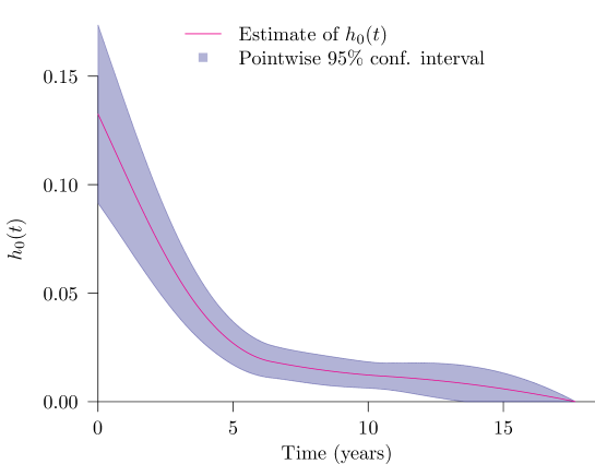
Figure 2: Plots of baseline hazard estimate and their 95% CI.

The hazard ratio estimates are exhibited in Table 6. Compared with melanoma that were first diagnosed at the head&neck, melanoma at arm or trunk have significantly lower risk of recurrence. Initial melanoma thickness is another strong risk factor for melanoma recurrence. A 10-year increase of age corresponds to a significant (9% to 21%) risk increase of melanoma recurrence. Gender is marginally significant, with women having a lower risk of melanoma recurrence than men.

The estimates of the baseline hazard function, together with its 95% pointwise confidence interval, is displayed in Figure 2. This plot indicates that when the covariates are all set to their baseline values, the risk of melanoma recurrence strongly and monotonically decreases during the first 5 years. Afterwards, during the next decade, the risk continue to regularly decrease to a level close to 0.

8 Conclusion

This paper develops a new approach for fitting a semi-parametric proportional hazard model where survival time observations include left, interval and right censoring times as well as event times. Since the baseline hazard is non-parametric and subject to a nonnegativity constraint we approximate this function using a finite number of nonnegative basis functions and we constrain the coefficients of the basis functions to be nonnegative. An efficient Newton-MI algorithm is developed. Asymptotic results establish that, under certain regularity conditions, when the number of knots goes to infinity (at a rate slower than the sample size goes to infinity) and the smoothing parameter goes to zero, both regression coefficients and baseline hazard MPL estimates are consistent almost surely. More practically useful asymptotic normality is developed and its standard errors are found to be accurate by the simulation study. We find the MPL estimates are capable of producing more satisfactory results than their competitors on both the regression coefficients and baseline hazard estimates. In particular, they produce regression coefficients with comparable (or smaller) biases and smaller standard errors. The 95% confidence intervals from the MPL estimates usually achieve better coverage probabilities (i.e. closer to 95%) than the competitors.

Appendices

Appendix A Components of score vector and Hessian matrix

Let $x_{ij}$ be element $j$ of vector $\mathbf{x}_{i}$. The first derivatives of $\Phi$ with respect to $\boldsymbol{\beta}$ and $\boldsymbol{\theta}$ are, for $j=1,\ldots,p$ and $u=1,\ldots,m$,

$$\frac{\partial\Phi(\boldsymbol{\beta},\boldsymbol{\theta})}{\partial\beta_{j}}= \sum_{i=1}^{n}x_{ij}\left(\delta_{i}-\delta_{i}H_{i}(t_{i})-\delta_{i}^{R}H_{i}(t_{i})+\delta_{i}^{L}\frac{S_{i}(t_{i})H_{i}(t_{i})}{1-S_{i}(t_{i})}\right.$$

$$\left.-\delta_{i}^{I}\frac{S_{i}(t_{i}^{L})H_{i}(t_{i}^{L})-S_{i}(t_{i}^{R})H_{i}(t_{i}^{R})}{S_{i}(t_{i}^{L})-S_{i}(t_{i}^{R})}\right),$$

$$\frac{\partial\Phi(\boldsymbol{\beta},\boldsymbol{\theta})}{\partial\theta_{u}}= \sum_{i=1}^{n}\left(\delta_{i}\frac{\psi_{u}(t_{i})}{h_{0}(t_{i})}-\delta_{i}\Psi_{u}(t_{i})e^{\mathbf{x}_{i}\boldsymbol{\beta}}-\delta_{i}^{R}\Psi_{u}(t_{i})e^{\mathbf{x}_{i}\boldsymbol{\beta}}+\delta_{i}^{L}\frac{S_{i}(t_{i})\Psi_{u}(t_{i})}{1-S_{i}(t_{i})}e^{\mathbf{x}_{i}\boldsymbol{\beta}}\right.$$

$$\left.-\delta_{i}^{I}\frac{S_{i}(t_{i}^{L})\Psi_{u}(t_{i}^{L})-S_{i}(t_{i}^{R})\Psi_{u}(t_{i}^{R})}{S_{i}(t_{i}^{L})-S_{i}(t_{i}^{R})}e^{\mathbf{x}_{i}\boldsymbol{\beta}}\right)-\lambda\frac{\partial J(\boldsymbol{\theta})}{\partial\theta_{u}},$$

where $\Psi_{u}(t)=\int_{0}^{T}\psi_{u}(\xi)d\xi$, the cumulative of basis function $\psi_{u}(t)$. Elements of the Hessian matrix are:

$$\frac{\partial^{2}\Phi(\boldsymbol{\beta},\boldsymbol{\theta})}{\partial\beta_{j}\partial\beta_{t}} =-\sum_{i=1}^{n}x_{ij}x_{it}\left(\delta_{i}H(t_{i})+\delta_{i}^{R}H(t_{i})+\delta_{i}^{L}\frac{S_{i}(t_{i})H_{i}(t_{i})(H_{i}(t_{i})+S_{i}(t_{i})-1)}{(1-S_{i}(t_{i}))^{2}}\right.$$

$$~{}+\left.\delta_{i}^{I}\frac{S_{i}(t_{i}^{L})S_{i}(t_{i}^{R})(-H_{i}(t_{i}^{L})+H_{i}(t_{i}^{R}))^{2}}{(S_{i}(t_{i}^{L})-S_{i}(t_{i}^{R}))^{2}}+\delta_{i}^{I}\frac{-S_{i}(t_{i}^{R})H_{i}(t_{i}^{R})+S_{i}(t_{i}^{L})H_{i}(t_{i}^{L})}{S_{i}(t_{i}^{L})-S_{i}(t_{i}^{R})}\right)$$

$$\frac{\partial^{2}\Phi(\boldsymbol{\beta},\boldsymbol{\theta})}{\partial\beta_{j}\partial\theta_{u}} =-\sum_{i=1}^{n}x_{ij}e^{\mathbf{x}_{i}\boldsymbol{\beta}}\left(\delta_{i}\Psi_{u}(t_{i})+\delta_{i}^{R}\Psi_{u}(t_{i})+\delta_{i}^{L}\frac{S_{i}(t_{i})}{1-S_{i}(t_{i})}\left[\frac{H_{i}(t_{i})}{1-S_{i}(t_{i})}-1\right]\right.$$

$$~{}+\delta_{i}^{I}\frac{S_{i}(t_{i}^{L})S_{i}(t_{i}^{R})(-H_{i}(t_{i}^{L})+H_{i}(t_{i}^{R}))(-\Psi_{u}(t_{i}^{L})+\Psi_{u}(t_{i}^{R}))}{(S_{i}(t_{i}^{L})-S_{i}(t_{i}^{R}))^{2}}$$

$$~{}+\left.\delta_{i}^{I}\frac{S_{i}(t_{i}^{L})\Psi_{u}(t_{i}^{L})-S_{i}(t_{i}^{R})\Psi_{u}(t_{i}^{R})}{S_{i}(t_{i}^{L})-S_{i}(t_{i}^{R})}\right)$$

$$\frac{\partial^{2}\Phi(\boldsymbol{\beta},\boldsymbol{\theta})}{\partial\theta_{u}\partial\theta_{v}} =-\sum_{i=1}^{n}\left(\delta_{i}\frac{\psi_{u}(t_{i})\psi_{v}(t_{i})}{h_{0}^{2}(t_{i})}+e^{2\mathbf{x}_{i}\boldsymbol{\beta}}\left[\delta_{i}^{L}\frac{S_{i}(t_{i})}{(1-S_{i}(t_{i}))^{2}}\Psi_{u}(t_{i})\Psi_{v}(t_{i})\right.\right.$$

$$~{}+\left.\left.\delta_{i}^{I}\frac{S_{i}(t_{i}^{L})S_{i}(t_{i}^{R})}{(S_{i}(t_{i}^{L})-S_{i}(t_{i}^{R}))^{2}}(\Psi_{u}(t_{i}^{R})-\Psi_{u}(t_{i}^{L}))(\Psi_{v}(t_{i}^{R})-\Psi_{v}(t_{i}^{L}))\right]\right)$$

Appendix B Sketch proof of Theorem 1

Our approach below closely follows the proofs given in Xue et al. (2004), Zhang et al. (2010) and Huang (1996). Recall $\boldsymbol{\tau}=(\boldsymbol{\beta},h_{0}(t))\in B*A$ and $\boldsymbol{\tau}_{n}=(\boldsymbol{\beta},h_{n}(t))\in B*A_{n}\subset B*A$, where spaces $B$, $A$ and $A_{n}$ have already been defined in Section 4. $h_{n}(t)$ is an approximation to $h_{0}(t)$ using the basis functions. The MPL estimator is represented by $\widehat{\boldsymbol{\tau}}_{n}$. For $\boldsymbol{\tau}_{1},\boldsymbol{\tau}_{2}\in B*A$, define a distance measure

$$\rho(\boldsymbol{\tau}_{1},\boldsymbol{\tau}_{2})=\{\|\boldsymbol{\tau}_{1}-\boldsymbol{\tau}_{2}\|^{2}\}^{1/2}=\left\{\|\boldsymbol{\beta}_{1}-\boldsymbol{\beta}_{2}\|_{2}^{2}+\sup_{t\in[a,b]}|h_{01}(t)-h_{02}(t)|^{2}\right\}^{1/2},$$

and we denote this measure by $L_{2}*L_{\infty}$.

The proofs below require the concept of covering number of a space; its definition can be found in, for example, Pollard (1984). Briefly, this is the number of spherical balls of a given size required to cover a given space. For a space $A$ with measure $\kappa(A)$, we denote the covering number associated with spheral radius $\varepsilon$ by $N(\varepsilon,A,\kappa(A))$.

Results 1 and 2 of Theorem 1 can be demonstrated if we are able to show that $\rho(\boldsymbol{\tau}_{0},\widehat{\boldsymbol{\tau}}_{n})\to 0$ (a.s.), where $\boldsymbol{\tau}_{0}=(\boldsymbol{\beta}_{0},h_{00}(t))$. Since the smoothing parameter $\mu_{n}\to 0$ when $n\to\infty$ and the penalty function is bounded, we can concentrated on the log-likelihood function only. The required result can be obtained through the following results.

1. Let $q(\boldsymbol{W};\boldsymbol{\tau})$ denote the Fréchet derivative of the density functional $f(\boldsymbol{W};\boldsymbol{\tau})$ with respect to $\boldsymbol{\tau}$. Let $\boldsymbol{\xi}$ be a point in between $\widehat{\boldsymbol{\tau}}_{n}$ and $\boldsymbol{\tau}_{0}$. Since $\boldsymbol{\xi}$ is not the maximum, the functional $q(\boldsymbol{W};\boldsymbol{\xi})$ is non-zero. Also, both $q(\boldsymbol{W};\boldsymbol{\xi})$ and $f(\boldsymbol{W};\boldsymbol{\xi})$ are bounded. According to the definition of $Pl(\boldsymbol{\tau})$ in Section 4 and the fact $\boldsymbol{\tau}_{0}$ maximizes $E_{0}l(\boldsymbol{\tau},\boldsymbol{W})$, we have

   $$|Pl(\widehat{\boldsymbol{\tau}}_{n};\boldsymbol{W})-Pl(\boldsymbol{\tau}_{0};\boldsymbol{W})|=E_{0}(l(\boldsymbol{\tau}_{0};\boldsymbol{W})-l(\widehat{\boldsymbol{\tau}}_{n};\boldsymbol{W}))$$

   $$\geq\|f^{\frac{1}{2}}(\boldsymbol{\tau}_{0};\boldsymbol{W})-f^{\frac{1}{2}}(\widehat{\boldsymbol{\tau}}_{n};\boldsymbol{W})\|_{2}^{2}=\left\|\frac{q(\boldsymbol{\xi};\boldsymbol{W})}{2f^{\frac{1}{2}}(\boldsymbol{\xi};\boldsymbol{W})}(\boldsymbol{\tau}_{0}-\widehat{\boldsymbol{\tau}}_{n})\right\|_{2}^{2}$$

   $$\geq C_{4}\|\boldsymbol{\tau}_{0}-\widehat{\boldsymbol{\tau}}_{n}\|_{2}^{2},$$ (15)

   where the first inequality is established since the Kullback-Leibler distance is not less than the Hellinger distance (Wong & Shen 1995), the second equality comes from the mean value theorem and $C_{4}$ is the lower bound of $|q(\boldsymbol{\xi};\boldsymbol{W})/2f^{\frac{1}{2}}(\boldsymbol{\xi};\boldsymbol{W})|$.

2. It then suffices to show $Pl(\widehat{\boldsymbol{\tau}}_{n})-Pl(\boldsymbol{\tau}_{0})\to 0$ almost surely. However, since

   $$|Pl(\widehat{\boldsymbol{\tau}}_{n})-Pl(\boldsymbol{\tau}_{0})|\leq|Pl(\widehat{\boldsymbol{\tau}}_{n})-P_{n}l(\widehat{\boldsymbol{\tau}}_{n})|+|P_{n}l(\widehat{\boldsymbol{\tau}}_{n})-Pl(\boldsymbol{\tau}_{0})|,$$

   we then wish to show that each term on the right hand side converges to 0 almost surely. For the first term, we just need to implement the result from part (3) below, but the second term demands further analyses. Define $\boldsymbol{\tau}_{0n}=(\boldsymbol{\beta}_{0},h_{0n}(t))\in B*A_{n}$, where $h_{0n}(t)$ is selected to satisfy $\rho(\boldsymbol{\tau}_{0n},\boldsymbol{\tau}_{0})\to 0$ (when $n\to\infty$), which is guaranteed by Assumption 4. Since $\boldsymbol{\tau}_{0}$ maximizes $Pl(\boldsymbol{\tau})$ for $\boldsymbol{\tau}\in B*A$ and $\widehat{\boldsymbol{\tau}}_{n}$ maximizes $P_{n}l(\boldsymbol{\tau})$ for $\boldsymbol{\tau}\in B*A_{n}$, we have

   $$P_{n}l(\boldsymbol{\tau}_{0n})-Pl(\boldsymbol{\tau}_{0n})+Pl(\boldsymbol{\tau}_{0n})-Pl(\boldsymbol{\tau}_{0})\leq P_{n}l(\widehat{\boldsymbol{\tau}}_{n})-Pl(\boldsymbol{\tau}_{0})\leq P_{n}l(\widehat{\boldsymbol{\tau}}_{n})-Pl(\widehat{\boldsymbol{\tau}}_{n}).$$

   From part (3) below we have both $P_{n}l(\widehat{\boldsymbol{\tau}}_{n})-Pl(\widehat{\boldsymbol{\tau}}_{n})$ and $P_{n}l(\boldsymbol{\tau}_{0n})-Pl(\boldsymbol{\tau}_{0n})$ converge to 0 almost surely. $Pl(\boldsymbol{\tau}_{0n})-Pl(\boldsymbol{\tau}_{0})$ converges to 0 can be established from $\rho(\boldsymbol{\tau}_{0n},\boldsymbol{\tau}_{0})\to 0$ and the fact that $l(\cdot)$ is continuous and bounded.

3. It suffices to demonstrate $\sup_{\boldsymbol{\tau}_{n}\in B*A_{n}}|P_{n}l(\boldsymbol{\tau}_{n})-Pl(\boldsymbol{\tau}_{n})|\to 0$ almost surely. This can be achieved through the following steps:

   1. Firstly, we show that $N(\varepsilon,A_{n},L_{\infty})\leq(6C_{5}C_{6}/\varepsilon)^{m}$ where constants $C_{5}$ and $C_{6}$ will be specified below. This is because for any $h_{n1},h_{n2}\in A_{n}$ (hence each $h_{nj}(t)=\sum_{u}\theta_{un}^{j}\psi_{u}(t)$), $\max_{t}|h_{n1}(t)-h_{n2}(t)|\leq C_{5}\max_{u}|\theta_{un}^{1}-\theta_{un}^{2}|\leq C_{5}\|\boldsymbol{\theta}^{1}-\boldsymbol{\theta}^{2}\|_{2}$, where $C_{5}$ is the upper bound of $\sum_{u}\psi_{u}(t)$ and $\boldsymbol{\theta}^{j}$ is an $m$-vector with elements $\theta_{un}^{j}$. Thus, $N(\varepsilon,A_{n},L_{\infty})\leq N(\varepsilon/C_{5},\{0\leq\theta_{un}\leq C_{6},1\leq u\leq m\},L_{2})\leq(6C_{5}C_{6}/\varepsilon)^{m}$, and the last inequality comes from Lemma 4.1 of Pollard (1984).

   2. Secondly we wish to demonstrate that $N(\varepsilon,{\cal L}_{n},L_{\infty})\leq K/\varepsilon^{p+m}$, where the constant $K$ will be explicated below and ${\cal L}_{n}=\{l(\boldsymbol{\tau}_{n}),\boldsymbol{\tau}_{n}\in B*A_{n}\}$. In fact, $N(\varepsilon,{\cal L}_{n},L_{\infty})\leq N(\varepsilon/2,B,L_{2})\cdot N(\varepsilon/2,A_{n},L_{\infty})\leq(12C_{1}/\varepsilon)^{p}(12C_{5}C_{6}/\varepsilon)^{m}=K/\varepsilon^{p+m}$, where $C_{1}$ is the upper bound of $\{|\beta_{j}|,\forall j\}$ and $K=12^{p+m}C_{1}^{p}(C_{5}C_{6})^{m}$.

   3. Select $\alpha_{n}=n^{-1/2+\phi_{1}}\sqrt{\log n}$ where $\phi_{1}\in(\phi_{0}/2,1/2)$ with $\phi_{0}<1$, and define $\varepsilon_{n}=\varepsilon\alpha_{n}$. Following Theorem 1 of Xue et al. (2004) we can show that $\text{var}[P_{n}l(\boldsymbol{\tau}_{n})]/(8\varepsilon_{n}^{2})\to 0$ when $n\to\infty$ for any $\boldsymbol{\tau}_{n}\in B*A_{n}$.

   4. Finally, from the result II.31 of Pollard (1984), we have

      $$P[\sum_{B*A_{n}}|P_{n}l(\boldsymbol{\tau}_{n})-P_{n}l(\boldsymbol{\tau})|>8\varepsilon_{n}]\leq 8N(\varepsilon_{n},{\cal L}_{n},L_{\infty})e^{-\frac{1}{128}n\varepsilon_{n}^{2}}$$

      $$\leq 8Ke^{-\left(\frac{1}{128}\varepsilon^{2}+\frac{p+m}{2}\frac{\log(\varepsilon^{2}n^{-1+2\phi_{1}}\log n)}{n^{2\phi_{1}}\log n}\right)n^{2\phi_{1}}\log n},$$

      which converges to zero as the second term in bracket of the exponential function goes to zero when $n\to\infty$. Therefore, by the Borel-Cantelli lemma, we have $\sup_{B*A_{n}}|P_{n}l(\boldsymbol{\tau}_{n})-Pl(\boldsymbol{\tau}_{n})|\to 0$ almost surely.

Appendix C Sketch proof of Theorem 2

Let $\overline{l}(\boldsymbol{\eta})=E_{\boldsymbol{\eta}_{0}}[n^{-1}l(\boldsymbol{\eta})]$. It follows from the strong law of large numbers that $n^{-1}l(\boldsymbol{\eta})\rightarrow\overline{l}(\boldsymbol{\eta})$ almost surely and uniformly for $\boldsymbol{\eta}\in\Omega$. This result, together with $\mu_{n}\to 0$ as $n\to\infty$ and $\boldsymbol{\eta}_{0}$ being the unique maximum of $\overline{l}(\boldsymbol{\eta})$ due to Assumption B2, implies that $\widehat{\boldsymbol{\eta}}\rightarrow\boldsymbol{\eta}_{0}$ almost surely by applying, for example, Corollary 1 of Honore & Powell (1994).

Next we prove the asymptotic normality result. From the KKT necessary conditions (6) and (7) we have that the constrained MPL estimate $\widehat{\boldsymbol{\eta}}$ satisfies

$$\mathbf{U}^{T}\frac{\partial\Phi(\widehat{\boldsymbol{\eta}})}{\partial\boldsymbol{\eta}}=0,$$ (16)

where $\mathbf{U}$ is defined in equation (10) of section 4.3. According to the Taylor expansion

$$\frac{\partial\Phi(\widehat{\boldsymbol{\eta}})}{\partial\boldsymbol{\eta}}=\frac{\partial\Phi(\boldsymbol{\eta}_{0})}{\partial\boldsymbol{\eta}}+\frac{\partial^{2}\Phi(\widetilde{\boldsymbol{\eta}})}{\partial\boldsymbol{\eta}\partial\boldsymbol{\eta}^{\text{T}}}(\widehat{\boldsymbol{\eta}}-\boldsymbol{\eta}_{0}),$$ (17)

where $\widetilde{\boldsymbol{\eta}}$ is a vector between $\widehat{\boldsymbol{\eta}}$ and $\boldsymbol{\eta}_{0}$. Therefore

$$0=\mathbf{U}^{T}\frac{\partial\Phi(\boldsymbol{\eta}_{0})}{\partial\boldsymbol{\eta}}+\mathbf{U}^{T}\frac{\partial^{2}\Phi(\widetilde{\boldsymbol{\eta}})}{\partial\boldsymbol{\eta}\partial\boldsymbol{\eta}^{\text{T}}}(\widehat{\boldsymbol{\eta}}-\boldsymbol{\eta}_{0}).$$ (18)

Next, let $\widehat{\boldsymbol{\chi}}$ be $\widehat{\boldsymbol{\eta}}$ after deleting the active constraints and $\boldsymbol{\chi}_{0}$ be similarly defined corresponding to $\boldsymbol{\eta}_{0}$, then

$$\widehat{\boldsymbol{\eta}}-\boldsymbol{\eta}_{0}=\mathbf{U}(\widehat{\boldsymbol{\chi}}-\boldsymbol{\chi}_{0}).$$ (19)

Substituting (19) into (18), solving for $\widehat{\boldsymbol{\chi}}-\boldsymbol{\chi}_{0}$ and then using (19) to convert the result back to $\widehat{\boldsymbol{\eta}}-\boldsymbol{\eta}_{0}$ again, we eventually have

$$\sqrt{n}(\widehat{\boldsymbol{\eta}}-\boldsymbol{\eta}_{0})=-\mathbf{U}\left(\mathbf{U}^{T}\frac{1}{n}\frac{\partial^{2}\Phi(\widetilde{\boldsymbol{\eta}})}{\partial\boldsymbol{\eta}\partial\boldsymbol{\eta}^{T}}\mathbf{U}\right)^{-1}\mathbf{U}^{T}\left(\frac{1}{\sqrt{n}}\frac{\partial l(\boldsymbol{\eta}_{0})}{\partial\boldsymbol{\eta}}+o(1)\right).$$ (20)

In (20), $-n^{-1}\partial^{2}\Phi(\boldsymbol{\eta})/\partial\boldsymbol{\eta}\partial\boldsymbol{\eta}^{T}$ converges to $F(\boldsymbol{\eta})$ (a.s.) by the law of large numbers. Also note that $\widetilde{\boldsymbol{\eta}}\to\boldsymbol{\eta}_{0}$ almost surely. Then after applying the central limit theorem to $n^{-1/2}\partial l(\boldsymbol{\eta}_{0})/\partial\boldsymbol{\eta}$ we have the required asymptotic normality result.

Appendix D M-spline and Gaussian basis functions

If the baseline hazard is approximated by Gaussian basis functions, $\psi_{u}(t)$ is a truncated Gaussian distribution with location parameter $\alpha_{u}$ (which are knots), scale parameter $\sigma_{u}$ and range $[t_{(1)},t_{(n)}]$. This leads to the following expressions of $\psi_{u}(t)$ and its cumulative function $\Psi_{u}(t)$:

$$\psi_{u}(t) =\frac{1}{\sigma_{u}\delta_{u}}\phi\left(\frac{t-\alpha_{u}}{\sigma_{u}}\right),~{}$$

$$\Psi_{u}(t) =\int\limits_{t_{(1)}}^{t}\psi_{u}(v)dv=\frac{1}{\Delta_{u}}\left[\Phi\left(\frac{t-\alpha_{u}}{\sigma_{u}}\right)-\Phi\left(\frac{t_{(1)}-\alpha_{u}}{\sigma_{u}}\right)\right],$$

where $t_{(1)}\leq t\leq t_{(n)}$, $\phi(\cdot)$ and $\Phi(\cdot)$ respectively are the density and cumulative density functions of the standard Gaussian distribution, $\Delta_{u}=\Phi((t_{(n)}-\alpha_{u})/\sigma_{u})-\Phi((t_{(1)}-\alpha_{u})/\sigma_{u})$ and $\alpha_{u}\in\mathbb{R}$ and $\sigma_{u}>0$. If the baseline hazard is approximated by means of M$-$spline basis functions of order $o$ (Ramsay 1988), we get the following expressions of $\psi^{o}_{u}(t)$ and $\Psi^{o}_{u}(t)$:

$$\psi^{o}_{u}(t) =\begin{cases}\frac{\delta(\alpha^{\star}_{u}\leq t<\alpha^{\star}_{u+1})}{\alpha^{\star}_{u+1}-\alpha^{\star}_{u}}&\text{if }o=1,\\ \frac{o}{o-1}\frac{\delta(\alpha^{\star}_{u}\leq t<\alpha^{\star}_{u+o})}{\alpha^{\star}_{u+o}-\alpha^{\star}_{u}}\left[\left(t-\alpha^{\star}_{u}\right)\psi^{o-1}_{u}(t)+\left(\alpha^{\star}_{u+o}-t\right)\psi^{o-1}_{u+1}(t)\right]&\text{otherwise},\end{cases}$$

$$\Psi^{o}_{u}(t) =\delta(\alpha^{\star}_{u}>t)\left[\sum\limits_{v=u+1}^{\text{min}(u+o,m+1)}\frac{\alpha^{\star\star}_{v+o+1}-\alpha^{\star\star}_{v}}{o+1}\psi^{o+1}_{v}(t)\right]^{\delta(\alpha^{\star}_{u}<t<\alpha^{\star}_{u+o})},$$

where $t_{(1)}\leq t\leq t_{(n)}$, $\alpha_{u}$ is the $u$th element of knots vector $\boldsymbol{\alpha}$ whose length is $n_{\alpha}$ ($\alpha_{u}\in\mathbb{R}$ and $\alpha_{u}<\alpha_{u+1}$), $m=n_{\alpha}+o-2$, $\boldsymbol{\alpha}^{\star}=\left[\min(\boldsymbol{\alpha})\mathbf{1}^{T}_{o-1},\boldsymbol{\alpha}^{T},\max(\boldsymbol{\alpha})\mathbf{1}^{T}_{o-1}\right]^{T}$, and $\boldsymbol{\alpha}^{\star\star}=\left[\min(\boldsymbol{\alpha})\mathbf{1}^{T}_{o},\boldsymbol{\alpha}^{T},\max(\boldsymbol{\alpha})\mathbf{1}^{T}_{o}\right]^{T}$, where $\mathbf{1}_{o}$ denotes a vector of 1 of length $o$. Note that $\Psi^{o}_{u}(t)$, the cumulative function of $\psi^{o}_{u}(t)$, is referred to as an I$-$spline. M$-$spline basis functions have the following properties: $\int_{-\infty}^{\alpha^{\star}_{u}}\psi^{o}_{u}(v)dv=0$, $\int_{\alpha^{\star}_{u}}^{\alpha^{\star}_{u+o}}\psi^{o}_{u}(v)dv=1$ and $\int_{\alpha^{\star}_{u+o}}^{\alpha^{\star}_{\infty}}\psi^{o}_{u}(v)dv=0$.

Appendix E Simulation results related to baseline hazard functions

In this section we present simulation results regarding to $h_{0}(t)$ from the three simulations. Specifically, tables 7 – 9 report biases, mean asymptotic and Monte Carlo standard errors and 95% coverage probabilities, all at 25%, 50% and 75% quantile points of $h_{0}(t)$. Figure 1 displays the true $h_{0}(t)$, the average MPL $h_{0}(t)$ estimates and pointwise 95% confidence intervals.

Figure 3: Mean baseline hazard estimates and their pointwise 95% confidence intervals.

		$\pi^{E}=0\%$		$\pi^{E}=10\%$		$\pi^{E}=25\%$		$\pi^{E}=50\%$
		$n=200$	$n=500$	$n=200$	$n=500$	$n=200$	$n=500$	$n=200$	$n=500$
Biases
$h_{0}(t_{1})$	Breslow	4.982	4.918	4.608	4.517	4.258	4.294	3.877	3.661
	CM	0.182	0.197	-0.300	-0.449	-0.430	-0.436	-0.296	-0.304
	LPS	-0.096	-0.062	-0.101	-0.048	-0.073	-0.042	-0.053	-0.027
	EM-I	-0.032	-0.100	-0.027	-0.064	-0.021	-0.021	-0.016	-0.002
	MPL-M	0.014	0.014	0.019	0.009	0.021	0.009	0.026	0.011
	MPL-G	0.007	0.005	0.017	0.016	0.022	0.027	0.025	0.027
$h_{0}(t_{2})$	Breslow	1.180	1.113	1.403	1.250	1.535	1.586	1.490	1.798
	CM	0.189	0.064	-0.162	-0.192	-0.160	-0.197	-0.147	-0.194
	LPS	0.006	0.014	-0.013	0.020	0.013	0.006	0.018	0.012
	EM-I	0.011	0.131	0.021	0.081	0.018	0.027	0.020	0.008
	MPL-M	0.028	0.012	0.029	0.010	0.026	0.009	0.025	0.011
	MPL-G	-0.009	0.015	0.006	0.027	0.006	0.023	0.011	0.024
$h_{0}(t_{3})$	Breslow	4.256	2.740	4.037	2.627	2.394	2.220	1.900	2.186
	CM	0.085	-0.092	0.037	-0.084	0.020	-0.142	-0.045	-0.097
	LPS	0.052	0.000	0.019	0.005	0.018	-0.001	0.005	0.000
	EM-I	-0.016	-0.064	-0.038	-0.051	-0.039	-0.022	-0.028	-0.003
	MPL-M	0.020	0.007	0.025	0.014	0.025	0.013	0.025	0.013
	MPL-G	-0.080	-0.037	-0.065	-0.017	-0.043	0.007	-0.012	0.018
Mean asymptotic (Monte Carlo) standard errors
$h_{0}(t_{1})$	Breslow	-	-	-	-	-	-	-	-
		(4.521)	(3.583)	(3.889)	(3.471)	(4.539)	(3.622)	(4.724)	(3.556)
	CM	-	-	-	-	-	-	-	-
		(0.666)	(0.812)	(0.367)	(0.430)	(0.321)	(0.286)	(0.317)	(0.359)
	LPS	0.106	0.075	0.101	0.071	0.098	0.067	0.094	0.064
		(0.112)	(0.081)	(0.108)	(0.076)	(0.101)	(0.071)	(0.100)	(0.064)
	EM-I	0.150	0.136	0.130	0.102	0.121	0.089	0.108	0.078
		(0.122)	(0.082)	(0.119)	(0.081)	(0.111)	(0.078)	(0.104)	(0.070)
	MPL-M	0.093	0.061	0.089	0.056	0.083	0.0512	0.076	0.047
		(0.101)	(0.064)	(0.094)	(0.058)	(0.084)	(0.050)	(0.077)	(0.046)
	MPL-G	0.113	0.073	0.111	0.072	0.107	0.070	0.101	0.066
		(0.115)	(0.071)	(0.113)	(0.073)	(0.107)	(0.068)	(0.102)	(0.064)
$h_{0}(t_{2})$	Breslow	-	-	-	-	-	-	-	-
		(3.717)	(2.525)	(4.719)	(2.667)	(3.538)	(3.027)	(2.856)	(6.237)
	CM	-	-	-	-	-	-	-	-
		(1.384)	(1.379)	(0.790)	(0.776)	(0.667)	(0.590)	(0.741)	(0.552)
	LPS	0.173	0.120	0.163	0.113	0.157	0.106	0.149	0.099
		(0.171)	(0.120)	(0.170)	(0.109)	(0.160)	(0.101)	(0.152)	(0.092)
	EM-I	0.265	0.265	0.218	0.189	0.195	0.150	0.167	0.122
		(0.183)	(0.168)	(0.176)	(0.152)	(0.165)	(0.133)	(0.153)	(0.118)
	MPL-M	0.149	0.095	0.141	0.088	0.131	0.082	0.119	0.074
		(0.152)	(0.095)	(0.148)	(0.088)	(0.131)	(0.079)	(0.119)	(0.073)
	MPL-G	0.157	0.103	0.156	0.103	0.151	0.100	0.143	0.094
		(0.165)	(0.103)	(0.163)	(0.104)	(0.151)	(0.096)	(0.142)	(0.093)
$h_{0}(t_{3})$	Breslow	-	-	-	-	-	-	-	-
		(68.918)	(22.245)	(58.760)	(19.951)	(6.620)	(6.557)	(3.883)	(5.947)
	CM	-	-	-	-	-	-	-	-
		(1.477)	(1.207)	(1.219)	(0.979)	(1.124)	(0.909)	(1.049)	(1.074)
	LPS	0.281	0.186	0.251	0.169	0.231	0.156	0.209	0.142
		(0.290)	(0.186)	(0.250)	(0.169)	(0.227)	(0.156)	(0.211)	(0.134)
	EM-I	0.547	0.292	0.345	0.211	0.272	0.184	0.220	0.160
		(0.318)	(0.210)	(0.278)	(0.190)	(0.237)	(0.171)	(0.206)	(0.153)
	MPL-M	0.227	0.144	0.213	0.134	0.198	0.123	0.178	0.111
		(0.232)	(0.146)	(0.219)	(0.135)	(0.196)	(0.121)	(0.177)	(0.110)
	MPL-G	0.227	0.151	0.215	0.147	0.206	0.142	0.195	0.132
		(0.240)	(0.155)	(0.231)	(0.153)	(0.212)	(0.143)	(0.200)	(0.136)
95% coverage probabilities
$h_{0}(t_{1})$	LPS	0.916	0.916	0.938	0.934	0.939	0.938	0.939	0.958
	EM-I	0.949	0.980	0.933	0.959	0.933	0.965	0.930	0.959
	MPL-M	0.923	0.931	0.927	0.937	0.932	0.957	0.948	0.947
	MPL-G	0.924	0.947	0.922	0.944	0.936	0.956	0.945	0.951
$h_{0}(t_{2})$	LPS	0.938	0.940	0.950	0.958	0.939	0.962	0.955	0.960
	EM-I	0.977	0.998	0.963	0.989	0.958	0.964	0.959	0.954
	MPL-M	0.936	0.940	0.940	0.944	0.942	0.957	0.950	0.956
	MPL-G	0.918	0.946	0.933	0.947	0.937	0.947	0.938	0.945
$h_{0}(t_{3})$	LPS	0.942	0.972	0.954	0.962	0.941	0.950	0.954	0.958
	EM-I	0.990	0.980	0.953	0.945	0.930	0.956	0.934	0.951
	MPL-M	0.933	0.942	0.934	0.935	0.946	0.957	0.949	0.956
	MPL-G	0.861	0.899	0.864	0.925	0.901	0.944	0.920	0.942
Integrated discrepancy between $\widehat{h}_{0}(t)$ and $h_{0}(t)$ defined between 0 and the 90th percentile of $T$
	Breslow	7.203	4.331	3.161	2.752	2.808	2.662	2.668	2.594
	CM	0.914	0.724	0.778	0.651	0.697	0.603	0.663	0.600
	EM-I	0.341	0.204	0.271	0.171	0.231	0.146	0.192	0.125
	MPL-M	0.192	0.125	0.182	0.111	0.161	0.097	0.145	0.089
	MPL-G	0.227	0.143	0.224	0.144	0.204	0.130	0.177	0.112

Table 7: Simulation 1 results for $h_{0}(t)$ for the 25th ($t_{1}$), 50th ($t_{2}$), and 75th ($t_{3}$) percentiles of T. Some results are missing for the convex minorant estimator as no inference was not developed for this estimator, for the penalized spline estimator as the information was missing in the article of (Cai & Betensky 2003, Section 6), and for the Breslow estimator as we did not compute estimate the variance for this estimator.

		$\pi^{E}=0\%$			$\pi^{E}=25\%$			$\pi^{E}=50\%$
		$n=100$	$n=500$	$n=2000$	$n=100$	$n=500$	$n=2000$	$n=100$	$n=500$	$n=2000$
Biases
$h_{0}(t_{1})$	Breslow	-0.367	-0.288	-0.276	-0.239	-0.080	-0.124	-0.183	-0.161	-0.038
	CM	-0.019	-0.155	-0.371	-0.420	-0.464	-0.438	-0.290	-0.259	-0.284
	EM-I	0.015	0.049	0.035	0.012	0.014	0.016	-0.007	-0.007	0.009
	MPL-M	0.133	0.042	0.020	0.126	0.029	0.012	0.107	0.016	0.009
	MPL-G	0.114	0.041	0.009	0.078	0.024	0.012	0.048	0.012	0.005
$h_{0}(t_{2})$	Breslow	-0.082	-0.177	-0.315	-0.048	-0.130	-0.186	-0.035	-0.069	-0.142
	CM	0.300	-0.224	-0.371	-0.429	-0.315	-0.250	-0.226	-0.224	-0.258
	EM-I	0.300	0.036	0.021	0.201	0.018	0.012	0.119	0.009	0.007
	MPL-M	0.060	0.032	0.026	0.051	0.034	0.016	0.039	0.025	0.010
	MPL-G	0.071	0.064	0.033	0.071	0.036	0.011	0.044	0.018	0.009
$h_{0}(t_{3})$	Breslow	0.225	0.024	0.025	0.082	-0.009	0.039	0.039	0.052	-0.076
	CM	0.416	-0.411	-0.601	-0.424	-0.594	-0.618	-0.384	-0.504	-0.550
	EM-I	0.481	0.055	-0.019	0.183	0.062	0.017	0.117	0.046	0.010
	MPL-M	-0.072	-0.044	-0.014	-0.060	-0.003	0.008	-0.054	0.003	0.008
	MPL-G	0.003	-0.035	0.009	0.042	0.015	0.012	0.029	0.014	0.006
Mean asymptotic (Monte Carlo) standard errors
$h_{0}(t_{1})$	Breslow	-	-	-	-	-	-	-	-	-
		(0.816)	(1.873)	(1.380)	(1.296)	(4.470)	(1.913)	(1.094)	(1.367)	(2.672)
	CM	-	-	-	-	-	-	-	-	-
		(1.437)	(1.326)	(0.921)	(0.680)	(0.551)	(0.552)	(1.050)	(0.850)	(0.683)
	EM-I	0.789	0.429	0.193	0.588	0.255	0.139	0.495	0.215	0.124
		(0.629)	(0.366)	(0.162)	(0.544)	(0.246)	(0.132)	(0.468)	(0.196)	(0.119)
	MPL-M	0.547	0.224	0.115	0.478	0.196	0.101	0.425	0.176	0.092
		(0.592)	(0.233)	(0.121)	(0.488)	(0.206)	(0.102)	(0.428)	(0.178)	(0.093)
	MPL-G	0.567	0.236	0.123	0.491	0.213	0.116	0.437	0.194	0.104
		(0.619)	(0.253)	(0.127)	(0.517)	(0.227)	(0.116)	(0.448)	(0.203)	(0.103)
$h_{0}(t_{2})$	Breslow	-	-	-	-	-	-	-	-	-
		(3.137)	(3.580)	(1.781)	(3.157)	(3.680)	(2.762)	(3.369)	(3.747)	(2.779)
	CM	-	-	-	-	-	-	-	-	-
		(4.134)	(2.766)	(2.980)	(1.618)	(1.827)	(2.316)	(2.361)	(1.677)	(2.493)
	EM-I	2.196	0.988	0.540	1.4831	0.596	0.320	1.169	0.486	0.254
		(2.005)	(0.805)	(0.425)	(1.504)	(0.592)	(0.318)	(1.106)	(0.439)	(0.253)
	MPL-M	1.061	0.454	0.231	0.914	0.397	0.201	0.812	0.354	0.180
		(1.292)	(0.482)	(0.233)	(0.971)	(0.412)	(0.199)	(0.816)	(0.358)	(0.180)
	MPL-G	1.109	0.481	0.247	0.982	0.424	0.222	0.866	0.379	0.200
		(1.254)	(0.507)	(0.252)	(1.057)	(0.439)	(0.225)	(0.896)	(0.380)	(0.200)
$h_{0}(t_{3})$	Breslow	-	-	-	-	-	-	-	-	-
		(7.646)	(13.574)	(7.210)	(6.311)	(12.815)	(7.612)	(5.466)	(11.052)	(5.933)
	CM	-	-	-	-	-	-	-	-	-
		(9.568)	(3.735)	(3.773)	(3.341)	(2.569)	(2.154)	(3.438)	(2.215)	(2.276)
	EM-I	6.659	1.596	1.195	3.189	1.143	0.553	2.373	0.981	0.447
		(6.979)	(1.525)	(0.719)	(3.190)	(1.119)	(0.539)	(2.366)	(0.969)	(0.434)
	MPL-M	1.828	0.854	0.465	1.603	0.769	0.404	1.447	0.691	0.359
		(2.412)	(0.946)	(0.482)	(1.848)	(0.803)	(0.392)	(1.586)	(0.711)	(0.353)
	MPL-G	2.090	0.892	0.494	1.901	0.829	0.445	1.684	0.751	0.398
		(2.379)	(0.997)	(0.518)	(2.117)	(0.868)	(0.434)	(1.803)	(0.779)	(0.390)
95% coverage probabilities
$h_{0}(t_{1})$	EM-I	0.904	0.969	0.981	0.883	0.954	0.968	0.894	0.940	0.957
	MPL-M	0.922	0.945	0.941	0.926	0.935	0.951	0.932	0.931	0.950
	MPL-G	0.908	0.928	0.948	0.906	0.928	0.952	0.925	0.929	0.946
$h_{0}(t_{2})$	EM-I	0.960	0.975	0.985	0.917	0.937	0.947	0.912	0.951	0.945
	MPL-M	0.881	0.933	0.957	0.908	0.936	0.952	0.915	0.948	0.945
	MPL G	0.884	0.946	0.948	0.917	0.939	0.943	0.916	0.940	0.947
$h_{0}(t_{3})$	EM-I	0.970	0.959	0.998	0.921	0.953	0.965	0.899	0.951	0.954
	MPL-M	0.735	0.868	0.925	0.793	0.919	0.949	0.821	0.935	0.953
	MPL-G	0.829	0.855	0.930	0.872	0.924	0.951	0.875	0.939	0.949
Integrated discrepancy between $\widehat{h}_{0}(t)$ and $h_{0}(t)$ defined between 0 and the 90th percentile of $T$
	Breslow	17.450	6.233	4.159	3.823	2.673	2.215	3.230	2.659	2.105
	CM	5.173	2.416	2.564	2.626	2.457	2.328	2.558	2.276	2.072
	EM-I	5.227	1.150	0.593	2.274	0.786	0.392	1.684	0.655	0.333
	MPL-M	1.615	0.727	0.389	1.352	0.591	0.292	1.176	0.518	0.265
	MPL-G	1.581	0.808	0.443	1.398	0.641	0.323	1.232	0.565	0.294

Table 8: Simulation 2 results for $h_{0}(t)$ for the 25th ($t_{1}$), 50th ($t_{2}$), and 75th ($t_{3}$) percentiles of T. Some results are missing for the convex minorant estimator as no inference was not developed for this estimator, and for the Breslow estimator as we did not estimate the variance for this estimator.

		$\pi^{E}=0\%$			$\pi^{E}=25\%$			$\pi^{E}=50\%$
		$n=100$	$n=500$	$n=2000$	$n=100$	$n=500$	$n=2000$	$n=100$	$n=500$	$n=2000$
Biases
$h_{0}(t_{1})$	Breslow	-0.360	-0.446	-0.464	-0.190	-0.185	-0.269	1.735	0.244	-0.002
	CM	0.194	0.170	0.114	-0.201	-0.167	-0.239	0.086	0.128	0.059
	EM-I	0.024	0.303	0.334	-0.068	0.027	0.070	-0.122	-0.037	0.061
	MPL-M	-0.004	-0.020	0.010	-0.018	-0.014	0.013	-0.029	-0.025	0.014
	MPL-G	0.050	0.032	0.025	0.017	0.020	0.013	0.017	0.016	0.011
$h_{0}(t_{2})$	Breslow	-0.378	-0.354	-0.383	-0.225	-0.183	-0.270	-0.160	-0.078	-0.081
	CM	0.591	0.150	0.120	-0.222	-0.111	-0.154	-0.012	0.074	-0.004
	EM-I	0.127	0.295	0.403	0.081	0.079	0.004	0.034	0.016	-0.003
	MPL-M	-0.123	-0.100	-0.050	-0.110	-0.067	-0.021	-0.107	-0.049	-0.010
	MPL-G	-0.084	-0.058	-0.027	-0.061	-0.030	-0.012	-0.037	-0.018	-0.004
$h_{0}(t_{3})$	Breslow	-0.247	-0.287	-0.140	-0.160	-0.202	-0.114	-0.112	-0.200	-0.128
	CM	1.024	0.149	0.011	-0.342	-0.597	-0.624	-0.399	-0.439	-0.423
	EM-I	0.173	0.086	0.081	0.141	0.011	0.090	0.079	0.018	0.025
	MPL-M	-0.139	-0.115	-0.078	-0.112	-0.085	-0.043	-0.105	-0.065	-0.027
	MPL-G	-0.166	-0.104	-0.055	-0.104	-0.062	-0.031	-0.077	-0.041	-0.017
Mean asymptotic (Monte Carlo) standard errors
$h_{0}(t_{1})$	Breslow	-	-	-	-	-	-	-	-	-
		(1.746)	(0.787)	(0.780)	(1.417)	(1.182)	(0.956)	(61.436)	(9.629)	(3.133)
	CM	-	-	-	-	-	-	-	-	-
		(1.409)	(1.817)	(2.620)	(1.019)	(0.825)	(0.817)	(1.478)	(1.391)	(1.259)
	EM-I	0.630	0.415	0.257	0.432	0.276	0.129	0.375	0.195	0.122
		(0.407)	(0.309)	(0.154)	(0.388)	(0.241)	(0.117)	(0.349)	(0.182)	(0.114)
	MPL-M	0.397	0.190	0.110	0.349	0.170	0.096	0.314	0.154	0.087
		(0.424)	(0.201)	(0.115)	(0.373)	(0.185)	(0.098)	(0.329)	(0.156)	(0.090)
	MPL-G	0.451	0.211	0.113	0.398	0.184	0.098	0.370	0.170	0.088
		(0.447)	(0.216)	(0.117)	(0.418)	(0.195)	(0.102)	(0.375)	(0.170)	(0.091)
$h_{0}(t_{2})$	Breslow	-	-	-	-	-	-	-	-	-
		(2.492)	(2.276)	(1.929)	(2.663)	(2.738)	(1.948)	(2.543)	(2.825)	(3.222)
	CM	-	-	-	-	-	-	-	-	-
		(5.265)	(4.801)	(3.890)	(1.664)	(1.709)	(1.655)	(1.856)	(2.125)	(1.704)
	EM-I	0.970	0.619	0.515	0.818	0.493	0.231	0.751	0.377	0.192
		(0.981)	(0.460)	(0.241)	(0.811)	(0.395)	(0.213)	(0.714)	(0.318)	(0.188)
	MPL-M	0.632	0.293	0.169	0.558	0.268	0.151	0.500	0.249	0.138
		(0.686)	(0.319)	(0.180)	(0.603)	(0.301)	(0.156)	(0.538)	(0.263)	(0.146)
	MPL-G	0.676	0.316	0.173	0.616	0.286	0.154	0.577	0.266	0.141
		(0.708)	(0.329)	(0.178)	(0.661)	(0.306)	(0.157)	(0.603)	(0.267)	(0.147)
$h_{0}(t_{3})$	Breslow	-	-	-	-	-	-	-	-	-
		(2.764)	(2.655)	(7.332)	(4.076)	(3.246)	(6.000)	(4.199)	(3.127)	(5.241)
	CM	-	-	-	-	-	-	-	-	-
		(10.753)	(5.271)	(5.261)	(2.779)	(1.310)	(0.966)	(1.755)	(1.450)	(1.769)
	EM-I	1.577	0.814	0.463	1.282	0.584	0.351	1.134	0.497	0.296
		(1.656)	(0.571)	(0.256)	(1.318)	(0.477)	(0.312)	(1.012)	(0.452)	(0.274)
	MPL-M	0.938	0.422	0.227	0.832	0.376	0.205	0.741	0.345	0.188
		(1.064)	(0.459)	(0.238)	(0.949)	(0.420)	(0.216)	(0.839)	(0.373)	(0.201)
	MPL-G	0.912	0.429	0.233	0.856	0.390	0.210	0.790	0.362	0.192
		(0.999)	(0.455)	(0.235)	(0.968)	(0.416)	(0.215)	(0.847)	(0.380)	(0.201)
Empirical 95% coverage probabilities
$h_{0}(t_{1})$	EM-I	0.947	0.925	0.765	0.874	0.940	0.953	0.839	0.911	0.949
	MPL-M	0.859	0.917	0.942	0.881	0.909	0.947	0.879	0.934	0.938
	MPL-G	0.899	0.947	0.940	0.903	0.935	0.938	0.905	0.950	0.942
$h_{0}(t_{2})$	EM-I	0.910	0.821	0.691	0.881	0.972	0.962	0.895	0.961	0.953
	MPL-M	0.786	0.810	0.859	0.802	0.849	0.920	0.807	0.890	0.934
	MPL-G	0.828	0.896	0.922	0.851	0.898	0.928	0.871	0.939	0.938
$h_{0}(t_{3})$	EM-I	0.948	0.949	0.975	0.921	0.953	0.934	0.935	0.944	0.968
	MPL-M	0.757	0.775	0.772	0.793	0.801	0.877	0.784	0.845	0.893
	MPL-G	0.731	0.801	0.850	0.805	0.863	0.910	0.823	0.882	0.914
Integrated discrepancy between $\widehat{h}_{0}(t)$ and $h_{0}(t)$ defined between 0 and the 90th percentile of $T$
	Breslow	0.810	0.739	0.573	0.789	0.704	0.521	0.775	0.688	0.495
	CM	1.277	0.691	0.589	0.705	0.588	0.573	0.623	0.529	0.522
	EM-I	0.383	0.223	0.207	0.327	0.153	0.094	0.288	0.136	0.077
	MPL-M	0.326	0.161	0.089	0.287	0.139	0.070	0.259	0.121	0.063
	MPL-G	0.317	0.153	0.079	0.285	0.130	0.068	0.255	0.116	0.060

Table 9: Simulation 3 results for $h_{0}(t)$ for the 25th ($t_{1}$), 50th ($t_{2}$), and 75th ($t_{3}$) percentiles of T. Some results are missing for the convex minorant estimator as no inference was not developed for this estimator, and for the Breslow estimator as we did not estimate the variance for this estimator.

References

- (1)
- Armijo (1966) Armijo, L. (1966), ‘Minimization of functions having lipschitz-continuous first partial derivatives’, Pacific Journal of Mathematics 16, 1–3.
- Cai & Betensky (2003) Cai, T. & Betensky, R. A. (2003), ‘Hazard regression for interval-censored data with penalized spline’, Biometrics 59, 570–579.
- Chan & Ma (2012) Chan, R. H. & Ma, J. (2012), ‘A multiplicative iterative algorithm for box-constrained penalized likelihood image restoration’, IEEE Trans. Image Processing 21, 3168–3181.
- Chen et al. (2012) Chen, D.-G., Sun, J. & Peace, K. E. (2012), Interval-Censored Time-to-Event Data: Methods and Applications, Chapman and Hall/CRC.
- Crowder (1984) Crowder, M. (1984), ‘On constrained maximum likelihood estimation with non-i.i.d. observations’, Ann. Inst. Stat. Math. 36, 239–249.
- DeBoor & Daniel (1974) DeBoor, C. & Daniel, J. W. (1974), ‘Splines with nonnegative B-spline coefficients’, Mathematics of Computation 126, 565–568.
- Finkelstein (1986) Finkelstein, D. M. (1986), ‘A proportional hazard model for interval-censored failure time data’, Biometrics 42, 845–854.
- Green & Silverman (1994) Green, P. J. & Silverman, B. W. (1994), Nonparametric Regression and Generalized Linear Models - A roughness penealty approach, Chapman and Hall, London.
- Grenander (1981) Grenander, U. (1981), Abstract Inference, J. Wiley, New York.
- Groeneboom & Wellner (1992) Groeneboom, P. & Wellner, J. A. (1992), Information bounds and nonparametric maximum likelihood estimation, Birkhauser, Basel.
- Honore & Powell (1994) Honore, B. E. & Powell, J. L. (1994), ‘Pairwise difference estimators of censored and truncated regression models’, Journal of Econometrics 64, 241–278.
- Huang (1996) Huang, J. (1996), ‘Efficient estimation for the proportional hazard model with interval censoring’, The Annals of Statistics 24, 540 – 568.
- Joly et al. (1998) Joly, P., Commenges, D. & Letenneur, L. (1998), ‘A penalized likelihood approach for arbitrarily censored and truncated data: application to age-specific incidence of dementia’, Biometrics 54, 185–194.
- Kim (2003) Kim, J. S. (2003), ‘Maximum likelihood estimation for the proportional hazard model with partly interval-censored data’, J. Roy. Statist. Soc. B 65, 489–502.
- Luenberger (1984) Luenberger, D. (1984), Linear and Nonlinear Programming (2nd edition), J. Wiley.
- Ma et al. (2014) Ma, J., Heritier, S. & Lô, S. (2014), ‘On the maximum penalized likelihood approach for proportional hazard models with right censored survival data’, Computational Statistics and Data Analysis 74, 142–156.
- Moore et al. (2008) Moore, T. J., Sadler, B. M. & Kozick, R. J. (2008), ‘Maximum-likelihood estimation, the Cramér -Rao bound, and the method of scoring with parameter constraints’, IEEE Trans. Sig. Proc. 56, 895–908.
- Morton et al. (2014) Morton, D., Thompson, J., Cochran, A., Mozzillo, N., Nieweg, O., Roses, D., Hoekstra, H., Karakousis, C., Puleo, C., Coventry, B., Kashani-Sabet, M., Smithers, B., Paul, E., Kraybill, W., McKinnon, J., Wang, H.-J., Elashoff, R., Faries, M. & for the MSLT Group (2014), ‘Final trial report of sentinel-node biopsy versus nodal observation in melanoma’, The New England Journal of Medicine 307, 599–609.
- Pan (1999) Pan, W. (1999), ‘Extending the iterative convex minorant algorithm to the Cox model for interval-censored data’, Journal of Computational and Graphical Statistics 8, 109–120.
- Pollard (1984) Pollard, D. (1984), Convergence of stochastic processes, Springer Verlag, New York.
- Ramsay (1988) Ramsay, J. O. (1988), ‘Monotone regression splines in action’, Statistical Science 3, 425–441.
- Sun (2006) Sun, J. (2006), The statistical analysis of interval-censored failure time data, Springer.
- Wang et al. (2016) Wang, L., McMahan, C., Hudgens, M. & Qureshi, Z. (2016), ‘A flexible, computationally efficient method for fitting the proportional hazards model to interval-censored data’, Biometrics 72, 222–231.
- Wong & Severini (1991) Wong, W. H. & Severini, T. A. (1991), ‘On maximum likelihood estimation in infinite dimensional parameter spaces’, Ann. Statist. 19, 603–632.
- Wong & Shen (1995) Wong, W. H. & Shen, X. (1995), ‘Probability inequalities for likelihood ratios and convergene rates of sieve MLEs’, Ann. Statist. 23, 339–362.
- Xue et al. (2004) Xue, H., Lam, K. F. & Li, G. (2004), ‘Sieve maximum likelihood estimator for semiparametric regression models with current status data’, J. Amer. Statist. Assoc. 99, 346–356.
- Zhang et al. (2010) Zhang, Y., Hua, L. & Huang, J. (2010), ‘A spline-based semiparametric maximum likelihood esimation method for the Cox model with interval-censored data’, Scand. J. Statist. 37, 338–354.