Electronic friction in interacting systems

Abstract

We consider effects of strong light-matter interaction on electronic friction in molecular junctions within generic model of single molecule nano cavity junction. Results of the Hubbard NEGF simulations are compared with mean-field NEGF and generalized Head-Gordon and Tully approaches. Mean-field NEGF is shown to fail qualitatively at strong intra-system interactions, while accuracy of the generalized Head-Gordon and Tully results is restricted to situations of well separated intra-molecular excitations, when bath induced coherences are negligible. Numerical results show effects of bias and cavity mode pumping on electronic friction. We demonstrate non-monotonic behavior of the friction on the bias and intensity of the pumping field and indicate possibility of engineering friction control in single molecule junctions.

I Introduction

Dynamics of open quantum systems is an active area of reasearch due to its fundamental complexity and promise of technological applications. In single molecules and single molecule junctions, many studies forcus on dynamics caused by interactions between electronic and vibrational degrees of freedom in the molecule. In particular, the interactions are central to spectroscopy Bennett et al. (2016); Petit and Subotnik (2015, 2014a, 2014b), bias-induced Jiang et al. (2016); Ouyang et al. (2015) and photo-chemistry Lei et al. (2016), electron  Wang et al. (2015) and energy Imada et al. (2017, 2016); Lee et al. (2016); Krüger et al. (2015) transfer, coherent control Tiwari and Henriksen (2016), radiative Miwa et al. (2019) and non-radiative Long et al. (2016) electronic relaxation, and stability of junctions Nitzan and Galperin (2018); Gelbwaser-Klimovsky et al. (2018); Foti and Vázquez (2018); Simine and Segal (2012); Lü et al. (2011). Understanding mechanisms of the interactions and developing theoretical description is crucial for engineering optoelectronic Ohmura et al. (2016); Nelson et al. (2014) and optomechanical Nikiforov et al. (2016) molecular devices.

Current-induced nuclear forces is an important part of such considerations directly related to study of dynamics in open nonequilibrium molecular systems under assumption of time scale separation between electronic and nuclear degrees of freedom (the Born-Oppenheimer approximation). The time scale separation allows formulation of the stochastic Langevin equation for classical molecular nuclei driven by quantum nonequilibrium electronic subsystem. Electronic degrees of freedom induce renormalization of the adiabatic nuclear potential and lead to appearance of electronic friction and stochastic forces. The latter two are related by the fluctuation-dissipation theorem. Roughly, theoretical derivations can be separated to exact considerations within path-integral Brandbyge et al. (1995); Lü et al. (2012, 2015) or scattering Thomas et al. (2012); Bode et al. (2011, 2012) approaches and to more qualitative formulations employing quantum-classical Liouville equation Shenvi and Tully (2012); Falk et al. (2014); Dou et al. (2015); Dou and Subotnik (2016); Dou et al. (2017); Dou and Subotnik (2017). Some formulations of electronic friction even rely on Golden rule type derivations Askerka et al. (2016); Maurer et al. (2016). In terms of accounting for interactions within the electronic subsystem, exact considerations were mostly restricted to mean-field level of treatment. Recently, more general exact considerations started to appear capable of taking into account intra-molecular interactions within perturbative diagrammatic expansion in the interactions strengths Hopjan et al. (2018); Kantorovich (2018). However, strong intra-system interactions are beyond capabilities of these approaches.

Recently, we formulated general derivation of the current-induced nuclear forces applicable in nonequilibrium molecular systems with arbitrary intra-system interactions Chen et al. (2019). The derivation is valid for any strength and form of interactions in electronic subsystem and/or between electronic and nuclear degrees of freedom. We showed that electronic friction can be expressed in terms of retarded projections of single-particle nonequilibirum Hubbbard Green function. The Hubbard NEGF - recently introduced by us many-body flavor of nonequilibrium Green function method Chen et al. (2017) - appears to be reasonably accurate in a wide range of parameters Miwa et al. (2017). We note in passing that formulations of electronic friction in standard NEGF results in two-particle Green function - an object much harder to handle than single-particle result of the Hubbard NEGF. The Hubbard NEGF uses many-body molecular states as a basis. Thus, all intra-system interactions are taken into account exactly. In this respect it is similar to the quantum master equation (QME) formulations. However, contrary to standard QME (such as, e.g., Lindblad/Redfield QME), the Hubbard NEGF is a diagrammatic expansion in the system-bath(s) coupling(s), which means that under a particular order in expansion one sums all diagrams of this order. Thus, the methodology overcomes usual restrictions ($k_{B}T\gg\Gamma$, where $k_{B}T$ is thermal energy and $\Gamma$ electron escape rate) of the QME schemes and is capable of accounting for non-Markov character of system-bath dynamics.

Here, we apply the Hubbard NEGF to study effects of strong intra-system interactions on electronic friction. In particular, we consider single-molecule cavity junction and discuss effects of strong light-matter (plamson-molecular exciton) interaction on electronic friction. We note that strong light-matter interaction in single molecule junctions was recently demonstrated experimentally in scanning tunneling microscope-induced plasmonic nanocavities Kongsuwan et al. (2018); Chikkaraddy et al. (2016). While so far only optical response of the junction has been studied, similar measurements in current-carrying molecular junctions will probably become a reality in the nearest future.

Structure of the paper is the following. In Section II we introduce a model of molecular junction and give brief introduction to the Hubbard NEGF and to way of simulating electronic friction. Numerical results and discussion are presented in Section III. Section IV summarizes our findings and outlines goals for future research.

II Model and method

We consider junction which consists of a molecule in nanocavity coupled to metallic contacts and to external radiation field. Molecule is modeled as two-level system, $\varepsilon_{m}$ ($m=1,2$) with electron hopping $t$ between the levels and with coupling to two vibrational modes, $Q_{1}$ and $Q_{2}$. The modes will be treated classically - we will be interested in electronic friction (dissipative part of electronic force) acting on the nuclear motion. Nanocavity is represented by single cavity mode modeled as harmonic oscillator of frequency $\omega_{c}$. The mode is coupled to molecular exciton, modeled as transition between the two levels, and to external radiation field. Two contacts, $L$ and $R$, are modeled as free electron reservoirs, each at its own equilibrium. Radiation field $rad$ serves as energy drain for the cavity mode, it also can be used to pump the mode. Hamiltonian of the model is

$$\begin{split}\hat{H}&=\hat{H}_{0}+\hat{H}_{1}+\hat{H}_{vib}\\ \hat{H}_{0}&=\hat{H}_{sys}+\hat{H}_{bath}\\ \hat{H}_{1}&=\hat{V}_{ML}+\hat{V}_{MR}+\hat{V}_{c,rad}\end{split}$$ (1)

where

$$\begin{split}\hat{H}_{sys}&=\hat{H}_{M}+\hat{H}_{c}+\hat{V}_{M,c}\\ \hat{H}_{bath}&=\hat{H}_{L}+\hat{H}_{R}+\hat{H}_{rad}\end{split}$$ (2)

Here $\hat{H}_{sys}$ and $\hat{H}_{bath}$ are the system and baths Hamiltonians. $\hat{H}_{M}$, $\hat{H}_{c}$, $\hat{H}_{L}$, $\hat{H}_{R}$ and $\hat{H}_{rad}$ are respectively Hamiltonians of the molecule, cavity mode, left and right contacts, and radiation field. Operators $\hat{V}$ introduce coupling between the subsystems. $\hat{H}_{vib}$ is Hamiltonian representing vibrational degrees of freedom. Explicit expressions are

$$\hat{H}_{M} =\sum_{m=1,2}\varepsilon_{m}\hat{d}_{m}^{\dagger}\hat{d}_{m}-t\left(\hat{d}_{1}^{\dagger}\hat{d}_{2}+\hat{d}_{2}^{\dagger}\hat{d}_{1}\right)$$ (3)

$$\hat{H}_{c} =\omega_{c}\hat{a}_{c}^{\dagger}\hat{a}_{c}$$ (4)

$$\hat{H}_{K} =\sum_{k\in K}\varepsilon_{k}\hat{c}_{k}^{\dagger}\hat{c}_{k}\quad(K=L,R)$$ (5)

$$\hat{H}_{rad} =\sum_{\alpha}\omega_{\alpha}\hat{a}_{\alpha}^{\dagger}\hat{a}_{\alpha}$$ (6)

$$\hat{V}_{M,c} =U_{c}\left(\hat{a}_{c}+\hat{a}_{c}^{\dagger}\right)\left(\hat{d}_{1}^{\dagger}\hat{d}_{2}+\hat{d}_{2}^{\dagger}\hat{d}_{1}\right)$$ (7)

$$\hat{V}_{MK} =\sum_{k\in K}\left(V_{mk}\hat{d}_{m}^{\dagger}\hat{c}_{k}+H.c.\right)\quad(m=1(2)\mbox{ for }K=L(R))$$ (8)

$$\hat{V}_{c,rad} =\sum_{\alpha}\left(U_{\alpha}\hat{a}_{c}^{\dagger}\hat{a}_{\alpha}+H.c.\right)$$ (9)

$$\hat{H}_{vib} =\frac{1}{2}\sum_{v=1,2}\left(\hat{P}_{v}^{2}+\hat{Q}_{v}^{2}\right)+M^{(1)}\left(\hat{d}_{1}^{\dagger}\hat{d}_{2}+\hat{d}_{2}^{\dagger}\hat{d}_{1}\right)\hat{Q}_{1}+M^{(2)}\left(\hat{d}_{1}^{\dagger}\hat{d}_{1}-\hat{d}_{2}^{\dagger}\hat{d}_{2}\right)\hat{Q}_{2}$$ (10)

Here $\hat{d}_{m}^{\dagger}$ ($\hat{d}_{m}$) and $\hat{c}_{k}^{\dagger}$ ($\hat{c}_{k}$) create (annihilate) electron on molecular level $m$ and state $k$ of the contacts, respectively. $\hat{a}_{c}^{\dagger}$ ($\hat{a}_{c}$) and $\hat{a}_{\alpha}^{\dagger}$ ($\hat{a}_{\alpha}$) excites (destroys) quanta in the cavity mode and mode $\alpha$ of the radiation field. Note that Hamiltonian $\hat{H}_{vib}$ representing vibrational degrees of freedom and their coupling to electronic degrees of freedom is only used to derive expression for the electronic friction (see Ref. Chen et al. (2019) for details) and does not participate in further numerical analysis. Indeed, electron induced nuclear forces (including friction) can be introduced only for classical nuclei Thus, vibrational Hamiltonian $\hat{H}_{vib}$ is only necessary as a starting point of a derivation reducing full quantum description of nuclei to their classical behavior. After the derivation is finished, expression for the forces (including friction) depend on electronic degrees of freedom only and vibrational Hamiltonian does not participate in further analysis. Still, we show the $\hat{H}_{vib}$ because it defines electron-nuclear coupling $M^{(1,2)}$ used in the considerations below. Note that in realistic simulation for strictly adiabatic limit of nuclear dynamics electronic structure depends on static nuclear configuration. This means that parameters of electronic Hamiltonian (such as level positions $\varepsilon_{m}$, electron hopping $t$, coupling to contacts $V_{mk}$, etc.) depend on nuclear positions. In the analysis below we utilize set of fixed parameters, which may be considered as values corresponding to one nuclear frame.

We note that in (2) $\hat{V}_{M,c}$ was put into the system Hamiltonian $H_{sys}$ to allow consideration of strong light-matter interaction. Clearly, quasiparticle representation is not the most convenient way to treat $\hat{V}_{M,c}$. Instead, we utilize the Born-Oppenheimer type many-body states as a basis for our consideration

$$\lvert S\rangle=\lvert e\rangle\,\lvert p\rangle$$ (11)

Here $\lvert e\rangle$ represents one of four possible electronic states: empty state $\lvert 0,0\rangle$, electron in level $1$ $\lvert 1,0\rangle$, electron in level $2$ $\lvert 0,1\rangle$, and two electrons in the molecule $\lvert 1,1\rangle$. $\lvert p\rangle$ are states of the harmonic oscillator representing the cavity mode. Using spectral decompositions of the second quantized operators in the many-body states

$$\hat{d}_{m}^{\dagger} =\sum_{S_{1},S_{2}}\lvert S_{2}\rangle\langle S_{2}\rvert\hat{d}_{m}^{\dagger}\lvert S_{1}\rangle\langle S_{1}\rvert\equiv\sum_{S_{1},S_{2}}\delta_{p_{2},p_{1}}\xi^{m}_{e_{2},e_{1}}\hat{X}_{S_{1}S_{2}}^{\dagger}$$ (12)

$$\hat{a}_{c}^{\dagger} =\sum_{S_{1},S_{2}}\lvert S_{2}\rangle\langle S_{2}\rvert\hat{a}_{c}^{\dagger}\lvert S_{1}\rangle\langle S_{1}\rvert\equiv\sum_{S_{1},S_{2}}\delta_{e_{2},e_{1}}\delta_{p_{2},p_{1}+1}\sqrt{p_{2}}\,\hat{X}_{S_{1}S_{2}}^{\dagger}$$ (13)

one can represent the model in many-body basis of the zero-order Hamiltonian with baths ($L$, $R$, and $rad$) still represented in standard second quantization (see Appendix A for explicit form of the Hamiltonian).

After transformation to many-body eigenstates of the Hamiltonian $\hat{H}_{sys}$,

$$\hat{H}_{sys}=\sum_{S}E_{S}\hat{X}_{SS},$$ (14)

we introduce single-particle Hubbard Green’s function

$$G_{(S_{1}S_{2})(S_{3}S_{4})}(\tau,\tau^{\prime})=-i\langle T_{c}\,\hat{X}_{S_{1}S_{2}}(\tau)\,\hat{X}_{S_{3}S_{4}}^{\dagger}(\tau^{\prime})\rangle$$ (15)

Here $T_{c}$ is the Keldysh contour ordering operator, $\tau$ and $\tau^{\prime}$ are the contour variables, and

$$\hat{X}_{S_{1}S_{2}}\equiv\lvert S_{1}\rangle\langle S_{2}\rvert$$ (16)

is the Hubbard operator. Following Ref. Chen et al. (2017) one has to solve the modified Dyson equation with self-energies due to coupling to the contacts and to the radiation field evaluated within nonequilibrium diagrammatic technique for the Hubbard Green functions. The solution is self-consistent because the self-energies both define Green functions (via the modified Dyson equation) and depend on them (via self-energies expressions). In the consideration below we utilize second order diagrammatic expansion in the system-baths couplings. Short details about the self-consistent procedure and explicit forms of the self-energies are given in Appendix B.

Once Green function (15) is known, following our derivation in Ref. Chen et al. (2019) we calculate electronic friction for the model (1) as

$$\gamma_{ab}(E)=\sum_{S_{1},S_{2},S_{3},S_{4}}M^{(a)}_{S1S_{2}}\,G^{r}_{(S_{1}S_{2})(S_{3}S_{4})}(E)\,M^{(b)}_{S_{4}S_{3}}$$ (17)

where $M^{(a)}_{S_{1}S_{2}}$ and $M^{(b)}_{S_{4}S_{3}}$ ($a,b=1,2$) are the electron-vibration interactions $M^{(1)}$ and $M^{(2)}$ introduced in (10) represented in the many-body eigenbasis of the Hamiltonian $\hat{H}_{0}$. $G^{r}_{(S_{1}S_{2})(S_{3}S_{4})(E)}$ is the Fourier transform of retarded projection of the Hubbard Green’s function (15). We note in passing that the friction tensor (17) has two nuclear indices because nuclear quantum deviations from classical trajectory in derivation of Ref. Chen et al. (2019) are taken into account up to second order in cumulant expansion. Higher order expansion would result in more nuclear indices (one for every additional order). We also note that while in the model (for simplicity and in order to demonstrate accuracy of our Hubbard NEGF method in non-interacting case, where exact solution is known) we consider linear electron-nuclei coupling, the derivation in Ref. Chen et al. (2019) and expression for friction are more general.

III Results and discussion

Unless stated otherwise parameters of the simulations are the following. Simulations are performed at room temperature $T=300$ K and molecular levels are set as $\varepsilon_{1}=-\varepsilon_{2}=0.1$ eV with electron hopping parameter $t=0.1$ eV. Strength of coupling between electronic and vibrational degrees of freedom is $M^{(1)}=M^{(2)}=0.01$ eV and molecular exciton coupling to cavity mode (the strong light-matter interaction parameters) is $U_{c}=0.5$ eV. Electron escape rates to metallic contacts

$$\Gamma^{K}_{m_{1}m_{2}}(E)\equiv 2\pi\sum_{k\in K}V_{m_{1}k}V_{km_{2}}\delta(E-\varepsilon_{k})$$ (18)

are assumed to be energy independent (the wide band approximation), they are $\Gamma^{L(R)}_{m_{1}m_{2}}=\delta_{m_{1},m_{2}}\,\delta_{m_{1},1(2)}\,0.1$ eV. Frequency of the cavity mode is taken as $\omega_{c}=0.2$ eV and the mode energy dissipation rate

$$\gamma_{c}(\omega)\equiv 2\pi\sum_{\alpha}\lvert U_{\alpha}\rvert^{2}\delta(\omega-\omega_{\alpha})$$ (19)

(also assumed to be energy independent) is $0.01$ eV. Fermi energy is taken as an origin, $E_{F}=0$, and bias $V_{sd}$ is applied symmetrically, $\mu_{L}=E_{F}+\lvert e\rvert V_{sd}/2$ and $\mu_{R}=E_{F}-\lvert e\rvert V_{sd}/2$. Unless specified otherwise, we take $V_{sd}=1$ V. Radiation field is modeled as continuum of modes with modes around frequency of the laser, $\omega_{0}$ being populated as

$$N(\omega)=I_{0}\,\frac{\delta^{2}}{(\omega-\omega_{0})^{2}+\delta^{2}}$$ (20)

Here $\delta$ is the laser bandwidth and $I_{0}$ is its intensity. Below we take $\omega_{0}=0.2$ eV and $\delta=0.1$ eV. $I_{0}=1$ in the presence of pumping and $0$ otherwise. Simulations are performed on an adjustable grid. The self-consistent calculation is assumed to be converged when populations of many-body states at subsequent steps of the procedure differ no more than $0.01$.

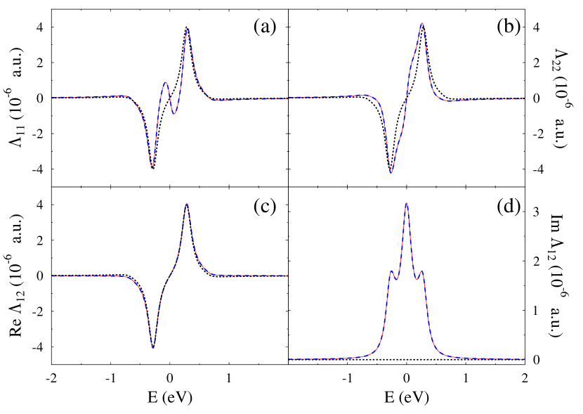
Figure 1: Friction tensor $\Lambda(E)$, Eq. (21), for non-interacting model, $U_{c}=0$. Shown are exact result (solid line, red), the Hubbard NEGF simulation (dashed line, blue), and results obtained using nonequilibrium generalization of the Head-Gordon and Tully electronic friction (dotted line, black). Parameters of the simulations are $T=300$ K, $\varepsilon_{1}=-\varepsilon_{2}=0.1$ eV, $t=0.1$ eV, $M^{(1)}=M^{(2)}=0.01$ eV, $\Gamma^{L(R)}_{m_{1}m_{2}}=\delta_{m_{1},m_{2}}\,\delta_{m_{1},1(2)}\,0.1$ eV, and $V_{sd}=1$ V.

We start from a non-interacting case, $U_{c}=0$, exact results for which were originally derived in Ref. Lü et al. (2012). To facilitate comparison with that work, we consider the $\Lambda_{ab}(E)$ function, which is related to the friction tensor (17) in time domain as

$$\gamma_{ab}(t)=2\pi i\,\theta(t)\,\Lambda_{ab}(t)$$ (21)

Figure 1 shows elements of the tensor simulated within the standard NEGF (exact result) and the Hubbard NEGF. We also show results calculated using generalized version of the celebrated Head-Gordon and Tully (HGT) expression for electronic friction. Note that the original HGT expression is derived from consideration of a time-dependent Schrödinger equation and states of electronic system are expressed in terms of ‘single determinantal wave functions. Note also that the original HGT friction kernel is of the second order in non-adiabatic transfer element. This means that the original consideration is performed for an isolated molecule (no baths at all), and that the consideration is restricted to non-interacting (mean-filed) electronic systems with weak electron-nuclei coupling. Our recent publication, Ref. Chen et al. (2019), generalizes the HGT expression to open nonequilibrium interacting (beyond mean field) systems with arbitrary (both in form and strength) electron-nuclei coupling (see Ref. Chen et al. (2019) for details). However, even this generalized version of the HGT expression misses bath-induced coherences which become important in quasi-degenerate situations when energy separation between many-body states of electronic system are smaller than characteristic energy scale of the system-bath interaction. Below we demonstrate failure of the expression comparing it to results of the Hubbard NEGF simulations. Fig. 1 is similar to Fig. 3 of Ref. Chen et al. (2019); but calculated for a different set of parameters. As previously, Hubbard NEGF is pretty accurate in reproducing exact results. For smaller $\Gamma$ considered here, the generalized Head-Gordon and Tully expression becomes quite accurate near molecular resonances ($\sqrt{(\varepsilon_{1}-\varepsilon_{2})^{2}+4t^{2}}$), while still missing coherence related contributions: $\Lambda_{11}(E)$ near $E=0$ and $\mbox{Im}\,\Lambda_{12}(E)$. We note in passing that at $E>0$ areas with $\Lambda<0$ correspond to usual friction (i.e. situation when electronic bath slows down nuclear motion), while areas with $\Lambda>0$ correspond to nuclear motion being speeded up by the electronic subsystem. Please note that such vibrational instability (negative friction caused by a population-inverted situation) was discussed in prior publications (see, e.g., Ref. Lü et al. (2012)).

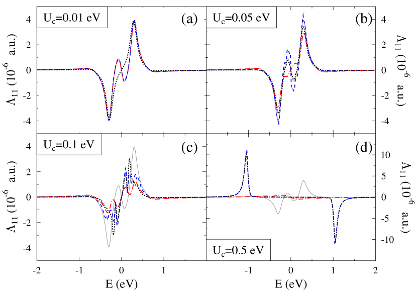
Figure 2: Friction tensor $\Lambda_{11}(E)$, Eq. (21), in the presence of molecular exciton-cavity mode coupling, $U_{c}$. Panels (a)-(d) show results for several values of the interaction. Each panel presents results of simulations within the mean-field NEGF (dash-dotted line, red), the Hubbard NEGF (dashed line, blue), and nonequilibrium generalization of the Head-Gordon and Tully electronic friction (dotted line, black). For comparison, solid gray line shows exact non-interacting, $U_{c}=0$, result. Cavity mode frequency is $\omega_{c}=0.2$ eV. Other parameters are as in Fig. 1.

Next we consider effect of molecular exciton-cavity mode coupling on electronic friction. Figure 2 shows results of simulations for the $\Lambda_{11}$ elements of the friction tensor, Eq. (21), for a set of interaction strengths. We compare the Hubbard NEGF with the generalized version of the Head-Gordon and Tully expression and to mean-field NEGF treatment of Ref. Lü et al. (2012) (details of the NEGF Green function simulations are given in Appendix C). We see that for extremely weak interaction (Fig. 2a) mean field and Hubbard NEGF yield the same result; with the interaction growing (Fig. 2b) the two approaches start to deviate from each other. For intermediate interaction strength (Fig. 2c) molecule-cavity mode coupling slightly reduces electronic friction. We attribute the effect to relatively lower values for the coupling $M^{(1)}$ for separate channels (transitions between different pairs of the many-body states) in the many-body eigenbasis. At strong coupling (Fig. 2d) the Hubbard NEGF shows enhanced electronic friction, while mean field NEGF predicts reduction in the friction. The reason for discrepancy is importance of intra-system correlations between electronic and cavity mode degrees of freedom. This is missed by the mean-field NEGF treatment. Note that inadequacy of mean-field predictions of electronic friction was also shown in Refs. Dou et al. (2017); Hopjan et al. (2018).

The generalized Head-Gordon and Tully result quite expectedly becomes accurate in the case of strong coupling between molecular exciton and cavity mode. Indeed, strong intra-system interaction is equivalent to relatively weak system-bath coupling (i.e. we are in regime where bath induced correlations between many-body eigenstates of the system become less important). Relative accuracy of the generalized Head-Gordon and Tully expression in the case of weak system-bath interaction was demonstrated in our previous study Chen et al. (2019) for a non-interacting model. As we showed in that study, nonequilibrium generalization of the Head-Gordon and Tully result comes from $S_{1}=S_{3}$ and $S_{2}=S_{4}$ subset of terms in the general expression (17). For relatively weak system-bath coupling one can further simplify the analysis by going to quasiparticle limit . Under these approximations, electronic friction (21) can be written as

$$\Lambda_{ab}(E)\approx\sum_{S_{1},S_{2}}M^{(a)}_{S_{1}S_{2}}M^{(b)}_{S_{2}S_{1}}\big{(}P_{S_{2}}-P_{S_{1}}\big{)}\,\delta\big{(}E-\left[E_{S_{2}}-E_{S_{1}}\right]\big{)}$$ (22)

Here $P_{S}$ is probability of the eigenstate $\lvert S\rangle$ to be populated and $E_{S}$ is its energy.

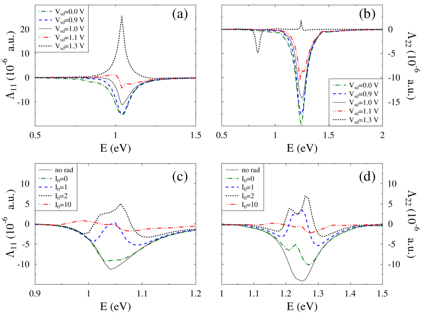
Figure 3: Control of electronic friction by external perturbations in the strong coupling regime $U_{c}=0.5$ eV. Shown are the Hubbard NEGF results for (a) $\Lambda_{11}(E)$ and (b) $\Lambda_{22}(E)$ for several biases $V_{sd}$ in the absence of radiation field; (c) $\Lambda_{11}(E)$ and $\Lambda_{22}(E)$ for several intensities $I_{0}$ of radiation field at $V_{sd}=1$ V. Pumping radiation field is taken at resonance with cavity mode, $\omega_{0}=0.2$ eV. Laser bandwidth is $\delta=0.1$ eV. Simulations presented in panels (a) and (b) are performed in the absence of pumping, $I_{0}=0$; bias in simulations presented in panels (c) and (d) is $V_{sd}=1$ V. Other parameters are as in Fig. 2.

Eq. (22) indicates that peaks in the friction correspond to electronic transitions within charging block and that sign and value of the friction are defined by probabilities of the corresponding many-body eigenstates. Thus, controlling the probabilities allows to engineer the friction: equal probabilities yield zero contribution of the transition to electronic friction, maximum contribution is for transition between empty and filled states. Such control can be achieved, e.g., by changing external bias or by pumping the cavity mode. Figures 3a and b show control of electronic friction for vibrational modes $1$ and $2$, respectively. Simulations are performed within the Hubbard NEGF for for strong light-matter coupling, $U_{c}=0.5$ eV. One sees that friction dependence on the bias is non-monotonic. That is, at higher biases and hence for higher currents, one can get smaller friction. For the considered parameters $V_{sd}=1.1$ V minimizes friction for the mode $1$ and $V_{sd}=1.3$ V friction is minimal for mode $2$. Similarly, control of electronic friction for the two vibrational modes by pumping cavity mode with external radiation field is shown in Figures 3c and d, respectively. Note that even in absence of pumping, $I_{0}=0$, friction for isolated cavity mode differs from the result for mode coupled to empty radiation field due to energy damping in the latter case. Also here friction behaves non-monotonically with intensity of the field, and for the parameters chosen minimum of electronic friction is achieved for $I_{0}=10$.

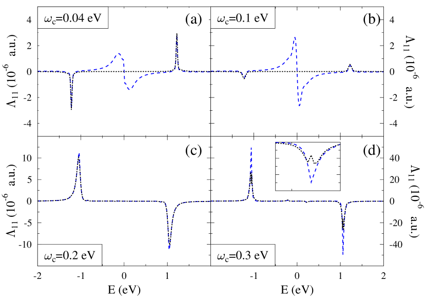
Figure 4: Friction tensor $\Lambda_{11}(E)$, Eq. (21), in the presence of molecular exciton-cavity mode coupling, $U_{c}=0.5$ eV. Panels (a)-(d) show results for several values of cavity mode frequency $\omega_{c}$. Each panel presents results of simulations within the Hubbard NEGF (dashed line, blue), and nonequilibrium generalization of the Head-Gordon and Tully electronic friction (dotted line, black). Inset in panel (d) shows the peak at $E\sim 1$ eV in more details. Simulations are performed at bias $V_{sd}=1$ V in the absence of pumping, $I_{0}=0$. Other parameters are as in Fig. 3.

Finally, we note that even at strong light-matter interaction, the generalized Head-Gordon and Tully expression is accurate only near resonance, $\omega_{c}\approx\varepsilon_{1}-\varepsilon_{2}$. In an off-resonant situation bath-induces coherence between close (relative to $\Gamma$) molecular resonances, are beyond the expression capabilities. Figure 4 shows electronic friction $\Lambda_{11}(E)$ at strong exciton-cavity mode coupling of $U_{c}=0.5$ eV for a set of cavity mode frequencies. One sees that the Hubbard NEGF coincides with the Head-Gordon and Tully result only at resonant $\omega_{c}$ (see Fig. 4c). Any shift out of the resonance condition, so that $\omega_{c}-\lvert\varepsilon_{1}-\varepsilon_{2}\rvert\geq\Gamma$, leads to discrepancy between the two results (see Figs. 4a, b, and d).

IV Conclusion

We discuss electronic friction in interacting systems. In particular, we consider a model of a junction consisting of single molecule in nano cavity with strong light-matter interaction. Such systems have been realized experimentally; however, so far measurements were restricted to unbiased junctions. Recently, we derived general expression for electronic friction in interacting systems Chen et al. (2019). We showed that the friction can be conveniently expressed in terms of retarded projection of the single-particle Hubbard Green function. Here, we use introduce by us nonequilibrium diagrammatic technique for the Hubbard NEGF Chen et al. (2017) to calculate electronic friction in the interacting system.

We compare the Hubbard NEGF wit the mean-field standard NEGF treatment of Ref. Lü et al. (2012) and with the nonequilibirum generalization Chen et al. (2019) of the Head-Gordon and Tully expression Head-Gordon and Tully (1995). As expected standard and Hubbard NEGF results coincide in non- and weakly interacting systems, while for strong intra-system interactions (coupling between molecular exciton and cavity mode) the mean-field treatment fails qualitatively. This observation is in agreement with previous studies in Refs. Dou et al. (2017); Hopjan et al. (2018).

The generalized expression for the friction is shown to be quite accurate at strong coupling resonant conditions, where energetic separation of electronic transitions between many-body states of the system is larger than strength of system-baths couplings. However, the expression misses bath-induced coherences between the transitions, so that for small coupling or in off-resonant situation treatment beyond the Head-Gordon and Tully result is required.

A simple qualitative analysis based on approximate quasiparticle limit of the general expression shows that electronic friction depends on probabilities of pairs of many-body states involved in electronic transition: friction is maximum for bi difference in the probabilities and approaches zero for equally probable states. The latter can be modified with external perturbations such as bias and optical pumping. The analysis is confirmed with the Hubbard NEGF simulations.

Further development of the Hubbard NEGF method, generalization of the study to realistic systems, combining The Hubbard NEGF with ab initio simulations and exploring possibilities to control molecular dynamics in nano-cavities are the goals for future research.

Appendix A Molecular many-body basis representation of the model

In the Born-Oppenheimer like basis of many-body states $\lvert S\rangle=\lvert e\rangle\,\lvert p\rangle$ in the molecular subspace the model (1)-(10) takes the form

$$\begin{split}&\hat{H}_{M}+\hat{H}_{c}+\hat{V}_{M,c}=\sum_{S_{1},S_{2}}H_{S_{1}S_{2}}\hat{X}_{S_{1}S_{2}}\\ &\hat{V}_{MK}=\sum_{S_{1},S_{2}}\sum_{k\in K}\left(V_{(S_{1}S_{2})k}\hat{X}_{S_{1}S_{2}}^{\dagger}\hat{c}_{k}+H.c.\right)\\ &\hat{V}_{c,rad}=\sum_{S_{1},S_{2}}\sum_{\alpha}\left(U_{(S_{1}S_{2})\alpha}\hat{X}_{S_{1}S_{2}}^{\dagger}\hat{a}_{\alpha}+H.c.\right)\\ &\hat{H}_{vib}=\frac{1}{2}\sum_{v=1,2}\left(\hat{P}_{v}^{2}+\hat{Q}_{v}^{2}\right)+\sum_{S_{1},S_{2}}\sum_{v=1,2}M^{(v)}_{S_{1}S_{2}}\hat{X}_{S_{1}S_{2}}\hat{Q}_{v}\end{split}$$ (23)

where

$$\begin{split}H_{S_{1}S_{2}}&=\delta_{p_{1},p_{2}}\left(\sum_{S}\sum_{m=1,2}\varepsilon_{m}\xi^{m}_{S_{1}S}\overset{*}{\xi}{}^{m}_{S_{2}S}-t\sum_{S}\left(\xi^{1}_{S_{1}S}\overset{*}{\xi}{}^{2}_{S_{2}S}+c.c.\right)\right)\\ &+\delta_{e_{1},e_{2}}\delta_{p_{1},p_{2}}\omega_{c}\,p_{1}+U_{c}\left(\delta_{p_{1}+1,p_{2}}\sqrt{p_{2}}+\delta_{p_{1},p_{2}+1}\sqrt{p_{1}}\right)\sum_{S}\left(\xi^{1}_{S_{1}S}\overset{*}{\xi}{}^{2}_{S_{2}S}+c.c.\right)\\ V_{(S_{1}S_{2})k}&=\sum_{m}V_{mk}\xi^{m}_{S_{2}S_{1}}\\ U_{(S_{1}S_{2})\alpha}&=U_{\alpha}\,\chi^{c}_{S_{2}S_{1}}\\ M^{(1)}_{S_{1}S_{2}}&=M^{(1)}\sum_{S}\left(\xi^{1}_{S_{1}S}\overset{*}{\xi}{}^{2}_{S_{2}S}+c.c.\right)\\ M^{(2)}_{S_{1}S_{2}}&=M^{(2)}\sum_{S}\sum_{m=1,2}(-1)^{m+1}\xi^{m}_{S_{1}S}\overset{*}{\xi}{}^{m}_{S_{2}S}\end{split}$$ (24)

$H_{K}$ ($K=L,R$) and $H_{rad}$ are kept in second quantized form. We transfer to eigenbasis of the $\hat{H}_{M}+\hat{H}_{c}+\hat{V}_{M,c}$ Hamiltonian before starting the Hubbard NEGF simulations.

Appendix B The Hubbard NEGF simulations

Details of the Hubbard NEGF method can be found in Ref. Chen et al. (2017). Here we give short summary of the procedure utilized in the simulations. In the model system (electronic and cavity mode degrees of freedom) are coupled to three baths: two Fermi baths (contacts $L$ and $R$) and one Boson bath (radiation field). The Hubbard NEGF is a diagrammatic technique expanding in system-baths coupling strengths. We work in the lowest (second) order of the expansion. Moreover, because main contribution comes from single electron transfer events (transitions between molecule and contacts and intra-system excitations), for simplicity we restrict our consideration to first Hubbard approximation.

Within the approach, one has to solve Dyson equation for locators

$$\big{(}i\partial_{\tau_{1}}-\Delta_{\mathcal{M}_{1}}\big{)}g_{\mathcal{M}_{1}\mathcal{M}_{2}}(\tau_{1},\tau_{2})-\sum_{\mathcal{M}}\int_{c}d\tau\,\Sigma_{\mathcal{M}_{1}\mathcal{M}}(\tau_{1},\tau)g_{\mathcal{M}\mathcal{M}_{2}}(\tau,\tau_{2})=\delta_{\mathcal{M}_{1},\mathcal{M}_{2}}\delta(\tau_{1},\tau_{2})$$ (25)

from which Hubbard Green’s function is obtained by multiplication with spectral weight $P_{\mathcal{M}_{1}\mathcal{M}_{2}}$

$$G_{\mathcal{M}_{1}\mathcal{M}_{2}}(\tau_{1},\tau_{2})=\sum_{\mathcal{M}}g_{\mathcal{M}_{1}\mathcal{M}}(\tau_{1},\tau_{2})\,P_{\mathcal{M}\mathcal{M}_{2}}(\tau_{2})$$ (26)

Here $\mathcal{M}$ is Fermi type transition (electron transition between two many-body states, which differ by one electron),

$$P_{\mathcal{M}_{1}\mathcal{M}_{2}}(\tau)\equiv\bigg{\langle}\bigg{\{}\hat{X}_{\mathcal{M}_{1}}(\tau);\hat{X}_{\mathcal{M}_{2}}^{\dagger}(\tau)\bigg{\}}\bigg{\rangle}$$ (27)

and $\Sigma_{\mathcal{M}_{1}\mathcal{M}_{2}}(\tau_{1},\tau_{2})$ is Hubbard self-energy, which consists from contributions of self-energies due to coupling to contacts ($K=L,R$) and radiation field ($rad$).

Explicit expressions for the self-energies are

$$\begin{split}\Sigma_{\mathcal{M}_{1}\mathcal{M}_{2}}(\tau_{1},\tau_{2})&=\sum_{K=L,R}\sum_{\mathcal{M}_{3}}P_{\mathcal{M}_{1}\mathcal{M}_{3}}(\tau_{1})\,\sigma^{K}_{\mathcal{M}_{3}\mathcal{M}_{2}}(\tau_{1},\tau_{2})\\ &+i\sum_{\mathcal{B}_{1},\mathcal{B}_{2}}\big{(}s_{3}(\mathcal{M}_{1},\mathcal{B}_{1})\,\pi_{\mathcal{B}_{1}\mathcal{B}_{2}}(\tau_{1},\tau_{2})\,s_{4}(\mathcal{M}_{3},\tilde{\mathcal{B}}_{2})\\ &\qquad\quad+s_{3}(\mathcal{M}_{1},\tilde{\mathcal{B}}_{1})\,\pi_{\mathcal{B}_{2}\mathcal{B}_{1}}(\tau_{2},\tau_{1})\,s_{4}(\mathcal{M}_{3},\mathcal{B}_{2})\big{)}g_{\mathcal{M}_{3}\mathcal{M}_{2}}(\tau_{1},\tau_{2})\end{split}$$ (28)

where $\mathcal{B}\equiv(S_{1},S_{2})$ is Bose type transition in the same charging block (electron transition between two many-body states with the same number of electrons), $\tilde{\mathcal{B}}=(S_{2},S_{1})$,

$$s_{3}(\mathcal{M},\mathcal{B})\mathcal{M}_{3}=\delta_{2\mathcal{M},2\mathcal{B}}\,\hat{X}_{1\mathcal{M},1\mathcal{B}}-\delta_{1\mathcal{M},1\mathcal{B}}\,\hat{X}_{2\mathcal{B},2\mathcal{M}}$$ (29)

with $n\mathcal{M}$ and $n\mathcal{B}$ ($n=1,2$) being $n^{th}$ many-body state in the transitions, and $\sigma$ and $\pi$ are usual NEGF self-energies due to coupling to respectively Fermi and Bose baths

$$\sigma^{K}_{\mathcal{M}_{1}\mathcal{M}_{2}}(\tau_{1},\tau_{2})=\sum_{k\in K}V_{\mathcal{M}_{1}k}\,g_{k}(\tau_{1},\tau_{2})\,V_{k\mathcal{M}_{2}}$$ (30)

$$\pi_{\mathcal{B}_{1}\mathcal{B}_{2}}(\tau_{1},\tau_{2})=\sum_{\alpha}U_{\mathcal{B}_{1}\alpha}\,f_{\alpha}(\tau_{1},\tau_{2})\,U_{\alpha\mathcal{B}_{2}}$$ (31)

Here

$$g_{k}(\tau_{1},\tau_{2}) =-i\langle T_{c}\,\hat{c}_{k}(\tau_{1}\,\hat{c}_{k}^{\dagger}(\tau_{2})\rangle$$ (32)

$$f_{\alpha}(\tau_{1},\tau_{2}) =-i\langle T_{c}\,\hat{a}_{\alpha}(\tau_{1})\,\hat{a}_{\alpha}^{\dagger}(\tau_{2})\rangle$$ (33)

Appendix C Mean field NEGF simulations

Within the NEGF we treat electron-cavity mode coupling at the SCBA level. Electron $G$ and cavity mode $F$ Green functions

$$G_{m_{1}m_{2}}(\tau_{1},\tau_{2}) =-i\langle T_{c}\,\hat{d}_{m_{1}}(\tau_{1})\,\hat{d}_{m_{2}}^{\dagger}(\tau_{2})\rangle$$ (34)

$$F_{c}(\tau_{1},\tau_{2}) =-i\langle T_{c}\,\hat{a}_{c}(\tau_{1})\,\hat{a}^{\dagger}_{c}(\tau_{2})\rangle$$ (35)

are solved utilizing the standard Dyson equation

$$\sum_{m}\left(\delta_{m_{1},m}i\partial_{\tau_{1}}-H_{m_{1}m}\right)G_{mm_{2}}(\tau_{1},\tau_{2})=\sum_{m}\int_{c}d\tau\,\Sigma_{m_{1}m}(\tau_{1},\tau)\,G_{mm_{2}}(\tau,\tau_{2})$$ (36)

$$\left(i\partial_{\tau_{1}}-\omega_{c}\right)F_{c}(\tau_{1},\tau_{2})=\int_{c}d\tau\,\Pi(\tau_{1},\tau)\,F_{c}(\tau,\tau_{2})$$ (37)

with electron self-energy $\Sigma$ consisting of contributions due to coupling to the contacts and to cavity mode, $\Sigma=\Sigma^{L}+\Sigma^{R}+\Sigma^{c}$, and with cavity mode self-energy $\Pi$ consisting of contributions due to coupling to radiation field and electrons, $\Pi=\Pi^{rad}+\Pi^{e}$. Expressions for self-energies due to coupling to the baths have standard Fermi (contacts) and Bose (radiation filed) forms. Electron-cavity mode coupling is treated at the second order of diagrammatic expansion so that

$$\Sigma^{c}_{m_{1}m_{2}}(\tau_{1},\tau_{2})= i\sum_{m_{3},m_{4}}G_{m_{3}m_{4}}(\tau_{1},\tau_{2})\bigg{(}U^{c}_{m_{1}m_{3}}F_{c}(\tau_{1},\tau_{2})U^{c}_{m_{4}m_{2}}+U^{c}_{m_{2}m_{4}}F_{c}(\tau^{\prime},\tau)U^{c}_{m_{3}m_{1}}\bigg{)}$$ (38)

$$\Pi^{e}(\tau_{1},\tau_{2})= -i\sum_{\begin{subarray}{c}m_{1},m_{2}\\ m_{3},m_{4}\end{subarray}}U^{c}_{m_{1}m_{2}}\,G_{m_{2}m_{4}}(\tau_{1},\tau_{2})\,G_{m_{3}m_{1}}(\tau_{2},\tau_{1})\,U^{c}_{m_{3}m_{4}}$$ (39)

where $U^{c}_{m_{1}m_{2}}=\delta_{m_{1},1}\delta_{m_{2},2}+\delta_{m_{1},2}\delta_{m_{2},1}$. For simplicity, in the simulations we utilize the quasiparticle limit for the phonon Green function.

References

- Bennett et al. (2016) K. Bennett, M. Kowalewski, and S. Mukamel, J. Chem. Theory Comput. 12, 740 (2016).
- Petit and Subotnik (2015) A. S. Petit and J. E. Subotnik, J. Chem. Theory Comput. 11, 4328 (2015).
- Petit and Subotnik (2014a) A. S. Petit and J. E. Subotnik, J. Chem. Phys. 141, 154108 (2014a).
- Petit and Subotnik (2014b) A. S. Petit and J. E. Subotnik, J. Chem. Phys. 141, 014107 (2014b).
- Jiang et al. (2016) B. Jiang, M. Alducin, and H. Guo, J. Phys. Chem. Lett. 7, 327 (2016).
- Ouyang et al. (2015) W. Ouyang, J. G. Saven, and J. E. Subotnik, J. Phys. Chem. C 119, 20833 (2015).
- Lei et al. (2016) Y. Lei, H. Wu, X. Zheng, G. Zhai, and C. Zhu, J. Photochem. Photobiol. A 317, 39 (2016).
- Wang et al. (2015) L. Wang, O. V. Prezhdo, and D. Beljonne, Phys. Chem. Chem. Phys. 17, 12395 (2015).
- Imada et al. (2017) H. Imada, K. Miwa, M. Imai-Imada, S. Kawahara, K. Kimura, and Y. Kim, Phys. Rev. Lett. 119, 013901 (2017).
- Imada et al. (2016) H. Imada, K. Miwa, M. Imai-Imada, S. Kawahara, K. Kimura, and Y. Kim, Nature 538, 364 (2016).
- Lee et al. (2016) M. K. Lee, P. Huo, and D. F. Coker, Ann. Rev. Phys. Chem. 67, 639 (2016).
- Krüger et al. (2015) B. C. Krüger, N. Bartels, C. Bartels, A. Kandratsenka, J. C. Tully, A. M. Wodtke, and T. Schäfer, J. Phys. Chem. C 119, 3268 (2015).
- Tiwari and Henriksen (2016) A. K. Tiwari and N. E. Henriksen, J. Chem. Phys. 144, 014306 (2016).
- Miwa et al. (2019) K. Miwa, H. Imada, M. Imai-Imada, K. Kimura, M. Galperin, and Y. Kim, Nano Lett. (2019), 10.1021/acs.nanolett.8b04484, https://doi.org/10.1021/acs.nanolett.8b04484 .
- Long et al. (2016) R. Long, M. Guo, L. Liu, and W. Fang, J. Phys. Chem. Lett. 7, 1830 (2016).
- Nitzan and Galperin (2018) A. Nitzan and M. Galperin, J. Phys. Chem. Lett. 9, 4886 (2018).
- Gelbwaser-Klimovsky et al. (2018) D. Gelbwaser-Klimovsky, A. Aspuru-Guzik, M. Thoss, and U. Peskin, Nano Lett. 18, 4727 (2018), https://doi.org/10.1021/acs.nanolett.8b01127 .
- Foti and Vázquez (2018) G. Foti and H. Vázquez, J. Phys. Chem. Lett. 9, 2791 (2018).
- Simine and Segal (2012) L. Simine and D. Segal, Phys. Chem. Chem. Phys. 14, 13820 (2012).
- Lü et al. (2011) J.-T. Lü, P. Hedegård, and M. Brandbyge, Phys. Rev. Lett. 107, 046801 (2011).
- Ohmura et al. (2016) S. Ohmura, K. Tsuruta, F. Shimojo, and A. Nakano, AIP Advances 6, 015305 (2016).
- Nelson et al. (2014) T. Nelson, S. Fernandez-Alberti, A. E. Roitberg, and S. Tretiak, Acc. Chem. Res. 47, 1155 (2014).
- Nikiforov et al. (2016) A. Nikiforov, J. A. Gamez, W. Thiel, and M. Filatov, J. Phys. Chem. Lett. 7, 105 (2016).
- Brandbyge et al. (1995) M. Brandbyge, P. Hedegård, T. F. Heinz, J. A. Misewich, and D. M. Newns, Phys. Rev. B 52, 6042 (1995).
- Lü et al. (2012) J.-T. Lü, M. Brandbyge, P. Hedegård, T. N. Todorov, and D. Dundas, Phys. Rev. B 85, 245444 (2012).
- Lü et al. (2015) J.-T. Lü, R. B. Christensen, J.-S. Wang, P. Hedegård, and M. Brandbyge, Phys. Rev. Lett. 114, 096801 (2015).
- Thomas et al. (2012) M. Thomas, T. Karzig, S. V. Kusminskiy, G. Zaránd, and F. von Oppen, Phys. Rev. B 86, 195419 (2012).
- Bode et al. (2011) N. Bode, S. V. Kusminskiy, R. Egger, and F. von Oppen, Phys. Rev. Lett. 107, 036804 (2011).
- Bode et al. (2012) N. Bode, S. V. Kusminskiy, R. E. Egger, and F. von Oppen, Beilstein J. Nanotechnol. 3, 144–162 (2012).
- Shenvi and Tully (2012) N. Shenvi and J. C. Tully, Faraday Discuss. 157, 325 (2012).
- Falk et al. (2014) M. J. Falk, B. R. Landry, and J. E. Subotnik, J. Phys. Chem. B 118, 8108 (2014).
- Dou et al. (2015) W. Dou, A. Nitzan, and J. E. Subotnik, J. Chem. Phys. 143, 054103 (2015).
- Dou and Subotnik (2016) W. Dou and J. E. Subotnik, J. Chem. Phys. 145, 054102 (2016).
- Dou et al. (2017) W. Dou, G. Miao, and J. E. Subotnik, Phys. Rev. Lett. 119, 046001 (2017).
- Dou and Subotnik (2017) W. Dou and J. E. Subotnik, Phys. Rev. B 96, 104305 (2017).
- Askerka et al. (2016) M. Askerka, R. J. Maurer, V. S. Batista, and J. C. Tully, Phys. Rev. Lett. 116, 217601 (2016).
- Maurer et al. (2016) R. J. Maurer, M. Askerka, V. S. Batista, and J. C. Tully, Phys. Rev. B 94, 115432 (2016).
- Hopjan et al. (2018) M. Hopjan, G. Stefanucci, E. Perfetto, and C. Verdozzi, Phys. Rev. B 98, 041405(R) (2018).
- Kantorovich (2018) L. Kantorovich, Phys. Rev. B 98, 014307 (2018).
- Chen et al. (2019) F. Chen, K. Miwa, and M. Galperin, J. Phys. Chem. A 123, 693 (2019).
- Chen et al. (2017) F. Chen, M. A. Ochoa, and M. Galperin, J. Chem. Phys. 146, 092301 (2017).
- Miwa et al. (2017) K. Miwa, F. Chen, and M. Galperin, Sci. Rep. 7, 9735 (2017).
- Kongsuwan et al. (2018) N. Kongsuwan, A. Demetriadou, R. Chikkaraddy, F. Benz, V. A. Turek, U. F. Keyser, J. J. Baumberg, and O. Hess, ACS Photonics 5, 186 (2018).
- Chikkaraddy et al. (2016) R. Chikkaraddy, B. de Nijs, F. Benz, S. J. Barrow, O. A. Scherman, E. Rosta, A. Demetriadou, P. Fox, O. Hess, and J. J. Baumberg, Nature 535, 127 (2016).
- Note (1) Note that original Head-Gordon and Tully expression for electronic friction Head-Gordon and Tully (1995) comes from equilibrium quasiparticle consideration of the mentioned subset of terms.
- Head-Gordon and Tully (1995) M. Head-Gordon and J. C. Tully, J. Chem. Phys. 103, 10137 (1995).