Flux-tubes in confining gauge theories with gravitational dual

Abstract

The emergence of flux-tubes as the distance is increased between a quark and an antiquark is explored in a three-dimensional confining gauge theory using the gauge/gravity duality. We delineate the intrinsic shape of the flux-tube corresponding to the classical open string in the bulk and further explore the fluctuation in its thickness induced by the fluctuation of the corresponding open string along the radial direction in the bulk. The relationship between the intrinsic shape of a flux-tube and its effect on the heavy quark potential is also discussed.

1 Introduction

Various investigations of confining theories like QCD suggest that a fluctuating flux-tube is formed between a quark and an anti-quark Singh_1993 ; Bali:1994de ; Bissey:2009aa . We do not completely understand the physics behind the formation of these flux-tubes, but we expect on the basis of models like the dual-superconductor model of confinement PhysRevD.10.4262 ; tHooft:1979rtg ; Mandelstam1980109 and on fairly general grounds Wilson:1977nj ; FEYNMAN1981479 , that these flux-tubes are not one-dimensional objects like strings but have a finite intrinsic thickness. Therefore it would be nice to delineate these flux-tubes and measure their intrinsic thickness devoid of the quantum broadening, and hopefully obtain a better understanding of the phenomenon of confinement. One might think that this is the kind of calculation that can be easily done using the techniques of lattice gauge theories, unfortunately that is not the case. For the expectation value of any gauge invariant operator, like the action density, which we could use to delineate the shape of the flux-tube would not distinguish between the contribution due to quantum fluctuations of the flux-tube and the contribution due to the flux-tube itself, and it requires a considerable effort to disentangle the two effects Cea:2012qw ; Cardoso:2013aa ; Caselle:2016aa ; Cea:2017ocq ; Baker:2018hyy . We will refer to the profile of the flux distribution delineated by a gauge invariant operator as the flux-profile.

It is here that the gauge/gravity duality Maldacena:1997re ; Gubser:1998bc ; Witten:1998qj can provide us with some additional guidance and intuition. For there are quantum field theories that exhibit confinement and also have a dual classical gravitational description Witten:1998qj ; Witten:1998zw (see Maldacena:fj for a brief review of the gauge/gravity duality that is relevant for the present work.) In such theories the gravitational description of a pair of quark and an anti-quark is an open string living in a higher dimensional curved space time which starts from the quark and ends at the anti-quark Polyakov:1998aa ; Maldacena:1998im ; Rey:1998ik , where by quark we simply mean a source in the fundamental representation of the gauge group. The open string is in a quantum state which is a superposition of different configurations, all terminating at the quark and the antiquark. This string is also a source of dilaton field which, through the dictionary established in Gubser:1998bc ; Witten:1998qj , induces in the boundary theory a flux-tube connecting the quark and the anti-quark Balasubramanian:aa ; Balasubramanian:1998de ; Danielsson:1998wt ; Callan:2000sf . As a result for every configuration of the fluctuating open sting in the bulk there is a holographic projection in the form of a flux-tube of varying thickness, the thickness of the flux-tube depending on the radial position of the corresponding open string in the bulk Polchinski:2001ju . The flux-profile produced in the confining theory by a quark and an anti-quark can be thought of as superposition of these flux-tubes.

The main aim of the present work is to substantiate these remarks by explicitly calculating the shape of the flux-tube induced by some physically motivated configurations of the open string. We will do this for a confining theory in three dimensions which has a dual classical gravitational description Witten:1998qj . The reason for restricting to three dimensions is simply that in three dimensions the required numerical calculations can be done with reasonable precision using a modest personal computer. All the techniques that we develop can be easily extended to the the four dimensional case, but would correspondingly make a larger demand on computational resources. An alternate approach for exploring the flux-profile in a confining gauge theory using gauge/gravity duality which is closer in spirit to the lattice gauge theory calculations is described in Giataganas:2015yaa .

The outline of the paper is as follow, in section (2) we review the relationship between the dilaton field sourced by an open string and the resulting flux-tube in the boundary theory. In section (3) we develop the framework for numerically calculating the shape of a flux-tube using gauge/gravity duality. For the model confining theory that we are studying, namely the Witten’s model, the classical open string configuration is responsible for the linear potential Kinar:1998vq , with this as a motivation, in section (4) we study the flux-tubes which are holographic projections of classical open strings. One of the salient features of the gravitational description of a flux-tube is that the intrinsic thickness of the flux-tube fluctuates due to the fluctuation of the open string in the radial direction, we explore this in section (4.5). In studying confining theories using gauge/gravity duality it is natural to ask if there are any insights that can be carried over to QCD, since for QCD there is no known dual gravitational description. We discuss this question in the final section (5) of the paper in the context of effective string descriptions of flux-tubes and the heavy quark potential.

2 From dilaton fields to flux-profile

2.1 The confining theory

The model confining theory that we will study is $\mathcal{N}=4$ super Yang-Mills theory on $\mathbb{R}^{3}\times\mathrm{S}^{1}$. This is an interacting theory of gluons, four Weyl fermions and six scalar fields. All these fields are charged, they belong to the adjoint representation of $SU(N)$, and thus they interact with each other and themselves. The gravitational dual of this theory is given by Witten’s model Witten:1998qj . This confining three dimensional theory is not the large $N$ limit of QCD in three dimensions, for example the glue-balls in our confining theory are not made purely of gluons but will also get contributions from the fermions and the scalars. This is because the confinement scale is comparable to the radius $r_{y}$ of $\text{S}^{1}$ (see for e.g. Maldacena:fj ). For convenience we will refer to our confining theory as $\mathrm{QCD_{3}^{W}}$.

To study the formation of flux-tubes we introduce a pair of quark and an anti-quark into the ground state of this theory. For the purpose of probing the ground state of the theory we can restrict to massive quarks,

$$m_{q}>>r_{y}^{-1},$$ (1)

and ignore the translational and spin degrees of freedom. The fluctuating color degrees of freedom of the original ground state, $|\Omega>$, interact with the fluctuating color degrees of freedom of the test quarks, and the ground-state get modified polyakovBook . We will refer to the new ground state as

$$|\Omega>_{q\bar{q}}.$$ (2)

One possible way of delineating the flux profile is to plot the expectation value of $\mathrm{Tr}F^{2}$, where $F$ is the Yang-Mills field strength tensor, as a function of the two spatial coordinates, after averaging over the compact $y$ direction,

$$\bar{x}=\left(x_{1},x_{2}\right).$$ (3)

In the context of gauge/gravity duality a more convenient operator is the generalization of $\text{Tr}F^{2}$ to the supersymmetric case, which is the Lagrangian of the $\mathcal{N}=4$ super Yang-Mills theory on $\mathbb{R}^{3}\times\mathrm{S}^{1}$. This operator can be written schematically as (see for e.g. ammon2015gauge for the details)

$$\mathcal{O}_{F^{2}}\left(x\right)=\frac{1}{4g_{YM}^{2}}\mathrm{Tr}\left\{F^{2}+\text{ scalar + fermion}\right\},$$ (4)

where scalar and femion represent the kinetic energy term for the scalar and the fermionic degrees of freedom. With this in mind we define the profile of the flux-tube as

$$P\left(\bar{x}\right)=<\Omega|\widehat{\mathcal{O}}_{F^{2}}\left(\bar{x}\right)|\Omega>_{q\bar{q}},$$ (5)

where we have disregarded the dependance of this expectation value on the $y$ coordinate of the compact direction, or more accurately we will effectively average over the compact $y$ direction.

2.2 Flux profile using the gauge/gravity duality

We would like to calculate the flux-profile as defined by (5) using the gauge/gravity duality. In the classical gravitational description, the boundary state $|\Omega>_{q\bar{q}}$ is described by a quantum open string living in a specific curved space-time. A given configuration of an open string is also a source for dilaton field which induces a non-zero expectation value for the operator $\widehat{\mathcal{O}}_{F^{2}}$ in the boundary theory. Since the linear confining potential arises from the classical string configuration, we will focus on the dilaton field generated by the classical open string and will refer to the flux-tube induced by it as the classical flux-tube.

To calculate the dilaton field produced by an open string we will follow Callan:2000sf except that we will be considering open strings in a confining background. We start with the Nambu-Goto action for an open string,

$$S_{NG}=\frac{1}{2\pi\alpha^{\prime}}\int d^{2}\sigma\sqrt{g},$$ (6)

where $g$ is the determinant of the two-dimensional metric induced by the five-dimensional bulk metric $G_{mn}$. The metric $G_{mn}$ experienced by the string is often referred to as the metric in the string frame while the bulk metric that provides the gravitational description of $\mathrm{QCD_{3}^{W}}$ is the metric $G_{mn}^{E}$ in the Einstein frame,

$$ds^{2}=G_{mn}^{E}dx^{m}dx^{n}=\frac{R^{2}}{z^{2}}\left(dt_{E}^{2}+d\bar{x}^{2}+(1-\frac{z^{4}}{z_{0}^{4}})dy^{2}+(1-\frac{z^{4}}{z_{0}^{4}})^{-1}dz^{2}\right),$$ (7)

and the two are related by

$$G_{mn}^{E}=e^{-\frac{\Phi}{2}}G_{mn},$$ (8)

where $\Phi\left(z,t_{E},\bar{x},y\right)$ is the dilaton field and $z$ is the coordinate along the fifth dimension, which we will often refer to as the radial direction.

The Nambu-Goto action when written in the Einstein frame becomes

$$S_{NG}=\frac{1}{2\pi\alpha^{\prime}}\int d^{2}\sigma e^{\frac{\phi}{2}}\sqrt{g_{E}},$$ (9)

where $g_{E}$ is the determinant of the world-sheet metric induced by $G_{MN}^{E}.$ The complete dynamics of the dilaton field in the presence of an open string is given by the action

$$S[\Phi]=S_{dilaton}+S_{NG}$$ (10)

with $S_{dilaton}$ being the action of a free massless scalar field in the bulk. This action, after Kaluza-Klein reduction over $S_{5}$, takes the following form

$$S_{dilaton}=\frac{R^{5}\Omega_{5}}{4\kappa^{2}}\int d^{5}x\sqrt{G_{E}}G_{E}^{mn}\partial_{m}\Phi\partial_{n}\Phi,$$ (11)

where $R$ is the radius of $\text{S}_{5}$ and $\Omega_{5}$ is the volume of a unit sphere in five dimensions. In the above equation we have defined

$$\kappa^{2}=4\pi G_{10}.$$ (12)

The complete linearized action for the dilaton field in the presence of an open string is then given by

$$S_{B}[\Phi] =\frac{1}{4\kappa_{5}^{2}}\int d^{5}x\sqrt{G_{E}}G_{E}^{mn}\partial_{m}\Phi\partial_{n}\Phi+\frac{1}{2\pi\alpha^{\prime}}\int d^{2}\sigma\sqrt{g_{E}\left(X\right)}$$ (13)

$$+\frac{1}{4\pi\alpha^{\prime}}\int d^{2}\sigma\Phi\left[X\right]\sqrt{g_{E}\left(X\right)},$$ (14)

where

$$\kappa_{5}^{2}=\frac{\kappa^{2}}{R^{5}\Omega_{5}}$$ (15)

and $X\left(\sigma\right)$ are the coordinates of the string world-sheet. If we restrict to dilaton field produced by a static source then the action takes the following form:

$$S_{B}\left[\Phi\right] =\frac{\pi z_{0}R^{3}}{4\kappa_{5}^{2}}\int dtd^{2}\bar{x}dz\left\{\left(\frac{1}{z}\right)^{3}\left(\left(\nabla_{i}\Phi\right)^{2}+f\left(z\right)\left(\partial_{z}\Phi\right)^{2}\right)\right\}$$ (16)

$$+\frac{1}{4\pi l_{s}^{2}}\int d^{2}\sigma\Phi\left[X\left(\sigma\right)\right]\sqrt{g_{E}\left(X\left(\sigma\right)\right)},$$ (17)

where we have defined

$$f\left(z\right)=\left(1-\frac{z^{4}}{z_{{}_{0}}^{4}}\right),$$ (18)

and have simplified the notations by using $2r_{y}=z_{0}$ and $\alpha^{\prime}=l_{s}^{2}$.

2.3 Dilaton field due to the classical open string

The dilaton field is sourced by an open string $X\left(\sigma\right)$, which we take to be lying in the $\left(x_{1},z\right)$ plane.

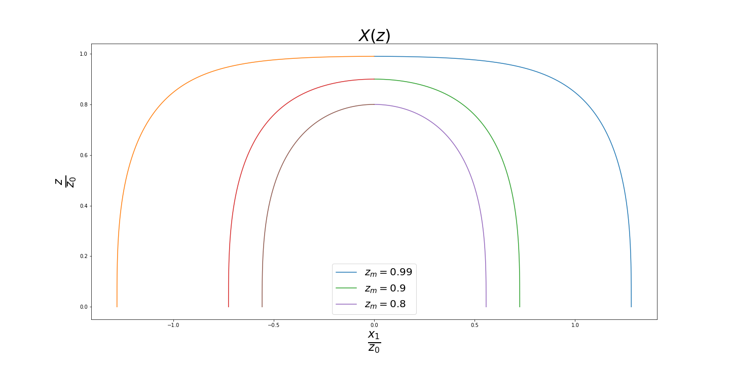
Figure 1: Confining Strings for different values of $z_{m}=Z\left(0\right)$

For numerical purposes it is convenient to parameterize the open string as

$$X\left(\sigma_{1},\sigma_{2}\right)=X(t,x_{1}):=\left(t,x_{1},0,0,Z\left(x_{1}\right)\right),$$ (19)

with this parameterization the action becomes

$$S_{B}\left[\Phi\right] =\frac{\pi z_{0}R^{3}}{4\kappa_{5}^{2}}\int dtd^{2}\bar{x}dz\left\{\left(\frac{1}{z}\right)^{3}\left(\left(\nabla_{i}\Phi\right)^{2}+f\left(z\right)\left(\partial_{z}\Phi\right)^{2}\right)\right\}$$ (20)

$$+\frac{1}{4\pi l_{s}^{2}}\int dtdx_{1}\Phi\left[X\left(x_{1}\right)\right]\sqrt{g_{E}\left(X\left(x_{1}\right)\right)}.$$ (21)

For a classical open string, using (95), the source term simplifies to

$$S_{B}\left[\Phi\right] =\frac{\pi z_{0}R^{3}}{4\kappa_{5}^{2}}\int dtd^{2}\bar{x}dz\left\{\left(\frac{1}{z}\right)^{3}\left(\left(\nabla_{i}\Phi\right)^{2}+f\left(z\right)\left(\partial_{z}\Phi\right)^{2}\right)\right\}$$ (22)

$$+\frac{z_{m}^{2}R^{2}}{4\pi l_{s}^{2}}\int dtdx_{1}\Phi\left[X\left(x_{1}\right)\right]\frac{1}{Z_{c}^{4}\left(x_{1}\right)},$$ (23)

where

$$z_{m}=Z_{c}\left(0\right).$$ (24)

We rescale the dilaton field by

$$\bar{\Phi}=\left(\frac{\pi R^{3}}{4\kappa_{5}^{2}}\right)\Phi,$$ (25)

to write the action as

$$S_{B}\left[\Phi\right] =\left(\frac{4\kappa_{5}^{2}}{\pi R^{3}}\right)\Biggl{(}z_{0}\int dtd^{2}\bar{x}dz\left\{\left(\frac{1}{z}\right)^{3}\left(\left(\nabla_{i}\Phi\right)^{2}+f\left(z\right)\left(\partial_{z}\Phi\right)^{2}\right)\right\}$$ (26)

$$+ \frac{z_{m}^{2}\lambda^{1/2}}{4\pi}\int dtdx_{1}\Phi\left[X\left(x_{1}\right)\right]\frac{1}{Z_{c}^{4}\left(x_{1}\right)}\Biggr{)}.$$ (27)

It is natural to measure the spatial coordinates in the units of $z_{0}$,

$$x_{i}\rightarrow x_{i}z_{0};\quad z\rightarrow zz_{0};\quad Z_{c}\rightarrow Z_{c}z_{0};\quad z_{m}\rightarrow z_{m}z_{0}.$$ (28)

after absorbing an overall scale factor of $\left(\frac{4\kappa_{5}^{2}}{\pi R^{3}}\right)\frac{1}{z_{0}}$ we write the dilaton action as

$$S_{B}\left[\Phi\right] =\int dtd^{2}\bar{x}dz\left\{\left(\frac{1}{z}\right)^{3}\left(\left(\nabla_{i}\Phi\right)^{2}+f\left(z\right)\left(\partial_{z}\Phi\right)^{2}\right)\right\}$$ (29)

$$+\frac{z_{m}^{2}\lambda^{1/2}}{4\pi}\int dtdx_{1}\Phi\left[X\left(x_{1}\right)\right]\frac{1}{Z_{c}^{4}\left(x_{1}\right)}.$$ (30)

It will also be useful to write the bulk action as,

$$S_{B}\left[\Phi\right]=\int dtd^{2}\bar{x}dz\left\{\left(\frac{1}{z}\right)^{3}\left(\left(\nabla_{i}\Phi\right)^{2}+f\left(z\right)\left(\partial_{z}\Phi\right)^{2}\right)+\Phi J\right\},$$ (31)

where

$$J=\frac{z_{m}^{2}\lambda^{1/2}}{4\pi}\delta(x_{2})\delta\left(z-Z_{c}\left(x_{1}\right)\right)\frac{1}{z^{4}}.$$ (32)

2.4 Classical flux-tube in $\mathrm{QCD_{3}^{W}}$

The partition function for $\mathrm{QCD_{3}^{W}}$ in the presence of a $q\bar{q}$ pair and a source term for $\widehat{\mathcal{O}}_{F^{2}}$ can be schematically written as

$$Z_{\mathrm{QCD_{3}^{W}}}[\phi]=\int[dA]\exp\left\{-S_{\mathrm{QCD_{3}^{W}}}^{q\bar{q}}[A]+2\pi r_{y}\int dtd^{2}\bar{x}\mathcal{O}_{F^{2}}\left(t,\bar{x}\right)\phi\left(t,\bar{x}\right)\right\}.$$ (33)

According to the dictionary for the gauge/gravity duality the source term $\phi\left(\bar{x}\right)$ is related to the asymptotic value of the dilaton field, again after the Kaluza-Klein reduction over the compact $y$ direction,

$$\phi\left(t,\bar{x}\right) =\lim_{z\rightarrow 0}\Phi_{c}\left(z,t,\bar{x}\right)=\lim_{z\rightarrow 0}\left(\Phi_{H}\left(z,t,\bar{x}\right)+\Phi_{s}\left(z,t,\bar{x}\right)\right),$$ (34)

$$\lim_{z\rightarrow 0} \Phi_{H}\left(z,t,\bar{x}\right)=\phi\left(t,\bar{x}\right),$$ (35)

$$\lim_{z\rightarrow 0}\Phi_{s}\left(z,t,\bar{x}\right)=0,$$ (36)

where $\Phi_{H}\left(z,t,\bar{x}\right)$ is the solution of the homogenous dilaton field equation with the boundary condition given by (35), while $\Phi_{s}\left(z,\bar{x}\right)$ is the classical dilaton field produced by the fundamental open string in the bulk. $\Phi_{H}$ is the so called non-normalizable mode while $\Phi_{s}$ is the normalizable mode. It will be convenient to write the source term in terms of the rescaled bulk field (25) and to measure the spatial coordinates $\bar{x}$ at the boundary in the units of $z_{0}=1$ (28), but we will continue to measure $\widehat{\mathcal{O}}_{F^{2}}$ in normal units in which $z_{0}\neq 1$,

$$Z_{\mathrm{QCD_{3}^{W}}}\left[\phi\right]=\int[dA]\exp\left\{-S_{\mathrm{QCD_{3}^{W}}}[A]+\pi z_{0}\left(\frac{4\kappa_{5}^{2}}{\pi R^{3}}\right)z_{0}^{2}\int dtd^{2}\bar{x}\mathcal{O}_{F^{2}}\left(t,\bar{x}\right)\phi\left(t,\bar{x}\right)\right\}.$$ (37)

Using the dictionary provided by the gauge/gravity duality in the limit $N\rightarrow\infty$ and $\lambda>>1$

$$-\frac{1}{z_{0}^{4}}\left(\frac{\delta\bar{S}}{\delta\Phi_{s}}\right)_{z=0}=\,<\Omega|\widehat{\mathcal{O}}_{F^{2}}\left(t,\bar{x}\right)|\Omega>_{q\bar{q}}.$$ (38)

Evaluating the variation about the classical solution we find that the only non-vanishing contribution comes from

$$\delta S\left[\Phi_{c}\right]=\int d^{3}x\left[\frac{2f\left(z\right)}{z^{3}}\left(\partial_{z}\Phi_{s}\right)\delta\Phi\right]_{z=z_{0}}^{z=0}.$$ (39)

Since the bulk ends smoothly at $z_{0}$, we have the following boundary condition at $z_{0}$

$$\left(\frac{\partial\Phi}{\partial z}\right)_{z=z_{0}}=0,$$ (40)

we obtain

$$<\Omega|\widehat{\mathcal{O}}_{F^{2}}\left(t,\bar{x}\right)|\Omega>_{q\bar{q}}^{X\left(\sigma\right)}=\lim_{a\rightarrow 0}\left(-\frac{1}{z_{0}^{4}}\frac{2f\left(a\right)}{a^{3}}\left(\partial_{z}\Phi_{s}\right)_{z=a}\right).$$ (41)

where the superscript $X\left(\sigma\right)$ on the left hand side is a reminder that this is the expectation value due to a particular string configuration, $X\left(\sigma\right)$, in our case the classical string configuration.

2.5 Prescription for calculating flux-profile in $\mathrm{QCD_{3}^{W}}$

Up till now we have considered a classical open string joining the quark and the antiquark as the source of the dilaton field, which in turn via (41), describes a corresponding flux-tube in the boundary theory. We will refer to the flux-tube induced by the classical open string configuration as the classical flux-tube. As was noted in the introduction, the flux-profile in the boundary theory can be thought of as a superposition of flux-tubes induced by the various string configurations making up the open string wave-function. We can formally incorporate the fluctuations of the open string by writing the partition function for the dilaton field as

$$Z_{Gravity}\left[\phi\left(\bar{x}\right)\right] =\int\left[dX\right]\exp\left\{-S_{NG}\left[X\right]\right\}\int\left[d\Phi\right]\exp\left\{-S_{B}[\Phi;X]\right\},$$ (42)

$$=\int\left[dX\right]\exp\left\{-S_{NG}\left[X\right]\right\}\exp\left\{-S_{B}\left[\Phi_{c}\left[X\right]\right]\right\},$$ (43)

where $X\left(\sigma\right)$ are the open string world sheets corresponding to strings that start at a quark and end at an antiquark, $\Phi$ represent the dilaton configurations that satisfy the boundary conditions given by (34,35,36), $S_{NG}$ is the Nambu-Goto action for an open string (6) and $S_{B}\left[\Phi;X\right]$ is the dilaton action in the presence of an open string (29). The functional integral over the dilaton field has been approximated by its classical value for $\lambda>>1$ and $N\rightarrow\infty$. Formally the flux-profile in the boundary theory can be written as

$$<\Omega|\widehat{\mathcal{O}}_{F^{2}}\left(t,\bar{x}\right)|\Omega>_{q\bar{q}} = \int\frac{\left[dX\right]}{Z_{NG}}\exp\left\{-S_{NG}\left[X\right]\right\}\left(-\frac{1}{z_{0}^{4}}\left(\frac{\delta\bar{S}}{\delta\Phi[X]}\right)_{\Phi_{c}\left(z=0,\bar{x}\right)}\right)$$ (44)

$$= \int\frac{\left[dX\right]}{Z_{NG}}\exp\left\{-S_{NG}\left[X\right]\right\}<\Omega|\widehat{\mathcal{O}}_{F^{2}}\left(t,\bar{x}\right)|\Omega>_{q\bar{q}}^{X\left(\sigma\right)}$$

where

$$Z_{NG}=\int\left[dX\right]\exp\left\{-S_{NG}\left[X\right]\right\},$$ (45)

is the partition function of the Nambu-Goto string.

We will not make an attempt to evaluate the above functional integral but will try and get a qualitatively understanding by evaluating the shape of the flux-tubes for a class of fluctuating open strings.

3 Framework for numerical calculations

To calculate the profile of the flux-tube using (41) we need to solve for the classical dilaton field, $\Phi_{c}\left(x,z\right)$, sourced by an open string. We will solve for the classical dilaton field numerically, to do so we need a discrete version of the dilaton field equation. A convenient way of doing that is by first discretizing the dilaton action RevModPhys.56.1 ; koonin1998computational .

3.1 Discretized dilaton action

Since we are working with static fields therefore it is more convenient to discretize

$$L\left[\Phi\right] =\int d^{2}\bar{x}dz\left\{\left(\frac{1}{z}\right)^{3}\left(\left(\nabla_{i}\Phi\right)^{2}+f\left(z\right)\left(\partial_{z}\Phi\right)^{2}\right)\right\}$$ (46)

$$+\frac{z_{m}^{2}\lambda^{1/2}}{4\pi}\int dx_{1}\Phi\left[X\left(x_{1}\right)\right]\frac{1}{Z_{c}^{4}\left(x_{1}\right)}.$$ (47)

Consider first the “kinetic” part of the action

$$L_{1}\left[\Phi\right]=\int_{-\infty}^{\infty}d^{2}x\int_{0}^{1}dz\left\{A\left(z\right)\left(\frac{\partial\Phi}{\partial x_{1}}\right)^{2}+A\left(z\right)\left(\frac{\partial\Phi}{\partial x_{2}}\right)^{2}+B\left(z\right)\left(\partial_{z}\Phi\right)^{2}\right\},$$ (48)

where we have defined

$$A\left(z\right)=\frac{1}{z^{3}};\quad B\left(z\right)=\frac{f\left(z\right)}{z^{3}}=\frac{\left(1-z^{4}\right)}{z^{3}}.$$ (49)

We put the system in a three-dimensional box:

$$-\frac{L_{1}}{2} \leq x_{1}\leq\frac{L_{1}}{2},$$

$$-\frac{L_{2}}{2} \leq x_{2}\leq\frac{L_{2}}{2},$$

$$0 \leq z\leq 1,$$ (50)

$L_{i}$ acting as an infrared cut-off. Next we discretize the spatial coordinates by introducing an anisotropic lattice

$$x_{i} =n_{i}b,\quad n_{i}\in\left(-N_{i},N_{i}\right),\quad L_{i}=2N_{i}b,$$

$$z =n_{3}a,\quad n_{3}\in\left(0,N_{3}\right),\quad 1=N_{3}a,$$ (51)

$$b =\sigma a,\quad\sigma>0.$$ (52)

Having an anisotropic lattice will be convenient for numerical solution of the dilaton field equation. We denote the value of the dilaton field on the points of the lattice as

$$\Phi\left(x_{1},x_{2},x_{3}\right)=\Phi\left(n_{1}b,n_{2}b,n_{3}a\right)=\Phi\left(n_{1},n_{2},n_{3}\right).$$ (53)

Now we can discretize the action (48) by calculating the integrand at the centre of the elementary cubes

$$L_{1}^{\text{lattice}}\left[\Phi\right] =\sum_{\left(n_{1,}n_{2},n_{3}\right)}b^{2}a\left\{A\left(n_{3}+1/2\right)\left(\frac{\Phi\left(n_{1}+1,n_{2},n_{3}\right)-\Phi\left(n_{1},n_{2},n_{3}\right)}{b}\right)^{2}\right.$$

$$+A\left(n_{3}+1/2\right)\left(\frac{\Phi\left(n_{1},n_{2}+1,n_{3}\right)-\Phi\left(n_{1},n_{2},n_{3}\right)}{b}\right)^{2}$$

$$\left.+B\left(n_{3}+1/2\right)\left(\frac{\Phi\left(n_{1},n_{2},n_{3}+1\right)-\Phi\left(n_{1},n_{2},n_{3}\right)}{a}\right)^{2}\right\}.$$ (54)

In terms of the scale factor $\sigma$, given by (52), the action becomes

$$L_{1}^{\text{lattice}}\left[\Phi\right] =\sum_{\left(n_{1,}n_{2},n_{3}\right)}a\left\{A\left(n_{3}+1/2\right)\left(\Phi\left(n_{1}+1,n_{2},n_{3}\right)-\Phi\left(n_{1},n_{2},n_{3}\right)\right)^{2}\right.$$

$$+A\left(n_{3}+1/2\right)\left(\Phi\left(n_{1},n_{2}+1,n_{3}\right)-\Phi\left(n_{1},n_{2},n_{3}\right)\right)^{2}$$

$$\left.+\sigma^{2}B\left(n_{3}+1/2\right)\left(\Phi\left(n_{1},n_{2},n_{3}+1\right)-\Phi\left(n_{1},n_{2},n_{3}\right)\right)^{2}\right\}.$$ (55)

The source part of the action (46) for the classical open string is

$$L_{s}=\frac{z_{m}^{2}\lambda^{1/2}}{4\pi}\int dx_{1}\Phi\left[X\left(x_{1}\right)\right]\frac{1}{Z_{c}^{4}\left(x_{1}\right)},$$ (56)

and can be discretized as

$$L_{s}^{\text{lattice}}[\Phi]=\frac{z_{m}^{2}\lambda^{1/2}}{4\pi}\sum_{n_{1}}\sigma a\left\{\Phi\left(n_{1},0,Z_{c}\left(n_{1}\right)\right)\frac{1}{Z_{c}^{4}\left(n_{1}\right)}\right\}.$$ (57)

3.2 The discrete field equation

We obtain the discrete field equation by minimizing the discrete Lagrangian

$$\frac{\partial}{\partial\Phi\left(m_{1},m_{2},m_{3}\right)}\left\{L_{1}^{\text{lattice}}+L_{s}^{\text{lattice}}\right\}=0,$$ (58)

which leads to the following discrete field equation for the dilaton field

$$\left(4A\left(m_{3}+1/2\right)+\sigma^{2}B\left(m_{3}-1/2\right)+\sigma^{2}B\left(m_{3}+1/2\right)\right)\Phi\left(m_{1},m_{2},m_{3}\right)$$

$$-A\left(m_{3}+1/2\right)\left(\Phi\left(m_{1}-1,m_{2},m_{3}\right)+\Phi\left(m_{1}+1,m_{2},m_{3}\right)\right)$$

$$-A\left(m_{3}+1/2\right)\left(\Phi\left(m_{1},m_{2}-1,m_{3}\right)+\Phi\left(m_{1},m_{2}+1,m_{3}\right)\right)$$

$$-\left(\sigma^{2}B\left(m_{3}-1/2\right)\Phi\left(m_{1},m_{2},m_{3}-1\right)+\sigma^{2}B\left(m_{3}+1/2\right)\Phi\left(m_{1},m_{2},m_{3}+1\right)\right)$$

$$+\frac{\sigma z_{m}^{2}\lambda^{1/2}}{8\pi}\left(\delta\left(0,m_{2}\right)\delta\left(Z_{c}\left(m_{1}\right),m_{3}\right)\frac{1}{Z_{c}^{4}\left(m_{1}\right)}\right) =0$$ (59)

The dilaton field equation on the lattice, (59), has to be supplemented by the boundary conditions on our box (50,51). We are interested only in the dilaton field which is sourced by the open string connecting a quark and an anti-quark, for such field we expect

$$\lim_{|\bar{x}|\rightarrow\infty}\Phi\left(\bar{x},z\right)=0.$$ (60)

On our lattice (51) this translates into

$$\Phi\left(\pm N_{1},n_{2},n_{3}\right)=0,\quad\Phi\left(n_{1},\pm N_{2},n_{3}\right)=0.$$ (61)

The bulk smoothly ends at $z_{0}$ that results in

$$\left(\frac{\partial\Phi}{\partial z}\right)_{z=z_{0}}=0,$$

which translates on our lattice as

$$\Phi\left(\bar{n},N_{3}\right)=\Phi\left(\bar{n},N_{3}-1\right).$$ (62)

Next we have to impose the boundary condition at the conformal infinity $z=0$ (36) which translates on the lattice as

$$\Phi\left(\bar{n},0\right)=0.$$ (63)

3.3 Numerical definition of the flux-tube

With all these preliminaries in place, we can translate the formula (41) on to the lattice

$$<\Omega|\widehat{\mathcal{O}}_{F^{2}}\left(\bar{n}\right)|\Omega>_{q\bar{q}}^{X\left(\sigma\right)}=-\frac{1}{z_{0}^{4}}B\left(1\right)\left(\frac{\Phi\left(\bar{n},1\right)-\Phi\left(\bar{n},0\right)}{a}\right),$$ (64)

further using the boundary condition (63) we get

$$<\Omega|\widehat{\mathcal{O}}_{F^{2}}\left(\bar{n};\right)|\Omega>_{q\bar{q}}^{X\left(\sigma\right)}=-\frac{1}{z_{0}^{4}}B\left(1\right)\left(\frac{\Phi\left(\bar{n},1\right)}{a}\right).$$ (65)

4 Shapes of confining flux-tubes

Now we are ready to numerically explore the formation of the flux-tubes in our theory. We will consider the flux-tube corresponding to the classical open string configuration, this is the flux-tube which leads to the linear confining potential for large separation of quark and anti-quark. In solving (59 ) the string-dilaton coupling

$$g_{sd}=\frac{\lambda^{1/2}}{8\pi}$$ (66)

appears only as a multiplying constant in the source term, therefore without any loss of generality we can solve the equation for an arbitrary value of $g_{sd}$. The shape of the flux-tube will be independent of the value of $g_{sd}$, the actual value of the action density will depend on $g_{sd}$ but knowing its value for a given $g_{sd}$ we can easily obtain the value for any other $g_{sd}$ by simple rescaling. In numerically solving (59) to desired precision, one faces certain number of difficulties which we point out in the appendix (C) and there we also describe the strategies we have used to overcome them.

4.1 Emergence of a classical flux-tube

We will solve the dilaton equation (59) on an anisotropic lattice with the lattice constant along the bulk direction $z$ equal to

$$a=\frac{1.0}{128}z_{0}$$ (67)

and with the lattice constant along the boundary directions $(x_{1},x_{2})$

$$b=5a=0.0390z_{0}.$$ (68)

The size of the resulting lattice is

$$V_{lattice}=128a\times 128b\times 128b=z_{0}\times 5z_{0}\times 5_{z0}$$ (69)

With such a lattice we can explore a maximum quark - antiquark distance $L_{q\bar{q}}=2.34z_{0}$, beyond that the boundary of the lattices start distorting the profile. For each value of $L_{q\bar{q}}$ the equation (59) was solved using the full multi-grid algorithm till the norm of the residue (106) was of the order $10^{-2}$ (see the accompanying python notebook, which were used to obtain the numerical results, for the details.) In delineating the shape of a flux-tube one faces the difficulty that the value of the action density diverges at the position of the quark and the anti-quark which completely masks the shape of the flux-tube. Since our interest is just to delineate and display the shape of the flux-tube we will normalize the flux-tube profile,

$$P^{X\left(\sigma\right)}\left(x_{1},x_{2}\right)=<\Omega|\widehat{\mathcal{O}}_{F^{2}}\left(x_{1},x_{2}\right)|\Omega>_{q\bar{q}}^{X\left(\sigma\right)}$$ (70)

in the following manner:

$$\text{If }P^{X\left(\sigma\right)}\left(x_{1},x_{2}\right)>P^{X\left(\sigma\right)}(x_{Lc},x_{Tc})\text{ then }P^{X\left(\sigma\right)}(x_{1},x_{2})=P^{X\left(\sigma\right)}(x_{Lc},x_{Tc}),$$ (71)

where $P^{X\left(\sigma\right)}(x_{Lc},x_{Tc})$ is the value of the flux-tube profile at the central point along the line joining the quark and the anti-quark when $L_{q\bar{q}}=2.34z_{0}$ We present the results in Figs.(2).

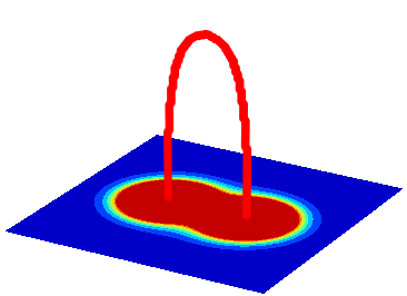
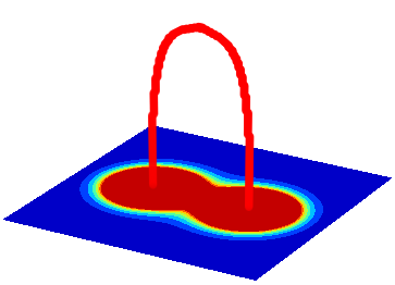
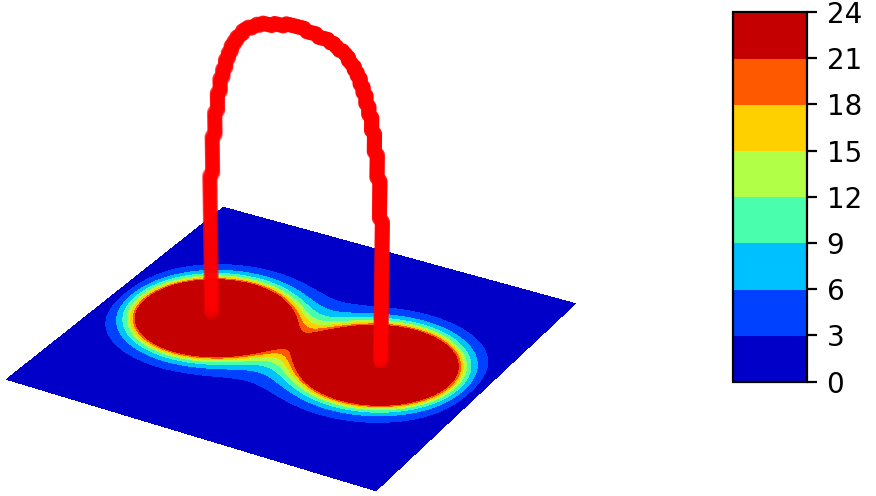
Figure 2: Normalized profile of a flux-tube with the corresponding classical open string in the bulk for $L_{q\bar{q}}=1.56\text{,\,1.95\text{ and}\,2.35}z_{0}$.

It is important to note that our results for these flux-tube profiles are only qualitative in nature as the inter quark distance is comparable to the size $r_{y}$ of the compact $y$ direction and we are averaging dilaton field over the $y$ direction. Even with this smearing of profile what we can glean is that a flux-tube starts appearing when the inter-quark distance is of the order of $3z_{0}$.

4.2 Approximate shape of a long but finite classical flux-tube

As one increases the distance between a quark and an antiquark the corresponding open string moves closer and closer to $z_{0}$, asymptotically approaching $z_{0}$. To represent such an open string on a lattice requires that the lattice constant in the $z$ direction should tend to zero or equivalently the number of points along the $z$ direction tend to infinity, making the problem computationally prohibitive. We circumvent the problem approximately by replacing the open string by a rectangular source of dilaton whose top is placed at

$$z_{Rect}^{Top}=z_{0}-a,$$ (72)

where $a$ is the lattice constant along the $z$ direction (see Fig.(3))

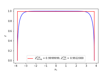
Figure 3: Open string corresponding to a long flux-tube and its approximation by a rectangular source of the dilaton field.

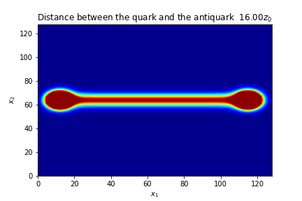
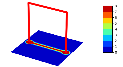
Figure 4: Long flux-tube created by a rectangular source of dilaton field

In Fig.(4) and Fig.(5)

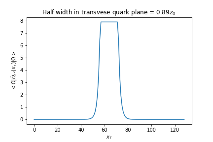
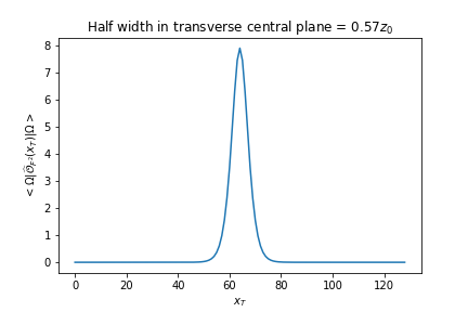
Figure 5: Thickness of a long classical flux-tube

we exhibit the flux-tube obtained using a rectangular dilaton source on an anisotropic lattice with the lattice constant $a$ along $z$ direction is

$$a=\frac{1.0}{128}z_{0}$$ (73)

and with lattice constant $b$ along the boundary directions $(x_{1},x_{2})$

$$b=20.0a.$$ (74)

The source term for rectangular open string configuration can be easily obtained using (29) and is noted in (B). As in the previous case, the dilaton field equation was solved using the full multi-grid algorithm till the norm of the residue (106) was of the order $10^{-2}$. With in the approximations that we have made, one can clearly see formation of a flux-tube with a finite intrinsic thickness.

4.3 Intrinsic thickness of an infinitely long classical flux-tube

We will next consider the situation where the quark and the anti-quark are separated by a distance much greater than $r_{y}$, or formally when

$$L_{q\bar{q}}\rightarrow\infty.$$ (75)

Gravitationally such a situation is described by an infinitely long open string placed at $z=z_{0}$. An approximate analytic solution for this case was already obtained in Danielsson:1998wt . On a lattice the profile of infinitely long open string is given by

$$Z_{c}^{\text{lattice}}\left(m_{1}\right)=Z_{c}\left(0\right)=z_{m}=aN_{m}.$$ (76)

The dilaton field sourced by such a long open string depends only on the transverse coordinate $x_{2}=am_{2}$ and on the radial coordinate $z=am_{3}$,

$$\left(2A\left(m_{3}+1/2\right)+B\left(m_{3}-1/2\right)+B\left(m_{3}+1/2\right)\right)\Phi\left(m_{2},m_{3}\right)$$

$$-A\left(m_{3}+1/2\right)\left(\Phi\left(m_{2}-1,m_{3}\right)+\Phi\left(m_{2}+1,m_{3}\right)\right)$$

$$-\left(B\left(m_{3}-1/2\right)\Phi\left(m_{2},m_{3}-1\right)+B\left(m_{3}+1/2\right)\Phi\left(m_{2},m_{3}+1\right)\right)$$

$$+\left(\frac{\lambda^{1/2}}{8\pi}\right)\frac{\delta\left(0,m_{2}\right)\delta\left(Z_{c}\left(0\right),m_{3}\right)}{Z_{c}^{2}\left(0\right)} =0.$$ (77)

We will solve the above equation numerically and use (65) to plot the intrinsic shape of the flux tube.

4.4 Numerical Results: Shape of a very long classical flux-tube

The transverse profile of a long classical flux-tube, $L_{q\bar{q}}\rightarrow\infty$, can be defined as

$$P_{T}^{X_{c}\left(\sigma\right)}\left(x_{T}\right)=\lim_{L_{q\bar{q}}\rightarrow\infty}<\Omega|\widehat{\mathcal{O}}_{F^{2}}\left(x_{1}=0;x_{2}=x_{T}\right)|\Omega>_{q\bar{q}}^{X_{c}\left(\sigma\right)}.$$ (78)

If the flux-tube is formed because of the finite correlation-length of flux-lines, as suggested in Wilson:1977nj , then we expect that the transverse profile should take the following form

$$\lim_{|x_{T}|\rightarrow\infty}P_{T}\left(x_{T}\right)=C_{0}\exp\left(-\frac{|x_{T}|}{\xi_{FT}}\right)=C_{0}\exp\left(-|x_{T}|M_{\text{glueball}}^{-1}\right),),$$ (79)

where $C_{0}$ is a constant of mass dimension four and $\xi_{FT}$ is the correlation length of the flux-lines (see the discussion in section 2 of Wilson:1977nj ) and is a measure of the intrinsic thickness of the flux-tube. The inverse of $\xi_{FT}$ is, on dimensional grounds, related to the lightest glueball mass.

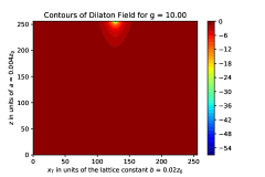
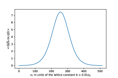
Figure 6: Dilaton field due to a infinitely long open string along the $x_{1}$ axis and the resulting confining flux-tube on the boundary.

The results of numerical calculations are presented in Fig.(6) and more detailed description of fitting of the data with a Gaussian and an exponential function is provided in Fig.(7). Because of the two dimensional nature of the problem the dilaton field equation could be solved with great precision, norm of the residue (107) being of the order of $10^{-6}$.

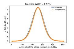
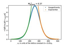
Figure 7: Intrinsic shape of a infinitely long confining flux-tube and its fit to an exponential and Gaussian function

$L_{q\bar{q}}$	Half width along the line $x_{1}=L_{q\bar{q}}/2$
1.56	0.65
1.95	0.61
2.34	0.58
$16.00\text{ rect. string}$	0.57
$\infty$	0.57

Table 1: Half width of the normalized profile in units of $z_{0}$ for different values of $L_{q\bar{q}}$.

In Table(1) we summarize the relationship between the thickness and length of a classical flux-tube. The table clearly indicates that as the distance between the quark and the anti-quark, $L_{q\bar{q}}$, is increased a flux-tube is formed with a width which is asymptotically independent of $L_{q\bar{q}}$.

4.5 Flux-tube with fluctuating thickness

From the very inception of the gauge/gravity duality it was recognized that the position of an object along the extra radial direction is related to the size of it’s holographic projection in the boundary theory Susskind:1998dq . For a confining theories this suggests that the size of the flux-tube must be related to the position of the corresponding open string in bulk. Further an open string with a fluctuating radial coordinate along the extra dimension will correspond to a flux-tube with varying thickness. We will verify that this is indeed the case for $\mathrm{QCD_{3}^{W}}$. We do so by considering an open rectangular string, like the one we considered in section (4.2), on which we superimpose random fluctuations along the $z$ direction and then calculate the profile of the corresponding flux-tube. We present the result in Fig.(8).

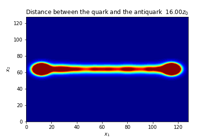
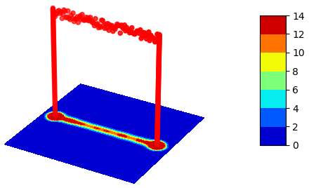
Figure 8: Static radially fluctuating open string and the corresponding flux-tube

5 Discussion

It is natural to ask, is there any thing that we can learn about real QCD from the toy example considered in the present work. There are few ways in which the phenomena that we have explored can get reflected in QCD. Firstly QCD flux-tubes should have an intrinsic thickness which can fluctuate. These radial fluctuations should lead to an attractive Yukawa like potential Kinar:1999xu and it might be interesting to incorporate these fluctuations in the effective string models of the fragmentation of hadrons BERENYI2015210 .

The shape of the flux-tubes (see Figs.(2, 4) and Table (1)) suggests that in an effective string description of QCD flux-tube the string tension should depend on the distance between the quark and the anti-quark and approaches its constant value only as that distance tends to infinity Nielsen:1973cs ; Vyas:2010uq . This would imply that when the distance between the quark and the anti-quark is of the order of the confinement scale then there should be deviations from the heavy quark potential calculated using an infinitely long open string Aharony:2010db ; Aharony:2010cx . For in this regime the open string in the gravitational description is not an infinitely long open string placed at the confinement scale but has to descent to the conformal boundary. In the boundary theory this is reflected in the fact that when the quark anti-quark distance is of the order of the confinement scale then the size of the blob of action density surrounding the quark and the antiquark is comparable to the distance between the quark and the anti-quark. A preliminary estimate of this effect was made in Vyas:2012fk but a more precise calculation and its comparison with a high precision lattice simulations like Brandt:2017aa should be revealing.

Another place where the intrinsic shape of a confining flux-tube can have a physical consequences is in the possible presence of a long range spin-spin interaction term in the heavy quark potential. In Kogut:1981gm it was argued, using the analogy with $U(1)$ gauge theories, that the quantum fluctuations of an electric flux-tube will induce a magnetic field which will couple the spins of the quark and the anti-quark leading to a spin-spin dependent potential term which falls as the fifth power of the distance between the quark and the anti-quark. In Vyas:2007bi this was analysed using an effective string description for the expectation value of a spin-half Wilson Loop. It was found that for an effective string with Dirichlet boundary conditions there is no spin-spin dependent potential term, but when an allowance was made for the intrinsic thickness of the flux-tube near the end points, by calculating the spin-string interaction not at the end points but at a finite distance away from the end points, then a spin-spin interaction was indeed obtained. The shape of the confining flux-tube that we have obtained in the present investigation gives some credence to the analysis of Vyas:2007bi , for the flux-tubes that are induced in the boundary theory do not terminate at the position of the quark or the anti-quark, rather they extend beyond it. We do not know how to incorporate this feature of the confining flux-tubes in an effective string description (the analysis of Vyas:2007bi is physically motivated but ad-hoc), perhaps the analysis of boundary conditions in the context of holographic stringy description of hadrons Sonnenschein:2016aa ; Sonnenschein:2017ylo , and the analysis of the boundary conditions of an open string in the bulk under holographic renormalization group Casalderrey-Solana:2019vnc may provide us with some guidance.

Appendix A Shape of the open string sourcing the dilaton field

The shape of the classical open string connecting the quark to the anti-quark can be obtained from

$$S_{NG}[X\left(\sigma\right)]=\frac{1}{2\pi\alpha^{\prime}}\int d^{2}\sigma\sqrt{g_{E}\left(X\right)}.$$ (80)

We parameterize the world-sheet as

$$X\left(t,x\right):=\left(t,x_{1}=x,x_{2},y,Z\left(x\right)\right).$$ (81)

Using the metric (7) we obtain the induced world-sheet metric for an open string lying in the $x_{1}-z$ plane as

$$g_{ab}=\text{diag}\left\{\left(\frac{R}{Z}\right)^{2},\left(\frac{R}{Z}\right)^{2}\left(1+\frac{1}{f\left(z\right)}\left(\frac{dZ}{dx}\right)^{2}\right)\right\},$$ (82)

where

$$f\left(z\right)=\left(1-\left(\frac{z}{z_{0}}\right)^{4}\right).$$ (83)

The parametrized Nambu-Goto action then takes the form

$$S_{NG}\left[X\right]=\frac{R^{2}}{2\pi\alpha^{\prime}}\int dtdx\left\{\frac{1}{Z\left(x\right)^{2}}\left(1+\frac{1}{f\left(z\right)}\left(\frac{dZ}{dx}\right)^{2}\right)^{1/2}\right\}.$$ (84)

Following Kinar:1998vq we note that the action does not depend explicitly on $t$ therefore for the time interval $\left(-T/2,T/2\right)$ it can be written as

$$S_{NG}^{0}=\int_{-L/2}^{L/2}dx_{1}L\left(Z,Z^{\prime}\right),$$

where

$$L\left(Z,Z^{\prime}\right)=C_{0}\frac{1}{Z^{2}}\left(1+\frac{1}{f\left(z\right)}\left(\frac{dZ}{dx_{1}}\right)^{2}\right)^{1/2}$$ (85)

and we have defined the constant

$$C_{0}=\frac{TR^{2}}{2\pi\alpha^{\prime}}.$$ (86)

$L$ describes a one-dimensional problem with $x_{1}$ playing the role of time parameter, since $L$ does not depend explicitly on $x_{1}$ there is a conserved quantity

$$H=P\frac{dZ}{dx_{1}}-L=PZ^{\prime}-L,$$ (87)

where the momentum conjugate to $Z$ is given by

$$P=\frac{\partial L}{\partial\left(\frac{dZ}{dx_{1}}\right)}=\frac{\partial L}{\partial Z^{\prime}}.$$ (88)

Using the above equations we obtain

$$H=\frac{-C_{0}}{Z^{2}\left(1+\frac{1}{f\left(Z\right)}\left(\frac{dZ}{dx_{1}}\right)^{2}\right)^{1/2}},$$ (89)

which is conserved

$$\frac{dH}{dx_{1}}=0.$$ (90)

By symmetry

$$\left(\frac{dZ}{dx_{1}}\right)_{x_{1}=0}=0,$$ (91)

let

$$Z\left(0\right)=z_{m}.$$ (92)

Conservation of $H$ allows us to write

$$\frac{1}{Z^{2}\left(1+\frac{1}{f\left(Z\right)}\left(\frac{dZ}{dx_{1}}\right)^{2}\right)^{1/2}}=\frac{1}{z_{m}^{2}},$$ (93)

and we can obtain an equation for $Z\left(x_{1}\right)$

$$\frac{dZ}{dx_{1}}=\pm\sqrt{f\left(z\right)\left(\left(\frac{z_{m}}{Z}\right)^{4}-1\right)}$$ (94)

the $\pm$ signs corresponding to the left and the right part of the string that connects a quark at $-L/2$ to an anti-quark at $L/2$. Using above result we can calculate

$$\sqrt{g_{E}\left(Z_{c}\right)}=\frac{1}{Z\left(x\right)^{2}}\left(1+\frac{1}{f\left(z\right)}\left(\frac{dZ}{dx}\right)^{2}\right)^{1/2}=R^{2}\frac{z_{m}^{2}}{Z\left(x\right)^{4}}$$ (95)

Next consider the positive branch of (94), and noting that $Z\left(x_{1}\right)$ is an invertible function, we obtain

$$\frac{dX_{1}}{dz}=\left(f\left(z\right)\left(\left(\frac{z_{m}}{Z}\right)^{4}-1\right)\right)^{-1/2},$$ (96)

which is more convenient for numerical calculations.

Appendix B Dilaton source term due to a rectangular string

The dilaton string coupling for a static string configuration is given by

$$S_{ds}\left[X\left(\sigma\right)\right]=\frac{1}{4\pi l_{s}^{2}}\int dtd\sigma\Phi\left[X\left(\sigma\right)\right]\sqrt{g_{E}\left(X\left(\sigma\right)\right)}.$$ (97)

For a rectangular source of a dilaton field (3) we will parametrize the two sides of the rectangle by $\sigma=z,$and obtain

$$S_{\text{Rect. side}}=\frac{\lambda^{1/2}}{4\pi}\int dtdz\Phi\left[X\left(z\right)\right]\frac{1}{z^{2}\left(1-z^{4}\right)^{1/2}},$$ (98)

with

$$X\left(\sigma\right):=\left(t,x_{1q},0,0,z\right).$$ (99)

For the top of the rectangle we use $\sigma=x_{1}$ as the parameter,

$$S_{\text{Rect. top}}=\frac{\lambda^{1/2}}{4\pi}\int dtdx_{1}\Phi\left[X\left(x_{1}\right)\right]\frac{1}{Z^{2}}\left(1+\frac{1}{\left(1-Z^{4}\right)}\left(\frac{dZ}{dx_{1}}\right)^{2}\right)^{1/2},$$ (100)

where the string profile is given by

$$X\left(\sigma\right):=\left(t,x_{1},0,0,Z\left(x_{1}\right)\right).$$ (101)

Appendix C Numerical solution of the dilaton field equation

The discrete version of the dilaton field equation (59) can be solved using relaxation algorithm koonin1998computational

$$\Phi(m_{1},m_{2},m_{3})\rightarrow\left(1-\omega\right)\Phi\left(m_{1},m_{2},m_{3}\right)\\ +\frac{\omega}{C\left(m_{3}\right)}(A_{m_{3}+1/2}(\Phi\left(m_{1}-1,m_{2},m_{3}\right)+\Phi\left(m_{1}+1,m_{2},m_{3}\right)\\ +\Phi\left(m_{1},m_{2}-1,m_{3}\right)+\Phi\left(m_{1},m_{2}+1,m_{3}\right))\\ +\frac{\omega}{C\left(m_{3}\right)}\left(\sigma^{2}B_{m_{3}-1/2}\Phi\left(m_{2},m_{3}-1\right)+\sigma^{2}B_{m_{3}+1/2}^{2}\Phi\left(m_{2},m_{3}+1\right)\right)\\ -\frac{\omega}{C\left(m_{3}\right)}\frac{\sigma z_{m}^{2}\lambda^{1/2}}{8\pi}\left(\delta\left(0,m_{2}\right)\delta\left(Z_{c}\left(m_{1}\right),m_{3}\right)\frac{1}{Z_{c}^{4}\left(m_{1}\right)}\right),$$ (102)

with $C\left(m_{3}\right)$ defined as

$$C\left(m_{3}\right)=4A+\sigma^{2}B_{m_{3}-1/2}+\sigma^{2}B_{m_{3}+1/2},$$

and $\omega$ is the relaxation parameter.

For the two dimensional case discussed in sec.(4.3) the discrete version of the dilaton field equation (77) can be solved by the following relaxation procedure koonin1998computational , setting $\sigma=1,$

$$\Phi(m_{2},m_{3})=\left(1-\omega\right)\Phi\left(m_{2},m_{3}\right)\\ +\frac{\omega}{C\left(m_{3}\right)}\left(A_{m_{3}+1/2}\left(\Phi\left(m_{2}-1,m_{3}\right)+\Phi\left(m_{2}+1,m_{3}\right)\right)\right)\\ +\frac{\omega}{C\left(m_{3}\right)}\left(B_{m_{3}-1/2}\Phi\left(m_{2},m_{3}-1\right)+B_{m_{3}+1/2}\Phi\left(m_{2},m_{3}+1\right)\right)\\ -\frac{\omega}{C\left(m_{3}\right)}\left(\frac{\lambda^{1/2}}{8\pi}\frac{\delta_{0,m_{2}}\delta_{N_{m},m_{3}}}{Z_{\text{lattice}}^{2}\left(0\right)}\right),$$ (103)

where

$$C\left(m_{3}\right)=2A_{m_{3}+1/2}+B_{m_{3}-1/2}+B_{m_{3}+1/2}$$

and $\omega$ is again the relaxation parameter.

In using relaxation algorithm one encounters the problem of critical slowing down, namely that the long wavelength part of the solution takes very large number of iterations to relax to its true value, the number of iterations diverging as the size of the lattice increases. For example if we consider a linear problem

$$L\mathbf{u}=\mathbf{s},$$ (104)

with a given source vector $\mathbf{s}$ and tries to solve for the vector $\mathbf{u}$ using a relaxation algorithm then one finds that the norm of the residue vector

$$\mathbf{r}=\mathbf{s}-L\mathbf{u},$$ (105)

initially decreases with the number of iterations but after a while it stops reducing. To mitigate the problem of critical slowing down we used multigrid algorithm trottenberg2001multigrid ; stewart2017python .

For the case of three dimensional anisotropic lattice we used the following definition of the norm

$$\left\|\mathbf{r}\right\|=\sqrt{\left(a*b^{2}\mathbf{r}\cdot\mathbf{r}\right)},$$ (106)

where $a$ is the lattice constant along the $z$ direction while $b$ is the lattice constant along $x_{1}$ and $x_{2}$ direction. For the two dimensional case with an isotropic lattice constant $a$ the norm was taken to be

$$\left\|\mathbf{r}\right\|=\sqrt{\left(a^{2}\mathbf{r}\cdot\mathbf{r}\right)}$$ (107)

All the numerical calculations involved in this work were done using python 3.0 JupyterLab notebooks which are included as supplemental material. Easiest way to run these notebooks is to install free and open-source python distribution like Anaconda. The four notebooks included as ancillary files in the ArXiv submission are:

1. ShapeOfFluxTube-1.ipynb which was used for the calculations reported in section (4.1). This notebook depends on two python files

   1. utility_3DimMG.py

   2. AiStringSource.py

2. RectangularString.ipynb which was used for calculations reported in section (4.2). This notebook depends on the python file

   1. utility_3DimMG.py

3. ShapeOfFluxTube-3.ipynb which was used for calculations reported in section (4.4). This notebook depends on the python file

   1. utility_2DimMG.py

4. flucRectString.ipynb which was used for the calculations reported in section (4.5).This notebook depends on the python file

   1. utility_2DimMG.py

References

- (1) V. Singh, D. Browne, and R. Haymaker, Structure of abrikosov vortices in su(2) lattice gauge theory, Physics Letters B 306 (May, 1993) 115–119, [hep-lat/9301004].
- (2) G. S. Bali, K. Schilling, and C. Schlichter, Observing long color flux tubes in su(2) lattice gauge theory, Phys. Rev. D51 (1995) 5165–5198, [hep-lat/9409005].
- (3) F. Bissey, A. I. Signal, and D. B. Leinweber, Comparison of gluon flux-tube distributions for quark-diquark and quark-antiquark hadrons, Phys.Rev.D 80 (2009) 114506, [arXiv:0910.0958].
- (4) Y. Nambu, Strings, monopoles, and gauge fields, Phys. Rev. D 10 (Dec, 1974) 4262–4268.
- (5) G. ’t Hooft, A Property of Electric and Magnetic Flux in Nonabelian Gauge Theories, Nucl. Phys. B153 (1979) 141–160.
- (6) S. Mandelstam, General introduction to confinement, Physics Reports 67 (1980), no. 1 109 – 121.
- (7) K. G. Wilson, Quantum chromodynamics on a lattice, 1977. Presented at Cargese Summer Institute, Cargese, France, Jul 12- 31, 1976.
- (8) R. P. Feynman, The qualitative behavior of yang-mills theory in 2 + 1 dimensions, Nuclear Physics B 188 (1981), no. 3 479 – 512.
- (9) P. Cea, L. Cosmai, and A. Papa, Chromoelectric flux tubes and coherence length in QCD, Phys. Rev. D86 (2012) 054501, [arXiv:1208.1362].
- (10) N. Cardoso, M. Cardoso, and P. Bicudo, Inside the su(3) quark-antiquark qcd flux tube: screening versus quantum widening, [arXiv:1302.3633].
- (11) M. Caselle, M. Panero, and D. Vadacchino, Width of the flux tube in compact u(1) gauge theory in three dimensions, [arXiv:1601.0745].
- (12) P. Cea, L. Cosmai, F. Cuteri, and A. Papa, Flux tubes in the QCD vacuum, Phys. Rev. D95 (2017), no. 11 114511, [arXiv:1702.0643].
- (13) M. Baker, P. Cea, V. Chelnokov, L. Cosmai, F. Cuteri and A. Papa, Spatial structure of the color field in the SU(3) flux tube, PoS LATTICE 2018, 253 (2018) [arXiv:1811.00081]
- (14) J. M. Maldacena, The large N limit of superconformal field theories and supergravity, Adv. Theor. Math. Phys. 2 (1998) 231, [hep-th/9711200].
- (15) S. S. Gubser, I. R. Klebanov, and A. M. Polyakov, Gauge theory correlators from non-critical string theory, Phys. Lett. B428 (1998) 105--114, [hep-th/9802109].
- (16) E. Witten, Anti-de Sitter space and holography, Adv.Theor.Math.Phys. 2 (1998) 253--291, [hep-th/9802150].
- (17) E. Witten, Anti-de sitter space, thermal phase transition, and confinement in gauge theories, Adv. Theor. Math. Phys. 2 (1998) 505--532, [hep-th/9803131].
- (18) J. M. Maldacena, Tasi 2003 lectures on ads/cft, hep-th/0309246.
- (19) A. M. Polyakov, String theory and quark confinement, Nucl. Phys. Proc. Suppl. 68 (1998) 1, [hep-th/9711002].
- (20) J. M. Maldacena, Wilson loops in large n field theories, Phys. Rev. Lett. 80 (1998) 4859, [hep-th/9803002].
- (21) S. J. Rey and J. T. Yee, Macroscopic strings as heavy quarks in large N gauge theory and anti-de Sitter supergravity, Eur. Phys. J. C22 (2001) 379, [hep-th/9803001].
- (22) V. Balasubramanian, P. Kraus, and A. Lawrence, Bulk vs. boundary dynamics in anti-de sitter spacetime, hep-th/9805171.
- (23) V. Balasubramanian, P. Kraus, A. E. Lawrence, and S. P. Trivedi, Holographic probes of anti-de Sitter space-times, Phys. Rev. D59 (1999) 104021, [hep-th/9808017].
- (24) U. H. Danielsson, E. K. Vakkuri, and E. Kruczenski, Vacua, Propagators, and Holographic Probes in AdS/CFT, JHEP 01 (1999) 002, [hep-th/9812007].
- (25) C. G. Callan, Jr. and A. Guijosa, Undulating strings and gauge theory waves, Nucl. Phys. B 565, 157 (2000), [hep-th/9906153]
- (26) J. Polchinski and L. Susskind, String theory and the size of hadrons, [hep-th/0112204].
- (27) D. Giataganas and N. Irges, On the holographic width of flux tubes, JHEP 1505, 105 (2015), [arXiv:1502.05083].
- (28) Y. Kinar, E. Schreiber, and J. Sonnenschein, Q anti-q potential from strings in curved spacetime: Classical results, Nucl. Phys. B566 (2000) 103, [hep-th/9811192].
- (29) A. M. Polyakov, Gauge Fields and Strings. Contemporary concepts in physics. Taylor & Francis, 1987.
- (30) M. Ammon and J. Erdmenger, Gauge/Gravity Duality. Cambridge University Press, 2015.
- (31) D. Tong, Lectures on string theory, [arXiv:0908.0333].
- (32) S. L. Adler and T. Piran, Relaxation methods for gauge field equilibrium equations, Rev. Mod. Phys. 56 (Jan, 1984) 1--40.
- (33) S. Koonin and D. Meredith, Computational Physics: Fortran Version. Addison-Wesley, 1998.
- (34) U. Kol and J. Sonnenschein, Can holography reproduce the QCD Wilson line? JHEP 1105, 111 (2011), [1012.5974].
- (35) L. Susskind and E. Witten, The holographic bound in anti-de Sitter space, [hep-th/9805114].
- (36) Y. Kinar, E. Schreiber, J. Sonnenschein, and N. Weiss, Quantum fluctuations of Wilson loops from string models, Nucl. Phys. B583 (2000) 76, [hep-th/9911123].
- (37) D. Berényi, S. Varró, V. V. Skokov, and P. Lévai, Pair production at the edge of the qed flux tube, Physics Letters B 749 (2015) 210 -- 214, [arXiv:1401.0039]
- (38) H. B. Nielsen and P. Olesen, Vortex-line models for dual strings, Nucl. Phys. B61 (1973) 45.
- (39) V. Vyas, Intrinsic thickness of qcd flux-tubes, [arXiv:1004.2679].
- (40) O. Aharony and N. Klinghoffer, Corrections to Nambu-Goto energy levels from the effective string action, JHEP 1012 (2010) 058, [arXiv:1008.2648].
- (41) O. Aharony and M. Field, On the effective theory of long open strings, JHEP 1101 (2011) 065, [arXiv:1008.2636].
- (42) V. Vyas, Heavy quark potential from gauge/gravity duality: A large d analysis, Phy. Rev. D 87 (09, 2013) 045026, [arXiv:1209.0883].
- (43) B. B. Brandt, Spectrum of the open qcd flux tube and its effective string description i: 3d static potential in su(n=2,3), [arXiv:1705.0382].
- (44) J. B. Kogut and G. Parisi, Long Range Spin Spin Forces in Gauge Theories, Phys. Rev. Lett. 47, 1089 (1981).
- (45) V. Vyas, Spin-string interaction in QCD strings, Phys. Rev. D 78, 045003 (2008), [arXiv:0704.2707].
- (46) J. Sonnenschein, Holography inspired stringy hadrons, [arXiv:1602.0070].
- (47) J. Sonnenschein and D. Weissman, The decay width of stringy hadrons, Nucl. Phys. B 927 (2018) 368, [arXiv:1705.10329].
- (48) J. Casalderrey-Solana, D. Gutiez and C. Hoyos, JHEP 1904 (2019) 134, [arXiv:1902.04279].
- (49) U. Trottenberg, C. Oosterlee, and A. Schuller, Multigrid. Elsevier Science, 2001.
- (50) J. Stewart, Python for Scientists. Cambridge University Press, 2017.