Data-driven Decision Making with Probabilistic Guarantees (Part II):
Applications of Chance-constrained Optimization in Power Systems

Abstract

Uncertainties from deepening penetration of renewable energy resources have posed critical challenges to the secure and reliable operations of future electric grids. Among various approaches for decision making in uncertain environments, this paper focuses on chance-constrained optimization, which provides explicit probabilistic guarantees on the feasibility of optimal solutions. Although quite a few methods have been proposed to solve chance-constrained optimization problems, there is a lack of comprehensive review and comparative analysis of the proposed methods. Part I of this two-part paper reviews three categories of existing methods to chance-constrained optimization: (1) scenario approach; (2) sample average approximation; and (3) robust optimization based methods. Data-driven methods, which are not constrained by any particular distributions of the underlying uncertainties, are of particular interest. Part II of this two-part paper provides a literature review on the applications of chance-constrained optimization in power systems. Part II also provides a critical comparison of existing methods based on numerical simulations, which are conducted on standard power system test cases.

About

• This is Part 2 of a two-part review paper titled “Data-driven Decision Making in Power Systems with Probabilistic Guarantees: Theory and Applications of Chance-constrained Optimization” by Xinbo Geng and Le Xie, Annual Reviews in Control (under review).

• Part 1 “Data-driven Decision Making with Probabilistic Guarantees (Part I): A Schematic Overview of Chance-constrained Optimization” is available at arXiv:1903.10621.

• Part 2 “Data-driven Decision Making in with Probabilistic Guarantees (Part II): Applications of Chance-constrained Optimization in Power Systems” is available at arXiv.

• The Matlab Toolbox ConvertChanceConstraint (CCC) is available at https://github.com/xb00dx/ConvertChanceConstraint-ccc.

Please let us know if we missed any critical references or you found any mistakes in the manuscript.

Recent Updates

04/2019

Part II uploaded to Arxiv.

04/2019

More CVaR-based (Convex Approximation) results are added in Part 1.

02/2019

Toolbox published at https://github.com/xb00dx/ConvertChanceConstraint-ccc. We are still working on the toolbox website and documents.

1 Introduction

Real-time decision making in the presence of uncertainties is a classical problem that arises in many contexts. In the context of electric energy systems, a pivotal challenge is how to operate a power grid with an increasing amount of supply and demand uncertainties. The unique characteristics of such operational problem include (1) the underlying distribution of uncertainties is largely unknown (e.g. the forecast error of demand response); (2) decisions have to be made in a timely manner (e.g. a dispatch order needs to be given by 5 minutes prior to the real-time); and (3) there is a strong desire to know the risk that the system is exposed to after a decision is made (e.g. the risk of violating transmission constraints after the real-time market clears). In response to these challenges, a class of optimization problems named “chance-constrained optimization” has received increasing attention in both operations research and practical engineering communities.

The objective of this article is to provide a comprehensive and up-to-date literature review on the engineering implications of chance-constrained optimization in the context of electric power systems.

1.1 Contributions of This Paper

The main contributions of this paper are threefold:

1. We provide a detailed tutorial on existing algorithms to solve chance-constrained programs and a survey of major theoretical results. To the best of our knowledge, there is no such review available in the literature;

2. We provide a comprehensive review on the applications of chance-constrained optimization in power systems, with focus on various interpretations of chance constraints in the context of power engineering.

3. We implement all the reviewed methods and develop an open-source Matlab toolbox (ConvertChanceConstraint), which is available on Github . We also provide a critical comparison of existing methods based numerical simulations on IEEE standard test systems.

1.2 Organization of This Paper

The remainder of this paper is organized as follows. Section 2 provides a comprehensive review on applications of CCO in power systems. The structure and usage of the Toolbox ConvertChanceConstraint is in Section 3. Section 3 also conducts numerical simulations and compares existing approaches to solving CCO problems. Concluding remarks are in Section 4.

1.3 Notations

The notations in this paper are standard. All vectors and matrices are in the real field $\mathbf{R}$. Sets are in calligraphy fonts, e.g. $\mathcal{S}$. The upper and lower bounds of a variable $x$ are denoted by $\overline{x}$ and $\underline{x}$. The estimation of a random variable $\epsilon$ is $\hat{\epsilon}$. We use $\mathbf{1}_{n}$ to denote an all-one vector in $\mathbf{R}^{n}$, the subscript $n$ is sometimes omitted for simplicity. The absolute value of vector $x$ is $|x|$, and the cardinality of a set $\mathcal{S}$ is $|\mathcal{S}|$. Function $[a]_{+}$ returns the positive part of variable $a$. The indicator function $\mathbbm{1}_{x>0}$ is one if $x>0$. The floor function $\left\lfloor a\right\rfloor$ returns the largest integer less than or equal to the real number $a$. The ceiling function $\left\lceil a\right\rceil$ returns the smallest integer greater than or equal to $a$. $\mathbb{E}[\xi]$ is the expectation of a random vector $\xi$, $\mathbb{V}(x)$ denotes the violation probability of a candidate solution $x$, and $\mathbb{P}_{\xi}(\cdot)$ is the probability taken with respect to $\xi$. The transpose of a vector $a$ is $a^{\intercal}$. Infimum, supremum and essential supremum are denoted by $\inf$, $\sup$ and $\operatorname*{ess\,sup}$. The element-wise multiplication of the same-size vectors $a$ and $b$ is denoted by $a\circ b$.

2 Applications in Power Systems

A pivotal task in modern power system operation is to maintain the real-time balance of supply and demand while ensuring the system is low-cost and reliable. This pivotal task, however, faces critical challenges in the presence of rapid growth of renewable energy resources. Chance-constrained optimization, which explicitly models the risk that the system is exposed to, is a suitable conceptual framework to ensure the security and reliability of a power system under uncertainties.

There is a large body of literature adopting CCO for power system applications. Figure 1 presents some existing applications of CCO in power systems. In the following sections, we introduce three important applications of CCO in power systems: security-constrained economic dispatch (SCED) (Section 2.1), security-constrained unit commitment (SCUC) (Section 2.2) and generation and transmission expansion (Section 2.3).

Figure 1 also presents a feed-forward decision making framework for power system operations. The feed-forward framework partitions the overall decision making process into several time segments. The longer-term decisions (e.g. generation expansion) are fed into shorter-term decision making processes (e.g. unit commitment). The shorter-term decisions (e.g. generation commitment from SCUC) have direct impacts on real-time operations (e.g. dispatch results in SCED). It is worth noting that as time draws closer to the actual physical operation, information gets much sharper (Xie et al., 2011).

Figure 1: Representative feed-forward decisions made in power system planning and operation

Table 1: Power System Applications of Chance-constrained Optimization

Deterministic Equivalent
Scenario Approach
Sample Average Approximation
RO-based Approach
Others

2.1 Security-Constrained Economic Dispatch

2.1.1 Deterministic SCED

Security-constrained Economic Dispatch (SCED) lies at the center of modern electricity markets and short-term power system operations. It determines the most cost-efficient output levels of generators while keeping the real-time balance between supply and demand. Different variations of the SCED problem are all based on the direct current optimal power flow (DCOPF) problem. We present a typical form of DCOPF with wind generation.

$$\text{(det-DCOPF):}~{}\min_{g}~{} c(g)$$ (1a)

s.t $$\mathbf{1}^{\intercal}g=\mathbf{1}^{\intercal}d-\mathbf{1}^{\intercal}\hat{w}$$ (1b)

$$f=H_{g}g+H_{w}\hat{w}-H_{d}d$$ (1c)

$$\underline{f}\leq f\leq\overline{f}$$ (1d)

$$\underline{g}\leq g\leq\overline{g}$$ (1e)

The decision variables are generation output levels $g\in\mathbf{R}^{n_{g}}$. The objective of (det-DCOPF) is to minimize total generation cost $c(g)$, while ensuring total generation equates total net demand (1b). Constraints include transmission line flow limits (1c)-(1d) and generation capacity limits (1e). Transmission line flows $f\in\mathbf{R}^{n_{l}}$ are calculated using (1c), in which $H$ is the power transfer distribution factor (PTDF) matrix, and $H_{g}\in\mathbf{R}^{n_{l}\times n_{g}}$ ($H_{d}\in\mathbf{R}^{n_{l}\times n_{d}}$,$H_{w}\in\mathbf{R}^{n_{l}\times n_{w}}$) denotes the submatrix formed by the columns of $H$ corresponding to generators (loads, wind farms). (1) utilizes the expected wind generation or wind forecast $\hat{w}$, we refer to (1) as deterministic DCOPF (det-DCOPF) since no uncertainties are being considered.

2.1.2 Chance-constrained SCED

Many researchers advance (det-DCOPF) towards a chance-constrained formulation with wind uncertainties. A representative formulation is (2), which appears in a majority of the existing literatures, e.g. (Bienstock et al., 2014; Vrakopoulou et al., 2013a).

(cc-DCOPF):

$$\min_{g,\eta}~{} c(g)$$ (2a)

s.t $$\mathbf{1}^{\intercal}g=\mathbf{1}^{\intercal}d-\mathbf{1}^{\intercal}\hat{w}$$ (2b)

$$f(\hat{w},\tilde{w})=H_{g}(g-\mathbf{1}^{\intercal}\tilde{w}\eta)$$

$$\hskip 40.0pt-H_{d}d+H_{w}(\hat{w}+\tilde{w})$$ (2c)

$$\mathbb{P}_{\tilde{w}}\Big{(}\underline{f}\leq f(\hat{w},\tilde{w})\leq\overline{f}~{}\text{and}$$

$$\hskip 15.0pt\underline{g}\leq g-\mathbf{1}^{\intercal}\tilde{w}\eta\leq\overline{g}\Big{)}\geq 1-\epsilon$$ (2d)

$$\mathbf{1}^{\intercal}\eta=1$$ (2e)

$$\underline{g}\leq g\leq\overline{g}$$ (2f)

$$-\mathbf{1}\leq\eta\leq\mathbf{1}$$ (2g)

Unlike (det-DCOPF) using wind forecast $\hat{w}$, chance-constrained SCED (cc-DCOPF) explicitly models wind generation as a random vector $w\in\mathbf{R}^{n_{w}}$. The wind generation $w=\hat{w}+\tilde{w}$ is decomposed into two components: the deterministic wind forecast value $\hat{w}\in\mathbf{R}^{n_{w}}$ and the uncertain forecast error $\tilde{w}\in\mathbf{R}^{n_{w}}$. To guarantee the real-time balance of supply and demand, (cc-DCOPF) introduces an affine control policy $\eta\in[-1,1]^{n_{g}}$ to proportionally allocate total wind fluctuations $\mathbf{1}^{\intercal}\tilde{w}$ to each generator. It is easy to verify that constraints (2b) and (2e) imply the supply-demand balance in the presence of wind uncertainties, i.e.

$$\mathbf{1}^{\intercal}(g-\mathbf{1}^{\intercal}\tilde{w}\eta)=\mathbf{1}^{\intercal}d-\mathbf{1}^{\intercal}(\hat{w}+\tilde{w}),$$ (3)

The affine policy vector $\eta\in\mathbf{R}^{n_{g}}$ is sometimes referred as participation factor or distribution vector (Vrakopoulou et al., 2013a). The (joint) chance constraint (2d) constrains the transmission flow and generation within their capacities with high probability $1-\epsilon$ in the presence of wind uncertainties.

For simplicity, we only account for the major source of uncertainties (i.e. wind) in the real-time. Many references provides more complicated formulation of (cc-DCOPF), e.g. considering joint uncertainties from load and wind (Doostizadeh et al., 2016; Mühlpfordt et al., 2017), and contingencies of potential generator or transmission line outages (Roald et al., 2015a).

There exist a few different but similar formulations of (cc-DCOPF). In general, policies of any form could help balance supply with demand under uncertainties. The affine policy in (cc-DCOPF) is the simplest choice and lead to optimization problems that are easy to solve. There are other papers applying different forms of policies, e.g. (Jabr, 2013) introduces a matrix form of the affine policy $\Upsilon\in\mathbf{R}^{n_{g}\times n_{w}}$, which specifies the corrective control of each generator on each wind farm. (cc-DCOPF) is a single snapshot dispatch problem, it is straightforward to extend it to a multi-period or look-ahead dispatch problem (Modarresi et al., 2018; Vrakopoulou et al., 2013a). Many papers evaluate the impacts of new elements in modern power systems, such as demand response (Ming et al., 2017; Zhang et al., 2017a), ambient temperatures and meteorological quantities (Bucher et al., 2013), and frequency control (Li and Mathieu, 2015; Zhang et al., 2017a).

2.1.3 Solving cc-DCOPF

Table 1 summarizes various methods to solve (cc-DCOPF). The most popular one consists of two steps: (i) decomposing the joint chance constraint (2d) into individual ones $\mathbb{P}_{\xi}(f_{i}(x,\xi)\leq 0)\geq 1-\epsilon_{i},i=1,2,\cdots,m$; (ii) deriving the deterministic equivalent form of each individual chance constraint by making the Gaussian assumption. More technical details of this method are in Section LABEL:sub:special_cases of (Geng and Xie, 2019a). This method is taken by many researchers for its simplicity and computationally tractable reformulation. Although the Gaussian assumption enjoys the law of large numbers, it is often an approximation or even doubtful assumption. For example, (Hodge and Milligan, 2011) shows that the wind forecast error is better represented by Cauchy distributions instead of Gaussian ones. The first step of this method is to decompose a joint chance constraint $\mathbb{P}_{\xi}(f(x,\xi)\leq 0)\geq 1-\epsilon$ into individual ones. As discussed in Section LABEL:sub:joint_and_individual_chance_constraints and LABEL:ssub:converting_a_joint_chance_constraint_to_individual of (Geng and Xie, 2019a), this step often introduces conservativeness because of the limitation of Bonferroni inequality. The level of conservativeness could be significant when the number of constraints $m$ is large, which is typically the case in power systems.

The scenario approach is another commonly-accepted method. It provides rigorous guarantees on the quality of the solution and does not assume the distribution is Gaussian or any particular type. Most papers adopting the scenario approach apply the a-priori guarantees (e.g. Theorem LABEL:thm:exact_feasibility_scenario_approach and LABEL:thm:prior_guarantee_helly_dim in (Geng and Xie, 2019a)) on (cc-DCOPF) and verify the a-posteriori feasibility of solutions through Monte-Carlo simulations. One common observation is that the solution $x_{N}^{\ast}$ is often quite conservative, i.e. $\mathbb{V}(x_{N}^{\ast})\ll\epsilon$. One major source of conservativeness is the loose sample complexity bounds $N$ . Since (cc-DCOPF) is convex, Theorem LABEL:thm:max_num_support_scenario in (Geng and Xie, 2019a) states that the number of decision variables $n$ is an upper bound of the number of support scenarios $|\mathcal{S}|$ or Helly’s dimension $h$. This upper bound, as pointed out in (Modarresi et al., 2018), is indeed very loose. (Modarresi et al., 2018) reported only $\sim 5$ support scenarios for a chance-constrained look-ahead SCED problem with thousands of decision variables. By exploiting the structural features of (cc-DCOPF), the sample complexity bound $N$ can be significantly improved. Unfortunately, only (Modarresi et al., 2018) and (Ming et al., 2017) followed this path to reduce conservativeness.

There are also many papers utilizing the robust optimization related methods to solve (cc-DCOPF). (Jiang et al., 2012) constructs uncertainty sets with the help of probabilistic guarantees in (Bertsimas and Sim, 2004). References (Summers et al., 2014, 2015) incorporate the convex approximation framework and compare different choices of generating functions $\phi(z)$ on (cc-DCOPF). Although there are no explicit forms of chance constraints in (Zhang and Giannakis, 2013), the CVaR-oriented approach therein can be interpreted as solving cc-DCOPF using convex approximation with the choice of Markov bound.

Most papers in Table 1 aim at finding suboptimal solutions to (cc-DCOPF). However, it is somewhat surprising to note that none of them estimates how suboptimal the solution is via approaches like Proposition LABEL:prop:lower_bound_cco_framework or LABEL:prop:lower_bound_cco_saa in (Geng and Xie, 2019a). Almost all the papers evaluate the a-posteriori feasibility by Monte-Carlo simulations with a huge sample size. Methods like Proposition LABEL:prop:check_feasibility_scenario_approach in (Geng and Xie, 2019a) would be more attractive when data is limited, which is closer to the reality.

2.2 Security-Constrained Unit Commitment

2.2.1 Deterministic SCUC

Security-Constrained Unit Commitment (SCUC) is one of the most important procedures in power system day-ahead or intra-day operations.

(det-SCUC):

$$\min_{z,u,v,g,s}~{} \sum_{t=1}^{n_{t}}c_{n}^{\intercal}z^{t}+c_{u}^{\intercal}u^{t}+c_{v}^{\intercal}v^{t}+c_{g}^{\intercal}g^{t,0}+c_{s}^{\intercal}s^{t}$$ (4a)

s.t. $$\mathbf{1}^{\intercal}g^{t,k}\geq\mathbf{1}^{\intercal}\hat{d}^{t}-\mathbf{1}^{\intercal}\hat{w}^{t}$$ (4b)

$$\underline{f}\leq H_{g}^{t,k}g^{t,k}-H_{d}^{t,k}\hat{d}^{t}+H_{w}^{t,k}\hat{w}^{t}\leq\overline{f}$$ (4c)

$$\underline{r}\leq g^{t,k}-g^{t-1,k}\leq\overline{r}$$ (4d)

$$a^{k}\circ(g^{t,0}-s^{t})\leq g^{t,k}\leq a^{k}\circ(g^{t,0}+s^{t})$$ (4e)

$$\hskip 114.0ptk\in[0,n_{k}],t\in[1,n_{t}]$$

$$\underline{g}\circ z^{t}\leq g^{t,0}\leq\overline{g}\circ z^{t}$$ (4f)

$$\underline{s}\circ z^{t}\leq s^{t}\leq\overline{s}\circ z^{t}$$ (4g)

$$\underline{g}\circ z^{t}\leq g^{t,0}-s^{t}\leq g^{t,0}+s^{t}\leq\overline{g}\circ z^{t}$$ (4h)

$$z^{t-1}-z^{t}+u^{t}\geq 0$$ (4i)

$$z^{t}-z^{t-1}+v^{t}\geq 0$$ (4j)

$$\hskip 162.0ptt\in[1,n_{t}]$$

$$z_{i}^{t}-z_{i}^{t-1}\leq z_{i}^{\iota},~{}\iota\in[t+1,\min\{t+\underline{u}_{i}-1,n_{t}\}]$$ (4k)

$$z_{i}^{t-1}-z_{i}^{t}\leq 1-z_{i}^{\iota},~{}\iota\in[t+1,\min\{t+\underline{v}_{i}-1,n_{t}\}]$$ (4l)

$$\hskip 110.0pti\in[1,n_{g}],~{}t\in[2,n_{t}]$$

Deterministic SCUC (det-SCUC) seeks the optimal commitment and generation schedule of $n_{g}$ generators for the upcoming $n_{t}$ snapshot while ensuring system security in $n_{k}$ contingencies. Decision variables include commitment and startup/shutdown decisions $(z^{t},u^{t},v^{t})$, as well as generation and reserve schedules $(g^{t,k},s^{t})$. The objective of (4) is to minimize total operation costs, which include no-load costs $c_{n}^{\intercal}z^{t}$, startup costs $c_{u}^{\intercal}u^{t}$, shutdown costs $c_{v}^{\intercal}v^{t}$, generation costs $c_{g}^{\intercal}g^{t,0}$ and reserve costs $c_{s}^{\intercal}s^{t}$. Constraint (4b) assures there is enough supply to meet net demand. Constraints (4c), (4d) and (4g) are about transmission capacity, generation ramping capability and reserve limit in contingency scenario $k$ at time $t$. In contingency scenarios, the adjusted output $g_{i}^{t,k}$ of generator $i$ is bounded by its reserve $s_{i}^{t}$. Vector $a^{k}\in\{0,1\}^{n_{g}}$ represents the availability of generators in contingency $k$. When $a_{i}^{k}=0$, generator $i$ is available in contingency $k$, thus has zero generation output. Generation and reserve capacity constraints are in (4f) and (4g). Constraints (4f)-(4h) also ensure the consistency of generation with commitment decisions. (4i)-(4j) are the logistic constraints about commitment status, startup and shutdown decisions. Minimum on/off time constraints for all generators are presented in (4k)-(4l).

2.2.2 Chance-constrained SCUC

Many researchers proposed various advanced formulations of SCUC to deal with uncertainties, e.g. using robust optimization (Bertsimas et al., 2013) and stochastic programming (Takriti et al., 1996). A good overview of SCUC formulations with uncertainties is in (Zheng et al., 2015). In this paper, we formulate the chance-constrained SCUC problem. Unlike the case of SCED, there is no unified formulation of chance-constrained SCUC. We present one simplified formulation in (5). Alternative formulations of chance-constrained SCUC can be found in (Jiang et al., 2012; Wu et al., 2007; Zheng et al., 2015).

(cc-SCUC):

$$\min_{z,u,v,g,s}~{} \sum_{t=1}^{n_{t}}c_{n}^{\intercal}z^{t}+c_{u}^{\intercal}u^{t}+c_{v}^{\intercal}v^{t}+c_{g}^{\intercal}g^{t,0}+c_{s}^{\intercal}s^{t}$$ (5a)

s.t. $$(\ref{opt:det-SCUC-balance}),(\ref{opt:det-SCUC-line}),(\ref{opt:det-SCUC-ramp}),(\ref{opt:det-SCUC-contingency}),~{}k\in[0,n_{k}],t\in[1,n_{t}]$$

$$(\ref{opt:det-SCUC-gencap}),(\ref{opt:det-SCUC-reservecap}),(\ref{opt:det-SCUC-resgencap})),(\ref{opt:det-SCUC-startup}),(\ref{opt:det-SCUC-shutdown}),~{}t\in[1,n_{t}]$$

$$(\ref{opt:det-SCUC-minon-time}),(\ref{opt:det-SCUC-minoff-time}),~{}i\in[1,n_{g}],~{}t\in[2,n_{t}]$$

$$\mathbb{P}\Big{(}\mathbf{1}^{\intercal}g^{t,k}\geq\mathbf{1}^{\intercal}(\hat{d}^{t}+\tilde{d}^{t})-\mathbf{1}^{\intercal}(\hat{w}^{t}+\tilde{w}^{t}),$$ (5b)

$$\quad\underline{f}\leq H_{g}^{t,k}g^{t,k}-H_{d}^{t,k}(\hat{d}^{t}+\tilde{d}^{t})$$

$$\hskip 55.0pt+H_{w}^{t,k}(\hat{w}^{t}+\tilde{w}^{t})\leq\overline{f},$$ (5c)

$$\hskip 28.0ptk\in[0,n_{k}],t\in[1,n_{t}]\Big{)}\geq 1-\epsilon$$ (5d)

The formulation of (cc-SCUC) is almost identical to (det-SCUC) except the chance constraint (5b)-(5d). In (cc-SCUC), wind generation $w\in\mathbf{R}^{n_{w}}$ is modeled as a random vector consisting of a deterministic predicted component $\hat{w}\in\mathbf{R}^{n_{w}}$ and a stochastic error component $\tilde{w}\in\mathbf{R}^{n_{w}}$. The chance constraint (5b)-(5d) ensures enough supply to meet demand and line flows within limits under uncertainties with probability at least $1-\epsilon$ for any contingency scenario $k$ at any time $t$.

The joint chance constraint (5b)-(5d) is sometimes written as two (joint) chance constraints:

$$\mathbb{P}\Big{(}\mathbf{1}^{\intercal}g^{t,k}\geq\mathbf{1}^{\intercal}(\hat{d}^{t}+\tilde{d}^{t})-\mathbf{1}^{\intercal}(\hat{w}^{t}+\tilde{w}^{t}),$$

$$\hskip 60.0ptk\in[0,n_{k}],~{}t\in[1,n_{t}]\Big{)}\geq 1-\epsilon^{\text{LOLP}}$$ (6a)

$$\mathbb{P}\Big{(}\underline{f}\leq H_{g}^{t,k}g^{t,k}-H_{d}^{t,k}(\hat{d}^{t}+\tilde{d}^{t})+H_{w}^{t,k}(\hat{w}^{t}+\tilde{w}^{t})\leq\overline{f},$$

$$\hskip 60.0ptk\in[0,n_{k}],~{}t\in[1,n_{t}]\Big{)}\geq 1-\epsilon^{\text{TLOP}}$$ (6b)

An important metric to evaluate power system reliability is through the loss of load probability (LOLP), which is defined as the probability that the total demand is not met by the total generation (Allan and others, 2013; Qiu et al., 2016). It can be seen that (6a) is essentially ensuring the value of LOLP will not exceed a desired level $\epsilon^{\text{LOLP}}$. Similarly, we could define the concept transmission line overload probability (TLOP) (Wu et al., 2014). Then (6b) is the same as $\text{TLOP}\leq\epsilon^{\text{TLOP}}$.

Some papers (e.g. (Wu et al., 2014)) further break down the joint chance constraint (6a)-(6b) into individual chance constraints (7a)-(7b), which can be interpreted as constraints on LOLP or TLOP for each time period $t$.

$$\mathbb{P}\Big{(}\mathbf{1}^{\intercal}g^{t,k}\geq\mathbf{1}^{\intercal}(\hat{d}^{t}+\tilde{d}^{t})-\mathbf{1}^{\intercal}(\hat{w}^{t}+\tilde{w}^{t})\Big{)}\geq 1-\epsilon_{t,k}^{\text{LOLP}},$$

$$\hskip 120.0ptk\in[0,n_{k}],~{}t\in[1,n_{t}].$$ (7a)

$$\mathbb{P}\Big{(}\underline{f}\leq H_{g}^{t,k}g^{t,k}-H_{d}^{t,k}(\hat{d}^{t}+\tilde{d}^{t})+H_{w}^{t,k}(\hat{w}^{t}+\tilde{w}^{t})\leq\overline{f}\Big{)}\geq 1-\epsilon_{t,k}^{\text{TLOP}},$$

$$\hskip 120.0ptk\in[0,n_{k}],~{}t\in[1,n_{t}].$$ (7b)

Another interesting set of chance constraints in cc-SCUC guarantees the utilization ratio of wind generation greater than a desired threshold with high probability $1-\epsilon$ (Wang et al., 2012, 2013; Zhao et al., 2014). Different variations of the chance constraint on wind utilization ratios can be found in (Wang et al., 2012).

2.2.3 Solving Chance-constrained SCUC

As mentioned in Section 2.2.2, there is no uniform formulation of chance-constrained SCUC. Many references in Table 1 concentrate on exploring alternative formulations of cc-SCUC. Therefore theoretical guarantees or quality solution is not a major concern.

Among all the reviewed methods, sample average approximation is commonly used when solving chance-constrained SCUC (Wang et al., 2012, 2013; Zhao et al., 2014; Tan and Shaaban, 2016; Bagheri et al., 2017; Zhang et al., 2017c). Section LABEL:sec:sample_average_approximation of (Geng and Xie, 2019a) shows that SAA reformulates (CCO) to a mixed integer program, which is difficult to solve in general. Many references apply various techniques from integer programming to speed up the computation, e.g. (Zhao et al., 2014; Jiang et al., 2016).

Section LABEL:sub:structural_properties_of_the_scenario_problem of (Geng and Xie, 2019a) shows that there is no upper bound on the number of support scenarios for non-convex problems in general. Thus, a majority of results of the scenario approach cannot be directly applied on cc-SCUC. Recently, (Campi et al., 2018) extends the a-posteriori guarantees of the scenario approach towards non-convex problems. (Geng et al., 2019) adopts the approach in (Campi et al., 2018) and shows the possibility to apply the theoretical results of the scenario approach on (cc-SCUC). It is worth mentioning that some theoretical results in robust optimization still apply in spite of the non-convexity of SCUC from integer variables $(z^{t},u^{t},v^{t})$, e.g. (Bertsimas et al., 2018). This could be an interesting direction to explore.

2.3 Generation and Transmission Expansion

Generation and transmission expansion (the expansion problem in short) is a critical component in long-term power system planning exercises. The expansion problem answers the following critical questions: (i) when to invest on new elements such as transmission lines and generators in the system; (ii) what types of new elements are necessary; and (iii) how much capacity is needed and where the best locations would be for those new elements. A typical objective of the expansion problem is to minimize (i) total cost of investment in new generators and transmission line; (ii) environmental impacts; and (iii) cost of generation. Constraints of the expansion problem often include total or individual costs within budget, capacity constraint, reliability requirement, supply-demand balance, power flow equations, and operation requirements such as generation or transmission limits.

The expansion problem typically needs to deal with uncertainties from demand, generation and transmission outages, and renewables. Chance constraints often appear as requirements on reliability metrics such as LOLP (6a) and TLOP (6b).

Among all the papers incorporating chance constraints in the expansion problem, a majority of them assume the underlying distribution is Gaussian and derive the second order cone equivalent form (Section LABEL:sub:special_cases, (Geng and Xie, 2019a)), e.g. (Sanghvi et al., 1982; López et al., 2007; Mazadi et al., 2009; Manickavasagam et al., 2015). A few papers design its own simulation-based iterative algorithms because of complicated problem formulations, e.g. (Yang and Wen, 2005; Qiu et al., 2016). Although Monte-Carlo simulation is typically performed to evaluate the actual feasibility, there is no rigorous guarantees on these results.

Similar to the chance constrained DCOPF problem, deriving deterministic equivalent forms is the most popular choice. Considering the expansion problem is usually ultra-large-scale and involves lots of integer variables, the simplicity of deterministic equivalent form becomes particularly attractive. Additional pros and cons of this approach are analyzed in Section 2.1.3.

Similar to chance-constrained SCUC, the expansion problem includes many integer variables and is non-convex in nature. As discussed in Section 2.2.3, the scenario approach and sample average approximation can still be applied on the expansion problem. Because of the size of the expansion problem, the required sample complexity could be astronomic, which lead to major computational issues. Although the scenario approach and sample average approximation could provide better theoretical guarantees, it is essential to overcome the major obstacles in computation to apply some better methods on the expansion problem.

3 Numerical Simulations

3.1 Simulation Settings

Chance-constrained DCOPF (2) serves as a benchmark problem for a critical comparison of solutions to (CCO). We provide numerical solutions of cc-DCOPF on two test systems: a 3-bus system and the IEEE 24-bus RTS test system.

The 3-bus system is a modified version of the 3-bus system in (Lesieutre et al., 2011). The major difference is the removal of the load at bus 2 and the synchronous condensor at bus 3 in order to visualize the feasible region and the space of uncertainties. The original 3-bus system “case3sc.m” is available in the Matpower toolbox Zimmerman et al. (2011). The modified system in this paper can be found in the examples of CCC . For simplicity, we only consider uncertainties of loads, which is modeled as Gaussian variables with 5% standard variation.

The 24-bus system in this paper is a modified version of the IEEE 24-bus RTS benchmark system (Grigg et al., 1999). The transmission line capacities are set to be 60% of the original capacities. We conduct two sets of simulations on the 24-bus system with different distributions of uncertainties. The first one is similar with the 3-bus case, nodal loads are modeled as independent Gaussian variables with 5% standard deviation. The second one models the errors of nodal load forecasts as independent beta-distributed random variables, with parameters $\alpha=25.2414$ and $\beta=25.2692$ .

Ten Monte-Carlo simulations are conducted on every method to examine the randomness of solutions. For the 3-bus case, each Monte-Carlo simulation uses 100 i.i.d samples to solve cc-DCOPF. 2048 points are used in each run to solve (cc-DCOPF) of the 24-bus system. The returned solutions are evaluated on an independent set of $10^{4}$ points.

We use Gurobi 7.10 (Gurobi Optimization, 2016) to get results of scenario approach and sample average approximation. Cplex 12.8 is used to solve (CCO) with robust counterpart and convex approximation.

3.2 Feasible Region

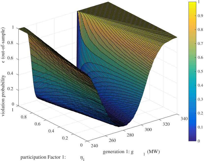
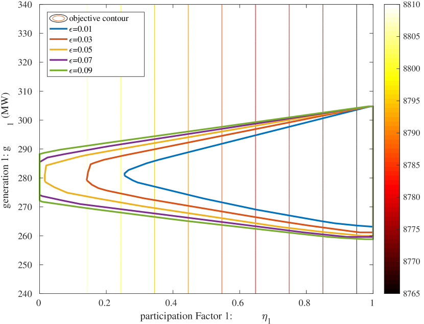
Although there are four variables ($g_{1},g_{2},\eta_{1},\eta_{2}$) in (cc-DCOPF) for the 3-bus system, only two of them (e.g. $g_{1}$ and $\eta_{1}$) are free variables because of constraints (2b) and (2e) . Thanks to this, we could visualize the violation probability function $\mathbb{V}(g_{1},\eta_{1})$ in the 3D space. The function $\mathbb{V}(g_{1},\eta_{1})$ is evaluated over a grid of 65536 points in the $(g_{1},\eta_{1})$ space, the value of $\mathbb{V}(g_{1},\eta_{1})$ at every point is estimated using 1000 i.i.d realizations of uncertainties $\tilde{d}$. Figure 2 shows $\mathbb{V}(g_{1},\eta_{1})$. Based on the estimation of $\mathbb{V}(g_{1},\eta_{1})$, we could also visualize the feasible region $\mathcal{F}_{\epsilon}=\{x:\mathbb{V}(x)\leq\epsilon\}$, which is shown in Figure 3.

Figure 2: Visualization of the Violation Probability Function $\mathbb{V}(x)$ for cc-DCOPF of the 3-bus System

Figure 3: Feasible Region of cc-DCOPF for the 3-bus System (with contours of objective values)

3.3 Simulation Results

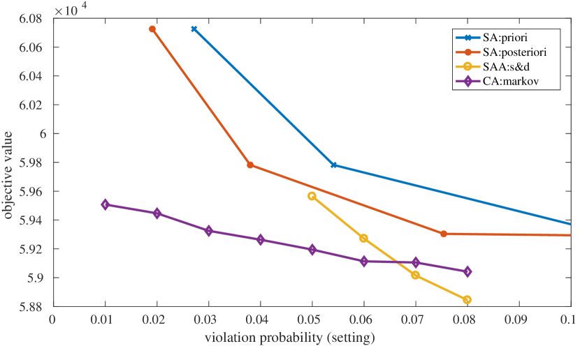
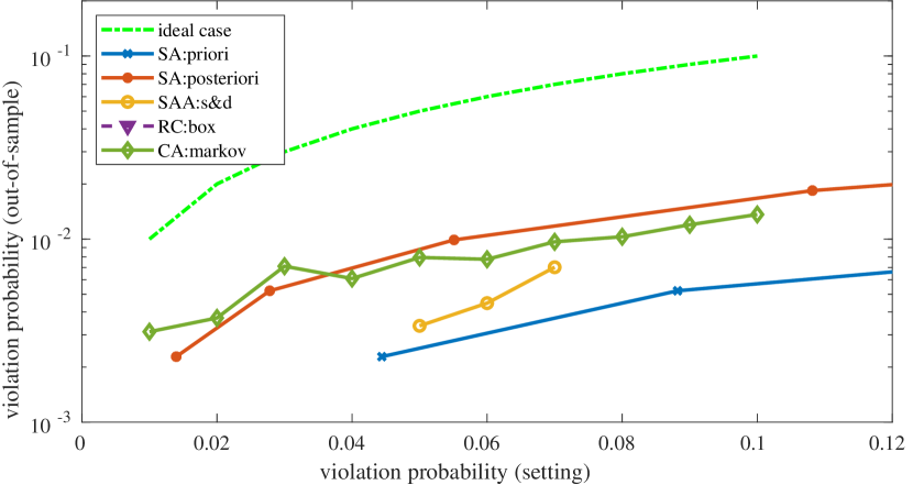
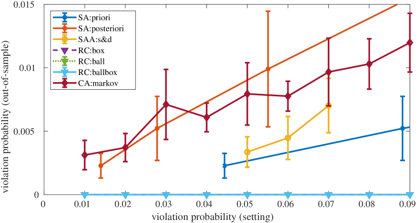
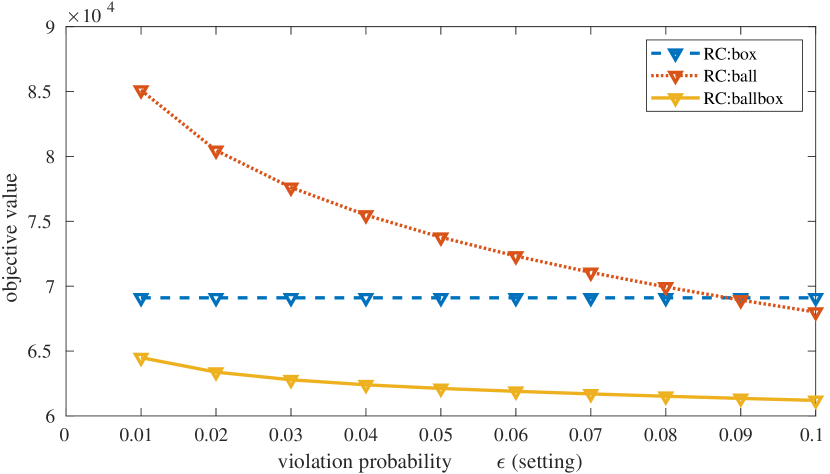
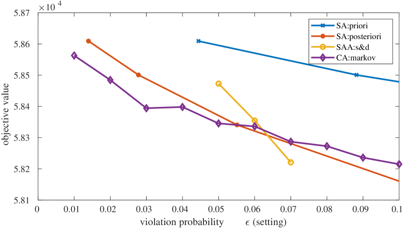
We solve cc-DCOPF on the 3-bus system with eight different methods: (1) scenario approach with prior guarantees, (SA:prior, Corollary LABEL:cor:prior_sample_complexity_fully_supported in (Geng and Xie, 2019a)); (2) scenario approach with posterior guarantees (SA:posterior, Theorem LABEL:thm:posterior_guarantee in (Geng and Xie, 2019a)); (3) sample average approximation, where $N$ and $\varepsilon$ are chosen based on the sampling and discarding Theorem (SAA:s&d, Theorem LABEL:thm:sampling_and_discarding in (Geng and Xie, 2019a)); (4-7) Robust counterpart with different uncertainty sets specified in Theorem LABEL:thm:rlo_safe_approx in (Geng and Xie, 2019a): box (RC:box), ball (RC:ball), ball-box (RC:ball-box) and budget (RC:budget) uncertainty sets; (8) convex approximation with Markov bound (CA:markov, Theorem LABEL:thm:convex_approx_safe_approx and Proposition LABEL:prop:convex_approx_cvar in (Geng and Xie, 2019a)).

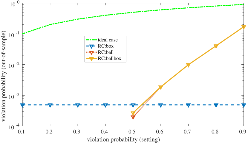
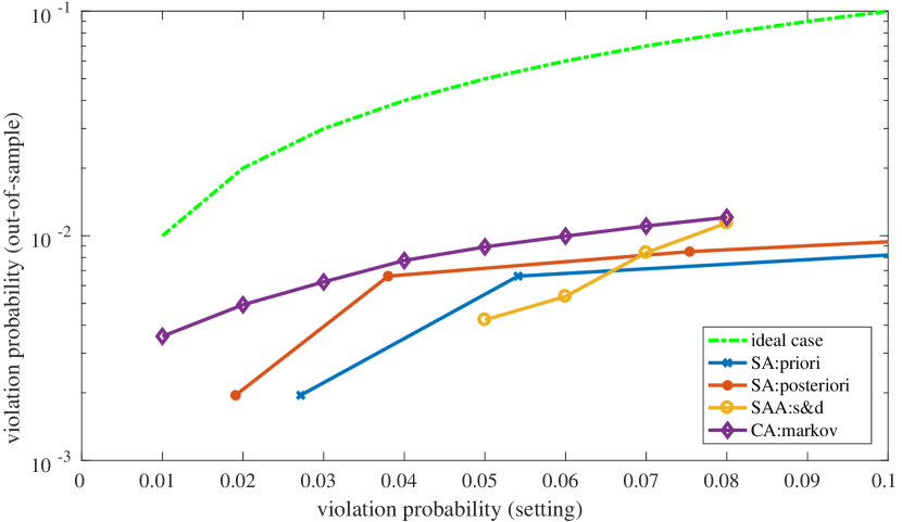
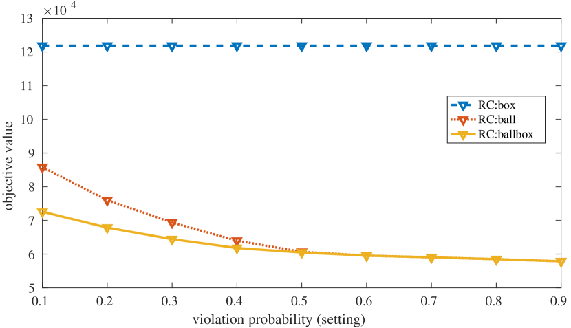
We first examine the feasibility of the returned solutions from eight algorithms. Figure 5 and 6 show the out-of-sample violation probabilities $\hat{\epsilon}$ versus desired $\epsilon$ in the setting. The green dashed lines in Figure 5 and 6 denote the ideal case where $\hat{\epsilon}=\epsilon$. Any points above the green dashed line indicate infeasible solutions that $\mathbb{V}(x)>\epsilon$. Clearly all methods return feasible solutions (with high probability) to (CCO). From Figure 5, sample average approximation and convex approximation are less conservative than other methods. However, it is worth noting that when $\epsilon$ is small (e.g. $10^{-2}$), the data-driven approximation of CVaR (Proposition LABEL:prop:convex_approx_cvar, (Geng and Xie, 2019a)) does not necessarily give a safe approximation to (CCO) (Chen et al., 2010). The robust counterpart methods are typically $10\sim 100$ times more conservative than other methods, as illustrated in the comparison of Figure 6(a) with Figure 6(b). The conservativeness could be significantly reduced by better construction of uncertainty sets, e.g. Chen et al. (2010); Bertsimas et al. (2018). Among four different choices of uncertainty sets, the ball-box set is the least conservative one, which combines the advantages of the ball and box uncertainty sets.

Figure 4: Objective Values (cc-DCOPF of the 3-bus System)

(a) with logarithmic y-axis

(b) with error bars showing standard deviations

Figure 5: Violation Probabilities (cc-DCOPF of the 3-bus System)

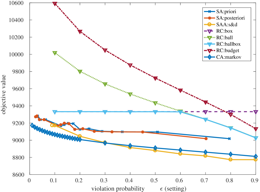
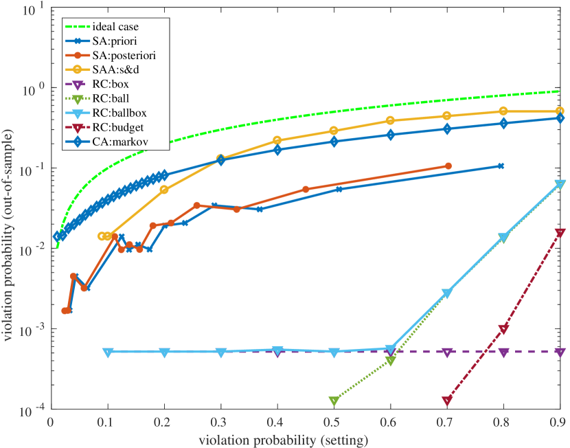
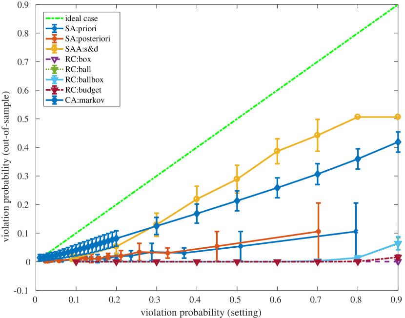
Figure 6-7 present the results of the 24-bus system with Gaussian distributions. Simulation results of the beta distribution are in Figure 8-10. Observations from Figure 8-10 are similar with the case of Gaussian distributions. Every method behaves more conservative in the case of beta distributions than the case of Gaussian distributions. It is worth noting that the RO-based methods (RC:box, RC:ball, RC:ball-box in Figure 9) are so conservative that lead to zero empirical violation probability $\hat{\epsilon}$.

(a) robust counterpart methods

(b) other methods

Figure 6: Violation Probabilities (cc-DCOPF of the 24-bus System, Gaussian Distributions)

(a) robust counterpart methods

(b) other methods

Figure 7: Objective Values (cc-DCOPF of the 24-bus System, Gaussian Distributions)

Figure 8: Violation Probabilities in Logarithmic Scale (cc-DCOPF of the 24-bus System, Beta Distributions)

Figure 9: Violation Probabilities with error bars showing standard deviations (cc-DCOPF of the 24-bus System, Beta Distributions)

(a) robust counterpart methods

(b) other methods

Figure 10: Objective Values (cc-DCOPF of the 24-bus System, Beta Distributions)

4 Concluding Remarks

This paper consists of two parts. The first part presents a comprehensive review on the fundamental properties, key theoretical results, and three classes of algorithms for chance-constrained optimization. An open-source MATLAB toolbox ConvertChanceConstraint is developed to automate the process of translating chance constraints to compatible forms for mainstream optimization solvers. The second part of this paper presents three major applications of chance-constrained optimization in power systems. We also present a critical comparison of existing algorithms to solve chance-constrained programs on IEEE benchmark systems.

Many interesting directions are open for future research. More thorough and detailed comparisons of solutions to (CCO) on various problems with realistic datasets is needed. In terms of theoretical investigation, an analytical comparison of existing solutions to chance-constrained optimization is necessary to substantiate the fundamental insights obtained from numerical simulations. In terms of applications, many existing results can be improved by exploiting the structural properties of the problem to be solved. The application of chance-constrained optimization in electric energy systems could go beyond operational planning practices. For example, it would be worth investigating into the economic interpretation of market power issues through the lens of chance-constrained optimization.

References

- Allan and others (2013) Allan, R.N., others, 2013. Reliability evaluation of power systems. Springer Science & Business Media.
- Bagheri et al. (2017) Bagheri, A., Zhao, C., Guo, Y., 2017. Data-driven chance-constrained stochastic unit commitment under wind power uncertainty, in: Power & Energy Society General Meeting, 2017 IEEE, IEEE. pp. 1–5.
- Bent et al. (2013) Bent, R., Bienstock, D., Chertkov, M., 2013. Synchronization-aware and algorithm-efficient chance constrained optimal power flow, in: Bulk Power System Dynamics and Control-IX Optimization, Security and Control of the Emerging Power Grid (IREP), 2013 IREP Symposium, IEEE. pp. 1–11.
- Bertsimas et al. (2018) Bertsimas, D., Gupta, V., Kallus, N., 2018. Data-driven robust optimization. Mathematical Programming .
- Bertsimas et al. (2013) Bertsimas, D., Litvinov, E., Sun, X.A., Zhao, J., Zheng, T., 2013. Adaptive robust optimization for the security constrained unit commitment problem. IEEE Transactions on Power Systems 28, 52–63.
- Bertsimas and Sim (2004) Bertsimas, D., Sim, M., 2004. The price of robustness. Operations research 52, 35–53.
- Bienstock et al. (2013) Bienstock, D., Chertkov, M., Harnett, S., 2013. Robust modeling of probabilistic uncertainty in smart grids: Data ambiguous chance constrained optimum power flow, in: Decision and Control (CDC), 2013 IEEE 52nd Annual Conference on, IEEE. pp. 4335–4340.
- Bienstock et al. (2014) Bienstock, D., Chertkov, M., Harnett, S., 2014. Chance-constrained optimal power flow: Risk-aware network control under uncertainty. SIAM Review 56, 461–495.
- Bucher et al. (2013) Bucher, M.A., Vrakopoulou, M., Andersson, G., 2013. Probabilistic N- 1 security assessment incorporating dynamic line ratings, in: Power and Energy Society General Meeting (PES), 2013 IEEE, IEEE. pp. 1–5.
- Calafiore and Campi (2005) Calafiore, G., Campi, M.C., 2005. Uncertain convex programs: randomized solutions and confidence levels. Mathematical Programming 102, 25–46.
- Calafiore (2010) Calafiore, G.C., 2010. Random convex programs. SIAM Journal on Optimization 20, 3427–3464.
- Campi and Garatti (2008) Campi, M.C., Garatti, S., 2008. The exact feasibility of randomized solutions of uncertain convex programs. SIAM Journal on Optimization 19, 1211–1230.
- Campi et al. (2018) Campi, M.C., Garatti, S., Ramponi, F.A., 2018. A general scenario theory for non-convex optimization and decision making. IEEE Transactions on Automatic Control .
- Chen et al. (2010) Chen, W., Sim, M., Sun, J., Teo, C.P., 2010. From CVaR to uncertainty set: Implications in joint chance-constrained optimization. Operations research 58, 470–485.
- Ding et al. (2010) Ding, X., Lee, W.J., Jianxue, W., Liu, L., 2010. Studies on stochastic unit commitment formulation with flexible generating units. Electric Power Systems Research 80, 130–141.
- Doostizadeh et al. (2016) Doostizadeh, M., Aminifar, F., Ghasemi, H., Lesani, H., 2016. Energy and reserve scheduling under wind power uncertainty: An adjustable interval approach. IEEE Transactions on Smart Grid 7, 2943–2952.
- Franco et al. (2016) Franco, J.F., Rider, M.J., Romero, R., 2016. Robust multi-stage substation expansion planning considering stochastic demand. IEEE Transactions on Power Systems 31, 2125–2134.
- Geng et al. (2019) Geng, X., Modarresi, S., Xie, L., 2019. Security-constrained Unit Commitment with Probabilistic Guarantees. IEEE Transactions on Power Systems (submitted) .
- Geng and Xie (2019a) Geng, X., Xie, L., 2019a. Data-driven Decision Making with Probabilistic Guarantees (Part 1): A Schematic Overview of Chance-constrained Optimization. arXiv:1903.10621 .
- Geng and Xie (2019b) Geng, X., Xie, L., 2019b. Data-driven Decision Making with Probabilistic Guarantees (Part 2): Applications of Chance-constrained Optimization in Power Systems. arxiv .
- Grigg et al. (1999) Grigg, C., Wong, P., Billinton, R., others, 1999. The IEEE reliability test system-1996. A report prepared by the reliability test system task force of the application of probability methods subcommittee. IEEE Transactions on power systems 14, 1010–1020.
- Gurobi Optimization (2016) Gurobi Optimization, I., 2016. Gurobi Optimizer Reference Manual. URL: http://www.gurobi.com.
- Hodge and Milligan (2011) Hodge, B.M., Milligan, M., 2011. Wind power forecasting error distributions over multiple timescales, in: Power and Energy Society General Meeting, 2011 IEEE, IEEE. pp. 1–8.
- Hreinsson et al. (2015) Hreinsson, K., Vrakopoulou, M., Andersson, G., 2015. Stochastic security constrained unit commitment and non-spinning reserve allocation with performance guarantees. International Journal of Electrical Power & Energy Systems 72, 109–115.
- Jabr (2013) Jabr, R.A., 2013. Adjustable robust OPF with renewable energy sources. IEEE Transactions on Power Systems 28, 4742–4751.
- Jiang et al. (2016) Jiang, R., Guan, Y., Watson, J.P., 2016. Cutting planes for the multistage stochastic unit commitment problem. Mathematical Programming 157, 121–151.
- Jiang et al. (2012) Jiang, R., Wang, J., Guan, Y., 2012. Robust unit commitment with wind power and pumped storage hydro. IEEE Transactions on Power Systems 27, 800.
- Ke et al. (2016) Ke, D., Chung, C., Sun, Y., 2016. A novel probabilistic optimal power flow model with uncertain wind power generation described by customized Gaussian mixture model. IEEE Trans. Sustain. Energy 7, 200–212.
- Lesieutre et al. (2011) Lesieutre, B.C., Molzahn, D.K., Borden, A.R., DeMarco, C.L., 2011. Examining the limits of the application of semidefinite programming to power flow problems, in: Communication, Control, and Computing (Allerton), 2011 49th Annual Allerton Conference on, IEEE. pp. 1492–1499.
- Li and Mathieu (2015) Li, B., Mathieu, J.L., 2015. Analytical reformulation of chance-constrained optimal power flow with uncertain load control, in: PowerTech, 2015 IEEE Eindhoven, IEEE. pp. 1–6.
- Li et al. (2019) Li, B., Vrakopoulou, M., Mathieu, J.L., 2019. Chance Constrained Reserve Scheduling Using Uncertain Controllable Loads Part II: Analytical Reformulation. IEEE Transactions on Smart Grid .
- López et al. (2015) López, J., Pozo, D., Contreras, J., Mantovani, J., 2015. A convex chance-constrained model for reactive power planning. International Journal of Electrical Power & Energy Systems 71, 403–411.
- López et al. (2007) López, J.l., Ponnambalam, K., Quintana, V.H., 2007. Generation and transmission expansion under risk using stochastic programming. IEEE Transactions on Power Systems 22, 1369–1378.
- Lubin et al. (2016) Lubin, M., Dvorkin, Y., Backhaus, S., 2016. A robust approach to chance constrained optimal power flow with renewable generation. IEEE Transactions on Power Systems 31, 3840–3849.
- Manickavasagam et al. (2015) Manickavasagam, M., Anjos, M.F., Rosehart, W.D., 2015. Sensitivity-based chance-constrained generation expansion planning. Electric Power Systems Research 127, 32–40.
- Margellos et al. (2013) Margellos, K., Rostampour, V., Vrakopoulou, M., Prandini, M., Andersson, G., Lygeros, J., 2013. Stochastic unit commitment and reserve scheduling: A tractable formulation with probabilistic certificates, in: Control Conference (ECC), 2013 European, IEEE. pp. 2513–2518.
- Martínez and Anderson (2015) Martínez, G., Anderson, L., 2015. A risk-averse optimization model for unit commitment problems, in: System Sciences (HICSS), 2015 48th Hawaii International Conference on, IEEE. pp. 2577–2585.
- Mazadi et al. (2009) Mazadi, M., Rosehart, W., Malik, O., Aguado, J., 2009. Modified chance-constrained optimization applied to the generation expansion problem. IEEE Transactions on Power Systems 24, 1635–1636.
- Mühlpfordt et al. (2017) Mühlpfordt, T., Faulwasser, T., Roald, L., Hagenmeyer, V., 2017. Solving optimal power flow with non-Gaussian uncertainties via polynomial chaos expansion, in: Decision and Control (CDC), 2017 IEEE 56th Annual Conference on, IEEE. pp. 4490–4496.
- Ming et al. (2017) Ming, H., Xie, L., Campi, M., Garatti, S., Kumar, P., 2017. Scenario-based Economic Dispatch with Uncertain Demand Response. IEEE Transactions on Smart Grid .
- Modarresi et al. (2018) Modarresi, M.S., Xie, L., Campi, M., Garatti, S., Caré, A., Thatte, A., Kumar, P., 2018. Scenario-based Economic Dispatch with Tunable Risk Levels in High-renewable Power Systems. IEEE Transactions on Power Systems .
- Pozo and Contreras (2013) Pozo, D., Contreras, J., 2013. A chance-constrained unit commitment with an $n-k$ security criterion and significant wind generation. IEEE Transactions on Power systems 28, 2842–2851.
- Qiu et al. (2016) Qiu, J., Dong, Z.Y., Zhao, J., Xu, Y., Luo, F., Yang, J., 2016. A risk-based approach to multi-stage probabilistic transmission network planning. IEEE Transactions on Power Systems 31, 4867–4876.
- Roald et al. (2015a) Roald, L., Misra, S., Chertkov, M., Andersson, G., 2015a. Optimal power flow with weighted chance constraints and general policies for generation control, in: Decision and Control (CDC), 2015 IEEE 54th Annual Conference on, IEEE. pp. 6927–6933.
- Roald et al. (2017a) Roald, L., Misra, S., Krause, T., Andersson, G., 2017a. Corrective control to handle forecast uncertainty: A chance constrained optimal power flow. IEEE Transactions on Power Systems 32, 1626–1637.
- Roald et al. (2017b) Roald, L., Misra, S., Morrison, A., Andersson, G., 2017b. Optimized risk limits for stochastic optimal power flow, in: Decision and Control (CDC), 2017 IEEE 56th Annual Conference on, IEEE. pp. 4476–4483.
- Roald et al. (2013) Roald, L., Oldewurtel, F., Krause, T., Andersson, G., 2013. Analytical reformulation of security constrained optimal power flow with probabilistic constraints, in: PowerTech (POWERTECH), 2013 IEEE Grenoble, IEEE. pp. 1–6.
- Roald et al. (2014) Roald, L., Vrakopoulou, M., Oldewurtel, F., Andersson, G., 2014. Risk-constrained optimal power flow with probabilistic guarantees, in: Power Systems Computation Conference (PSCC), 2014, IEEE. pp. 1–7.
- Roald et al. (2015b) Roald, L., Vrakopoulou, M., Oldewurtel, F., Andersson, G., 2015b. Risk-based optimal power flow with probabilistic guarantees. International Journal of Electrical Power & Energy Systems 72, 66–74.
- Sanghvi et al. (1982) Sanghvi, A.P., Shavel, I.H., Spann, R.M., 1982. Strategic planning for power system reliability and vulnerability: an optimization model for resource planning under uncertainty. IEEE Transactions on Power Apparatus and Systems , 1420–1429.
- Summers et al. (2014) Summers, T., Warrington, J., Morari, M., Lygeros, J., 2014. Stochastic optimal power flow based on convex approximations of chance constraints, in: Power Systems Computation Conference (PSCC), IEEE.
- Summers et al. (2015) Summers, T., Warrington, J., Morari, M., Lygeros, J., 2015. Stochastic optimal power flow based on conditional value at risk and distributional robustness. International Journal of Electrical Power & Energy Systems 72, 116–125.
- Takriti et al. (1996) Takriti, S., Birge, J.R., Long, E., 1996. A stochastic model for the unit commitment problem. IEEE Transactions on Power Systems 11, 1497–1508.
- Tan and Shaaban (2016) Tan, W.S., Shaaban, M., 2016. A hybrid stochastic/deterministic unit commitment based on projected disjunctive milp reformulation. IEEE Transactions on Power Systems 31, 5200–5201.
- Vrakopoulou et al. (2019) Vrakopoulou, M., Li, B., Mathieu, J.L., 2019. Chance Constrained Reserve Scheduling Using Uncertain Controllable Loads Part I: Formulation and Scenario-based Analysis. IEEE Transactions on Smart Grid .
- Vrakopoulou et al. (2013a) Vrakopoulou, M., Margellos, K., Lygeros, J., Andersson, G., 2013a. A probabilistic framework for reserve scheduling and security assessment of systems with high wind power penetration. IEEE Transactions on Power Systems 28, 3885–3896.
- Vrakopoulou et al. (2013b) Vrakopoulou, M., Margellos, K., Lygeros, J., Andersson, G., 2013b. Probabilistic guarantees for the N-1 security of systems with wind power generation, in: Reliability and Risk Evaluation of Wind Integrated Power Systems. Springer, pp. 59–73.
- Wang et al. (2012) Wang, Q., Guan, Y., Wang, J., 2012. A chance-constrained two-stage stochastic program for unit commitment with uncertain wind power output. IEEE Transactions on Power Systems 27, 206–215.
- Wang et al. (2013) Wang, Q., Wang, J., Guan, Y., 2013. Price-based unit commitment with wind power utilization constraints. IEEE Transactions on Power Systems 28, 2718–2726.
- Wang et al. (2017) Wang, Z., Shen, C., Liu, F., Wu, X., Liu, C.C., Gao, F., 2017. Chance-constrained economic dispatch with non-Gaussian correlated wind power uncertainty. IEEE Transactions on Power Systems 32, 4880–4893.
- Wu et al. (2014) Wu, H., Shahidehpour, M., Li, Z., Tian, W., 2014. Chance-constrained day-ahead scheduling in stochastic power system operation. IEEE Transactions on Power Systems 29, 1583–1591.
- Wu et al. (2007) Wu, L., Shahidehpour, M., Li, T., 2007. Stochastic Security-Constrained Unit Commitment. IEEE Transactions on Power Systems 22, 800–811. doi:10.1109/TPWRS.2007.894843.
- Wu et al. (2016) Wu, Z., Zeng, P., Zhang, X.P., Zhou, Q., 2016. A solution to the chance-constrained two-stage stochastic program for unit commitment with wind energy integration. IEEE Transactions on Power Systems 31, 4185–4196.
- Xie et al. (2011) Xie, L., Carvalho, P.M., Ferreira, L.A., Liu, J., Krogh, B.H., Popli, N., Ilic, M.D., 2011. Wind integration in power systems: Operational challenges and possible solutions. Proceedings of the IEEE 99, 214–232.
- Yang and Wen (2005) Yang, N., Wen, F., 2005. A chance constrained programming approach to transmission system expansion planning. Electric Power Systems Research 75, 171–177.
- Yang and Nehorai (2014) Yang, P., Nehorai, A., 2014. Joint optimization of hybrid energy storage and generation capacity with renewable energy. IEEE Transactions on Smart Grid 5, 1566–1574.
- Zhang and Giannakis (2013) Zhang, Y., Giannakis, G.B., 2013. Robust optimal power flow with wind integration using conditional value-at-risk, in: Smart Grid Communications (SmartGridComm), 2013 IEEE International Conference on, IEEE. pp. 654–659.
- Zhang et al. (2017a) Zhang, Y., Shen, S., Mathieu, J., 2017a. Distributionally Robust Chance-Constrained Optimal Power Flow with Uncertain Renewables and Uncertain Reserves Provided by Loads. IEEE Transactions on Power Systems .
- Zhang et al. (2015) Zhang, Y., Shen, S., Mathieu, J.L., 2015. Data-driven optimization approaches for optimal power flow with uncertain reserves from load control, in: American Control Conference (ACC), 2015, IEEE. pp. 3013–3018.
- Zhang et al. (2017b) Zhang, Y., Wang, J., Li, Y., Cao, X., 2017b. Chance-constrained Transmission Expansion Planning with Guaranteed Wind Power Utilization, Chicago, IL.
- Zhang et al. (2017c) Zhang, Y., Wang, J., Zeng, B., Hu, Z., 2017c. Chance-Constrained Two-Stage Unit Commitment under Uncertain Load and Wind Power Output Using Bilinear Benders Decomposition. IEEE Trans on Power Systems .
- Zhao et al. (2014) Zhao, C., Wang, Q., Wang, J., Guan, Y., 2014. Expected value and chance constrained stochastic unit commitment ensuring wind power utilization. IEEE Transactions on Power Systems 29, 2696–2705.
- Zheng et al. (2015) Zheng, Q.P., Wang, J., Liu, A.L., 2015. Stochastic optimization for unit commitment—A review. IEEE Trans. Power Syst 30, 1913–1924.
- Zimmerman et al. (2011) Zimmerman, R.D., Murillo-Sánchez, C.E., Thomas, R.J., 2011. MATPOWER: Steady-state operations, planning, and analysis tools for power systems research and education. IEEE Transactions on power systems 26, 12–19.