NuPhys2018-King

Theory Review of Neutrino Models and CP Violation

Stephen F King

Department of Physics and Astronomy
University of Southampton, Southampton, SO17 1BJ, U.K.

Although the measurement of the reactor angle has killed tribimaximal lepton mixing, its descendants survive with charged lepton corrections, or in less constrained forms such as trimaximal mixing and/or mu-tau symmetry, each with characteristic predictions. Such patterns may be enforced by a remnant of some non-Abelian discrete family symmetry, possibly together with a generalised CP symmetry, which could originate from continuous gauge symmetry and/or superstring theory in compactified extra dimensions, as a finite subgroup of the modular symmetry.

PRESENTED AT

NuPhys2018, Prospects in Neutrino Physics,
Cavendish Conference Centre,
London, UK, December 19–21, 2018

1 Introduction

Neutrino physics has made remarkable progress since the discovery of neutrino mass and mixing in 1998 [1]. The reactor angle, unknown before 2012, is now accurately measured by Daya Bay: $\theta_{13}\approx 8.5^{\circ}\pm 0.2^{\circ}$ [2]. The other lepton mixing angles are determined from global fits to be in the three sigma ranges: $\theta_{12}\approx 32-36^{\circ}$ and $\theta_{23}\approx 40-52^{\circ}$, with the first hints of the CP-violating (CPV) phase $\delta=125-390^{\circ}$. The best global fit values with one sigma errors are given in Table 2 [3] where the meaning of the angles is given in Table 2.

	NuFIT 4.0
$\theta_{12}$ [∘]	$33.82^{+0.78\phantom{0}}_{-0.76}$
$\theta_{13}$ [∘]	$8.61^{+0.13\phantom{0}}_{-0.13}$
$\theta_{23}$ [∘]	$49.6^{+1.0\phantom{00}}_{-1.2}$
$\delta$ [∘]	$-145^{+40\phantom{.00}}_{-29}$
$\Delta m^{2}_{21}$ [$10^{-5}\rm{eV}^{2}$]	$7.39^{+0.21\phantom{0}}_{-0.20}$
$\Delta m^{2}_{31}$ [$10^{-3}\rm{eV}^{2}$]	$2.525^{+0.033}_{-0.032}$

Table 1: The nu-fit 4.0 results with one sigma errors without SK atmospheric data for the normal ordered (NO) case, favoured by current data [3].

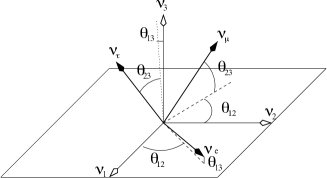
Table 2: Neutrino mixing angles may be represented as Euler angles relating the states in the charged lepton mass basis $(\nu_{e},\nu_{\mu},\nu_{\tau})$ to the mass eigenstate basis states $(\nu_{1},\nu_{2},\nu_{3})$.

The measurement of the reactor angle had a major impact on models of neutrino mass and mixing as reviewed in [4, 5, 6] (for earlier reviews see e.g. [7, 8, 9]). In this talk we give a brief theoretical overview of current neutrino models and CP violation.

2 Quark vs Lepton Mixing

The CKM and PMNS mixing matrices are (in the PDG parametrisation):

$$\!\!\!\!\!\!\!\!\!\!\!\!\!\!\!\!\!\left(\begin{array}[]{ccc}c_{12}c_{13}&s_{12}c_{13}&s_{13}e^{-i\delta}\\ -s_{12}c_{23}-c_{12}s_{13}s_{23}e^{i\delta}&\hphantom{+}c_{12}c_{23}-s_{12}s_{13}s_{23}e^{i\delta}&c_{13}s_{23}\\ \hphantom{+}s_{12}s_{23}-c_{12}s_{13}c_{23}e^{i\delta}&-c_{12}s_{23}-s_{12}s_{13}c_{23}e^{i\delta}&c_{13}c_{23}\end{array}\right)$$ (4)

where $s_{13}=\sin\theta_{13}$, etc. with (very) different angles for quarks and leptons. In the case of Majorana neutrinos, the PMNS matrix also involves the Majorana phase matrix: $P_{M}=\textrm{diag}(1,e^{i\frac{\alpha_{21}}{2}},e^{i\frac{\alpha_{31}}{2}})$ which post-multiplies the above matrix.

It is interesting to compare quark mixing, which is small,

$$s^{q}_{12}=\lambda,\ \ s^{q}_{23}\sim\lambda^{2},\ \ s^{q}_{13}\sim\lambda^{3}$$ (5)

where the Wolfenstein parameter is $\lambda=0.226\pm 0.001$, to lepton mixing, which is large,

$$s_{13}\sim\lambda/\sqrt{2},\ \ s_{23}\sim 1/\sqrt{2},\ \ s_{12}\sim 1/\sqrt{3}.$$ (6)

The smallest lepton mixing angle $\theta_{13}$ (the reactor angle), is of order the largest quark mixing angle $\theta^{q}_{12}=\theta_{C}=13.0^{\circ}$ (the Cabibbo angle, where $\sin\theta_{C}=\lambda$). There have been attempts to relate quark and lepton mixing angles such as postulating a reactor angle $\theta_{13}=\theta_{C}/\sqrt{2}$ [10], and the CP violating lepton phase $\delta\sim-\pi/2$ (c.f. the well measured CP violating quark phase $\delta^{q}\sim(\pi/2)/\sqrt{2}$).

3 Tribimaximal mixing and its descendants

The tribimaximal (TB) mixing matrix [11] postulated zero reactor angle $s^{2}_{13}=\theta_{13}=0$ (hence zero Dirac CP violation), maximal atmospheric angle $s^{2}_{23}=1/2$ ($\theta_{23}=45^{\circ}$) and a solar mixing angle given by $s_{12}=1/\sqrt{3}$ ($\theta_{12}\approx 35.26^{\circ}$). The mixing matrix is given explicitly by

$$U_{\rm TB}=\left(\begin{array}[]{ccc}\sqrt{\frac{2}{3}}&\frac{1}{\sqrt{3}}&0\\ -\frac{1}{\sqrt{6}}&\frac{1}{\sqrt{3}}&\frac{1}{\sqrt{2}}\\ \frac{1}{\sqrt{6}}&-\frac{1}{\sqrt{3}}&\frac{1}{\sqrt{2}}\end{array}\right)P_{M},$$ (7)

where $P_{M}$ is the Majorana phase matrix defined above (frequently ignored). The trimaximal symmetry of the second column, and bimaximal symmetry of the second and third rows, motivates the use of non-Abelian discrete symmetries such as A₄ [12]. TB mixing was killed  by the measurement of the reactor angle, but it has surviving descendants as follows.

3.1 Trimaximal lepton mixing and atmospheric sum rules

The first surviving descendants of TB mixing are the twins known as trimaximal $\rm{TM}_{1}$ or $\rm{TM}_{2}$ lepton mixing which preserve the first or the second column of Eq.7 [13],

$$\!\!\!\!\!\!\!\!|U_{\rm TM_{1}}|=\left(\begin{array}[]{ccc}\frac{2}{\sqrt{6}}&-&-\\ \frac{1}{\sqrt{6}}&-&-\\ \frac{1}{\sqrt{6}}&-&-\end{array}\right),\ \ \ \ |U_{\rm TM_{2}}|=\left(\begin{array}[]{ccc}-&\frac{1}{\sqrt{3}}&-\\ -&\frac{1}{\sqrt{3}}&-\\ -&\frac{1}{\sqrt{3}}&-\end{array}\right).$$ (8)

These forms survive since the reactor angle becomes a free parameter, while the solar angle may remains close to its TB prediction (in agreement with data). The unfilled entries are fixed when the reactor angle is specified. It is important to emphasise that these forms are more than simple ansatze, since they may be enforced by discrete non-Abelian family symmetry, as discussed in section 4. For example, $\rm{TM}_{2}$ mixing can be realised by $A_{4}$ or $S_{4}$ symmetry [14], while $\rm{TM}_{1}$ mixing can be realised by $S_{4}$ symmetry [15]. A general group theory analysis of semi-direct symmetries was given in [16].

$\rm{TM}_{1}$ implies three equivalent relations:

$$\tan\theta_{12}=\frac{1}{\sqrt{2}}\sqrt{1-3s^{2}_{13}}\ \ \ \ {\rm or}\ \ \ \ \sin\theta_{12}=\frac{1}{\sqrt{3}}\frac{\sqrt{1-3s^{2}_{13}}}{c_{13}}\ \ \ \ {\rm or}\ \ \ \ \cos\theta_{12}=\sqrt{\frac{2}{3}}\frac{1}{c_{13}}$$ (9)

leading to a prediction $\theta_{12}\approx 34^{\circ}$, in excellent agreement with current global fits, assuming $\theta_{13}\approx 8.5^{\circ}$. By contrast, the corresponding $\rm{TM}_{2}$ relations imply $\theta_{12}\approx 36^{\circ}$ [13], which is on the edge of the three sigma region, and hence disfavoured by current data. $\rm{TM}_{1}$ mixing also leads to an exact sum rule relation relation for $\cos\delta$ in terms of the other lepton mixing angles [13],

$$\cos\delta=-\frac{\cot 2\theta_{23}(1-5s^{2}_{13})}{2\sqrt{2}s_{13}\sqrt{1-3s^{2}_{13}}},$$ (10)

which, for approximately maximal atmospheric mixing, predicts $\cos\delta\approx 0$, $\delta\approx\pm 90^{\circ}$.  Such atmospheric mixing sum rules may be tested in future experiments [17].

For example, the Littlest Seesaw (LS) model [18] leads to $\rm{TM}_{1}$ mixing, for two cases of light Majorana neutrino mass matrix (in the diagonal charged lepton basis):

$$\rm{Case\ I:}\ \ \ \ M^{I}_{\nu}=\omega m_{a}\left(\begin{array}[]{ccc}0&0&0\\ 0&1&1\\ 0&1&1\end{array}\right)+m_{s}\left(\begin{array}[]{ccc}1&3&1\\ 3&9&3\\ 1&3&1\end{array}\right)$$ (11)

$$\rm{Case\ II:}\ \ \ \ M^{II}_{\nu}=\omega^{2}m_{a}\left(\begin{array}[]{ccc}0&0&0\\ 0&1&1\\ 0&1&1\end{array}\right)+m_{s}\left(\begin{array}[]{ccc}1&1&3\\ 1&1&3\\ 3&3&9\end{array}\right)$$ (12)

where $\omega=e^{i2\pi/3}$. The LS is very predictive since there are only two free (real) input parameters, where $m_{a}\approx 26$ meV and $m_{s}\approx 2.6$ meV gives the best fit to neutrino masses with $m_{1}=0$ and PMNS parameters including $\theta_{23}\approx 45^{\circ}$, $\delta\approx-90^{\circ}$ (the latter two predictions explained by an approximate mu-tau symmetry as discussed later).

3.2 Charged lepton mixing corrections and solar sum rules

The second way that TB neutrino mixing can survive is due to charged lepton corrections. Recall that the physical PMNS matrix in Eq.4 is given by $U_{\rm PMNS}=U^{e}U^{\nu}$. Now suppose that $U^{\nu}=U^{\nu}_{\rm TB}$, the TB matrix in Eq.7, while $U^{e}$ corresponds to small but unknown charged lepton corrections. This was first discussed in [19, 20, 21, 22] where the following sum rule involving the lepton mixing parameters, including crucially the CP phase $\delta$, was first derived (where $35.26^{o}=\sin^{-1}\frac{1}{\sqrt{3}}$):

$$\!\!\!\!\!\!\!\!\!\!\theta_{12}\approx 35.26^{o}+\theta_{13}\cos\delta,$$ (13)

To derive this sum rule, let us consider the case of the charged lepton mixing corrections involving only (1,2) mixing, so that the PMNS matrix is given by [22],

$$\!U_{\mathrm{PMNS}}=\left(\begin{array}[]{ccc}\!c^{e}_{12}&s^{e}_{12}e^{-i\delta^{e}_{12}}&0\!\\ \!-s^{e}_{12}e^{i\delta^{e}_{12}}&c^{e}_{12}&0\!\\ \!0&0&1\!\end{array}\right)\left(\begin{array}[]{ccc}\sqrt{\frac{2}{3}}&\frac{1}{\sqrt{3}}&0\\ -\frac{1}{\sqrt{6}}&\frac{1}{\sqrt{3}}&\frac{1}{\sqrt{2}}\\ \frac{1}{\sqrt{6}}&-\frac{1}{\sqrt{3}}&\frac{1}{\sqrt{2}}\end{array}\right)=\left(\begin{array}[]{ccc}\!\cdots&\ \ \!\cdots&\!\frac{s^{e}_{12}}{\sqrt{2}}e^{-i\delta^{e}_{12}}\\ \!\cdots&\ \ \!\cdots&\!\frac{c^{e}_{12}}{\sqrt{2}}\!\\ \frac{1}{\sqrt{6}}&-\frac{1}{\sqrt{3}}&\frac{1}{\sqrt{2}}\end{array}\right)$$ (14)

Comparing Eq. 14 to the PMNS parametrisation in Eq.4, we identify the exact sum rule relations [22], in terms of the elements $|U_{e3}|,|U_{\tau 1}|,|U_{\tau 2}|,|U_{\tau 3}|$ identified above. The first element $|U_{e3}|=\frac{s^{e}_{12}}{\sqrt{2}}$ implies a reactor angle $\theta_{13}\approx 9^{\circ}$ if $\theta_{e}\approx\theta_{C}$ (see e.g. the models in [10]). The second and third elements, $|U_{\tau 1}|,|U_{\tau 2}|$ after eliminating $\theta_{23}$, yield a new relation between the PMNS parameters, $\theta_{12}$, $\theta_{13}$ and $\delta$. Expanding to first order gives the approximate solar sum rule relations in Eq.13 [19]. The fourth element implies $s_{23}^{2}<1/2$ which is somewhat disfavoured by global fits.

The above derivation assumes only $\theta^{e}_{12}$ charged lepton corrections. However it is possible to derive an accurate sum rule which is valid for both $\theta^{e}_{12}$ and $\theta^{e}_{23}$ charged lepton corrections (while keeping $\theta^{e}_{13}=0$). Indeed, using a similar matrix multiplication method to that employed above leads to the exact result [23]:

$$\frac{\left|U_{\tau 1}\right|}{\left|U_{\tau 2}\right|}=\frac{|s_{12}s_{23}-c_{12}s_{13}c_{23}e^{i\delta}|}{|-c_{12}s_{23}-s_{12}s_{13}c_{23}e^{i\delta}|}=\frac{1}{\sqrt{2}}\;.$$ (15)

After some algebra, Eq.15 leads to [23],

$$\cos\delta=\frac{t_{23}s^{2}_{12}+s^{2}_{13}c^{2}_{12}/t_{23}-\frac{1}{3}(t_{23}+s^{2}_{13}/t_{23})}{\sin 2\theta_{12}s_{13}}.$$ (16)

To leading order in $\theta_{13}$, Eq.16 returns the sum rule in Eq.13, from which we find $\cos\delta\approx 0$ if $\theta_{12}\approx 35^{o}$, consistent with $\delta\approx-\pi/2$. This can also be understood directly from Eq.16 where we see that for $s_{12}^{2}=1/3$ the leading terms $t_{23}s^{2}_{12}$ and $\frac{1}{3}t_{23}$ cancel in the numerator, giving $\cos\delta=s_{13}/(2\sqrt{2}t_{23})\approx 0.05$ to be compared to $\cos\delta\approx 0$ in the linear approximation. In general the error induced by using the linear sum rule instead of the exact one has been shown to be $\Delta(\cos\delta)<0.1$ [23] for the TB sum rule. Recently there has been much activity in exploring the phenomenology of various such solar mixing sum rules [24]. On the other hand, for a GUT example with $\theta^{e}_{12}\sim\theta_{C}/3$ and $\theta^{e}_{13}\sim\theta_{C}$ which violates the solar mixing sum rules see [25].

4 Family Symmetry Models

The original motivation for family symmetry was to derive or enforce the TB mixing pattern, or one of the other simple patterns such as BM or GR. These days, the motivation is similar, but applied to one of the surviving descendants of TB mixing.

4.1 Symmetry of the mass matrices

The starting point for family symmetry models is to consider the symmetry of the mass matrices. In a basis where the charged lepton mass matrix $M_{e}$ is diagonal, the symmetry is,

$$T^{\dagger}(M_{e}^{\dagger}M_{e})T=M_{e}^{\dagger}M_{e}$$ (17)

where $T={\rm diag}(1,\omega^{2},\omega)$ and $\omega=e^{i2\pi/n}$. For example for $n=3$ clearly $T$ generates the group $Z^{T}_{3}$. The Klein symmetry $Z^{S}_{2}\times Z^{U}_{2}$ of the light Majorana neutrino mass matrix is given by [4],

$$M^{\nu}=S^{T}M^{\nu}S,\ \ \ \ M^{\nu}=U^{T}M^{\nu}U$$ (18)

$$S=U_{\rm PMNS}^{*}\ {\rm diag}(+1,-1,-1)\ U_{\rm PMNS}^{T}$$ (19)

$$U=U_{\rm PMNS}^{*}\ {\rm diag}(-1,+1,-1)\ U_{\rm PMNS}^{T}.$$ (20)

4.2 Direct Models

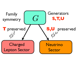
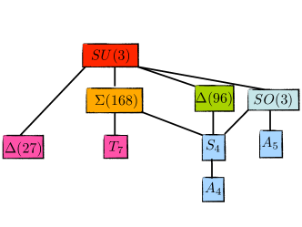
Figure 1: The diagram on the left illustrates the so called direct approach to models of lepton mixing. The diagram on the right shows possible choices of the group $G$.

The idea of “direct models” [4], illustrated in Fig. 1 (left panel), is that the three generators $S,T,U$ introduced above are embedded into a discrete family symmetry $G$ which is broken by new Higgs fields called “flavons” of two types: $\phi^{l}$ whose VEVs preserve $T$ and $\phi^{\nu}$ whose VEVs preserve $S,U$. These flavons are segregated such that $\phi^{l}$ only appears in the charged lepton sector and $\phi^{\nu}$ only appears in the neutrino sector, thereby enforcing the symmetries of the mass matrices. Note that the full Klein symmetry $Z^{S}_{2}\times Z^{U}_{2}$ of the neutrino mass matrix is enforced by symmetry in the direct approach.

There are many choices of the group $G$, with some examples given in Fig. 1 (right panel), with each choice leading to different lepton mixing being predicted. For example, consider the group $S_{4}$ whose irreducible triplet representations are:  

$$\!\!\!\!\!\!\!\!\!\!\!\!\!\!\!\!\!S=\frac{1}{3}\left(\begin{array}[]{ccc}-1&2&2\\ 2&-1&2\\ 2&2&-1\end{array}\right),\ \ \ \ T=\left(\begin{array}[]{ccc}1&0&0\\ 0&\omega^{2}&0\\ 0&0&\omega\end{array}\right),\ \ \ \ U=\mp\left(\begin{array}[]{ccc}1&0&0\\ 0&0&1\\ 0&1&0\end{array}\right)$$ (30)

where $\omega=e^{i2\pi/3}$. Assuming these $S_{4}$ matrices, the $Z^{T}_{3}$ symmetry of the charged lepton mass matrix and the Klein symmetry $Z^{S}_{2}\times Z^{U}_{2}$ of the neutrino mass matrix leads to the prediction of TB mixing (indeed one can check that $S$ and $U$ are diagonalised by $U_{TB}$ as in Eqs.19,20).

4.3 Semi-direct and tri-direct CP models

In the “semi-direct” approach [4], in order to obtain a non-zero reactor angle, one of the generators $T$ or $U$ of the residual symmetry is assumed to be broken. For example, consider the following two interesting possibilities:

1. The $Z_{3}^{T}$ symmetry of the charged lepton mass matrix is broken, but the full Klein symmetry $Z_{2}^{S}\times Z_{2}^{U}$ in the neutrino sector is respected. This corresponds to having charged lepton corrections, with solar sum rules in section 3.2.

2. The $Z_{2}^{U}$ symmetry of the neutrino mass matrix is broken, but the $Z_{3}^{T}$ symmetry of the charged lepton mass matrix is unbroken. In addition either $Z_{2}^{S}$ or $Z_{2}^{SU}$ (with $SU$ being the product of $S$ and $U$) is preserved. This leads to either $\rm{TM}_{1}$ mixing (if $Z_{2}^{SU}$ is preserved [15]); or $\rm{TM}_{2}$ mixing (if $Z_{2}^{S}$ is preserved [14]). Then we have the atmospheric sum rules as discussed in section 3.1.

The “semi-direct approach” may be extended to include a generalised CP symmetry $X$ such that $(M^{\nu})^{*}=X^{T}M^{\nu}X$, with a separate flavour and CP symmetry in the neutrino and charged lepton sectors [26] (see also [27]). Such models typically tend to predict maximal CP violation $\delta=\pm\pi/2$ (the first example of such generalised CP symmetry is mu-tau reflection symmetry discussed in the following subsection).

In the “tri-direct” CP approach [28], a separate flavour and CP symmetry is assumed for each right-handed neutrino sector (in the framework of two right-handed neutrino models [29]) in addition to the charged lepton sector.

4.4 Mu-tau reflection symmetry

An early class of flavour CP models are based on mu-tau reflection symmetry under which $\nu_{\mu}\leftrightarrow\nu_{\tau}^{*}$ (where the star indicates CP conjugation) leading to the prediction of maximal atmospheric mixing $\theta_{23}=\pi/4$ and maximal CP violation $\delta=\pm\pi/2$ [30]. This implies that the elements of the second and third rows of the PMNS matrix $U_{PMNS}$ are related by complex conjugation [30] and have equal magnitudes [31]; and that the elements of the light Majorana neutrino mass matrix $M^{\nu}$ are related [32].

For example, the following $\mu\tau$-LS light Majorana neutrino mass matrices [33]

$$M^{I}_{\nu}=m_{s}\left(\begin{array}[]{ccc}1&3&1\\ 3&9+11\omega&3+11\omega\\ 1&3+11\omega&1+11\omega\\ \end{array}\right),\ \ \ \ M^{II}_{\nu}=m_{s}\left(\begin{array}[]{ccc}1&1&3\\ 1&1+11\omega^{2}&3+11\omega^{2}\\ 3&3+11\omega^{2}&9+11\omega^{2}\\ \end{array}\right)\,$$ (37)

where $\omega=e^{i2\pi/3}$, both lead to the PMNS matrix

$$U^{LS}_{\mu\tau}=\left(\begin{array}[]{ccc}\frac{2}{\sqrt{6}}&\frac{c_{+}}{\sqrt{6}}&\frac{c_{-}}{\sqrt{6}}\\ \frac{1}{\sqrt{6}}&-\frac{c_{+}}{\sqrt{6}}-i\frac{c_{-}}{2}&-\frac{c_{-}}{\sqrt{6}}+i\frac{c_{+}}{2}\\ \frac{1}{\sqrt{6}}&-\frac{c_{+}}{\sqrt{6}}+i\frac{c_{-}}{2}&-\frac{c_{-}}{\sqrt{6}}-i\frac{c_{+}}{2}\\ \end{array}\right)$$ (41)

which clearly respects $\mu-\tau$ reflection symmetry and is a special case of tri-maximal TM₁ mixing [13] in Eq.8, with a fixed reactor angle $\frac{c_{-}}{\sqrt{6}}$, where $c_{\pm}=\sqrt{1\pm\frac{11}{3\sqrt{17}}}$. We emphasise that the neutrino mass matrices in Eq.37 have only one free parameter, namely the neutrino mass scale $m_{s}$ and so are highly (maximally) predictive! Remarkably, the predicted neutrino masses and PMNS parameters can agree with data after including renormalisation group running effects [33].

5 Origin of the non-Abelian discrete symmetry

While early family symmetry models focussed on continuous non-Abelian gauge theories such as $SO(3)$ [19] or $SU(3)$ [34], non-Abelian discrete symmetries [9] are more closely related to TB mixing or its descendants. Here we briefly mention two possible origins of such symmetry.

5.1 Discrete symmetry from continuous symmetry

It is possible to obtain a non-Abelian discrete symmetry starting from a continuous one [35]. For example, we have discussed [36] the breaking of supersymmetric $SO(3)$ gauge theory down to $A_{4}$, where the $A_{4}$ may be subsequently broken to smaller residual symmetries $Z_{3}$ and $Z_{2}$, which may be used to govern the mixing patterns in the charged lepton and neutrino sectors. The basic idea is to use a flavon in the $7$ dimensional representation of $SO(3)$ aligned in a particular direction to break it to $A_{4}$, as depicted in Tables 4,4. Further details are given in [36].

Table 3: Subgroups of $SO(3)$ preserved when it is broken by flavons in the $1,3,5,7$ dimensional representations of $SO(3)$.

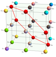
Table 4: $A_{4}$ preserving direction of the $7$ dimensional representations of $SO(3)$ (depicted by the red spheres).

5.2 Discrete symmetry from extra dimensions

Non-Abelian discrete symmetries may arise from superstring theory in compactified extra dimensions, as a finite subgroup of modular symmetry in the target space [37, 38, 39, 40, 41]. Consider a theory with two extra dimensions $x=x_{5}$ and $y=x_{6}$ compactified on a torus $T^{2}$. If the torus is cut open, its surface is a flat rectangle. Allowing for a twist angle $\theta$, the torus surface becomes a parallelogram, and an infinite tiling of such parallelograms with identified sides fills the $(x,y)$ (or complex $z=x+iy$) plane to form a lattice structure as shown in Fig. 2.

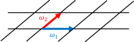
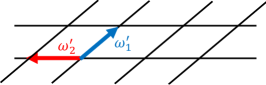
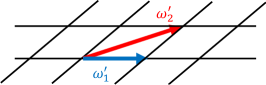
Figure 2: Two extra dimensions compactified on a torus with a twist angle $\theta$ can be represented by a lattice in the complex plane, with basis vectors as shown.

The lattice is described by two basis vectors $(\omega_{1},\omega_{2})$ in the complex $z$ plane, as shown in the first panel of Fig. 2. However the choice of lattice basis vectors is not unique, and different choices of basis vectors $(\omega^{\prime}_{1},\omega^{\prime}_{2})$ can describe the same lattice. There are two independent transformations on the basis vectors $(\omega_{1},\omega_{2})$ which leave the lattice invariant as follows.

The $S$ transformation:

$$\left(\begin{array}[]{c}\omega^{\prime}_{1}\\ \omega^{\prime}_{2}\\ \end{array}\right)=\left(\begin{array}[]{cc}0&1\\ -1&0\\ \end{array}\right)\left(\begin{array}[]{c}\omega_{1}\\ \omega_{2}\\ \end{array}\right)=\left(\begin{array}[]{c}\omega_{2}\\ -\omega_{1}\\ \end{array}\right)$$ (50)

and the $T$ transformation:

$$\left(\begin{array}[]{c}\omega^{\prime}_{1}\\ \omega^{\prime}_{2}\\ \end{array}\right)=\left(\begin{array}[]{cc}1&0\\ 1&1\\ \end{array}\right)\left(\begin{array}[]{c}\omega_{1}\\ \omega_{2}\\ \end{array}\right)=\left(\begin{array}[]{c}\omega_{1}\\ \omega_{1}+\omega_{2}\\ \end{array}\right).$$ (59)

The real $2\times 2$ matrices $S$ and $T$ (with $\det S=\det T=1$) transform the lattice basis vectors as shown in the second and third panels of Fig. 2.

Without loss of generality, the lattice can be rescaled as $(\omega_{1},\omega_{2})\rightarrow(1,\tau)$, where $\tau\equiv\omega_{2}/\omega_{1}$ is a complex modulus field in the upper half of the complex plane which describes the compactification [37]. The $S,T$ transformations above then apply to the special linear fractional transformations of the modulus field, $\tau\rightarrow(a\tau+b)/(c\tau+d)$, where $a,b,c,d$ are elements of the matrices $S$ or $T$ above. Eq. 50 transforms $\tau\rightarrow-1/\tau$ (associated with compactification radius duality $R\rightarrow 1/R$), while Eq. 59 transforms $\tau\rightarrow\tau+1$, a lattice shift which may be repeated ad infinitum. Applying the constraint $T^{N}=I$, reduces the infinite modular group $\Gamma$ (generated by $S,T$ with $S^{2}=(ST)^{3}=I$) into its finite subgroup $\Gamma_{N}$. For example, $\Gamma_{3}=A_{4}$, $\Gamma_{4}=S_{4}$, $\Gamma_{5}=A_{5}$, are the familiar flavour symmetries [37].

Modular invariance controls orbifold compactifications of the heterotic superstring, hence the 4d effective Lagrangian must respect modular symmetry. This implies Yukawa couplings $Y_{i}(\tau)$ (involving twisted states whose modular weights do not add up to zero) are modular forms [38]. Thus the $Y_{i}(\tau)$ must form multiplets of $\Gamma_{N}$, acting rather like flavon fields with well defined alignments which depend on $\langle\tau\rangle$. In general $\langle\tau\rangle$ is a free parameter [39], but it may be fixed by the orbifold [40] . For example, a particular orbifold with $\Gamma_{3}$ and $\langle\tau\rangle=\omega=e^{i2\pi/3}$ gives Yukawa triplet alignments such as $Y_{i}=(-1,2\omega,2\omega^{2})$, respecting mu-tau reflection symmetry in the framework of $SU(5)$ Grand Unification [40].

ACKNOWLEDGEMENTS

I am grateful to the organisers for arranging such a stimulating conference.

References

- [1] Special Issue on “Neutrino Oscillations: Celebrating the Nobel Prize in Physics 2015” Edited by Tommy Ohlsson, Nucl. Phys. B 908 (2016) Pages 1-466 (July 2016), http://www.sciencedirect.com/science/journal/05503213/908/supp/C.
- [2] D. Adey et al. [Daya Bay Collaboration], Phys. Rev. Lett. 121 (2018) no.24, 241805 [arXiv:1809.02261 [hep-ex]].
- [3] I. Esteban, M. C. Gonzalez-Garcia, A. Hernandez-Cabezudo, M. Maltoni and T. Schwetz, JHEP 1901 (2019) 106 [arXiv:1811.05487 [hep-ph]]; NuFIT 4.0 (2018), www.nu-fit.org.
- [4] S. F. King and C. Luhn, Rept. Prog. Phys. 76 (2013) 056201 [arXiv:1301.1340].
- [5] S. F. King, A. Merle, S. Morisi, Y. Shimizu and M. Tanimoto, New J. Phys. 16 (2014) 045018 [arXiv:1402.4271].
- [6] S. F. King, J. Phys. G 42 (2015) 123001 [arXiv:1510.02091 [hep-ph]].
- [7] S. F. King, Rept. Prog. Phys. 67 (2004) 107 [hep-ph/0310204].
- [8] G. Altarelli and F. Feruglio, Rev. Mod. Phys. 82, 2701 (2010) [arXiv:1002.0211 [hep-ph]].
- [9] H. Ishimori, T. Kobayashi, H. Ohki, Y. Shimizu, H. Okada and M. Tanimoto, Prog. Theor. Phys. Suppl. 183, 1 (2010) [arXiv:1003.3552 [hep-th]]; Lect. Notes Phys. 858, 1 (2012); Fortsch. Phys. 61, 441 (2013).
- [10] H. Minakata and A. Y. Smirnov, Phys. Rev. D 70 (2004) 073009 [hep-ph/0405088]; S. F. King, Phys. Lett. B 718 (2012) 136 [arXiv:1205.0506 [hep-ph]]; D. V. Ahluwalia, ISRN High Energy Phys. 2012 (2012) 954272 [arXiv:1206.4779 [hep-ph]]; S. Antusch, C. Gross, V. Maurer and C. Sluka, Nucl. Phys. B 877 (2013) 772 [arXiv:1305.6612 [hep-ph]].
- [11] P. F. Harrison, D. H. Perkins and W. G. Scott, Phys. Lett. B 530 (2002) 167 [hep-ph/0202074].
- [12] E. Ma and G. Rajasekaran, Phys. Rev. D 64 (2001) 113012 [hep-ph/0106291].
- [13] C. H. Albright and W. Rodejohann, Eur. Phys. J. C 62 (2009) 599 [arXiv:0812.0436 [hep-ph]]; C. H. Albright, A. Dueck and W. Rodejohann, Eur. Phys. J. C 70 (2010) 1099 [arXiv:1004.2798 [hep-ph]]; W. Grimus and L. Lavoura, JHEP 0809 (2008) 106 [arXiv:0809.0226 [hep-ph]]; Z. z. Xing and S. Zhou, Phys. Lett. B 653 (2007) 278 [hep-ph/0607302].
- [14] Y. Shimizu, M. Tanimoto and A. Watanabe, Prog. Theor. Phys. 126 (2011) 81 [arXiv:1105.2929]; S. F. King and C. Luhn, JHEP 1109 (2011) 042 [arXiv:1107.5332 [hep-ph]].
- [15] C. Luhn, Nucl. Phys. B 875 (2013) 80 [arXiv:1306.2358 [hep-ph]].
- [16] D. Hernandez and A. Y. Smirnov, Phys. Rev. D 86 (2012) 053014 [arXiv:1204.0445]; D. Hernandez and A. Y. Smirnov, Phys. Rev. D 87 (2013) 5, 053005 [arXiv:1212.2149].
- [17] P. Ballett, S. F. King, C. Luhn, S. Pascoli and M. A. Schmidt, Phys. Rev. D 89 (2014) 016016 [arXiv:1308.4314].
- [18] S. F. King, JHEP 1307 (2013) 137 [arXiv:1304.6264 [hep-ph]]; S. F. King, JHEP 1602 (2016) 085 [arXiv:1512.07531 [hep-ph]]; S. F. King and C. Luhn, JHEP 1609, 023 (2016) [arXiv:1607.05276 [hep-ph]]; P. Ballett, S. F. King, S. Pascoli, N. W. Prouse and T. Wang, JHEP 1703 (2017) 110 [arXiv:1612.01999 [hep-ph]]; S. F. King, S. Molina Sedgwick and S. J. Rowley, JHEP 1810 (2018) 184 [arXiv:1808.01005 [hep-ph]]; G. J. Ding, S. F. King and C. C. Li, Nucl. Phys. B 925 (2017) 470 [arXiv:1705.05307 [hep-ph]]; A. E. Carcamo Hernandez and S. F. King, arXiv:1903.02565 [hep-ph].
- [19] S. F. King, JHEP 0508 (2005) 105 [hep-ph/0506297].
- [20] I. Masina, Phys. Lett. B 633 (2006) 134 [hep-ph/0508031].
- [21] S. Antusch and S. F. King, Phys. Lett. B 631 (2005) 42 [hep-ph/0508044].
- [22] S. Antusch, P. Huber, S. F. King and T. Schwetz, JHEP 0704 (2007) 060 [hep-ph/0702286].
- [23] P. Ballett, S. F. King, C. Luhn, S. Pascoli and M. A. Schmidt, JHEP 1412 (2014) 122 [arXiv:1410.7573 [hep-ph]].
- [24] D. Marzocca, S. T. Petcov, A. Romanino, M. C. Sevilla, JHEP 1305 (2013) 073 [arXiv:1302.0423]; I. Girardi, S. T. Petcov, A. V. Titov, Nucl. Phys. B 894 (2015) 733 [arXiv:1410.8056 [hep-ph]]; S. T. Petcov, Nucl. Phys. B 892 (2015) 400 [arXiv:1405.6006 [hep-ph]]; J. Gehrlein, S. T. Petcov, M. Spinrath, A. V. Titov, JHEP 1611 (2016) 146 [arXiv:1608.08409 [hep-ph]]; I. Girardi, S. T. Petcov, A. V. Titov, Nucl. Phys. B 894 (2015) 733 [arXiv:1410.8056 [hep-ph]].
- [25] M. H. Rahat, P. Ramond and B. Xu, Phys. Rev. D 98 (2018) no.5, 055030 [arXiv:1805.10684 [hep-ph]].
- [26] M. Holthausen, M. Lindner and M. A. Schmidt, JHEP 1304 (2013) 122 [arXiv:1211.6953 [hep-ph]]; F. Feruglio, C. Hagedorn and R. Ziegler, JHEP 1307 (2013) 027 [arXiv:1211.5560 [hep-ph]]; F. Feruglio, C. Hagedorn and R. Ziegler, Eur. Phys. J. C 74 (2014) 2753 [arXiv:1303.7178 [hep-ph]]; G. J. Ding, S. F. King, C. Luhn and A. J. Stuart, JHEP 1305 (2013) 084 [arXiv:1303.6180 [hep-ph]]; G. J. Ding, S. F. King and A. J. Stuart, JHEP 1312 (2013) 006 [arXiv:1307.4212 [hep-ph]].
- [27] I. de Medeiros Varzielas and D. Emmanuel-Costa, Phys. Rev. D 84 (2011) 117901 [arXiv:1106.5477 [hep-ph]]; I. de Medeiros Varzielas, D. Emmanuel-Costa and P. Leser, Phys. Lett. B 716 (2012) 193 [arXiv:1204.3633 [hep-ph]].
- [28] G. J. Ding, S. F. King and C. C. Li, JHEP 1812 (2018) 003 [arXiv:1807.07538 [hep-ph]]; G. J. Ding, S. F. King and C. C. Li, arXiv:1811.12340 [hep-ph].
- [29] S. F. King, Nucl. Phys. B 576 (2000) 85 [hep-ph/9912492]; S. F. King, JHEP 0209 (2002) 011 [hep-ph/0204360].
- [30] P. F. Harrison and W. G. Scott, Phys. Lett. B 547 (2002) 219 [hep-ph/0210197].
- [31] Z. z. Xing and S. Zhou, Phys. Lett. B 666 (2008) 166 [arXiv:0804.3512 [hep-ph]].
- [32] W. Grimus and L. Lavoura, Phys. Lett. B 579 (2004) 113 [hep-ph/0305309]; H. J. He, W. Rodejohann and X. J. Xu, Phys. Lett. B 751 (2015) 586 [arXiv:1507.03541 [hep-ph]]; A. S. Joshipura and K. M. Patel, Phys. Lett. B 749 (2015) 159 [arXiv:1507.01235 [hep-ph]].
- [33] S. F. King and Y. L. Zhou, arXiv:1901.06877 [hep-ph]; S. F. King and C. C. Nishi, Phys. Lett. B 785 (2018) 391 [arXiv:1807.00023 [hep-ph]].
- [34] S. F. King and G. G. Ross, Phys. Lett. B 520 (2001) 243 [hep-ph/0108112]; S. F. King and G. G. Ross, Phys. Lett. B 574 (2003) 239 [hep-ph/0307190].
- [35] Y. Koide, JHEP 0708 (2007) 086 [arXiv:0705.2275 [hep-ph]]; Y. L. Wu, Phys. Lett. B 714 (2012) 286 [arXiv:1203.2382 [hep-ph]]; A. Adulpravitchai, A. Blum and M. Lindner, JHEP 0909 (2009) 018 [arXiv:0907.2332 [hep-ph]]; C. Luhn, JHEP 1103 (2011) 108 [arXiv:1101.2417 [hep-ph]]; A. Merle and R. Zwicky, JHEP 1202 (2012) 128 [arXiv:1110.4891 [hep-ph]]; B. L. Rachlin and T. W. Kephart, JHEP 1708 (2017) 110 [arXiv:1702.08073 [hep-ph]].
- [36] S. F. King and Y. L. Zhou, JHEP 1811 (2018) 173 [arXiv:1809.10292 [hep-ph]].
- [37] G. Altarelli and F. Feruglio, Nucl. Phys. B 741 (2006) 215 [hep-ph/0512103]; R. de Adelhart Toorop, F. Feruglio and C. Hagedorn, Nucl. Phys. B 858 (2012) 437 [arXiv:1112.1340 [hep-ph]].
- [38] F. Feruglio, in “From my vast repertoire: the legacy of Guido Altarelli”, S. Forte, A. Levy and G. Ridolfi, eds., World Scientific, 2018, pp. 227-266 [arXiv:1706.08749 [hep-ph]].
- [39] J. C. Criado and F. Feruglio, SciPost Phys. 5 (2018) no.5, 042 [arXiv:1807.01125 [hep-ph]]; J. T. Penedo and S. T. Petcov, Nucl. Phys. B 939 (2019) 292 [arXiv:1806.11040 [hep-ph]]; P. P. Novichkov, J. T. Penedo, S. T. Petcov and A. V. Titov, JHEP 1904 (2019) 005 [arXiv:1811.04933 [hep-ph]]; P. P. Novichkov, J. T. Penedo, S. T. Petcov and A. V. Titov, arXiv:1812.02158 [hep-ph]; T. Kobayashi, K. Tanaka and T. H. Tatsuishi, Phys. Rev. D 98 (2018) no.1, 016004 [arXiv:1803.10391 [hep-ph]]; T. Kobayashi, Y. Shimizu, K. Takagi, M. Tanimoto, T. H. Tatsuishi and H. Uchida, arXiv:1812.11072 [hep-ph]; T. Kobayashi, N. Omoto, Y. Shimizu, K. Takagi, M. Tanimoto and T. H. Tatsuishi, JHEP 1811 (2018) 196 [arXiv:1808.03012 [hep-ph]]; G. J. Ding, S. F. King and X. G. Liu, arXiv:1903.12588 [hep-ph].
- [40] F. J. de Anda, S. F. King and E. Perdomo, arXiv:1812.05620 [hep-ph].
- [41] P. P. Novichkov, S. T. Petcov and M. Tanimoto, arXiv:1812.11289 [hep-ph].