Multi-Similarity Loss with General Pair Weighting
for Deep Metric Learning

Abstract

A family of loss functions built on pair-based computation have been proposed in the literature which provide a myriad of solutions for deep metric learning. In this paper, we provide a general weighting framework for understanding recent pair-based loss functions. Our contributions are three-fold: (1) we establish a General Pair Weighting (GPW) framework, which casts the sampling problem of deep metric learning into a unified view of pair weighting through gradient analysis, providing a powerful tool for understanding recent pair-based loss functions; (2) we show that with GPW, various existing pair-based methods can be compared and discussed comprehensively, with clear differences and key limitations identified; (3) we propose a new loss called multi-similarity loss (MS loss) under the GPW, which is implemented in two iterative steps (i.e., mining and weighting). This allows it to fully consider three similarities for pair weighting, providing a more principled approach for collecting and weighting informative pairs. Finally, the proposed MS loss obtains new state-of-the-art performance on four image retrieval benchmarks, where it outperforms the most recent approaches, such as ABE[14] and HTL [4], by a large margin, e.g., , and $80.9\%\rightarrow 88.0\%$ on In-Shop Clothes Retrieval dataset at Recall@$1$. Code is available at https://github.com/MalongTech/research-ms-loss

1 Introduction

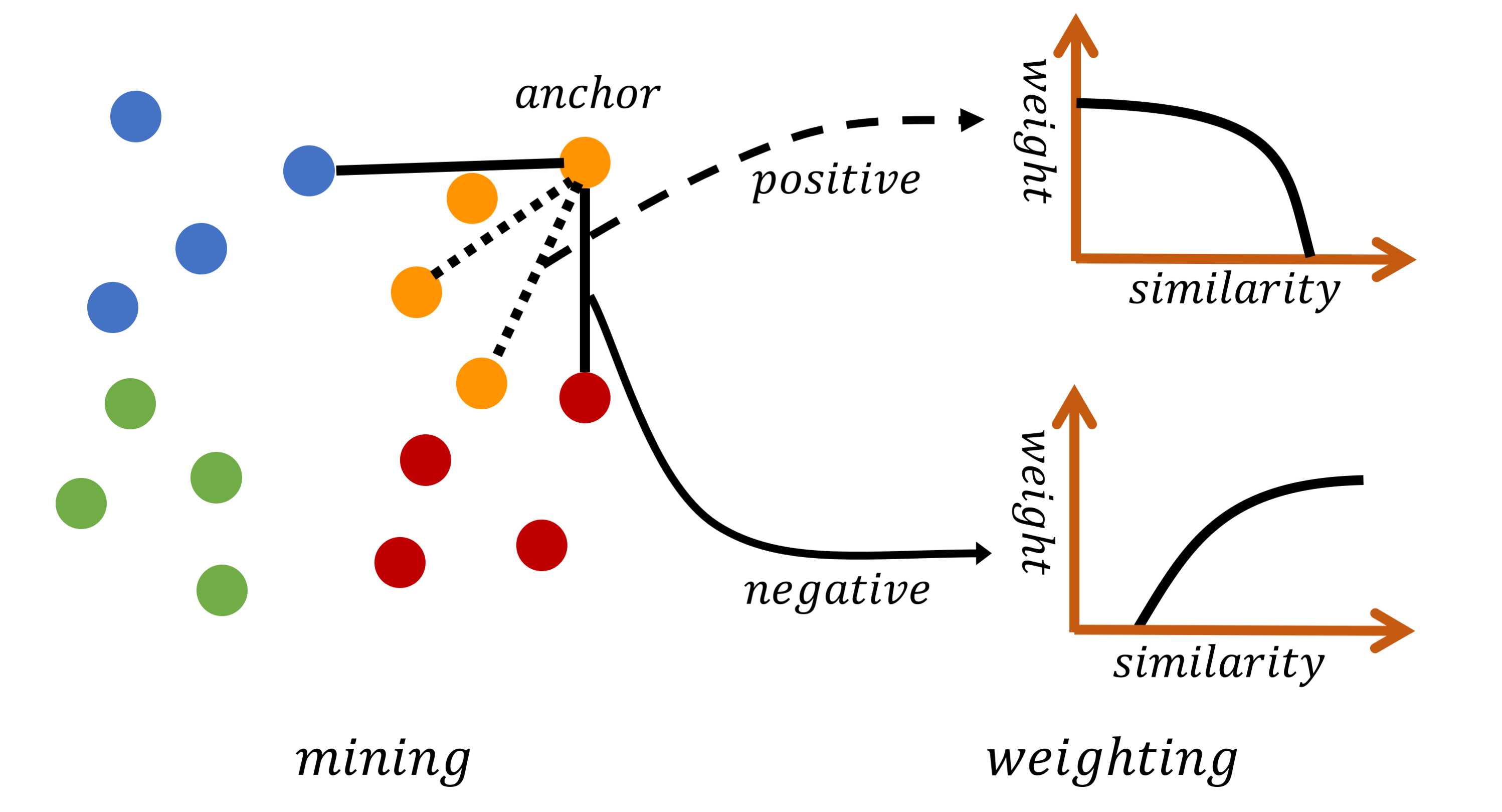
Figure 1: The proposed multi-similarity loss is able to jointly measure the self-similarity and relative similarities of a pair, which allows it collect informative pairs by implementing iterative pair mining and weighting.

Metric learning aims to learn an embedding space, where the embedded vectors of similar samples are encouraged to be closer, while dissimilar ones are pushed apart from each other [22, 23, 39]. With recent great success of deep neural networks in computer vision, deep metric learning has attracted increasing attention, and has been applied to various tasks, including image retrieval [37, 8, 5], face recognition [36], zero-shot learning [42, 1, 15], visual tracking [19, 31] and person re-identification [41, 9].

Many recent deep metric learning approaches are built on pairs of samples. Formally, their loss functions can be expressed in terms of pairwise cosine similarities in the embedding space. We refer to this group of methods as pair-based deep metric learning; and this family includes contrastive loss [6], triplet loss [10], triplet-center loss [8], quadruplet loss [18], lifted structure loss [25], N-pairs loss [29], binomial deviance loss [40], histogram loss [32], angular loss [34], distance weighted margin-based loss [38], hierarchical triplet loss (HTL) [4], etc. For these pair-based methods, training samples are constructed into pairs, triplets or quadruplets, resulting a polynomial growth of training pairs which are highly redundant and less informative. This gives rise to a key issue for pair-based methods, where training with random sampling can be overwhelmed by redundant pairs, leading to slow convergence and model degeneration with inferior performance.

Recent efforts have been devoted to improving sampling schemes for pair-based metric learning techniques. For example, Chopra et al. [3] introduced a contrastive loss which discards negative pairs whose similarities are smaller than a given threshold. In triplet loss [10], a negative pair is sampled by using a margin computed from the similarity of a randomly selected positive pair. Alternatively, lifted structure loss [25] and N-pairs loss [29] introduced new weighting schemes by designing a smooth weighting function to assign a larger weight to a more informative pair. Though driven by different motivations, these methods share a common goal of learning from more informative pairs. Thus, sampling such informative pairs is the key to pair-based deep metric learning, while precisely identifying these pairs is particularly challenging, especially for the negative pairs whose number is quadratic to the size of dataset.

In this work, we cast the sampling problem of deep metric learning into a general pair weighting formulation. We investigated various weighting schemes of recent pair-based loss functions, attempted to understand their insights more deeply, and identify key limitations of these approaches. We observed that a key factor that impacts pair weighting is to compute multiple types of similarities for a pair, which can be defined as self-similarity and relative similarity, where the relative similarity is heavily dependent on the other pairs. Furthermore, we found that most existing methods only explore this factor partially, which limits their capability considerably. For example, contrastive loss [6] and binomial deviance loss [40] only consider the cosine similarity of a pair, while triplet loss [10] and lifted structure loss [25] mainly focus on the relative similarity. We propose a multi-similarity loss which fully considers multiple similarities during sample weighting. The major contributions of this paper are summarized as follows.

• We establish a General Pair Weighting (GPW) framework, which formulates deep metric learning into a unified view of pair weighting. It provides a general formulation for understanding and explaining various pair-based loss functions through gradient analysis.

• We analyze the key factor that impacts pair weighting with GPW, where various pair-based methods can be analyzed comprehensively, with main differences and key limitations clearly identified. This allows us to define three types of similarities for a pair: a self-similarity and two relative similarities. The relative similarities are computed by comparing to other pairs, which are of great importance to existing pair-based methods.

• We propose a new multi-similarity (MS) loss, which is implemented using two iterative steps with sampling and weighting, as shown in Figure 1. MS loss considers both self-similarity and relative similarities which enables the model to collect and weight informative pairs more efficiently and accurately, leading to boosts in performance.

• MS loss is evaluated extensively on a number of benchmarks for image retrieval, where it outperforms current state-of-the-art approaches by a large margin, e.g., improving recent ABE [14] with +5.0% Recall@$1$ on CUB200, and HTL [4] with +7.1% Recall@$1$ on In-Shop Clothes Retrieval dataset.

2 Related Work

Classical pair-based loss functions. Siamese network [6] is a representative pair-based method that learns an embedding via contrastive loss. It encourages samples from a positive pair to be closer, and pushes samples from a negative pair apart from each other, in the embedding space. Triplet loss was introduced in [10] by using triplets as training samples. Each triplet consists of a positive pair and a negative pair by sharing the same anchor point. Triplet loss aims to learn an embedding space where the similarity of a negative pair is lower than that of a positive one, by giving a margin. Extended from triplet loss, quadruplets were also applied in recent work, such as histogram loss [32].

Recently, Song et al. [25] argued that both contrastive loss and triplet loss are difficult to explore full pair-wise relations between samples in a mini-batch. They proposed a lifted structure loss attempted to fully utilize such pairwise relations. However, the lifted structure loss only samples approximately an equal number of negative pairs as the positive ones randomly, and thus discards a large number of informative negative pairs arbitrarily. In [40], Dong et al. proposed a binomial deviance loss by using a binomial deviance to evaluate the cost between labels and similarity, which emphasizes harder pairs. In this work, we propose a multi-similarity loss able to explore more meaningful pair-wise relations by jointly considering both self-similarity and the relative similarities.

Hard sample mining. Pair-based metric learning often generates a large amount of pair-wise samples, which are highly redundant and include many uninformative samples. Training with random sampling can be overwhelmed by these redundant samples, which significantly degrade the model capability and also slows the convergence. Therefore, sampling plays a key role in pair-based metric learning.

The importance of hard negative mining has been discussed extensively [28, 7, 38, 4]. Schroff et al. [28] proposed a semi-hard mining scheme by exploring semi-hard triplets, which are defined to have a negative pair farther than the positive one. However, such semi-hard mining method only generates a small number of valid semi-hard triplets, so that it often requires a large batch-size to generate sufficient semi-hard triplets, e.g., 1800 as suggested in [28]. Harwood et al. [7] provided a framework named smart mining to collect hard samples from the whole dataset, which suffers from off-line computation burden. Recently, Ge et al. [4] proposed a hierarchical triplet loss (HTL) which builds a hierarchical tree of all classes, where hard negative pairs are collected via a dynamic margin. Sampling matters in deep embedding learning was discussed in [38], and a distance weighted sampling was proposed to collect negative samples uniformly with respective to the pair-wise distance. Unlike these methods which mainly focus on sampling or hard sample mining, we provide a more generalized formulation that casts sampling problem into general pair weighting.

Instance weighting. Instance weighting has been widely applied to various tasks. For example, Lin et al. [20] proposed a focal loss that allows the model to focus on hard negative examples during training an object detector. In [2], an active bias learning was developed to emphasize high variance samples in training a neural network for classification. Self-paced learning [17], which pays more attention on samples with a higher confidence, was explored to design noise-robust algorithms [12]. These approaches [20, 13, 2, 17] were developed for weighting individual instances that are only depended on itself (referred as self-similarity), while our method aims to compute both self-similarity and the relative similarities, which is a more complicated problem that requires to measure multiple sample correlations within a local data distribution.

3 General Pair Weighting (GPW)

In this section, we formulate the sampling problem of metric learning into a unified weighting view, and provide a General Pair Weighting (GPW) framework for analyzing various pair-based loss functions.

3.1 GPW Framework

Let ${\bm{x}}_{i}\in\mathbb{R}^{d}$ be a real-value instance vector. Then we have an instance matrix ${\bm{X}}\in\mathbb{R}^{m\times d}$, and a label vector ${\bm{y}}\in\{1,2,\dots,C\}^{m}$ for the $m$ training samples respectively. Then an instance ${\bm{x}}_{i}$ is projected onto a unit sphere in a $l$-dimension space by $f(\cdot;{\bm{\theta}}):\mathbb{R}^{d}\rightarrow S^{l}$, where $f$ is a neural network parameterized by ${\bm{\theta}}$. Formally, we define the similarity of two samples as $S_{ij}\mathrel{\vbox{\hbox{\scriptsize.}\hbox{\scriptsize.}}}=<f({\bm{x}}_{i};{\bm{\theta}}),f({\bm{x}}_{j};{\bm{\theta}})>$, where $<\cdot,\cdot>$ denotes dot product, resulting in an $m\times m$ similarity matrix ${\bm{S}}$ whose element at $(i,j)$ is $S_{ij}$.

Given a pair-based loss $\mathcal{L}$, it can be formulated as a function in terms of ${\bm{S}}$ and ${\bm{y}}$: $\mathcal{L}({\bm{S}},{\bm{y}})$. The derivative with respect to model parameters ${\bm{\theta}}$ at the $t$-th iteration can be calculated as:

$$\begin{split}\frac{\partial\mathcal{L}({\bm{S}},{\bm{y}})}{\partial{\bm{\theta}}}\bigg{|}_{t}&{}=\frac{\partial\mathcal{L}({{\bm{S}},{\bm{y}}})}{\partial{\bm{S}}}\bigg{|}_{t}\quad\frac{\partial{{\bm{S}}}}{\partial{\bm{\theta}}}\bigg{|}_{t}\\ &{}=\sum_{i=1}^{m}\sum_{j=1}^{m}\frac{\partial\mathcal{L}({\bm{S}},{\bm{y}})}{\partial S_{ij}}\bigg{|}_{t}\quad\frac{\partial{S_{ij}}}{\partial{\bm{\theta}}}\bigg{|}_{t}.\end{split}$$ (1)

Eqn 1 is computed for optimizing model parameters ${\bm{\theta}}$ in deep metric learning. In fact, Eqn 1 can be reformulated into a new form for pair weighting through a new function $\mathcal{F}$, whose gradient w.r.t. ${\bm{\theta}}$ at the $t$-th iteration is computed exactly the same as Eq. 1. $\mathcal{F}$ is formulated as below:

$$\mathcal{F}({\bm{S}},{\bm{y}})=\sum_{i=1}^{m}\sum_{j=1}^{m}\frac{\partial\mathcal{L}({\bm{S}},{\bm{y}})}{\partial S_{ij}}\bigg{|}_{t}S_{ij}.$$ (2)

Note that $\frac{\partial\mathcal{L}({\bm{S}},{\bm{y}})}{\partial S_{ij}}\big{|}_{t}$ is regarded as a constant scalar that not involved in the gradient of $\mathcal{F}$ w.r.t. ${\bm{\theta}}$.

Since the central idea of deep metric learning is to encourage positive pairs to be closer, and push negatives apart from each other. For a pair-based loss $\mathcal{L}$, we can assume $\frac{\partial\mathcal{L}({\bm{S}},{\bm{y}})}{\partial S_{ij}}\big{|}_{t}\geqslant 0$ for a negative pair, and $\frac{\partial\mathcal{L}({\bm{S}},{\bm{y}})}{\partial S_{ij}}\big{|}_{t}\leqslant 0$ for a positive pair. Thus, $\mathcal{F}$ in Eqn 2 can be transformed into the form of pair weighting as follows:

$$\begin{split}\mathcal{F}&{}=\sum_{i=1}^{m}\left(\sum_{{\bm{y}}_{j}\neq{\bm{y}}_{i}}^{m}\frac{\partial\mathcal{L}({\bm{S}},{\bm{y}})}{\partial S_{ij}}\bigg{|}_{t}S_{ij}+\sum_{{\bm{y}}_{j}={\bm{y}}_{i}}^{m}\frac{\partial\mathcal{L}({\bm{S}},{\bm{y}})}{\partial S_{ij}}\bigg{|}_{t}S_{ij}\right)\\ &{}=\sum_{i=1}^{m}\left(\sum_{{\bm{y}}_{j}\neq{\bm{y}}_{i}}^{m}w_{ij}S_{ij}-\sum_{{\bm{y}}_{j}={\bm{y}}_{i}}^{m}w_{ij}S_{ij}\right),\end{split}$$ (3)

where $w_{ij}=\bigg{|}\frac{\partial\mathcal{L}({\bm{S}},{\bm{y}})}{\partial S_{ij}}\big{|}_{t}\bigg{|}$.

As indicted in Eqn 3, a pair-based method can be formulated as weighting of pair-wise similarities, where the weight for pair $\{{\bm{x}}_{i},{\bm{x}}_{j}\}$ is $w_{ij}$. Learning with a pair-based loss function $\mathcal{L}$ is now transformed from Eq. 1 into designing weights for pairs. It is a general pair weighting (GPW) formulation, and sampling is only a special cases.

3.2 Revisit Pair-based Loss Functions

To demonstrate the generalization ability of GPW framework, we revisit four typical pair-based loss functions for deep metric learning: contrastive loss [6],， triplet loss [10], binomial deviance loss [40] and lifted structure loss [25].

Contrastive loss. Hadsell et al. [6] proposed a Siamese network, where a contrastive loss was designed to encourage positive pairs to be as close as possible, and negative pairs to be apart from each other over a given threshold, $\lambda$:

$$\mathcal{L}_{contrast}\mathrel{\vbox{\hbox{\scriptsize.}\hbox{\scriptsize.}}}=(1-\mathcal{I}_{ij})[S_{ij}-\lambda]_{+}-\mathcal{I}_{ij}S_{ij},$$ (4)

where $\mathcal{I}_{ij}=1$ indicates a positive pair, and $0$ for a negative one. By computing partial derivative with respect to $S_{ij}$ in Eqn 4, we can find that all positive pairs and hard negative pairs with $S_{ij}>\lambda$ are assigned with an equal weight. This is a simple and special case of our pair weighting scheme, without considering any difference between the selected pairs.

Triplet loss. In [10], a triplet loss was proposed to learn a deep embedding, which enforces the similarity of a negative pair to be smaller than that of a randomly selected positive one over a given margin $\lambda$:

$$\mathcal{L}_{triplet}\coloneqq[S_{an}-S_{ap}+\lambda]_{+},$$ (5)

where $S_{an}$ and $S_{ap}$ denote the similarity of a negative pair $\{{\bm{x}}_{a},{\bm{x}}_{n}\}$, and a positive pair $\{{\bm{x}}_{a},{\bm{x}}_{p}\}$, with an anchor sam, e$pl{\bm{x}}_{a}$. According to the gradient computed for Eqn 5, a triplet loss weights all pairs equally on the valid triplets which are selected by $S_{an}+\lambda>S_{ap}$, while the triplets with $S_{an}+\lambda\leqslant S_{ap}$ are considered as less informative, and are discarded. Triplet loss is different from contrastive loss on pair selection scheme, but both methods consider all the selected pairs equally, which limits their ability to identify more informative pairs among the selected ones.

Lifted Structure Loss. Song et al. [25] designed a lifted structure loss, which was further improved to a more generalized version in [9]. It utilizes all the positive and negative pairs among the mini-batch as follows:

$$\mathcal{L}_{lifted}\mathrel{\vbox{\hbox{\scriptsize.}\hbox{\scriptsize.}}}=\sum_{i=1}^{m}\bigg{[}{\log\sum_{{\bm{y}}_{k}={\bm{y}}_{i}}e^{\lambda-S_{ik}}}+\log\sum_{{\bm{y}}_{k}\neq{\bm{y}}_{i}}e^{S_{ik}}\bigg{]}_{+},$$ (6)

where $\lambda$ is a fixed margin.

In Eqn 6, when the hinge function of an anchor ${\bm{x}}_{i}$ returns a non-zero value, we can have a weight value, $w_{ij}$, for the pair $\{{\bm{x}}_{i},{\bm{x}}_{j}\}$, by differentiating $\mathcal{L}_{lifted}$ on $S_{ij}$, according to Eqn 3. Then the weight for a positive pair is computed as:

$$w^{+}_{ij}=\frac{e^{\lambda-S_{ij}}}{\sum_{{\bm{y}}_{k}={\bm{y}}_{i}}e^{\lambda-S_{ik}}}=\frac{1}{\sum_{{\bm{y}}_{k}={\bm{y}}_{i}}e^{S_{ij}-S_{ik}}},$$ (7)

and the weight for a negative pair is:

$$w^{-}_{ij}=\frac{e^{S_{ij}}}{\sum_{{\bm{y}}_{k}\neq{\bm{y}}_{i}}e^{S_{ik}}}=\frac{1}{\sum_{{\bm{y}}_{k}\neq{\bm{y}}_{i}}e^{S_{ik}-S_{ij}}}.$$ (8)

Eqn 7 shows that the weight for a positive pair is determined by its relative similarity, measured by comparing it to the remained positive pairs with the same anchor. The weight for a negative pair is computed similarly based on Eqn 8.

Binomial Deviance Loss. Dong et al. introduced binomial deviance loss in [40], which utilizes softplus function instead of hinge function in contrastive loss:

$$\begin{split}\mathcal{L}_{binomial}=\sum_{i=1}^{m}\bigg{\{}&{}\frac{1}{{P_{i}}}{\sum_{{\bm{y}}_{j}={\bm{y}}_{i}}\log\left[1+e^{\alpha(\lambda-S_{ij})}\right]}+\\ &{}\frac{1}{N_{i}}\sum_{{\bm{y}}_{j}\neq{\bm{y}}_{i}}\log\left[1+e^{\beta(S_{ij}-\lambda)}\right]\bigg{\}},\end{split}$$ (9)

where ${P_{i}}$ and ${N_{i}}$ denote the numbers of positive pairs and negative pairs with anchor ${\bm{x}}_{i}$, respectively. $\lambda$, $\alpha$, $\beta$ are fixed hyper-parameters.

The weight for pair $\{{\bm{x}}_{i},{\bm{x}}_{j}\}$ is $w_{ij}$ in Eqn 1, which can be derived from differentiating $\mathcal{L}_{binomial}$ on $S_{ij}$ as:

$$\begin{split}w^{+}_{ij}&{}=\frac{1}{P_{i}}\frac{\alpha e^{\alpha\left(\lambda-S_{ij}\right)}}{1+e^{\alpha\left(\lambda-S_{ij}\right)}},\quad\quad{\bm{y}}_{j}={\bm{y}}_{i}\\ w^{-}_{ij}&{}=\frac{1}{N_{i}}\frac{\beta e^{\beta\left(S_{ij}-\lambda\right)}}{1+e^{\beta\left(S_{ij}-\lambda\right)}},\quad\quad{\bm{y}}_{j}\neq{\bm{y}}_{i}\end{split}$$ (10)

As can be found, binomial deviance loss is a soft version of contrastive loss. In Eqn 3, a negative pair with a higher similarity is assigned with a larger weight, which means that it is more informative, by distinguishing two similar samples from different classes (which form a negative pair).

4 Multi-Similarity Loss

In this section, we first illustrate three types of similarities that carries the information of pairs, and then design a multi-similarity loss that weighting pairs based on full information.

4.1 Multiple Similarities

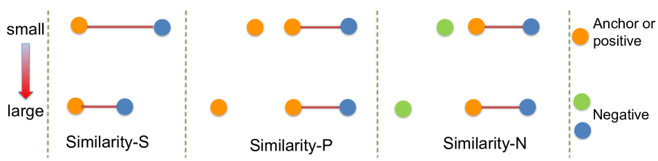
Figure 2: Three types of similarities of a negative pair. From left to right, S: its cosine similarity to the anchor; P: its relative similarity compared with the positive pair; N: its relative similarity compared with other negative pairs. From top to bottom, the similarities becomes higher. Their weights should be larger since they contains more information to improve the current model.

	Contrastive	Binomial	Triplet	Histogram	N-pairs	Lifted Structure	BinLifted	NCA	MS
Similarity-S	✓	✓	✗	✗	✗	✗	✓	✗	✓
Similarity-P	✗	✗	✓	✓	✗	✗	✗	✓	✓
Similarity-N	✗	✗	✗	✗	✓	✓	✓	✓	✓

Table 1: The types of similarities considered by the pair-based methods on weighting negative pairs. In the table, we can find that most existing pair-based methods only consider the three types of similarities partly, while our MS loss weights the negative pairs by considering all the three perspectives comprehensively.

Based on GPW, we can find that most pair-based approaches weight the pairs based on either self cosine similarities or relative similarities compared with other pairs. Specifically, we take one negative pair for example and summarize three types of similarities as below. (The analysis of one positive pair is in a similar way.)

Similarity-S: Self-similarity defined as the cosine similarity between the negative sample and the anchor is of the most importance. A negative pair with a larger self similarity means that it is harder to distinguish two paired samples from different classes. Such pairs are referred as hard negative pairs, which are more informative and meaningful to learn discriminative features. Contrastive loss and binomial deviance loss are based on this criterion. In the left of Figure 2, the weight of the negative pair in Eq n 10 increases, since the pair’s self similarity grows larger as the pair becomes closer.

In fact, self-similarity is not able to fully evaluate the value of a negative pair solely, and correlations of other pairs also make significant impact to weight assignment. Thus, We further introduce two types of relative similarities by considering all other pairs to exploit the potentiality of each pair.

Similarity-P: Positive relative similarity is computed by considering the relationship with positive pairs. Specifically, we define it as the differences of its own cosine similarity and that of other positive pairs. In the middle of Figure 2, the Similarity-P stays the same, while Similarity-P increases as the positive pair becomes faraway. Obviously, such case brings more challenge of retrieve the right sample for the anchor, as the negative pair is more closer than the positive. Thus, the negative pair should assigned more weight to learn an embedding. Triplet loss and histogram loss are based on Similarity-P.

Similarity-N: Negative relative similarity is the differences between its cosine similarity and those of other negative pairs. In the right of Figure 2, the Similarity-N of the negative pair becomes larger, while its self-similarity is fixed. Indeed, when the Similarity-N become larger, the pair carries more valuable information compared with other negatives. Thus, to learn a good embedding, we should focus weights on such pairs. Lifted structure, N-pairs and NCA methods assign weights for each negative pair according to Similarity-N.

With the GPW, we analyze the weighting schemes of most existing pair-based approaches, and summarize the similarities they depends on in weighting (in Table 1). We observe that these commonly used pair-based methods only rely on partial similarities, which cannot cover the information contained in current pair. For example, lifted structure method only considers N-similarity, compares current pair with other negative pairs for weighting. The weight of current pair will be unchanged when the S-similarity becomes larger (in the left of Fig. 2) or when negative samples depart from the anchor (in the right of Fig. 2). This conclusion can also be verified directly from Eqn 8, which only depends on the term: $\sum_{{\bm{y}}_{k}={\bm{y}}_{i}}e^{S_{ij}-S_{ik}}$. Thus, to properly weighting one pair, not only the S-similarity should be taken into account, but also the P-similarity and N-similarity.

While a weighting or sampling method based on each individual similarity has been explored previously, to the best of our knowledge, none of existing pair-based methods assign weights on pairs considering all the three similarities. In the following, we propose our MS loss, whose weighting strategy is designed by taking a general consideration of all the three types of similarities.

4.2 Multi-Similarity Loss

Unlike sampling or weighting schemes developed for classification and detection tasks ([2, 20]), where the weight of an instance is computed individually based on itself, it is difficult to precisely measure the informativeness of a pair based on itself individually in deep metric learning. Relationships with relevant samples or pairs should also be considered to make the measurement more accurate.

However, to the best our knowledge, none of the existing pair-based methods can consider all of the three similarities simultaneously (in table 1). To this end, we propose a Multi-Similarity (MS) loss, which consider all three perspectives by implementing a new pair weighting scheme using two steps: mining and weighting. (i) informative pairs are first sampled by measuring Similarity-P; and then (ii) the selected pairs are further weighted using Similarity-S and Similarity-N jointly. Details of the two steps are described as follows.

Pair mining. We first select informative pairs by computing Similarity-P, which measures the relative similarity between negative$\leftrightarrow$positive pairs having a same anchor. Specifically, a negative pair is compared to the hardest positive pair (with the lowest similarity), while a positive pair is sampled by comparing to a negative one having the largest similarity. Formally, assume ${\bm{x}}_{i}$ is an anchor, a negative pair $\{{\bm{x}}_{i},{\bm{x}}_{j}\}$ is selected if $S_{ij}$ satisfies the condition:

$$S^{-}_{ij}>\min_{{\bm{y}}_{k}={\bm{y}}_{i}}S_{ik}-\epsilon,$$ (11)

where $\epsilon$ is a given margin.

If $\{{\bm{x}}_{i},{\bm{x}}_{j}\}$ is a positive pair, the condition is:

$$S^{+}_{ij}<\max_{{\bm{y}}_{k}\neq{\bm{y}}_{i}}S_{ik}+\epsilon.$$ (12)

For an anchor ${\bm{x}}_{i}$, we denote the index set of its selected positive and negative pairs as $\mathcal{P}_{i}$ and $\mathcal{N}_{i}$ respectively. Our hard mining strategy is inspired by large margin nearest neighbor (LMNN) [35], a traditional distance learning approach which targets to seek an embedding space where neighboring positive points are encouraged to have the same class label with the anchor. The negative samples that satisfy Eqn 11 are approximately identical to impostors defined in LMNN [35].

Pair weighting. Pair mining with Similarity-P can roughly select informative pairs, and discard the less informative ones. We develop a soft weighting scheme that further weights the selected pairs more accurately, by considering both Similarity-S and Similarity-N. Our weighting mechanism is inspired by binomial deviance loss (considering similarity-S) and lifted structure loss (using Similarity-N). Specifically, given a selected negative pair $\{{\bm{x}}_{i},{\bm{x}}_{j}\}\in\mathcal{N}_{i}$, its weight $w_{ij}^{-}$ can be computed as:

$$\begin{split}w^{-}_{ij}&{}=\frac{1}{e^{\beta\left(\lambda-S_{ij}\right)}+\sum\limits_{k\in\mathcal{N}_{i}}e^{\beta\left(S_{ik}-S_{ij}\right)}}\\ &{}=\frac{e^{\beta\left(S_{ij}-\lambda\right)}}{1+\sum\limits_{k\in\mathcal{N}_{i}}e^{\beta\left(S_{ik}-\lambda\right)}}.\end{split}$$ (13)

and the weight $w_{ij}^{+}$ of a positive pair $\{{\bm{x}}_{i},{\bm{x}}_{j}\}\in\mathcal{P}_{i}$ is:

$$\begin{split}w^{+}_{ij}&{}=\frac{1}{e^{-\alpha\left(\lambda-S_{ij}\right)}+\sum\limits_{k\in\mathcal{P}_{i}}e^{-\alpha\left(S_{ik}-S_{ij}\right)}},\end{split}$$ (14)

where $\alpha,\beta,\lambda$ are hyper-parameters as in Binomial deviance loss (Eqn 9).

In Eqn 13, the weight of a negative pair is computed jointly from its self-similarity by $e^{\beta\left(\lambda-S_{ij}\right)}$ - Similarity-S, and its relative similarity - Similarity-N, by comparing to its negative pairs. Similar rules are applied for computing the weight for a positive pair, as in Eqn 14. With these two considerations, our weighting scheme updates the weights of pairs dramatically to the violation of its self-similarity and relative similarities.

The weight computed by Eqn 13 and Eqn 14 can be considered as a combination of the weight formulations of binomial deviance loss and lifted structure loss. However, it is non-trivial to combine both functions in an elegant and suitable manner. We will compare our MS weighting with an average weighting scheme of binomial deviance (Eqn 10) and lifted structure (Eqn 8), denoted as BinLifted. We demonstrate by experiments that direct combination of them can not lead to performance improvement (as shown in ablation study).

Finally, we integrate pair mining and weighting scheme into a single framework, and provide a new pair-based loss function - multi-similarity (MS) loss, whose partial derivative with respect to $S_{ij}$ is the weight defined in Eqn 13 and Eqn 14. Our MS loss is formulated as,

$$\begin{split}\mathcal{L}_{MS}=\frac{1}{m}\sum_{i=1}^{m}\bigg{\{}\frac{1}{\alpha}{\log\big{[}1+\sum_{k\in\mathcal{P}_{i}}e^{-\alpha(S_{ik}-\lambda)}}\big{]}\\ +\frac{1}{\beta}{\log\big{[}1+\sum_{k\in\mathcal{N}_{i}}e^{\beta(S_{ik}-\lambda)}\big{]}}\bigg{\}}.\end{split}$$ (15)

where $\mathcal{L}_{MS}$ can be minimized with gradient descent optimization, by simply implementing the proposed iterative pair mining and weighting.

5 Experiments

Our MS method is implemented by PyTorch. For network architecture, we use the Inception network with batch normalization [11] pre-trained on ILSVRC 2012-CLS [27], and fine-tuned it for our task. We add a FC layer on the top of the network following the global pooling layer. All the input images are cropped to $224\times 224$. Random crop with random horizontal flip is used for training, and single center crop for testing. Adam optimizer was used for all experiments.

We conduct experiments on four standard datasets: CUB200 [33], Cars-196 [16], Stanford Online Products (SOP) [25] and In-Shop Clothes Retrieval (In-Shop) [21]. We follow the data split protocol applied in [25]. For the CUB200 dataset, we use the first 100 classes with 5,864 images for training, and the remaining 100 classes with 5,924 images for testing. The Cars-196 dataset is composed of 16,185 images of cars from 196 model categories. The first 98 model categories are used for training, with the rest for testing. For the SOP dataset, we use 11,318 classes for training, and 11,316 classes for testing. For the In-Shop dataset, 3,997 classes with 25,882 images are used for training. The test set is partitioned to a query set with 14,218 images of 3,985 classes, and a gallery set having 3,985 classes with 12,612 images.

For every mini-batch, we randomly choose a certain number of classes, and then randomly sample $M$ instances from each class with $M=5$ for all datasets in all experiments. $\epsilon$ in Eqn 11 and Eqn 12 is set to $0.1$ and the hyper-parameters in Eqn 15 are: $\alpha=2,\lambda=1,\beta=50$, by following [32]. Our method is evaluated on image retrieval task by using the standard performance metric: Recall$@K$.

Recall$@K$ (%)		1	2	4	8
Binomial	S	71.9	80.0	86.4	91.0
LiftedStruct∗	N	69.7	79.3	86.2	91.0
MS mining	P	67.0	77.4	84.7	90.0
BinLifted	SN	70.4	79.5	86.2	91.1
MS weighting	SN	73.2	81.5	87.6	92.6
Binomialm	SP	74.6	83.8	89.7	94.1
LiftedStruct${}_{m}^{*}$	NP	72.2	81.7	88.0	92.4
MS	SNP	77.3	85.3	90.5	94.2

Table 2: Results on Cars-196 using different pair-based methods. The first column lists the methods and the types of similarities considered in their weighting. Embedding size is set to 64. Subscript ${m}$ denotes applying our MS mining step before weighting.

5.1 Ablation Study

To demonstrate the importance of weighting the pairs from multi-similarities, we conduct an ablation study on Cars-196 and results are shown in Table 2. We describe LiftedStruct^∗, MS mining and MS weighting here, other methods have already been mentioned in section 3.

LiftedStruct^∗. Lifted structure loss is easy to get stuck in a local optima, resulting in poor performance. To evaluate the efficiency of three similarities more clearly and fairly, we make a minor modification to the lifted structure loss, allowing it to employ Similarity-N more effectively:

$$\small\mathcal{L}_{lift*}=\frac{1}{m}\sum_{i=1}^{m}\bigg{\{}\frac{1}{\alpha}{\log\sum_{{\bm{y}}_{k}={\bm{y}}_{i}}e^{-\alpha S_{ik}}}+\frac{1}{\beta}{\log\sum_{{\bm{y}}_{k}\neq{\bm{y}}_{i}}e^{\beta S_{ik}}}\bigg{\}},$$ (16)

where $\alpha=2$, $\beta=50$. This modification is motivated to make lift structure loss more focus on informative pairs, especially the hard negative pairs, and allows it to get rid of the side effect of enormous easy negative pairs. We found that this modification can boost the performance of lifted-structure loss empirically, e.g., with an over 20% improvement of Recall@1 on the CUB200 .

MS mining. To investigate the impact of each component of MS Loss, we evaluate the performance of MS mining individually, where the pairs selected into $\mathcal{N}_{i}$ and $\mathcal{P}_{i}$ are assigned with an equal weight.

MS weighting. Similarly, MS weighting scheme is also evaluated individually without the mining step in the ablation study, allowing us to analyze the effect of each similarity more perspicaciously. In MS weighting, each pair in a mini-batch is assigned with a non-zero weight, according to the weighting strategy described in Eqn 13 and Eqn 14.

With the performance reported in Table 2, we analyze the effect of each similarity as below:

Similarity-S: A cosine self-similarity is of the most importance. Binomial deviance loss, based on the Similarity-S, achieves the best performance by using a single similarity. Moreover, our MS weighting outperforms LiftedStruct${}_{m}^{*}$ by $69.7\%\rightarrow 73.2\%$ at recall@1, and Binomial_m also improves the recall@1 with $67.0\%\rightarrow 74.6\%$ over the MS mining, by adding the Similarity-S into their weighting schemes.

Similarity-N: Relative similarities are also helpful to measuring the importance of a pair more precisely. With Similarity-N, our MS weighting increases the Recall@1 by 1.3% over Binomial ($71.9\%\rightarrow 73.2\%$). Moreover, with Similarity-N, LiftedStruct${}_{m}^{*}$ obtains a significant performance improvement over MS sampling ($67\%\rightarrow 72.2\%$), by considering both Similarity-P and Similarity-N.

Similarity-P: As shown in Table 2, by adding a mining step based on Similarity-P, the performances of LiftedStruct^∗, Binomial and MS weighting are consistently improved by a large margin. For instance, Recall@1 of Binomial is increased by nearly 3%: $71.9\%\rightarrow 74.6\%$.

Finally, the proposed MS loss achieves the best performance among these methods, by exploring multi-similarities for pair mining and weighting. However, it is critical to integrate the three similarities effectively into a single framework where the three similarities can be fully explored and optimized jointly by using a single loss function. For example, BinLifted, which uses a weighting scheme considering both similarities-S and similarities-N, has lower performance than that of single Binomial, since it implements a simple and straightforward combination of Binomial and LiftedStruct${}_{m}^{*}$. More discussions on the difference between our MS weighting and the direct combination are presented in Supplementary Material.

	CUB-200-2011						Cars-196
Recall$@K$ (%)	1	2	4	8	16	32	1	2	4	8	16	32
Clustering 64[30]	48.2	61.4	71.8	81.9	-	-	58.1	70.6	80.3	87.8	-	-
ProxyNCA64 [24]	49.2	61.9	67.9	72.4	-	-	73.2	82.4	86.4	87.8	-	-
Smart Mining64 [7]	49.8	62.3	74.1	83.3	-	-	64.7	76.2	84.2	90.2	-	-
Margin128 [38]	63.6	74.4	83.1	90.0	94.2	-	79.6	86.5	91.9	95.1	97.3	-
HDC384 [30]	53.6	65.7	77.0	85.6	91.5	95.5	73.7	83.2	89.5	93.8	96.7	98.4
HTL512 [4]	57.1	68.8	78.7	86.5	92.5	95.5	81.4	88.0	92.7	95.7	97.4	99.0
ABIER512 [26]	57.5	68.7	78.3	86.2	91.9	95.5	82.0	89.0	93.2	96.1	97.8	98.7
ABE512 [14]	60.6	71.5	79.8	87.4	-	-	85.2	90.5	94.0	96.1	-	-
MS64	57.4	69.8	80.0	87.8	93.2	96.4	77.3	85.3	90.5	94.2	96.9	98.2
MS512	65.7	77.0	86.3	91.2	95.0	97.3	84.1	90.4	94.0	96.5	98.0	98.9

Table 3: Recall@$K(\%)$ performance on CUB200 and Cars-196. Superscript denotes embedding size. ABIER [26] and ABE [14] are ensemble methods.

5.2 On Embedding Size

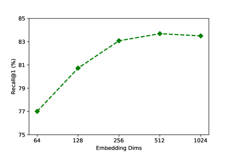
Figure 3: Results on the Cars-196 dataset using different embedding sizes of our MS loss. Larger embedding size can considerably improve recall@1, while embedding sizes larger than 512 are not necessary.

By following [28], we study the performance of MS loss with varying embedding sizes $\{64,128,256,512,1024\}$. As shown in Figure 3, the performance is increased consistently with the embedding dimension except at 1024. This is different from lifted structure loss, which achieves its best performance at 64 on the Cars-196 dataset [25].

Recall$@K$ (%)	1	10	20	30	40	50
FashionNet4096 [21]	53.0	73.0	76.0	77.0	79.0	80.0
HDC384 [30]	62.1	84.9	89.0	91.2	92.3	93.1
HTL128 [4]	80.9	94.3	95.8	97.2	97.4	97.8
ABIER512 [26]	83.1	95.1	96.9	97.5	97.8	98.0
ABE512 [14]	87.3	96.7	97.9	98.2	98.5	98.7
MS128	88.0	97.2	98.1	98.5	98.7	98.8
MS512	89.7	97.9	98.5	98.8	99.1	99.2

Table 4: Recall@$K(\%)$ performance on In-Shop.

5.3 Comparison with State-of-the-Art

Recall$@K$ (%)	1	10	100	1000
Clustering 64[30]	67.0	83.7	93.2	-
ProxyNCA64 [24]	73.7	-	-	-
Margin128 [38]	72.7	86.2	93.8	98.0
HDC384 [30]	69.5	84.4	92.8	97.7
HTL 512 [4]	74.8	88.3	94.8	98.4
ABIER512 [26]	74.2	86.9	94.0	97.8
ABE512 [14]	76.3	88.4	94.8	98.2
MS64	74.1	87.8	94.7	98.2
MS128	76.6	89.2	95.2	98.4
MS512	78.2	90.5	96.0	98.7

Table 5: Recall@$K(\%)$ performance on SOP.

We further compare the performance of our method with the state-of-the-art techniques on image retrieval task. As shown in Table 3, our MS loss improves Recall@1 by 7% on the CUB200, and 4% on the Cars-196 over Proxy-NCA at dimension 64. Compared with ABE employing an embedding size of 512 and attention modules, our MS loss achieves a higher Recall@1 by +5% improvement at the same dimension on the CUB200. On the Cars-196, our MS loss obtains the second best performance in terms of Recall@1, while the best results are achieved by ABE, which applies an ensemble method with a much heavier model. Moreover, on the remaining three datasets, our MS loss is of much stronger performance than ABE.

In Table 4 and 5, our MS loss outperforms Proxy-NCA by 0.4% and Clustering by 7% at the same embedding size of 64. Furthermore, when compared with ABE, MS loss increases Recall@1 by 1.9% and 2.7% on the SOP and In-Shop respectively. Moreover, even with much compact embedding features of 128 dimension, our MS loss has already surpassed all existing methods, which utilize much higher dimensions of 384, 512 and 4096.

To summarize, on both fine-grained datasets like Cars-196 and CUB200, and large-scale datasets with enormous categories like SOP and In-Shop, our method achieves new state-of-the-art or comparable performance, even taking those methods with ensemble techniques like ABE and BIER into consideration.

6 Conclusion

We have established a General Pair Weighting (GPW) framework and presented a new multi-similarity loss to fully exploit the information of each pair. Our GPW, for the first time, unifies existing pair-based metric learning approaches into general pair weighting through gradient analysis. It provides a powerful tool for understanding and explaining various pair-based loss functions, which allows us to clearly identify the main differences and key limitations of existing methods. Furthermore, we proposed a multi-similarity loss which considers all three similarities simultaneously, and developed an iterative pair mining and weighting scheme for optimizing the multi-similarity loss efficiently. Our method obtains new state-of-the-art performance on a number of image retrieval benchmarks.

See pages 1 of 2333-supp.pdf See pages 2 of 2333-supp.pdf See pages 3 of 2333-supp.pdf

References

- [1] M. Bucher, S. Herbin, and F. Jurie. Improving semantic embedding consistency by metric learning for zero-shot classiffication. In ECCV, 2016.
- [2] H.-S. Chang, E. Learned-Miller, and A. McCallum. Active bias: Training more accurate neural networks by emphasizing high variance samples. In NIPS, 2017.
- [3] S. Chopra, R. Hadsell, and Y. LeCun. Learning a similarity metric discriminatively, with application to face verification. In CVPR, 2005.
- [4] W. Ge, W. Huang, D. Dong, and M. R. Scott. Deep metric learning with hierarchical triplet loss. In ECCV, 2018.
- [5] A. Grabner, P. M. Roth, and V. Lepetit. 3d pose estimation and 3d model retrieval for objects in the wild. In CVPR, 2018.
- [6] R. Hadsell, S. Chopra, and Y. LeCun. Dimensionality reduction by learning an invariant mapping. In CVPR, 2006.
- [7] B. Harwood, V. K. B G, G. Carneiro, I. Reid, and T. Drummond. Smart mining for deep metric learning. In ICCV, 2017.
- [8] X. He, Y. Zhou, Z. Zhou, S. Bai, and X. Bai. Triplet-center loss for multi-view 3d object retrieval. In CVPR, 2018.
- [9] A. Hermans*, L. Beyer*, and B. Leibe. In defense of the triplet loss for person re-identification. arXiv:1703.07737v4, 2017.
- [10] E. Hoffer and N. Ailon. Deep metric learning using triplet network. In SIMBAD, 2015.
- [11] S. Ioffe and C. Szegedy. Batch normalization: Accelerating deep network training by reducing internal covariate shift. In ICML, 2015.
- [12] L. Jiang, D. Meng, S.-I. Yu, Z. Lan, S. Shan, and A. Hauptmann. Self-paced learning with diversity. In NIPS. 2014.
- [13] L. Jiang, Z. Zhou, T. Leung, L.-J. Li, and L. Fei-Fei. Mentornet: Learning data-driven curriculum for very deep neural networks on corrupted labels. In ICML, 2018.
- [14] W. Kim, B. Goyal, K. Chawla, J. Lee, and K. Kwon. Attention-based ensemble for deep metric learning. In ECCV, 2018.
- [15] S. Kiran Yelamarthi, S. Krishna Reddy, A. Mishra, and A. Mittal. A zero-shot framework for sketch based image retrieval. In ECCV, 2018.
- [16] J. Krause, M. Stark, J. Deng, and L. Fei-Fei. 3d object representations for fine-grained categorization. In ICCV Workshops, 2013.
- [17] M. P. Kumar, B. Packer, and D. Koller. Self-paced learning for latent variable models. In NIPS, 2010.
- [18] M. T. Law, N. Thome, and M. Cord. Quadruplet-wise image similarity learning. In ICCV, 2013.
- [19] L. Leal-Taixé, C. Canton-Ferrer, and K. Schindler. Learning by tracking: Siamese cnn for robust target association. In CVPR Workshops, 2016.
- [20] T.-Y. Lin, P. Goyal, R. Girshick, K. He, and P. Dollar. Focal loss for dense object detection. In ICCV, 2017.
- [21] Z. Liu, P. Luo, S. Qiu, X. Wang, and X. Tang. Deepfashion: Powering robust clothes recognition and retrieval with rich annotations. In CVPR, 2016.
- [22] D. G. Lowe. Similarity metric learning for a variable-kernel classifier. Neural computation, 1995.
- [23] S. Mika, G. Ratsch, J. Weston, B. Scholkopf, and K.-R. Mullers. Fisher discriminant analysis with kernels. In Neural networks for signal processing, 1999.
- [24] Y. Movshovitz-Attias, A. Toshev, T. K. Leung, S. Ioffe, and S. Singh. No fuss distance metric learning using proxies. In ICCV, 2017.
- [25] H. Oh Song, Y. Xiang, S. Jegelka, and S. Savarese. Deep metric learning via lifted structured feature embedding. In CVPR, 2016.
- [26] M. Opitz, G. Waltner, H. Possegger, and H. Bischof. Deep Metric Learning with BIER: Boosting Independent Embeddings Robustly. PAMI, 2018.
- [27] O. Russakovsky, J. Deng, H. Su, J. Krause, S. Satheesh, S. Ma, Z. Huang, A. Karpathy, A. Khosla, M. Bernstein, A. C. Berg, and L. Fei-Fei. ImageNet Large Scale Visual Recognition Challenge. IJCV, 2015.
- [28] F. Schroff, D. Kalenichenko, and J. Philbin. Facenet: A unified embedding for face recognition and clustering. In CVPR, 2015.
- [29] K. Sohn. Improved deep metric learning with multi-class n-pair loss objective. In NIPS. 2016.
- [30] H. O. Song, S. Jegelka, V. Rathod, and K. Murphy. Deep metric learning via facility location. In CVPR, 2017.
- [31] R. Tao, E. Gavves, and A. W. Smeulders. Siamese instance search for tracking. In CVPR, 2016.
- [32] E. Ustinova and V. Lempitsky. Learning deep embeddings with histogram loss. In NIPS. 2016.
- [33] C. Wah, S. Branson, P. Welinder, P. Perona, and S. Belongie. The Caltech-UCSD Birds-200-2011 Dataset. Master’s thesis, 2011.
- [34] J. Wang, F. Zhou, S. Wen, X. Liu, and Y. Lin. Deep metric learning with angular loss. ICCV, 2017.
- [35] K. Q. Weinberger, J. Blitzer, and L. K. Saul. Distance metric learning for large margin nearest neighbor classification. In NIPS. 2006.
- [36] Y. Wen, K. Zhang, Z. Li, and Y. Qiao. A discriminative feature learning approach for deep face recognition. In ECCV, 2016.
- [37] P. Wohlhart and V. Lepetit. Learning descriptors for object recognition and 3d pose estimation. In CVPR, 2015.
- [38] C. Wu, R. Manmatha, A. J. Smola, and P. Krähenbühl. Sampling matters in deep embedding learning. ICCV, 2017.
- [39] E. P. Xing, M. I. Jordan, S. J. Russell, and A. Y. Ng. Distance metric learning with application to clustering with side-information. In NIPS, 2003.
- [40] D. Yi, Z. Lei, and S. Z. Li. Deep metric learning for practical person re-identification. arXiv:1407.4979, 2014.
- [41] R. Yu, Z. Dou, S. Bai, Z. Zhang, Y. Xu, and X. Bai. Hard-aware point-to-set deep metric for person re-identification. In ECCV, 2018.
- [42] Z. Zhang and V. Saligrama. Zero-shot learning via joint latent similarity embedding. In CVPR, 2016.