Imaging the stochastic microstructure and dynamic development of correlations in perpendicular artificial spin ice

Abstract

We use spatially resolved magneto-optical Kerr microscopy to track the complete microstates of arrays of perpendicular anisotropy nanomagnets during magnetization hysteresis cycles. These measurements allow us to disentangle the intertwined effects of nearest neighbor interaction, disorder, and stochasticity on magnetization switching. We find that the nearest neighbor correlations depend on both interaction strength and disorder. We also find that although the global characteristics of the hysteretic switching are repeatable, the exact microstate sampled is stochastic with the behavior of individual islands varying between nonminally identical runs.

Artificially structured lattices have become increasingly popular platforms for studying complex collective phenomena in condensed matter. Examples include artificial grapheneLádvorník et al. (2006), artificial skyrmion lattices(Gilbert et al., 2015), and artificial spin ices(Wang et al., 2006; Zhang et al., 2012; Heyderman et al., 2013; Gilbert et al., 2016; Morgan et al., 2012; Wysin et al., 2013; Gilbert et al., 2015; Li et al., 2018). Such artificial lattices are useful because they allow systematic engineering and tuning of properties such as interaction strengths and various types of defects to a degree far exceeding what is possible with naturally occurring crystalline lattices. Studies of artificial spin ice in particular have led to the observation of magnetic monopoles and Dirac strings in well-controlled frustrated geometries (Ladak et al., 2011; Mengotti et al., 2011; Phatak et al., 2011; Mól et al., 2009; Perrin et al., 2016), and they have also allowed access to the effects of thermal fluctuations(Kapaklis et al., 2014; Farhan et al., 2013) and disorderBudrikis (2014); Kohli et al. (2011). Perpendicular artificial spin ice systems(Mengotti et al., 2009; Zhang et al., 2012) are particularly propitious in this context because polar magneto-optical Kerr effect (MOKE) microscopy allows complete in situ imaging of microstates and their evolution as an applied field is varied(Fraleigh et al., 2017). We have used MOKE microscopy to obtain a microscopically detailed picture of the hysteretic magnetization reversal process and the development of correlations during that process, in both frustrated and unfrustrated arrays.

Most studies of the hysteresis loops of artificial spin ice systems focus on the macrohistory of an array, the development of the macrostate, characterized by aggregate quantities, which is reproducible from one field cycle to another. This includes the hysteresis curves themselves, equivalent to the raw distribution of switching fields, as well as local switching field distributions accounting for the magnetic fields produced by nearby islands, and the development of nearest-neighbor spin correlation as the average magnetization of the array varies through a field sweep. Interaction between islands makes a significant and identifiable contribution to the width of the raw switching field distribution. In this paper, we also focus on the microhistory of an array, the evolution of its microstate during a field sweep, which is not reproducible from sweep to sweep. Although the energy scale of ambient temperature is very small compared to relevant magnetic energies in these systems, the origin of this stochasticity may be associated with thermal fluctuations that become significant near the coercive field.

The samples studied in this paper were patterned using electron beam lithography, with a standard liftoff of bilayer poly(methyl methacrylate)/polymethylglutarimide (PMMA/PMGI) resist stack. All samples considered contain frustrated (kagome and triangular) and non-frustrated (hexagonal and square) arrays, with lattice spacing ranges of $600-1000$ nm (sample 1) or $500-800$ nm (samples 2 and 3). The islands are $400-450$ nm in diameter, as confirmed by scanning electron microscopy. Magnetic films of Ti(2 nm)/Pt(10 nm)/[Co(0.3 nm)/Pt(1 nm)]₈ were deposited using DC sputtering at Argonne National Lab. We used superconducting quantum interference device (SQUID) magnetometry to confirm the strong perpendicular magnetic anisotropy of these films, as well as to measure the saturation magnetization for each film. Specific details on island size and magnetization properties for the samples considered are found in Table 1.

Data are collected using an optimized polar MOKE imaging set up, described in detail elsewhere(Fraleigh et al., 2017). Using image processing techniques, we can resolve, in situ, the magnetization states of every island in an array as shown in Fig. 1, thereby obtaining the complete microhistory of the array during a field sweep. Since each island reverses magnetization only once during a field sweep, a microhistory $\alpha$ is encapsulated by the list of switching fields of the islands; the value of $H_{\text{app}}$ at which island $i$ switches in sweep $\alpha$ is denoted $h_{i}^{\alpha}$. Although we do not distinguish notationally, it is to be understood that up-sweeps and down-sweeps are treated separately, not combined in aggregate quantities or directly compared via correlation functions.

	Diameter (nm)	$M_{s}$ (A$/$m)	$B_{0}$(500 nm) (G)	$\sigma_{d}$ (G)	$\sigma_{h}$ (G)	Avg. Overlap (%)
Sample 1	400	3.46$\times 10^{5}$	3.61	15.70	–	–
Sample 2	450	3.75$\times 10^{5}$	4.96	28.21	10.8 $\pm$ 1.8	87.7 $\pm$1.1
Sample 3	425	3.46$\times 10^{5}$	4.09	17.28	9.8 $\pm$ 0.9	84.3 $\pm$ 0.8

Table 1: Physical, magnetic, and statistical properties of three different artificial spin ice samples

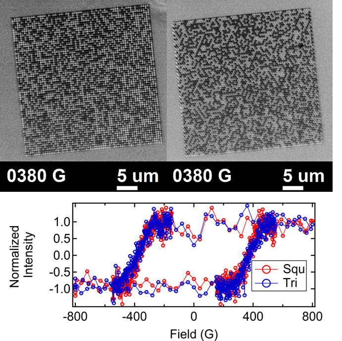
Figure 1: Top panel shows MOKE images recorded at 380 G in an increasing the field sweep, near the coercive field, for 500 nm lattice spacing square (left) and triangular (right) arrays from sample 2. The bottom panel shows normalized hysteresis loops recorded using imaging MOKE for these arrays with intensity averaged over the entire array area.

We begin with the run-to-run consistent, macroscopic (aggregate) aspects, starting with the switching field distribution and the contribution of island interactions thereto. The total field experienced by an island comprises not just the externally applied field $H_{\text{app}}$, but also a configuration-dependent contribution from other islands which broadens the distribution of observed (raw) switching fields. Without knowledge of the microstates the semi-empirical equation(Fraleigh et al., 2017)

$$\sigma=AKB_{0}(L)+\sigma_{d}$$ (1)

allows the observed width of the switching field distribution to be separated into contributions of island interactions and static disorder, the latter presumably introduced by the lithography process. Here, $A$ is a constant, $K$ an effective coordination number, $B_{0}(L)$ the dipolar field of an island on its nearest neighbor at lattice spacing $L$, and $\sigma_{d}$ the static disorder. Additionally, provided the microhistory, we can directly calculate the $r$-neighborhood-corrected switching field $h_{i,r}=H_{\text{app}}+$ (field from up-to-$r$^th neighbors) in point-dipole approximation, accounting for both the internal and external fields felt by an island when it switches. In this enriched notation, the raw switching field for sweep $\alpha$ is denoted as $h_{i,0}^{\alpha}$.

The top panel of Fig. 2 shows the distributions of the $r$-neighborhood-corrected switching fields $h_{*,r}^{\alpha}$ for a single sweep for a 500 nm square array from sample 2 for $0\leq r\leq 5$. These are the distributions of all aggregated islands, hence the ‘$*$’ subscript on $h$. The expected narrowing of the distribution as $r$ increases (further-neighbor fields accounted for) is prominent. The lower panels of Fig. 2 show how the widths of the $h_{*,r}^{\alpha}$ distributions change with lattice spacing for different lattice types. The broadening in the raw ($h_{*,0}^{\alpha}$) distributions for different geometries is accounted for completely by the difference in effective coordination number. For each geometry, as r is increased, the width decreases, becomes independent of the lattice spacing, and approaches the calculated value of disorder. The magnitude of the decrease is on the order of of $AKB_{0}(L)$, with K calculated considering $r$ neighbors. This decrease agrees with Eq. (1) and reduces to the static disorder contribution alone in the limit of large $r$. This behavior agrees with previous studies pointing to the significance of long-range interactions to the behavior of artificial spin ice(Chioar et al., 2014). The results in Fig. 2 were taken from sample 2; similar results are obtained for sample 3. The analysis supports the treatment of islands as interacting point dipoles, wherein an island’s neighbors influence its switching behavior by supplementing the external field with their net dipolar field strength.

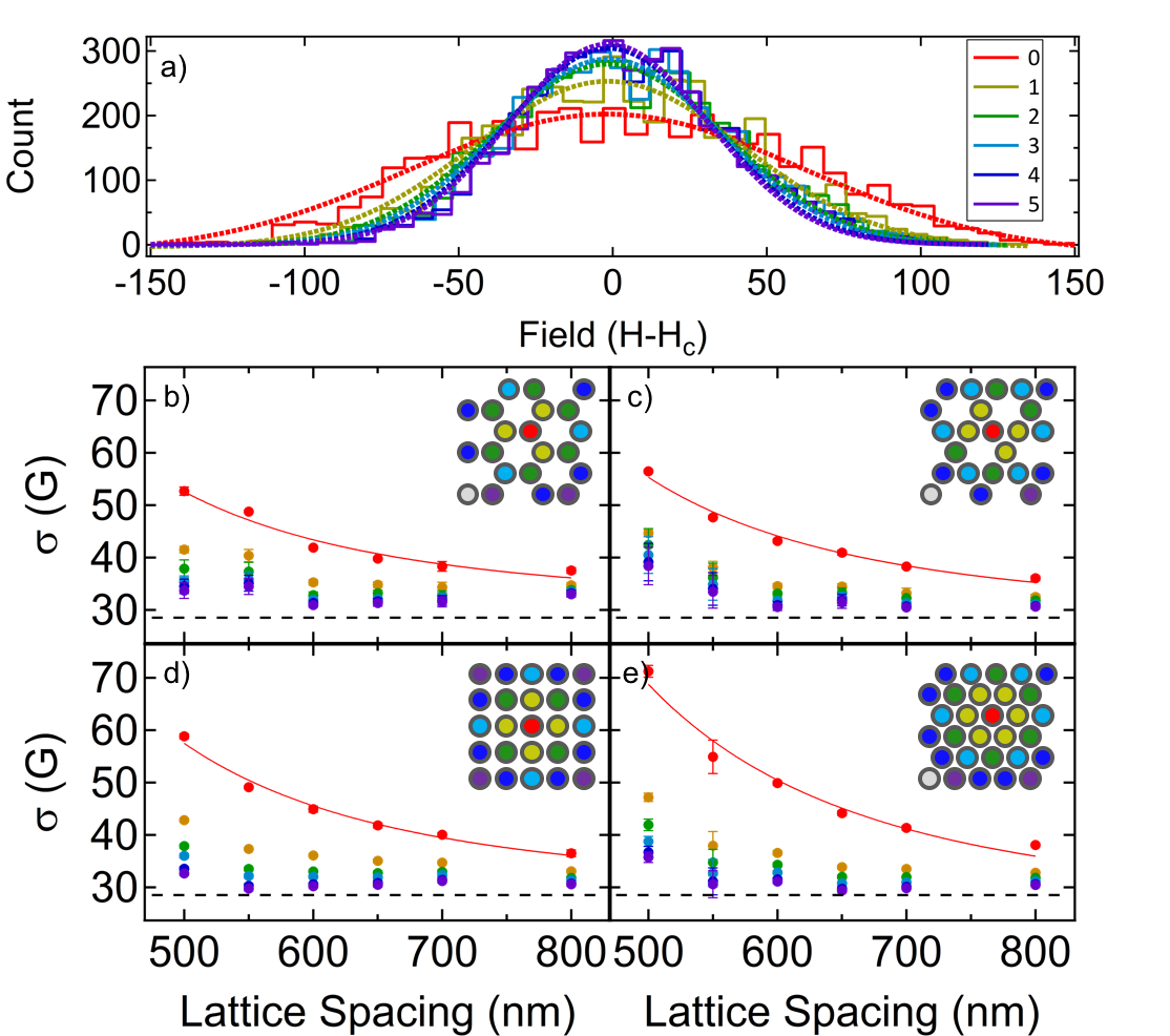
Figure 2: a) Switching field distribution and associated Gaussian fits, with switching fields calculated by removing dipolar effects from 0 (as measured) to 5 nearest neighbors for a 500 nm square array (Sample 2). Width of the Gaussian fits for b) hexagonal, c) kagome, d) square, and e) triangular as a function of lattice spacing taking into account increasing numbers of neighbors. Fits to Eq 1 are shown as red lines, and disorder values from these fits are shown as black dashed lines. The inset images show a cartoon of the lattice geometry colored by target island (red) and neighbor number to match the colors on the graphs. A full set of neighbors is shown up to third nearest neighbor, along with a partial set of fourth and fifth nearest neighbors.

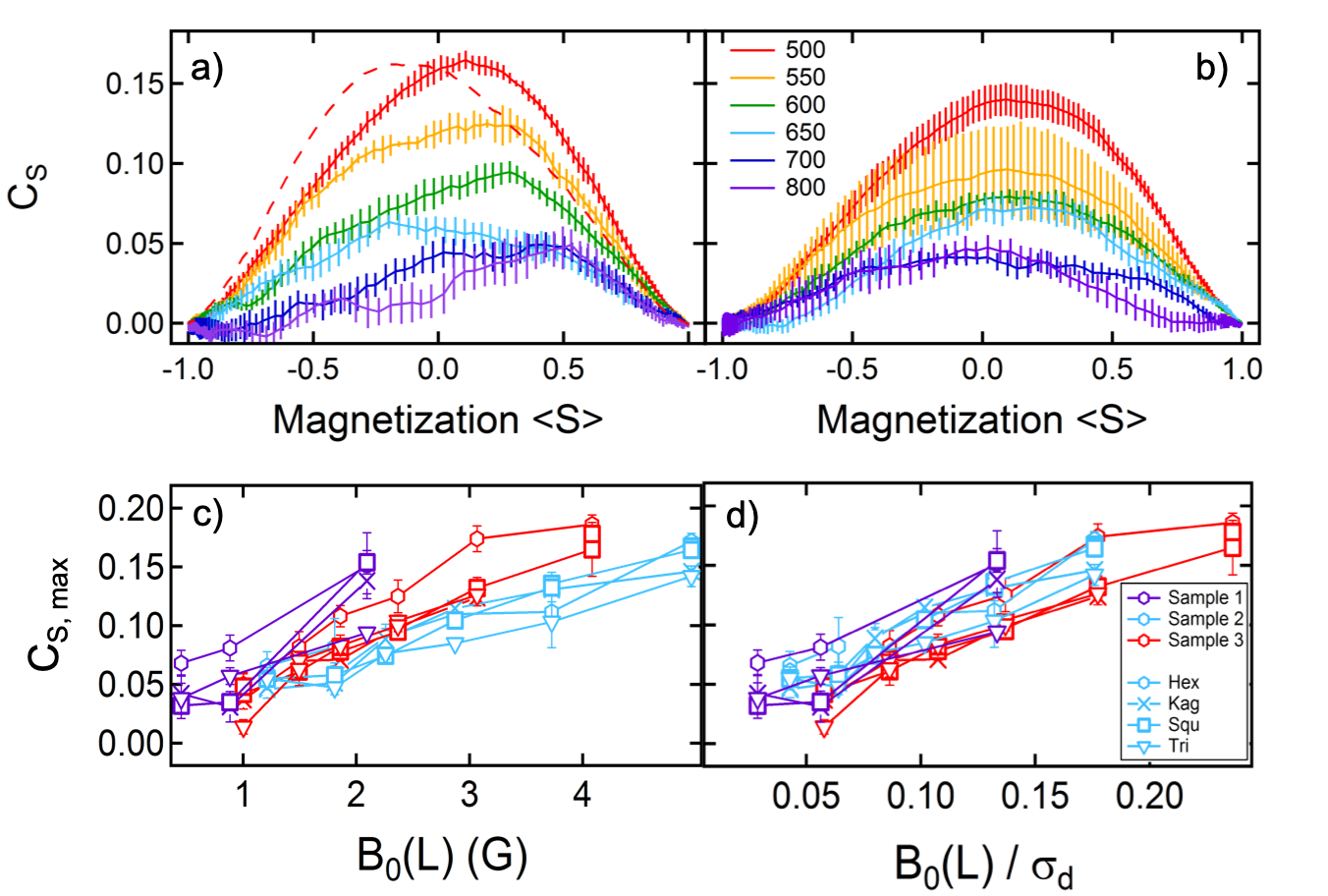
Figure 3: Plots of $C_{S}(\langle S\rangle$) for various lattice spacings of a) square, and b) triangular arrays from sample 2, for increasing values of applied field. The dashed line in panel a shows $C_{S}(\langle S\rangle)$ as the field is decreased to more clearly illustrate the asymmetry. Panel c) shows the maximum value of correlation as a function of the dipolar field of an island on its nearest neighbor (i.e. the interaction strength) for samples 1, 2, and 3. Panel d) shows the same data as a function of the dipolar field scaled by the measured disorder in the system.

While the $r$-neighborhood-corrected switching field distributions demonstrate an influence of islands on one another, they say nothing quantitative about correlations. We turn to these next. The average spin (magnetization) in an array during sweep $\alpha$ is $\langle S_{i}^{\alpha}\rangle_{i}$. Subscripts on averaging brackets indicate what is averaged over, and each spin takes value $+1$ or $-1$. $\langle S\rangle$ is a fairly reproducible function of external field (for the same sweep direction). For purposes of comparing different sweeps and different arrays, it is preferable to parametrize the macrohistory by magnetization $\langle S\rangle$ rather than the applied field; this will remove fluctuations due to finite size. Thus, the nearest-neighbor spin correlation for sweep $\alpha$,

$$C_{S}^{\alpha}(\langle S\rangle) =\Big{\langle}S_{i}^{\alpha}\Big{\rangle}_{i}\Big{\langle}S_{j}^{\alpha}\Big{\rangle}_{j}-\Big{\langle}S_{i}^{\alpha}S_{j}^{\alpha}\Big{\rangle}_{\alpha;\text{NN}}$$

$$=\langle S\rangle^{2}-\langle S_{i}^{\alpha}S_{j}^{\alpha}\rangle_{\text{NN}}$$ (2)

is regarded as a function of $\langle S\rangle$. The sum is over all nearest neighbor pairs $(i,j)$ as indicated briefly by the NN subscript. $C_{S}$ is zero if spins are independently assigned values $+1$ or $-1$ with probabilities consistent with $\langle S\rangle$, and we have chosen a sign convention such that it increases with the proportion of energetically preferred antiferromagnetic nearest-neighbor configurations. Fig. 3a,b show the evolution of $C_{S}^{\alpha}(\langle S\rangle)$ for up-sweeps for the square and triangular arrays on sample 2. The correlation increases and then decreases as the sample transitions from a saturated state, through zero magnetization to the oppositely saturated state. However, the correlation does not peak at zero magnetization. Rather, it continues to increase for a while, peaking at an offset $\langle S\rangle$. This behavior indicates the importance of the quasi-dynamic switching path and the influence of island interactions on it. While the offsets are repeatable and observed in multiple samples, the data are too noisy to discern any clear trends in the values.

One anticipates that the maximum value of nearest-neighbor antiferromagnetic correlation will increase with the strength of interactions, $B_{0}(L)$. Fig 3c shows that this expectation is borne out and that the dependence is roughly linear. Data for samples 1, 2, and 3 are plotted in different colors. For each sample, the maximum value of $C_{S}(\langle S\rangle)$ is consistent among all geometries, indicating that the interactions are not sufficiently strong for the distinction between frustrated and unfrustrated geometry to manifest in the macrostate. However, there is distinct variation in the correlations between samples, indicating that interaction strength is an insufficient parameter to characterize these systems. Using instead the dimensionless ratio $B_{0}(L)/\sigma_{d}$ of interaction strength to static disorder as independent variable, a significant, albeit partial, data collapse is obtained, as shown in Fig. 3d. Quite reasonably, local ordering is enhanced by increasing interaction strength and hampered by increasing static disorder.

Data and analyses discussed to this point show that the systems are macroscopically determinate, in that the histories of the global quantities $\langle S\rangle$ and $C_{S}$, as well as distributions of switching fields $h_{i,0}$ and $h_{i,r}$, are very similar run-to-run. A perfectly deterministic system, though, would have a reproducible microhistory, following exactly the same sequence of island switchings each time it is subjected to the same external field sweep. Possibly the simplest quantification of nonreproducibility is the run-to-run switching field variance

$$\sigma_{h}^{2}=\Big{\langle}\Big{(}h_{i}^{\alpha}-\overline{h_{i}}\Big{)}^{2}\Big{\rangle}_{i,\alpha},$$ (3)

where

$$\overline{h_{i}}=\langle{h_{i}^{\beta}}\rangle_{\beta}$$ (4)

is the run-averaged switching field of island $i$. The average in Eq. (3) is over islands in the array and multiple (7 – 10) macroscopically identical hysteresis loops. In contrast to the aggregate switching field distributions displayed in Fig. 2, the run-to-run variance inherently involves an average over runs and involves subtraction of an island-dependent mean. Table 1 reports average values across all geometries of the run-to-run switching field standard deviation (the square root of the variance) $\sigma_{h}$ for samples 2 and 3 at lattice spacings above 650 nm, of around 10 G. The standard deviation increases with increasing interaction strength, maximizing at around 20 G for the arrays with the strongest interaction. These values are much less than the width of the aggregate switching field distribution because they are measuring different quantities. The aggregate switching field distribution measures the variation of $h_{i}$ throughout a lattice, while these values measure the variation of individual island’s switching field around it’s mean value over a series of distinct runs.

Island switching is significantly influenced by local environment; this is already clear from the switching field distributions in Fig. 2. An indication of how this influence contributes to microhistory variation is provided by the switching field covariance

$$C_{h}=\Big{\langle}(h_{i}^{\alpha}-\overline{h_{i}})(h_{j}^{\alpha}-\overline{h_{j}})\Big{\rangle}_{\alpha;\text{NN}}.$$ (5)

This quantity is plotted for all arrays in Fig. 4a as a function of interaction strength $B_{0}(L)$. That $C_{h}$ is negative conforms to expectations since if one island switches “early”, it will increase the energy barrier for a neighbor to switch, due to the antiferromagnetic interactions. The arrays with the weakest interaction, although they show significant $\sigma_{h}$ (Table 1), show no significant covariance. As the interactions are increased, the covariance between neighboring island’s switching fields increase in magnitude. The increase in covariance also increases as a function of effective coordination number, similar to how the switching field distribution broadens with effective coordination number. In fact, at these interaction strengths, the impact of array geometry can be described completely by the coordination of the array, rather than whether or not there is frustration. The behavior at low interaction strength gives an indication of the intrinsic behavior of the islands, and the change with increasing interaction strength allows us to judge the impact of interactions. Because dynamics play a large role in the correlations of these systems, and there is some level of random variation that propagates through the lattice by neighbor interactions, it is likely that we will observe significant differences in the microstates.

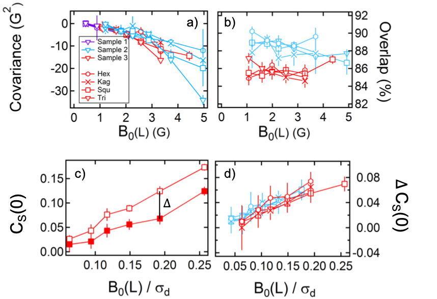
Figure 4: a) The covariance of switching fields between multiple runs for all three samples. b) The average overlap at the coercive field between pairs of runs for samples 2 and 3. Overlap is defined as the percent of islands which are in the same state in both states considered. c) The experimentally measured value of $C_{S}(0)$ (open squares) and the average value of $C_{S}(0)$ for randomly generated states with the experimentally measured overlap with the experimental state (solid squares), for a 500 nm square array from sample 3. The difference between these two curves is defined to be $\Delta C_{S}(0)$ d) The average difference in correlation between the experimentally measured state and a state with the experimentally measured average overlap.

To further characterize (non)reproducibility of the microhistory, we examine the average overlap

$$\overline{f_{=}}=\frac{1}{2}\left[1+\left\langle S_{i}^{\alpha}S_{i}^{\beta}\right\rangle_{i;\alpha\neq\beta}\right]$$ (6)

at zero magnetization, $\langle S\rangle=0$. The average overlap is simply the fraction of islands which are in the same state in a randomly chosen pair of distinct runs. Calculated values for samples 2 and 3 are plotted in Fig. 4b and range from 84% to 90%. Sample 2 has a consistently larger overlap than sample 3, which is reasonable since $\sigma_{h}$ is similar for the two samples while $\sigma_{d}$ is larger for sample 2. A larger ratio of $\sigma_{d}/\sigma_{h}$ implies that each island has access to a smaller subset of the switching region, increasing the number of islands in the same state at any given point in the switching process.

One may wonder whether an average overlap approaching 90% is enough by itself to explain the observed macrohistory repeatability. A simple numerical experiment shows this is not the case. Starting from one specific $\langle S\rangle=0$ microstate, we randomly select a fraction $1-\overline{f_{=}}$ of islands, flip them, and calculate the change $\Delta C_{S}(0)$ of the nearest-neighbor correlation (see Fig. 4c). Average values of $\Delta C_{S}(0)$ for 1000 repetitions of this experiment are plotted in Fig. 4d. The drop in $C_{S}$ is significantly greater than the standard deviation of the distribution over runs, hence one concludes that there is more to the correlations than simply the overlap. Indeed, one may calculate that if microstate $S^{\prime}_{i}$ is obtained from $S_{i}$ by independently flipping spins with prbability $1-\overline{f_{=}}$, that the nearest-neighbor correlation of the new microstate has an expectation value

$$\langle S^{\prime}_{i}S^{\prime}_{j}\rangle_{\text{NN}}=(1-2\overline{f_{=}})^{2}\langle S_{i}S_{j}\rangle_{\text{NN}}.$$ (7)

The origin(s) of microhistory stochasticity are not clear. Noise arising from the experimental setup, for instance in the power supply or magnet, seem unlikely to be responsible since such influences would be uniform across the sample; the magnetic field is quite homogeneous over our small field of view. However, the significant run-to-run switching field covariance shows that the stochasticity is at least strongly affected by local conditions. Prima facie, one expects thermal fluctuations to be completely negligible; the energy scale of room temperature $k_{B}T$ equals the magnetic energy of an island in a field of order $10^{-1}$ G, about 5% the field step size, which should lead to a high thermal stability at room temperature. However, near the coercive field, thermal fluctuations can be surprisingly significant in understanding the behavior of nanomagnetic systems.Braun (1993); Telepinsky et al. (2016) A non-negligible fraction of islands might be caused to switch in a slightly different field by a thermal fluctuation in a given run, and the “misstep” would then be amplified and propagated by island interactions. One might expect these propagated missteps to lead to a decrease in the zero magnetization overlap as the interactions are increased. However, we observe that the overlap is insensitive to interactions. This is possibly because only a subset of islands may be susceptible to thermal fluctuations at any given field step. Any island with a coercivity that is not sufficiently close to a given field is constrained to remain stable in its moment orientation at that field in all runs.

In conclusion, MOKE microscopy allows us to measure complete microhistories of perpendicular artificial spin ice. This level of detail allows a more direct and precise quantification of island interactions on macrohistory, as for instance in the $r$-neighborhood-corrected switching field distributions studied here. Perhaps more importantly, it allows precise determination of the degree of microhistory stochasticity. Our results suggest further studies to examine the mechanisms of microhistory stochasticity and fabrication of systems with interactions strong enough that frustration effects can be observed. In particular, a study of the impact of thermal fluctuations as a possible source for the stochastic behavior will open the possible inclusion of thermally-induced behavior in a broader range of magnetic systems.