Solving Differential Equation with Constrained Multilayer Feedforward Network

Abstract

In this paper, we present a novel framework to solve differential equations based on multilayer feedforward network. Previous works indicate that solvers based on neural network have low accuracy due to that the boundary conditions are not satisfied accurately. The boundary condition is now inserted directly into the model as boundary term, and the model is a combination of a boundary term and a multilayer feedforward network with its weight function. As the boundary condition becomes predefined constraintion in the model itself, the neural network is trained as an unconstrained optimization problem. This leads to both ease of training and high accuracy. Due to universal convergency of multilayer feedforward networks, the new method is a general approach in solving different types of differential equations. Numerical examples solving ODEs and PDEs with Dirichlet boundary condition are presented and discussed.

1 Introduction

Differential equations, including ordinary differential equations (ODEs) and partial differential equations (PDEs), are key mathematical models for various physics and engineering applications. In most situations, it is impractical to find analytical solutions, and numerical solutions become increasingly popular for these problems. When solving ODE/PDEs, one seeks for a function satisfying both (1) the differential equations within the domain, and (2) all initial/boundary conditions. Common numerical methods for ODEs are Runge-Kutta methods, linear multistep methods, and predictor-corrector methods [1]. As for PDEs, tremendous methods for discretizing the physical space or spectral space are developed, and the most common choices are finite difference method (FDM), finite volume method (FVM), finite element method (FEM), and spectral method. These methods are special cases of weighted residual method. Galerkin method is another numerical method based on weighted residual method for converting a continuous operator to a discrete form. It applies the method of variation of parameters to a function space and converts the original equation to a weak formulation.

In the present study, we take advantage of the fast developing machine learning technique and propose a framework of solving ODE/PDE by applying the variation of parameters of a neural network [2, 3]. Neural network (NN) is inspired by the complex biological neural network, and is now a computing system wildly applied in machine learning [4, 5, 6]. Feedforward network with full connection between neighboring layers is one of the first models introduced [7, 8], and the algorithms evaluating and training them have been studied since then [8, 9, 10, 11]. Besides applications in image recognition [5], natural language processing [6], cognitive science [12], and genomics [13], neural network is also a powerful tool for function approximation [14, 15, 16, 17, 18]. It is proved that functions in the form of multilayer feedforward network (MFN) is dense in function spaces such as $C(I)$ and $L^{2}(I)$ ($I$ is unit cube). It is also easily shown that increasing the layers of MFN will enormously increase its function approximation capability. However, deep neural networks are difficult to train with gradient methods such as backpropagation due to gradient vanishing [19, 20]. Here four-layer feedforward networks are chosen to avoid using special techniques such as ResNet [21].

Due to the ability of NN in function approximation, lots of efforts have been made to construct ODE/PDE solvers based on NN [22, 23, 2]. One of the major difficulties in such solvers is how to train a particular NN to satisfy the boundary condition accurately, since that the original form of NN as a trial function does not match boundary condition like trial functions in Galerkin methods. One strategy is the penalty method [2, 18, 24]. The penalty method has been applied successfully in Burgers equation [2], Laplace equation [18], and diffusion equations [24], but only limited accuracy can be achieved. Another issue is how to evaluate the derivatives in equations, which need to be compatible with the NN-based solver. One option is the so-called automatic differentiation (AD) [2]. AD evaluates the derivative with respect to input variable of any function defined by a computer program, and it is done by performing a non-standard interpretation of the program: the interpretation replaces the domain of the variables and redefines the semantic of the operators [25].

In our framework, we define a trial function which consists of a bulk term and a boundary term. The boundary term matches initial/boundary conditions, and the bulk term satisfies a reduced problem with relaxed boundary constrains, respectively. The boundary term can be construct explicitly. We then define for the bulk term a loss function, which is actually the residual of the reduced problem. Such loss function does not involve any boundary conditions since the boundary conditions are relaxed in the reduced problem. Finally the bulk term, and therefore the trial function, is determined by minimizing the loss function. Machine learning technique is used for this minimization of the loss function. We refer to this new strategy as the constrained multilayer feedforward network (CMFN) method. With such novel strategy we will show that much higher accuracy can be achieve. It should also be pointed out that any method can be used to minimizing the loss function.

Before proceeding, we would like to clarify some terminology. In the language of the machine learning community, the trial function is usually called model. The minimization of the loss function is actually a learning process, during which the trial function learns the correct data distribution of analytical solution. The minimization process is also a standard optimization problem, and it is equivalent to training in machine learning. Thus, the terminologies “training”, “optimization”, and “minimization” will be used interchangeably throughout this paper.

The paper is organized as follows. In section 2 we describe the framework in detail. Section 3 presents some numerical examples. Finally section 4 concludes the paper.

2 Numerical Method

To solve ODEs/PDEs numerically, one finds a function which satisfies the differential equations inside the domain and all initial/boundary conditions at (temporal/spatial) boundaries. That is, two parts of information need to be transferred into the numerical solver. For instance, in FVM the former part of information is transferred by flux reconstruction and the later part by operations on the boundary cells, respectively. In CMFN method, the former part of information is transferred by directly applying the differential operators with AD technique. The initial/boundary conditions are dealt with the boundary term in the trial function.

The CMFN method is based on the concept of MFN. MFN with $n$ layers can be defined as a computing algorithm as follows. The input layer as a vector is denoted by $y^{(1)}$, the output layer is denoted by $y^{(n)}$, and the hidden layers by $y^{(i)}$. The output layer $y^{(n)}$ is computed by hidden layer $y^{(n-1)}$:

$$y^{(n)}_{k}=\sum_{j}\theta^{(n-1)}_{kj}y^{(n-1)}_{j}+\beta_{k}^{(n-1)},$$

and the hidden layers are computed recursively by:

$$\begin{cases}z^{(i+1)}_{k}=\sum_{j}\theta^{(i)}_{kj}y^{(i)}_{j}+\beta_{k}^{(i)}\\ y^{(i+1)}_{k}=\phi(z^{(i+1)}_{k})\end{cases}\quad i=1,2,\ldots,n-2.$$

Explicitly, a three-layer feedforward network $N(x;\theta,\beta)$ is defined with superposition of activation function $\phi$ over linear transformation ($x=\{x_{i}\}_{n\times 1}$ as input layer and $N(x;\theta,\beta)=\{N_{k}\}_{m\times 1}$ as output layer):

$$N_{k}=\sum_{j}\theta_{kj}^{(2)}\phi(\sum_{i}\theta_{ji}^{(1)}x_{i}+\beta_{j}^{(1)})+\beta_{k}^{(2)},$$ (1)

and a four-layer MFN is

$$N_{l}=\sum_{k}\theta_{lk}^{(3)}\phi(\sum_{j}\theta_{kj}^{(2)}\phi(\sum_{i}\theta_{ji}^{(1)}x_{i}+\beta_{j}^{(1)})+\beta_{k}^{(2)})+\beta_{l}^{(3)}.$$ (2)

The parameters of the MFN are its weights $\theta=\{\theta_{ij}^{(k)}\}$ and biases $\beta=\{\beta_{j}^{(k)}\}$. It has been proved that the MFN eq. 2 with proper activation $\phi$ is dense in $C(I)$, namely the set of all continuous functions defined on unit cube [15]. Therefore, for any continuous function $y(x)$ defined on a finite domain, one set of parameters $(\theta^{*},\beta^{*})$ can be found such that the corresponding network $N(x;\theta^{*},\beta^{*})$ is close enough to $y(x)$, i.e. the norm $\|y(x)-N(x;\theta^{*},\beta^{*})\|$ could be sufficiently small. Similar conclusion holds for $y\in L^{2}(I)$, which is $\int_{I}|y(x)|^{2}\differential{x}<\infty$. Such properties guarantee that an optimal set of $N(x;\theta^{*},\beta^{*})$ exists with the corresponding MFN being a good numerical approximation of the solution.

A well-posed ODE/PDE with Dirichlet boundary condition can be written as

$$\begin{cases}\mathcal{L}u=f&\mbox{\quad in\quad}\Omega,\\ \mathcal{B}u=g&\mbox{\quad in\quad}\partial\Omega.\end{cases}$$ (3)

In CMFN we define a model function:

$$\hat{y}(x;\theta,\beta)=G(x)+\tilde{N}(x;\theta,\beta)\equiv G(x)+w(x)\cdot N(x;\theta,\beta).$$ (4)

As the boundary operator $\mathcal{B}$ is linear and algebraic, we choose the two terms $G(x)$ and $w(x)$ in eq. 4 such that

1. $\mathcal{B}G=g$ when $x\in\partial\Omega$,

2. $\mathcal{B}\tilde{N}\to 0$ when $x\to\partial\Omega$.

$G(x)$ is a boundary term which is a pre-defined function, $\tilde{N}(x)$ is bulk term, and $N(x)$ is the unknown part which is approximated by a neural network. The original problem with respect to $u(x)$ in eq. 4 is reduced to solving a new differential equation with respect to $\tilde{N}(x)$. The the new equation is defined as the reduced equation, and the unknown part $N(x)$ separated from bulk term is called reduced solution.

In eq. 4, as long as a pre-defined weight $w(x)$ is a bounded continuous function, the bulk term $\tilde{N}(x)$ is continuous and bounded according to eq. 2. The bulk term is further written as $\tilde{N}(x)=w(x)\cdot N(x)$, where the pre-defined weight $w(x)$ satisfies:

1. $w(x)\to 0$ as $x\to\partial\Omega$ (vanishing on domain boundary),

2. for all $x^{*}\in\Omega$, $w(x^{*})\neq 0$ (non-vanishing within domain).

Now the boundary conditions are automatically satisfied, or we say, the boundary conditions are relaxed in the reduced equation. Once the reduced equation is determined, the loss function can be constructed without considering the original boundary conditions.

By substituting the trial function $\hat{y}(x)=G(x)+w(x)\cdot N(x)$ into eq. 3, the original problem is converted to its reduced equation:

$$\mathcal{L}[G+w\cdot N]=\tilde{\mathcal{L}}[N]=f\quad N\in C(\mathbb{R}^{n}).$$ (5)

One may think that there could be multiple solutions to reduced equation since it has no boundary conditions. However, while the original problem eq. 3 has unique solution $y^{*}$, the reduced one eq. 5 should also have a unique solution $(y^{*}-G)/w$. The paradox indicates that, among all solutions to eq. 5, there exists a unique solution satisfies: $\mathcal{B}\tilde{N}\to 0$ while $x\to\partial\Omega$. We do not have a rigorous proof for this statement yet, but as supported by the examples shown later, a unique solution can always be obtained.

After construction of trial function $\hat{y}$, the loss function towards which optimization is done is defined by residual $\mathcal{R}N=\tilde{\mathcal{L}}N-f$ of eq. 3:

$$L=\int_{\Omega}\left\langle(\mathcal{R}N)(x),(\mathcal{R}N)(x)\right\rangle\differential{x}=\sum_{x^{*}\in T(\Omega)}\|(\mathcal{R}N)(x^{*})\|^{2},$$ (6)

where $T(\Omega)$ is the training set containing points selected from domain $\Omega$. The operator $\mathcal{R}$ is defined by AD instead of manually working it out. This not only saves the researches from laborious job [23], but also produces robust and reliable code [26, 25]. There are successful AD implements on nearly all programming platforms [26]. In this work, reverse mode AD application programming interface on TensorFlow [27] is called. Since AD solves the problem of much too complicated differential problem, high order differential operator $\mathcal{L}$ are solved in this work without extra efforts.

The final stage of the framework solving ODE/PDE is optimization during which loss function $L$ defined by eq. 6 is minimized with respect to its free parameters. In cases where MFN $N(x;\theta,\beta)$ is the reduced solution, its weights and biases $(\theta,\beta)$ are trained to minimize $L=L(\theta,\beta)$. In this work, the optimization is done by second order method L-BFGS [28], instead of SGD, the most popular choice in building machine learning models [6]. The second order method is not always robust in general machine learning problems, but it serves well in ODE/PDE solver according to our observation. All numerical examples presented in later section in this paper is trained by second order method L-BFGS which greatly improves training efficiency. The training process requires large amount of computational resource which used to be an obstacle in development of machine learning [10]. Parallelism and heterogeneous computing throw lights on the problem, and the model in this work is defined and trained on TensorFlow [27].

3 Examples and Discussion

The first example on ODE solving is a definite integral problem as illustration:

$$\begin{cases}y^{\prime}(x)=\cos x\\ y(x=0)=y_{0}=1\end{cases}.$$ (7)

The analytical solution is simply integration of R.H.S. of eq. 7: $y(x)=1+\sin x$. In order to find a numerical solution in domain $[0,10]$. The trial function is defined as

$$\hat{y}(x;\theta,\beta)=y_{0}e^{-x}+(1-e^{-x})N(x;\theta,\beta).$$ (8)

It is easily verified that requirements for $G(x)$ and $\tilde{N}(x)$ are all satisfied. The network $N(x;\theta,\beta)$ is set as a four-layer network with $20$ neurons in each hidden layer. Loss function is defined as

$$L=\int_{0}^{10}\|\hat{y}^{\prime}-\cos x\|^{2}\differential{x}=\sum_{i=1}^{1000}|\hat{y}^{\prime}(x_{i})-\cos x_{i}|^{2},$$ (9)

with $\{x_{i}\}_{i=1,2,\ldots,1000}$ are uniformly selected in interval $[0,10]$. The loss function is minimized by L-BFGS method, the result is illustrated in fig. 1.

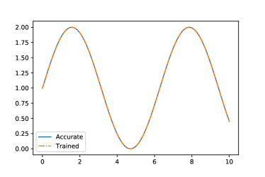
(a)

(b)

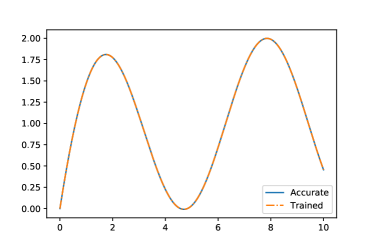
(c)

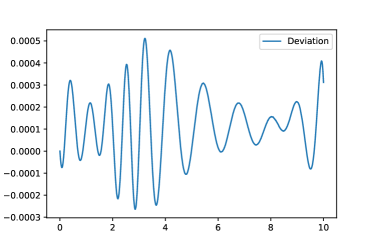
(d)

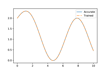
(e)

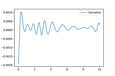
(f)

Figure 1: Results of definite integral problem in eq. 7 with $\mathrm{Error}=1.96\times 10^{-4}$

The boundary condition is well maintained in this example. LABEL:fig:1d-integral-y, LABEL:fig:1d-integral-core and LABEL:fig:1d-integral-N shows that the trained MFN provides a correct reduced solution, as well as a good match in bulk term and the whole model. However, error distributions shown in LABEL:fig:1d-integral-y-dev, LABEL:fig:1d-integral-core-dev and LABEL:fig:1d-integral-N-dev reveal that the reduced solution actually has the lowest accuracy, especially on domain boundary, the pre-defined constrains in $G(x)$ and $w(x)$ reduce error in model, as well as turn the training process into a standard non-constrained optimization problem.

Another important property shown in LABEL:fig:1d-integral-y-dev is that the solution learned by CMFN deviates from analytical solution randomly, where traditional numerical methods usually have increasing errors along iterations. This property is natural for CMFN method since all data points are equal to the learning process, while in iteration methods error grows accumulatively. A more accurate measure of error in solution provided by eq. 8 is calculating the $L^{2}$-norm of error distribution:

$$\mathrm{Error}=\sqrt{\frac{1}{10}\int_{0}^{10}|y(x)-\hat{y}(x)|^{2}\differential{x}.}$$ (10)

The previous example has an average error of $1.96\times 10^{-4}$. The authors also tried other choices on defining boundary term $G$ and weight function $w$: $G^{*}(x)\equiv 1$ and $w^{*}(x)=x$. Numerical test shows that definitions in eq. 8 is more optimized than their alternatives. $G^{*}(x)$ instead of original $G(x)$ in eq. 8 roughly doubles the average error, and $w^{*}(x)$ instead the original weight even reduces the accuracy for one order of magnitude.

As is mentioned above, the reduced equation with relaxed boundary condition should have unique solution instead of multiple solution under the premise that the solution is bounded. The reduced equation for eq. 7 is

$$(1-e^{-x})N^{\prime}+e^{-x}N-y_{0}e^{-x}-\cos x=0,$$ (11)

and the general solution to eq. 11 is

$$N(x)=\frac{C-y_{0}e^{-x}}{1-e^{-x}}+\frac{\sin x}{1-e^{-x}}\quad C\in\mathbb{R}.$$ (12)

At $x=1$, the first part in R.H.S. of eq. 12 is unbounded if $C\neq y_{0}$; if $N(x)$ is assumed to be a bounded function on $[0,1]$, then in eq. 12 there exists unique solution which is a proper reduced solution to problem in eq. 7.

The CMFN treats the problems defined by eq. 3 equally, so any initial condition problem is solved with similar process and accuracy. The following presents solution of boundary value problem (BVP) of a second order ODE. It is boundary layer problem [29] reduced to 1D:

$$uu^{\prime}=\nu u^{\prime\prime}\quad\quad u(0)=1\quad u(1)=0.$$ (13)

The problem has analytical solution:

$$u(x)=\frac{2C}{1+\exp\left(\frac{x-1}{\nu}\cdot C\right)}-C\quad C>1,$$ (14)

with $C$ as a constant determined by algebraic equation:

$$1-\frac{2}{1+C}=\exp\left(-\frac{C}{\nu}\right).$$

We have $C\approx 1.2$ when $\nu=0.5$, and $C$ tends to $1$ rapidly as $\nu$ decreases to $\nu=0$.

The boundary term of model is constructed according to boundary conditions in eq. 13 where linear function $f(x)=1-x$ is sufficient in matching values of the two boundary points. The weight function is constructed by polynomial such that $w(0)=0$ and $w(1)=0$. Finally, the trial function is defined as

$$\hat{u}(x;\theta,\beta)=(1-x)+x(1-x)\cdot N(x;\theta,\beta),$$ (15)

and loss function is defined similar to eq. 8. The model is trained with $100$ data points uniformly distributed in $[0,1]$.

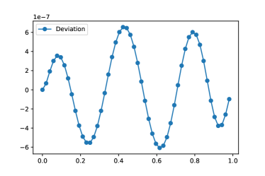
(a)

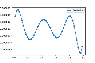
(b)

Figure 2: Error distributions of BVP with average error $<10^{-5}$

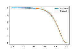
(a)

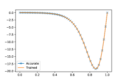
(b)

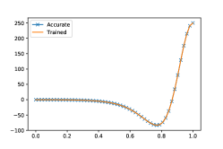
(c)

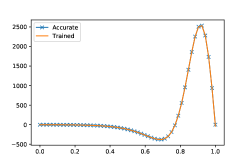
(d)

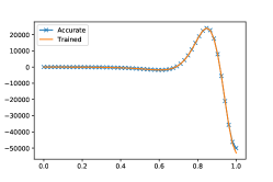
(e)

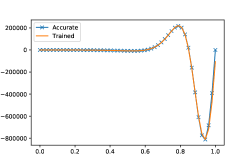
(f)

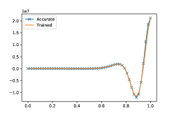
(g)

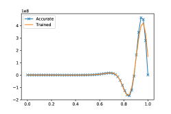
(h)

Figure 3: Differentiation of learned solution of eq. 13

Figure 2 shows that BVP is solved with high numerical accuracy, and in LABEL:fig:bl-diff1 to 3h differential property of the learned solution is studied. CMFN solution to the problem is not only an accurate numerical approximation to the analytical solution, but its first to eighth order derivatives are also all accurate numerical approximations to their analytical counterpart. This is very hard to achieve with commonly used numerical methods enumerated in section 1.

Another important observation is that once weight is defined by polynomials, there is a sole proper choice based on initial/boundary condition: for 1D Dirichlet boundary contion at $x=a$, there would be a factor $(x-a)$ in the weight function. For example, weight in eq. 15 should be defined as $w(x)=x(1-x)$, which is Hermite interpolation based on boundary condition: $w(1)=w(0)=0$; if weight is defined as $w^{*}(x)=x^{2}(1-x)$ instead, there will be a huge reduction in accuracy. Since the term $x^{2}$ in $w^{*}(x)$ not only vanishes itself at $x=0$, but also has zero first order derivative there; as a result, the boundary term $G(x)$ unexpectedly dominates both function value and first order derivative at $x=0$.

Two dimensional problem is tested with heat conduction problem (Laplace equation):

$$\nabla^{2}T(x,y)=0\quad\quad x\in[0,1]\quad y\in[0,1]$$ (16)

The boundary condition of Dirichlet problem is:

$$T(0,y)=T(1,y)=T(x,0)=0\quad T(x,1)=\sin\pi x.$$ (17)

The problem has analytical solution:

$$T(x,y)=\frac{\sin\pi x\sinh\pi y}{\sinh\pi},$$ (18)

so the error of numerical solution $\hat{T}(x,y)$ is evaluated as:

$$\mathrm{Error}=\sqrt{\frac{1}{S_{\Omega}}\int_{\Omega}|T(x,y)-\hat{T}(x,y)|^{2}\differential{\Omega}},$$ (19)

with $S_{\Omega}$ being area of domain ($S_{\Omega}=1$).

The model for Dirichlet problem is

$$\hat{T}(x;\theta,\beta)=y\sin\pi x+x(1-x)y(1-y)\cdot N(x;\theta,\beta).$$ (20)

It is easily verified that the requirements for $G$ and $\tilde{N}$ are satisfied. The weight function is actually constructed by the principle discussed above: it consists of factors from all four boundary conditions.

The loss function is constructed similar to eq. 9, and the simulation is done by a MFN with $2$ hidden layers and $40$ neurons in each hidden layer. The data points training the network is a set of $900$ items which are vertices of a $30\times 30$ uniform mesh on two dimensional unit cube. The results of simulation is demonstrated in fig. 4. LABEL:fig:heat-accurate is contour of analytical solution to eq. 18, and the simulated solution in LABEL:fig:heat-dirichlet matches the analytical solution quite exactly. LABEL:fig:heat-error illustrates the pointwise deviation from analytical solution of bulk term. The average error in LABEL:fig:heat-dirichlet is $2.8\times 10^{-6}$. The similar case calculated by penalty method reported in [2, 18] is only of order $10^{-3}$.

(a)

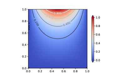
(b)

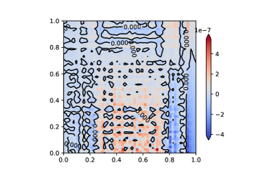
(c)

Figure 4: The results for simulating Laplace equation

The two properties distinguish CMFN from other methods are its generality and accuracy. As for the generality side, this framework is not sensitive to the property of differential equation; it works similarly on elliptic, hyperbolic, and parabolic problems. One interesting verification is that turning the original problem into a convection-diffusion problem:

$$u\frac{\partial T}{\partial x}+v\frac{\partial T}{\partial y}=\nabla^{2}T+f,$$ (21)

the boundary condition is set the same as in eq. 17, as a Dirichlet problem, and all other configurations such as network topology and training set are all the same as previous. The convection velocities $(u,v)$ and source term $f$ are assigned artificially as:

$$u(x,y)=y^{2}\cos x,$$

$$v(x,y)=\frac{1}{3}y^{3}\sin x,$$

$$f(x,y)=y^{2}\cos x\frac{\pi\cos\pi x\sinh\pi y}{\sinh\pi}+\frac{1}{3}y^{3}\sin x\frac{\pi\sin\pi x\cosh\pi y}{\sinh\pi}+$$

$$\alpha\left(2\pi^{2}\sin 2\pi x\cos 2\pi y-4\pi^{2}\sin 2\pi x\sin^{2}\pi y\right)-$$

$$\alpha\left(2\pi y^{2}\cos x\cos 2\pi x\sin^{2}\pi y+\frac{\pi}{3}y^{3}\sin x\sin 2\pi x\sin 2\pi y\right)$$

$$\alpha=0.1.$$

This setup ensures that the analytical solution is:

$$T(x,y)=\frac{\sin\pi x\sinh\pi y}{\sinh\pi}-\alpha\sin 2\pi x\sin^{2}\pi y$$ (22)

The simulated solution is shown in fig. 5, its average error is $8.57\times 10^{-4}$, while the elliptic counterpart of the problem has average error of $2.6\times 10^{-5}$.

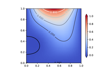
(a)

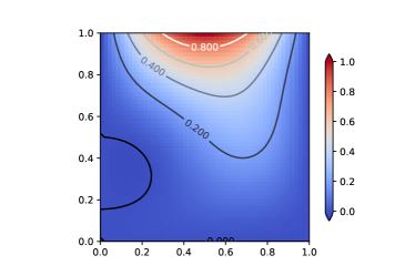
(b)

Figure 5: Convection-diffusion problem with average error of $8.57\times 10^{-4}$

Another important property of CMFN is its accuracy. While solving Laplace equation, penalty method such as PINN [18] is only able to achieve an average error of $1.6\times 10^{-3}$, and it is easily observed that boundary conditions are not accurately satisfied (especially in the two lower corners of fig. 6), but CMFN keeps the boundary conditions being satisfied accurately in an intrinsic way.

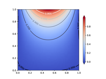
(a)

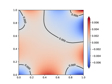
(b)

Figure 6: Numerical solution by PINN method with average error of $1.6\times 10^{-3}$

4 Conclusion and Future Work

In this paper, we present a novel framework of constructing ODE/PDE solver based on CMFN method. The numerical method and its application are discussed with regard to ODEs and PDEs with Dirichlet boundary conditions.

CMFN method stands out for its generality and accuracy. Traditional neural network methods based on RBF [30] or penalty methods [2] have very limited accuracy. By constructing the trial function with a weighted reduced solution as bulk term and a pre-defined boundary term, the model satisfies the boundary condition automatically, and as a result, the training based on residuals of differential equations could be more effective. Moreover, the CMFN method trains the neural network with all input data simultaneously, so it is intrinsically able to remain accuracy in numerically solving the differential equation on large domain and large time span. The iteration methods such as FVM and FDM accumulate truncation error in each step, so the scheme has to be designed carefully to be applied to larger domain and larger time span, while methods based on neural network does not has the obsession.

The generality of CMFN framework is in several aspects. The iteration methods such as FDM, FVM, and FEM are sensitive to property of PDE, since the growth of numerical error differs in hyperbolic, parabolic, and elliptic problems. CMFN instead provides a unified method. Compared with traditional neural network methods based on RBF [30], CMFN can be applied similarly on both linear and nonlinear problems while the later usually only works on linear problem. In this work, very simple network topology (four-layer feedforward network with twenty neurons) and very small data (less than $10^{3}$ points) are used, but heat transfer equation and convection-diffusion equation with Dirichlet boundary condition on unit cube are solved successfully on the same model.

Another property of CMFN method being worth mentioning is the indeterminacy in numerical result. In the training stage of our new framework, there is an initial guess on MFN. Since the network has tremendous parameters, it has to be randomly initialized; after training, the loss function would be reduced to a small number, but usually not zero, so the optimal solution is not usually obtained. The above two factors lead to the result that each specific parameter of MFN has rather random behavior. However the overall behavior of the computational machine is controllable, because as long as the object function has enough continuity, the error would reduce along with reduction of loss function.

This work is a new starting point in the field of constructing PDE solver for the authors. There are several works could be considered in the future:

1. finding a general method to construct proper form of bulk term for Neumann boundary condition;

2. finding a systematical method of constructing weight and boundary term, especially for complex geometry;

3. building larger and deeper networks for more complex problems such as Navier-Stokes equation; and

4. giving out a more mathematically rigorous proof on existence and uniqueness of reduced solution.

References

- [1] Richard L Burden and J Douglas Faires. Numerical analysis. 2001. Brooks/Cole, USA, 2001.
- [2] Maziar Raissi, Paris Perdikaris, and George Em Karniadakis. Physics informed deep learning (part i): Data-driven solutions of nonlinear partial differential equations. arXiv preprint arXiv:1711.10561, 2017.
- [3] Isaac E Lagaris, Aristidis Likas, and Dimitrios I Fotiadis. Artificial neural networks for solving ordinary and partial differential equations. IEEE transactions on neural networks, 9(5):987–1000, 1998.
- [4] Simon S Haykin. Neural networks and learning machines, third edition. Pearson Education, Inc., 2009.
- [5] Alex Krizhevsky, Ilya Sutskever, and Geoffrey E Hinton. Imagenet classification with deep convolutional neural networks. In Advances in neural information processing systems, pages 1097–1105, 2012.
- [6] Yann LeCun, Yoshua Bengio, and Geoffrey Hinton. Deep learning. nature, 521(7553):436, 2015.
- [7] Warren S McCulloch and Walter Pitts. A logical calculus of the ideas immanent in nervous activity. The bulletin of mathematical biophysics, 5(4):115–133, 1943.
- [8] Frank Rosenblatt. The perceptron: a probabilistic model for information storage and organization in the brain. Psychological review, 65(6):386, 1958.
- [9] Frank Rosenblatt. Principles of neurodynamics. Spartan Book, 1962.
- [10] Marvin Minsky and Seymour A Papert. Perceptrons: an introduction to computational geometry. MIT press, 1969.
- [11] Paul Werbos. Beyond regression: new tools for prediction and analysis in the behavioral sciences. PhD thesis, Harvard University, 1974.
- [12] Brenden M Lake, Ruslan Salakhutdinov, and Joshua B Tenenbaum. Human-level concept learning through probabilistic program induction. Science, 350(6266):1332–1338, 2015.
- [13] Babak Alipanahi, Andrew Delong, Matthew T Weirauch, and Brendan J Frey. Predicting the sequence specificities of dna-and rna-binding proteins by deep learning. Nature biotechnology, 33(8):831, 2015.
- [14] Kurt Hornik, Maxwell Stinchcombe, and Halbert White. Multilayer feedforward networks are universal approximators. Neural networks, 2(5):359–366, 1989.
- [15] George Cybenko. Approximation by superpositions of a sigmoidal function. Mathematics of control, signals and systems, 2(4):303–314, 1989.
- [16] Lee K Jones. Constructive approximations for neural networks by sigmoidal functions. Proceedings of the IEEE, 78(10):1586–1589, 1990.
- [17] S Carroll and B Dickinson. Construction of neural networks using the radon transform. In IEEE International Conference on Neural Networks, volume 1, pages 607–611. IEEE, 1989.
- [18] Zeyu Liu, Yantao Yang, and Qingdong Cai. Neural network as a function approximator and its application in solving differential equations. Applied Mathematics and Mechanics, 40(2):237–248, 2019.
- [19] S Hochreiter. Untersuchungen zu dynamischen neuronalen netzen [in german]. Diploma thesis, TU Münich, 1991.
- [20] Sepp Hochreiter, Yoshua Bengio, Paolo Frasconi, Jürgen Schmidhuber, et al. Gradient flow in recurrent nets: the difficulty of learning long-term dependencies, 2001.
- [21] Kaiming He, Xiangyu Zhang, Shaoqing Ren, and Jian Sun. Deep residual learning for image recognition. In Proceedings of the IEEE conference on computer vision and pattern recognition, pages 770–778, 2016.
- [22] Susmita Mall and Snehashish Chakraverty. Chebyshev neural network based model for solving lane–emden type equations. Applied Mathematics and Computation, 247:100–114, 2014.
- [23] Jens Berg and Kaj Nyström. A unified deep artificial neural network approach to partial differential equations in complex geometries. arXiv preprint arXiv:1711.06464, 2017.
- [24] Qianshi Wei, Ying Jiang, and Jeff ZY Chen. Machine-learning solver for modified diffusion equations. Physical Review E, 98(5):053304, 2018.
- [25] Louis B Rall. Automatic differentiation: Techniques and applications. Springer, 1981.
- [26] Atilim Gunes Baydin, Barak A Pearlmutter, Alexey Andreyevich Radul, and Jeffrey Mark Siskind. Automatic differentiation in machine learning: a survey. arXiv preprint arXiv:1502.05767, 2015.
- [27] Martín Abadi, Ashish Agarwal, Paul Barham, Eugene Brevdo, Zhifeng Chen, Craig Citro, Greg S. Corrado, Andy Davis, Jeffrey Dean, Matthieu Devin, Sanjay Ghemawat, Ian Goodfellow, Andrew Harp, Geoffrey Irving, Michael Isard, Yangqing Jia, Rafal Jozefowicz, Lukasz Kaiser, Manjunath Kudlur, Josh Levenberg, Dandelion Mané, Rajat Monga, Sherry Moore, Derek Murray, Chris Olah, Mike Schuster, Jonathon Shlens, Benoit Steiner, Ilya Sutskever, Kunal Talwar, Paul Tucker, Vincent Vanhoucke, Vijay Vasudevan, Fernanda Viégas, Oriol Vinyals, Pete Warden, Martin Wattenberg, Martin Wicke, Yuan Yu, and Xiaoqiang Zheng. TensorFlow: Large-scale machine learning on heterogeneous systems, 2015. Software available from tensorflow.org.
- [28] Dong C. Liu and Jorge Nocedal. On the limited memory bfgs method for large scale optimization. Mathematical Programming, 45(1):503–528, Aug 1989.
- [29] L Prandtl. Zur berechnung der grenzschichten. Zamm-zeitschrift Fur Angewandte Mathematik Und Mechanik, 18(1):77–82, 1938.
- [30] Nam Mai-Duy and Thanh Tran-Cong. Numerical solution of differential equations using multiquadric radial basis function networks. Neural networks, 14(2):185–199, 2001.