Simple Parking Strategies

Abstract

We investigate simple strategies that embody the decisions that one faces when trying to park near a popular destination. Should one park far from the target (destination), where finding a spot is easy, but then be faced with a long walk, or should one attempt to look for a desirable spot close to the target, where spots may be hard to find? We study an idealized parking process on a one-dimensional geometry where the desired target is located at $x=0$, cars enter the system from the right at a rate $\lambda$ and each car leaves at a unit rate. We analyze three parking strategies—meek, prudent, and optimistic—and determine which is optimal.

1 Introduction

When driving to a popular destination, nearby parking spots are hard to find. Where should one park? Should one park far from the destination, or target, where spaces are likely to be plentiful and then walk a long way to the target? Alternatively, should one be optimistic and drive close to the target and look only for nearby parking? If one uses the latter strategy, it is possible that there are no nearby parking spots and then one has to backtrack to find a more distant parking spot, thereby wasting time.

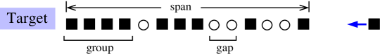
Figure 1: Parking in a one-dimensional lot where cars (squares) enter from the right. Circles represent empty spots, and empty spots to the right of the furthest car are not shown. The spatial range of the parked cars is defined as the span.

As one might anticipate, this practical problem has been the focus of considerable study in the transportation engineering literature (see, e.g., [1, 2, 3, 4, 5, 6, 7] and references therein). These practically minded studies include many real-world effects, such as parking costs, parking limits, and urban planning implications, that cannot be accounted for in minimalist physics-based modeling. In the context of granular compaction, the “parking lot model” describes how a finite interval with input and output of cars progressively densifies due to various compaction mechanisms [8, 9, 10, 11, 12, 13, 14]. In this work, we explore simple parking strategies in an idealized one-dimensional geometry and determine their relative advantages.

In our modeling, we assume that cars enter the system from the right at a fixed rate $\lambda$ and park at integer points along a one-dimensional semi-infinite line, which plays the role of a parking lot. Cars also independently leave the lot at a unit rate. For a lot that contains $N$ parked cars, the total car departure rate therefore equals $N$. The first car that enters will park at $x=1$, the closest spot to the target. The second car will park at $x=2$ if the first car has not left at the moment when the second car arrives. We assume that all cars have the same size and fill exactly one parking spot. As the parking lot fills, the parked cars forms contiguous groups that are interspersed with gaps (Fig. 1). The most interesting situation is $\lambda\gg 1$, so that the number of parked cars is large. We also assume that when a car enters the lot, it has time to find a parking space before the next car enters.

In the steady state, the number of parked cars is a random quantity that fluctuates around its average value that is equal to $\lambda$. In this state, cars enter and leave the lot at the same rate, but the spatial distribution of parked cars is continually rearranging. This situation has some commonality of continually writing and erasing files on a computer disk. As the disk becomes more full, one faces the problem of disk fragmentation, which can significantly degrade its performance (see, e.g., [15]). In our parking model, all cars occupy a single open spot and the problem of parking lot “fragmentation” is generally minor.

At first sight, our parking problem resembles optimal stopping problems for which a vast literature exists (see, e.g., [16, 17, 18, 19, 20, 21]). A crucial aspect of our work, however, is that the spatial distribution of parked cars depends on the strategy, while in optimal stopping problems these occupancies are random. Another distinction is that, according to our rules, the driver cannot ’see’ the state of closer parking spots (except for a contiguous string of open spots if the current spot is open).

In the next section, we outline the three parking strategies that will be studied in this work. We then turn to the dynamics of the number of parked cars, which does not depend on the parking strategy. In Sec. 4, we determine the spatial distribution of cars in the strategy where all drivers are meek and park behind the first car encountered. There is a mapping between this strategy and a model of microtubule dynamics  [22], so we describe the mapping and present some asymptotic results from [22]. We next turn to two more realistic strategies that we term as “optimistic” and “prudent” and determine their relative merits.

2 Parking Strategies

Cars arrive one at a time at rate $\lambda$, and each arriving car parks at one of the available parking spots. We postulate that the drivers have no information about available spots; otherwise they would go straight to the closest available spot. With this uncertainty, there are various natural parking strategies. We analyze three strategies (Fig. 2):

1. Meek: Park at the first available spot just behind the rightmost parked car.

2. Prudent: Go to the first gap and park at the left end of this gap. If there are no vacancies, go all the way to $x=0$, then backtrack, and finally park behind the rightmost parked car.

3. Optimistic: Go all the way to $x=0$ and then backtrack to the closest available spot. If there are no vacancies, this backtracking ends by parking behind the rightmost parked car.

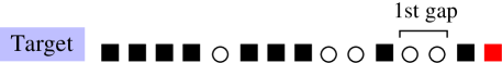
Figure 2: Illustration of different parking strategies for the same state of the parking lot: (a) meek, (b) prudent, and (c) optimistic. The red square denotes the newly parked car.

The meek driver wastes no time looking for a parking spot and just parks at the first available spot that is behind the most distant parked car. This strategy is risibly inefficient; many good parking spots are unfilled and most cars are parked far from the target. The prudent driver bets that there is at least one vacancy in the lot. If this bet is wrong, the prudent driver wastes the time to travel to $x=0$ and then backtracks to where it would have parked by employing the meek strategy. The optimistic driver bets that there is a spot close to the target and thus drives to the target and parks at the first vacancy encountered by backtracking (Fig. 2(c)). If a vacancy does not exist, the optimistic driver must also backtrack and park at the end of the line of parked cars.

3 Dynamics of the Number of Cars

A basic characterization of this parking process is the total number $N(t)$ of parked cars at time $t$. If we ignore the time spent in actually parking, the random variable $N(t)$ is independent of the parking strategy. The probability distribution $P_{N}(t)$ that there are $N$ parked cars at time $t$ satisfies the master equation

$$\frac{dP_{N}}{dt}=\lambda P_{N-1}+(N+1)P_{N+1}-(\lambda+N)P_{N}\,.$$ (1)

The first term on the right accounts for the gain in $P_{N}$ because a car parks in a lot with $N-1$ cars, the second term accounts for the gain in $P_{N}$ because a car leaves when the lot contains $N+1$ cars, and the last term accounts for the loss of $P_{N}$ because either a new car parks or a car leaves when the lot contains $N$ cars.

The solution to Eq. (1) can be obtained by the generating function method for an arbitrary initial condition (the derivation is given, e.g., in Ref. [22]). If the parking lot is initially empty, $P_{N}(0)=\delta_{N,0}$, the distribution of the number of parked cars is given by the Poisson distribution

$$P_{N}(t)=\frac{\big{[}\lambda(1-e^{-t})\big{]}^{N}}{N!}\,e^{-\lambda(1-e^{-t})}\,\,\xrightarrow[t\to\infty]{}\,\,\frac{\lambda^{N}}{N!}\,e^{-\lambda}\,.$$ (2)

From (2), the average number of parked cars is $\langle N(t)\rangle=\lambda(1-e^{-t})$, which approaches $\lambda$ in the long-time limit.

The actual number of parked cars fluctuates about the steady state value $\langle N\rangle=\lambda$, with the mean deviation from the average equal to $\sqrt{\langle N^{2}\rangle-\langle N\rangle^{2}}=\sqrt{\lambda}$. Huge fluctuations are also possible; for example, the parking lot empties with probability $P_{0}=e^{-\lambda}$. The average time $T$ between successive lot emptying events roughly scales as the reciprocal of this probability: $T\sim P_{0}^{-1}=e^{\lambda}$. Thus the emptying time is exponentially large in $\lambda$ for the interesting case of $\lambda\gg 1$; it is extremely unlikely that the lot is empty when arrival rate of new cars is large.

One can determine the emptying time by employing the backward Kolmogorov equation (see, e.g., [23, 14]) that relates the emptying time for a lot with $n$ cars to the emptying time for a parking lot with $n\pm 1$ cars. Let $t_{n}$ be the average time for the lot to empty starting from the state where $n$ cars are parked. This emptying time satisfies

$$t_{n}=p_{n}t_{n+1}+q_{n}t_{n-1}+\delta t_{n}\,.$$ (3)

The first term on the right-hand side accounts for the parking of a new car, an event that occurs with probability $p_{n}=\lambda/(\lambda+n)$. After this event, the average time for the parking lot to empty is $t_{n+1}$. The second term accounts a car leaving, which occurs with probability $q_{n}=n/(\lambda+n)$. Finally, $\delta t_{n}=1/(\lambda+n)$ is the average time for the number of parked cars to change from $n$ to $n\pm 1$.

Recurrences of the form (3) for general $p_{n},q_{n}$ and $\delta t_{n}$, are solvable (see, e.g., Chap. 12 of Ref. [14] and also [24]). Specializing the solution given there to the present case, the emptying time of the lot when $n$ cars are parked is

$$t_{n}=\frac{1}{\lambda}\sum_{j=0}^{n-1}\frac{j!}{\lambda^{j}}\sum_{i\geq j}\frac{\lambda^{i}}{i!}\,.$$ (4)

In the case where a single car is parked, this result simplifies to $t_{1}=(e^{\lambda}-1)/\lambda$. In the relevant case of $\lambda\gg 1$, all $t_{n}$ with $n\lesssim\lambda$ exhibit this same asymptotic behavior. For $\lambda\gg 1$, it is overwhelmingly likely that starting from a lot with a single parked car, the lot will quickly fill in a time of the order of 1 to its stationary value of $\lambda$ parked cars.

4 Meek Strategy

Models that resemble the meek strategy arise in various contexts, e.g., they have been used to mimic the evolution of genomic DNA [25, 26, 27] and they have been applied to modeling microtubule dynamics [22, 28, 29, 30]. The meek strategy is actually identical to the microtubule model discussed in  [22, 28]: a car that parks after the rightmost car corresponds to the addition of a GTP (guanosine triphosphate) monomer to the microtubule, and the departure of a car corresponds to the conversion for GTP to GDP (guanosine diphosphate). A catastrophe arises when the active end of a microtubule consists of only GDP monomers; these detach quickly, leading to a rapid decrease in the microtubule length. This latter event corresponds to a sudden drop in the span of parked cars when the rightmost car leaves and the next parked car is much closer to the target. The microtubule model is tractable, and the available analytical results [22, 28] provide a rather complete description of the car distribution that arises in the meek strategy. Below we outline some basic results and outline their derivations.

The meek strategy is ridiculously inefficient for $\lambda\gg 1$: the typical span, namely the distance from the target to the rightmost parked car, is huge, $L\propto e^{\lambda}$, while all cars are parked within a narrow populated region of length $\ell\simeq\lambda\ln\lambda$ near the right edge of the span (see Fig. 3). At any given moment the populated region moves nearly systematically to the right at speed $\lambda$ because of the continuous arrival of cars at this rate. Since the number of parked cars is roughly constant and they occupy a fixed-length region $\ell$, there typically is a huge empty space to the left of the populated region. This pattern is disrupted when a rare event occurs in which all cars in the populated region leave before a new car enters. When this happens, the parking process begins anew from an empty lot. The span therefore has a sawtooth time dependence (Fig. 4). When $\lambda\gg 1$, the emptying time is $T\simeq e^{\lambda}/\lambda$, and this gives an estimate $L\propto e^{\lambda}$: the emptying time is so large that we can only observe the growth of the span in simulations.

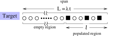
Figure 3: Schematic of the distribution of parked cars for the meek strategy in the large $\lambda$ limit. The span increases linearly in elapsed time from the last emptying event.

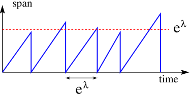
Figure 4: Schematic picture of the time dependence of the span in the meek parking strategy in the large $\lambda$ limit.

Let us estimate the behavior of the length $\ell$ of the populated region in the $\lambda\to\infty$ limit. Since cars leave the lot at rate 1, the probability that the car that is a distance $x$ from the rightmost car has not left the lot is $p(x)=e^{-\tau}=e^{-x/\lambda}$. To estimate the size of the populated region, we use the fact that the probability that there is a parked car located a distance $\ell$ or greater from the rightmost car is

$$\sum_{x\geq\ell}e^{-x/\lambda}=e^{-\ell/\lambda}/\big{(}1-e^{-1/\lambda}\big{)}\simeq\lambda\,e^{-\ell/\lambda}\,.$$ (5)

Setting this quantity to 1 gives a simple extreme statistics estimate for the size of the populated region (see, e.g., Refs. [31, 32]).

$$\ell=\lambda\ln\lambda\,.$$ (6)

Thus the length of the populated region is tiny compared to the span.

In the optimistic and prudent strategies the spatial distribution of parked cars quickly reaches and remains in a quasi-stationary state until the parking lot empties. Because newly arriving cars can park in the interior of the lot, spatial fluctuations in the span are of the order of $\sqrt{\lambda}$. Once again, a typical simulation with $\lambda\gg 1$ does not extend to the emptying time, so all that can be observed is the quasi steady-state behavior. We now study the spatial distribution of parked cars and related features for these two parking strategies.

5 Optimistic Strategy

The key feature of the optimistic strategy is that the dynamics of occupancy at any spot $i$ depends only on spots $1,2,\ldots,i$; all spots to right can be ignored. This property occurs in a number of one-dimensional systems that enjoy spatial causality, see e.g. [34, 35, 36, 37, 38], and it allows us to treat the optimistic strategy analytically.

Denote by $\sigma_{j}$ the occupation number of spot $j$:

$$\sigma_{j}=\begin{cases}1&\text{if $j$ is occupied}\,,\\ 0&\text{if $j$ is empty}\,.\end{cases}$$

The density $\rho_{1}=\langle\sigma_{1}\rangle$ at the first parking spot satisfies

$$\frac{d\rho_{1}}{dt}\equiv\dot{\rho}_{1}=\lambda(1-\rho_{1})-\rho_{1}\,,$$ (7)

which simply states that if the first spot is empty, it refills at rate $\lambda$, while if this spot is occupied, it empties with rate 1. The solution to this equation is

$$\rho_{1}=\frac{\lambda}{1+\lambda}\left[1-e^{-(1+\lambda)t}\right]\xrightarrow[t\to\infty]{}\,\,\frac{\lambda}{1+\lambda}$$ (8)

Following the same logic as in (7), the density $\rho_{k}$ satisfies the equation of motion

$$\dot{\rho}_{k}=\lambda\,\Big{\langle}(1-\sigma_{k})\prod_{j=1}^{k-1}\sigma_{j}\Big{\rangle}-\rho_{k}\,.$$ (9)

for any $k\geq 2$. These exact equations are not closed, viz., they involve the multisite averages $\langle\sigma_{1}\sigma_{2}\ldots\sigma_{k-1}\rangle$ and $\langle\sigma_{1}\sigma_{2}\ldots\sigma_{k-1}\sigma_{k}\rangle$. Writing evolution equations for these two averages involve other multisite averages. However, since the occupancy dynamics of the spots $1,2,\ldots,k$ does not depend on the spots $i>k$, the system of differential equations for $2^{k}-1$ multisite averages $\langle\sigma_{a}\ldots\sigma_{b}\rangle$, with $1\leq a<\ldots<b\leq k$, is closed. While the number of equations rapidly grows with $k$, they are linear, solvable, and can be treated recursively. We now illustrate this approach for $k=2$ and $k=3$.

5.1 $k=2$

When $k=2$, Eq. (9) becomes

$$\dot{\rho}_{2} =\lambda\rho_{1}-\rho_{2}-\lambda\langle\sigma_{1}\sigma_{2}\rangle=\lambda\rho_{1}-\rho_{2}-\lambda\rho_{12}$$ (10a)

$$\dot{\rho}_{12} =\lambda\langle(1-\sigma_{1})\sigma_{2}\rangle+\lambda\langle\sigma_{1}(1-\sigma_{2})\rangle-2\rho_{12}=\lambda(\rho_{1}+\rho_{2})-2(1+\lambda)\rho_{12}\,,$$ (10b)

where $\rho_{12}\equiv\langle\sigma_{1}\sigma_{2}\rangle$. The full time-dependent solutions to these equations are elementary but cumbersome. In the steady state

$$0=\lambda\rho_{1}-\rho_{2}-\lambda\rho_{12}$$ (11a)

$$0=\lambda(\rho_{1}+\rho_{2})-2(1+\lambda)\rho_{12}\,,$$ (11b)

from which

$$\rho_{12}=\frac{\lambda^{2}}{\lambda^{2}+2\lambda+2}\qquad\qquad\frac{\rho_{2}}{\rho_{12}}=\frac{\lambda+2}{\lambda+1}\,.$$ (12)

5.2 $k=3$

The equation for the density at site 3 is

$$\dot{\rho}_{3}=\lambda(\rho_{12}-\rho_{123})-\rho_{3}\,,$$ (13)

which involves the three-site average $\rho_{123}=\langle\sigma_{1}\sigma_{2}\sigma_{3}\rangle$. This average satisfies

$$\dot{\rho}_{123} =\lambda\langle(1-\sigma_{1})\sigma_{2}\sigma_{3}\rangle+\lambda\langle\sigma_{1}(1-\sigma_{2})\sigma_{3}\rangle+\lambda\langle\sigma_{1}\sigma_{2}(1-\sigma_{3})\rangle-3\rho_{123}$$

$$=\lambda(\rho_{12}+\rho_{23}+\rho_{13})-3(1+\lambda)\rho_{123}\,.$$ (14)

From (10b) we already know the nearest-neighbor two-site average $\rho_{12}=\langle\sigma_{1}\sigma_{2}\rangle$, and we also need the equations for $\rho_{13}=\langle\sigma_{1}\sigma_{3}\rangle$ and $\rho_{23}=\langle\sigma_{2}\sigma_{3}\rangle$:

$$\begin{split}&\dot{\rho}_{13}=\lambda\langle(1\!-\!\sigma_{1})\sigma_{3}\rangle+\lambda\langle\sigma_{1}\sigma_{2}(1\!-\!\sigma_{3})\rangle-2\rho_{13}=\lambda(\rho_{3}\!+\!\rho_{12}\!-\!\rho_{123})-(2\!+\!\lambda)\rho_{13}\\[5.69054pt] &\dot{\rho}_{23}=\lambda\langle\sigma_{1}(1\!-\!\sigma_{2})\sigma_{3}\rangle+\lambda\langle\sigma_{1}\sigma_{2}(1\!-\!\sigma_{3})\rangle-2\rho_{23}=\lambda(\rho_{13}\!+\!\rho_{12}\!-\!2\rho_{123})\!-\!2\rho_{23}\end{split}$$ (15)

Solving Eqs. (13)–(15) in the steady state gives

$$\rho_{123} =\frac{\lambda^{3}}{\lambda^{3}+3\lambda^{2}+6\lambda+6}\,,$$ (16a)

and in terms of this quantity, the remaining densities can be written as

$$\frac{\rho_{3}}{\rho_{123}} =\frac{\lambda^{2}+4\lambda+6}{\lambda^{2}+2\lambda+2}$$ (16b)

$$\frac{\rho_{23}}{\rho_{123}} =\frac{\lambda+3}{\lambda+2}$$ (16c)

$$\frac{\rho_{13}}{\rho_{123}} =\frac{(\lambda+1)(\lambda^{2}+4\lambda+6)}{(\lambda+2)(\lambda^{2}+2\lambda+2)}$$ (16d)

5.3 Decoupling approximation

While the exact results quickly become unwieldy, they greatly simplify in a decoupling approximation, in which we replace multi-site averages by the product of corresponding single-site averages (see, e,g, Ref. [33] for a general discussion of such decoupling approaches). For example, using $\rho_{12}=\rho_{1}\rho_{2}$ in (11a) gives

$$\rho_{2}^{\text{MF}}=\frac{\lambda^{2}}{\lambda^{2}+\lambda+1}\qquad\qquad\rho_{12}^{\text{MF}}=\frac{\lambda^{3}}{(\lambda^{2}+\lambda+1)(\lambda+1)}\,,$$ (17)

where the superscript MF denotes the mean-field densities that arise from the decoupling approximation. Similarly using $\rho_{12}=\rho_{1}\rho_{2}$ and $\rho_{123}=\rho_{1}\rho_{2}\rho_{3}$ in (5.2) gives

$$\rho_{3}^{\text{MF}}=\frac{\lambda^{4}}{\lambda^{4}+\lambda^{3}+2\lambda^{2}+2\lambda+1}\\$$ (18)

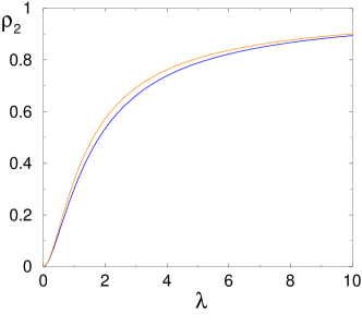
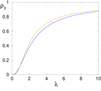
Figure 5: (a) The exact (blue) and decoupling approximation density (orange) at site 2 from (12) and (17), respectively. (b) Same for site 3. Here the exact density from (16a) lies below the decoupling approximation (19b) when $\lambda>0.900966$.

To gauge the accuracy of the decoupling approximation we compare the exact and approximate densities $\rho_{2}(\lambda)$ and $\rho_{3}(\lambda)$ in Fig. 5. The decoupling approximation is generally accurate and becomes more so accurate as $\lambda\to\infty$. To show this analytically, we define $\epsilon\equiv 1/(\lambda+1)$ as a small parameter, so that $\rho_{1}=1-\epsilon$. The expansion in $\epsilon$ yields

$$\rho_{2} =1-\epsilon-2\epsilon^{2}+2\epsilon^{3}+2\epsilon^{4}+\ldots$$

$$\rho_{2}^{\text{MF}} =1-\epsilon-\epsilon^{2}+\epsilon^{4}+\ldots$$

for the density and

$$\rho_{12} =1-2\epsilon+2\epsilon^{3}-2\epsilon^{5}+\ldots$$

$$\rho_{12}^{\text{MF}} =1-2\epsilon+\epsilon^{3}+\epsilon^{4}+\ldots$$

for the two-site correlation function. For $\rho_{2}$, the decoupling approximation expression is exact to second order in $\epsilon$, and $\rho_{12}$ is exact to third order. This pattern seems to hold for different sites; e.g., for the density at site 3 we expand (16a) and (18) and find that two leading orders of the expansion are again exact:

$$\begin{split}\rho_{3}&=1-\epsilon-4\epsilon^{2}-2\epsilon^{3}+\ldots\\ \rho_{3}^{\text{MF}}&=1-\epsilon-2\epsilon^{2}-2\epsilon^{3}+\ldots\end{split}$$

5.4 Large-$k$ behavior

Because the multisite correlation functions are cumbersome and the decoupling approximation is accurate, and even asymptotically exact in the most interesting $\lambda\to\infty$ limit, we now focus on the large-$k$ behavior using the decoupling approximation. In the steady state we obtain

$$\rho_{k+1}=\frac{\lambda\prod_{1\leq j\leq k}\rho_{j}}{1+\lambda\prod_{1\leq j\leq k}\rho_{j}}\,,$$ (19a)

which can be simplified to

$$\rho_{k+1}=\frac{\rho_{k}^{2}}{1-\rho_{k}+\rho_{k}^{2}}\,.$$ (19b)

Starting from $\rho_{1}={\lambda}/(1+\lambda)$ and iterating (19b), we find

$$n_{k+1}-n_{k}=\epsilon n_{k}^{2}\left[1-\frac{\epsilon^{2}n_{k}^{2}}{1-\epsilon n_{k}+\epsilon^{2}n_{k}^{2}}\right]\,,$$ (20)

where $\epsilon=1/(\lambda+1)$ and we have written the solution in the form $1-\rho_{k}=\epsilon n_{k}$.

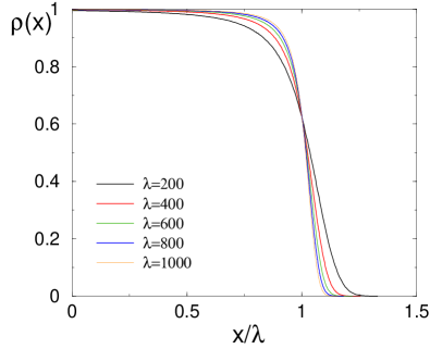
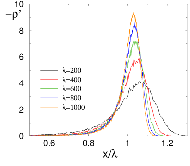
Figure 6: (a) The density of parked cars $\rho(x)$ as a function of distance $x$ from the target for the optimistic parking strategy for $\lambda$ between 200 and 1000. (b) The derivative $-d\rho/dx$. These curves have been smoothed over 1% of the data range.

Keeping only the leading term and replacing the difference by the derivative gives

$$\frac{dn_{k}}{dk}=\epsilon n_{k}^{2}\,,$$

whose solution, subject to the boundary condition $n_{1}=1$, yields

$$n_{k}=\frac{1}{1-\epsilon(k-1)}=\frac{\lambda+1}{\lambda+2-k}$$ (21a)

or equivalently

$$\rho_{k}=1-\frac{1}{\lambda+2-k}$$ (21b)

This solution applies in the “bulk” region where $\lambda-k\gg 1$. For small $k$, the density remains close to 1, but with a deviation that slows grows as $k$ increases.

Figure 6(a) shows simulation results for the steady-state density of parked cars for the optimistic strategy for representative value of $\lambda$. Our simulations start with an empty system and continue until roughly $10^{5}\lambda$ cars have parked. To give a more quantitative sense of the accuracy of (21b), Table 1 compares the prediction of this equation with simulation results.

Table 1: Comparison of $\rho_{k}$ from simulations (second column) and from Eq. (21b) (third column) for the case $\lambda=1000$.

$k$	$\rho_{k}$ (sim.)	$\rho_{k}$ (21b)
1	0.999004	0.999001
10	0.99898	0.99899
100	0.99877	0.99889
200	0.99845	0.99875
400	0.99724	0.99834

As $\lambda$ increases, the density of parked cars becomes more step-like and resembles the Fermi-Dirac distribution. To characterize the region near $x=\lambda$, Fig. 6(b) shows the derivative $-d\rho/dx$. The increasing steepness of the density step at $x=\lambda$ in Fig. 6(a) corresponds to the sharpening of the peak in Fig. 6(b). From the latter data, we also measure its width and find that this width shrinks roughly as $\lambda^{-1/2}$.

5.5 Vacancies

Let us now determine the location of the nearest open parking spot, or vacancy. The probability $V_{k}$ that the first vacancy is located at site $k$ is

$$V_{k}=\left\langle\prod_{j=1}^{k-1}\sigma_{j}\,(1-\sigma_{k})\!\right\rangle\,,$$ (22a)

which becomes, in the decoupling approximation,

$$V_{k}=\epsilon n_{k}\prod_{j=1}^{k-1}\rho_{j}\,.$$ (22b)

Taking the logarithm, replacing the sum by integration, and using (21b) we get

$$\sum_{j=1}^{k-1}\ln\rho_{j}\simeq\int_{1}^{k}dj\,\ln\!\left(1-\frac{1}{\lambda+2-k}\right)\simeq-\int_{1}^{k}\frac{dj}{\lambda+2-j}=\ln\frac{\lambda+2-k}{\lambda+1}\,.$$

Comparing with (21a), the product is

$$\prod_{j=1}^{k-1}\rho_{j}\simeq\frac{1}{n_{k}}\,.$$ (23)

Thus the location of the first vacancy is uniformly distributed in the range $[0,\lambda]$:

$$V_{k}=\begin{cases}\epsilon&k<\lambda\\ 0&k>\lambda\,,\end{cases}$$ (24)

from which the average position of the first vacancy is

$$v_{1}\equiv\langle k\rangle=\sum_{k=1}^{\lambda}kV_{k}=\frac{\lambda}{2}\,.$$ (25)

Our simulations are in excellent agreement with this simple result. The same approach can be applied to compute the joint probability $V_{k_{1},\ldots,k_{m}}$ to have $m$ vacancies at sites $k_{1}<k_{2}<\ldots<k_{m}<\lambda$. This probability is proportional to the product of the densities at the positions of all but the last vacancy, viz.,

$$V_{k_{1},\ldots,k_{m}}=\epsilon^{m}\prod_{a=1}^{m-1}n_{k_{a}}\,.$$ (26)

with $n_{k}$ given by (21a). In general, the average position of the $m^{\text{th}}$ vacancy is

$$v_{m}=(1-2^{-m})\lambda\,.$$ (27)

We anticipate that this result will hold as long as the $m^{\text{th}}$ vacancy is in the bulk of the density distribution.

6 Prudent Strategy and Comparison to Optimistic Strategy

The many-body nature of the parking process is more complicated for the case of the prudent strategy and our results for this case are simulational. Figure 7(a) shows the steady-state density of parked cars for the prudent strategy for representative value of $\lambda$. The salient feature of the prudent strategy is that there are lots of open parking spots very close to the target. This feature arises because a newly arriving car only penetrates to the first vacancy (or contiguous vacancy cluster) that it encounters. Thus parking spots that are close to the target are “screened” by more distant spots. Because it is unlikely that a new car penetrates to close parking spots and these spots open up with rate 1, the density of open spots near the target are likely to be high.

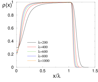
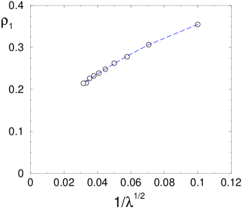
Figure 7: (a) The density of parked cars $\rho(x)$ as a function of distance $x$ from the target for the prudent parking strategy for $\lambda$ between 200 and 1000. (b) The average density of parked cars at the closest parking spot to the target, $\rho_{1}(\lambda)$, as a function of $1/\lambda^{1/2}$ for $\lambda$ in the range between 100 and 1000. The dashed line is a quadratic fit to these data that extrapolates to $\rho_{1}(\infty)\approx 0.11$.

To check this last hypotheses, we plot simulation data for the density of parked cars at site 1 as a function of $\lambda$ (Figure 7(b)). The data indicate that the average density of parked cars at the first spot, $\rho_{1}(\lambda)$, is a systematically decreasing function of $\lambda$ that extrapolates to a non-zero value for $\lambda\to\infty$. The quadratic fit shown in this figure extrapolates to $\rho_{1}(\infty)\approx 0.11$.

For both the optimistic and prudent strategies, the average span $L$ appears to have the asymptotic behavior $L\simeq\lambda+a\lambda^{1/2}$; more precisely

$$\lim_{\lambda\to\infty}\frac{L-\lambda}{\sqrt{\lambda}}=a$$ (28)

The amplitude $a>0$ is larger for the prudent strategy. Equation (28) implies that the number of vacancies grows as $a\sqrt{\lambda}$. Thus both the optimistic and prudent strategies are efficient in that there are generally very few open parking spots in the steady state. Figure 8(a) shows $L/\lambda$ plotted versus $1/\lambda^{1/2}$ for both the optimistic and prudent strategies. Both datasets show the same qualitative behavior in which $L/\lambda$ appears to extrapolate to 1 for $\lambda\to\infty$, with corrections that vanish as $1/\lambda^{1/2}$.

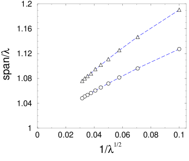
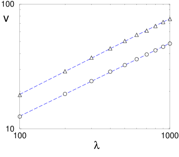
Figure 8: (a) The average span for the optimistic ($\circ$) and prudent ($\Delta$) strategies divided by $\lambda$ as a function of $1/\lambda^{1/2}$ for $\lambda$ in the range between 100 and 1000. The dashed curves are quadratic fits to these data. (b) The average number of open parking spots as a function of $\lambda$ for the optimistic ($\circ$) and prudent strategies ($\Delta$).

Figure 8(b) shows the dependence of the number of open parking spots on $\lambda$ for the both optimistic and prudent strategies. In both cases, the number of parking spots, $v$, appears to grow as $\lambda^{\nu}$, with $\nu\approx 0.58$. However, these data have a slight downward curvature and we expect that asymptotically $v\sim\lambda^{1/2}$.

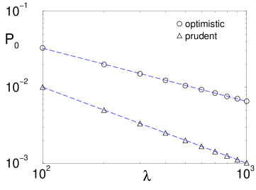
Figure 9: The Probability $P_{0}$ that the parking lot contains no open parking spaces as a function of $\lambda$.

A related measure of parking efficiency is the fraction of times that a driver has to backtrack to the end of the parked cars because there are no open spots available. This is the same as the probability $P_{0}$ that there are no open parking spots in the lot. As shown in Fig. 9, the fraction of parking attempts that requires the driver to backtrack to the end of the parking lot varies as $\lambda^{-\alpha}$ for both strategies, with $\alpha\approx 1$ for the prudent strategy and $\alpha\approx 0.7$ for the optimistic strategy.

7 Discussion

We introduced simple parking strategies in an idealized one-dimensional parking lot, viz. the semi-infinite line, with cars arriving one at a time at rate $\lambda$ and departing at rate 1. We assume that successive car arrivals are sufficiently separated in time that there is no competition between cars trying to park in the same spot. The number of parked cars is independent of the parking strategy. This number obeys a Poisson distribution, with the average number of parked cars equal to $\lambda$. However, the spatial distribution of parked cars strongly depends on the strategy that is employed.

In the meek strategy, each new car parks behind the most distant parked car. While this might be a reasonable approach when $\lambda$ is small, it quickly becomes ludicrous for large $\lambda$ because the position of the last car is typically a distance of the order of $e^{\lambda}$ from the target. However, if there are a few meek drivers while the majority follow the prudent or optimistic strategy, then the meek strategy is not bad because meek drivers will park a distance $\lambda$ from the target.

Much more practical are the optimistic and prudent strategies. In the optimistic strategy, a driver hopes that there is parking spot close to the target. Thus the driver goes all the way to the target, ignores all open spots, and finally parks at the first spot encountered upon backtracking. In the prudent strategy, the driver does not have the same degree of confidence but hopes that an open spots exists that is closer to the target than the most distant parked car; specifically, the prudent driver parks at the left end of the first gap.

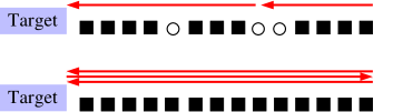
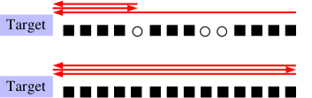
Figure 10: Schematic definition of the parking cost for the (a) prudent and (b) optimistic strategies for a parking lot with vacancies (top line) and for a full lot (bottom line).

Which strategy—optimistic or prudent—is better? To address this question quantitatively, one must introduce a cost of a parking event and compare the costs of the two strategies. A natural definition of cost is the distance from the parking spot to the target plus the time wasted in looking for a parking spot. To minimize the number of parameters, we assume that the speed of the car in the parking lot is the same as the walking speed. Thus an appropriate cost measure is the distance traveled by the car in the lot plus the distance that the driver walks from the parking spot to the target (Figure 10). With this definition of parking cost, the average cost scales linearly with $\lambda$, but with different prefactors for the optimistic and prudent strategies. On average, the prudent strategy is less costly. Thus even though the prudent strategy does not allow the driver to take advantage of the presence of many prime parking spots close to the target, the backtracking that must always occur in the optimistic strategy outweighs the benefit by typically parking closer to the target.

Needless to say, there are other ways to judge the efficacy of a parking strategy. Psychologically, a prudent driver may get upset by parking far from the target and then discovering that the closest parking spot is available. For the optimistic strategy this circumstance is impossible by construction, while for the prudent strategy it happens with probability close to $1-\rho_{1}$, i.e., approximately in 89% of all realizations. Another efficacy measure is the fraction of times a driver has to backtrack to the end of the parked cars because there are no open spots available. Fortunately for the driver, as $\lambda$ increases and the number of parked cars similarly increases, it becomes less likely that a parking attempt requires backtracking to the end of the parking lot.

With regard to parking, humans do not follow optimal strategies [39]. Instead, drivers tend to use simple heuristics, and the strategies outlined in this work are examples of such heuristics. Devising an optimal strategy is still an intriguing challenge. Adapting the methods from the optimal stopping research is not straightforward, e.g., in the parking problem studied in [16] the probability of a parking spot being occupied is independent of its location or of whether neighboring places are occupied. In our problem, the spatial distribution is emergent, and it also only statistically stationary.

References

- [1] D. Van Der Groot, Transportation Res. Part A: Policy and Practice 16, 109 (1982).
- [2] W. Young, R. G. Thompson, and M. A. P. Taylor, Transport Rev. 11, 63 (1991).
- [3] K. W. Axhausen and J. W. Polak, Transportation 18, 59 (1991).
- [4] R. G. Thompson and A. J. Richardson, Transportation Res. Part A: Policy and Practice, 32, 159 (1998).
- [5] R. Arnott and J. Rowse, J. Urban Economics 45, 97 (1999).
- [6] D. Teodorović and P. Luc̆ić, Eur. J. Oper. Res. 175, 1666 (2006).
- [7] A. Klappenecker, H. Lee, and J. L. Welch, Ad Hoc Networks 12, 243 (2014).
- [8] A. Renyi, Publ. Math. Inst. Hung. Acad. Sci. 3, 109 (1958).
- [9] J. V. Evans, Rev. Mod. Phys. 65, 1281 (1993).
- [10] P. L. Krapivsky and E. Ben-Naim, J. Chem. Phys. 100, 6778 (1994).
- [11] A. J. Kolan, E. R. Nowak, and A. V. Tkachenko, Phys. Rev. E 59, 3094 (1999).
- [12] J. Talbot, G. Tarjus, and P. Viot, Eur. Phys. J. E 5, 445 (2001).
- [13] M. Wackenhut and H. Herrmann, Phys. Rev. E 68, 041303 (2003).
- [14] P. L. Krapivsky, S. Redner, and E. Ben-Naim, A Kinetic View of Statistical Physics (Cambridge University Press, Cambridge, UK, 2010).
- [15] D. E. Knuth, The Art of Computer Programming, vol. 3: Sorting and Searching, ed. (Addison-Wesley, Reading, MA 1998).
- [16] J. MacQueen and R. G. Miller Jr., Oper. Res. 8, 362 (1960).
- [17] M. H. DeGroot, Optimal Statistical Decisions (McGraw-Hill, New York, 1970).
- [18] Y. S. Chow, H. Robbins and D. Siegmund Great Expectations: The Theory of Optimal Stopping (Houghton Mifflin Company, Boston, 1971).
- [19] B. A. Berezovsky and A. V. Gnedin, Problems of Best Choice (Akademia Nauk, Moscow, Russia, 1984).
- [20] T. S. Ferguson, Statistical Science 4, 282 (1989).
- [21] F. T. Bruss, Ann. Probab. 28, 1384 (2000).
- [22] T. Antal, P. L. Krapivsky, S. Redner, M. Mailman, and B. Chakraborty, Phys. Rev. E 74, 041907 (2007).
- [23] S. Redner, A Guide to First-Passage Processes (Cambridge University Press, Cambridge, UK, 2001).
- [24] S. Karlin and H. M. Taylor, A First Course in Stochastic Processes, ed. (Academic Press, San Diego, 1975).
- [25] W. Li, Phys. Rev. A 43, 5240 (1991).
- [26] P. W. Messer, M. Lässig, and P. F. Arndt, Phys. Rev. Lett. 94, 138103 (2005).
- [27] P. W. Messer, M. Lässig, and P. F. Arndt, J. Stat. Mech. P10004 (2005).
- [28] T. Antal, P. L. Krapivsky, and S. Redner, J. Stat. Mech. L05004 (2007).
- [29] P. Ranjith, D. Lacoste, K. Mallick, and J. F. Joanny, Biophys. J. 96, 2146 (2009).
- [30] C. Appert-Rolland, M. Ebbinghaus, and L. Santen, Phys. Repts. 593, 1 (2015).
- [31] J. Galambos, The Asymptotic Theory of Extreme Order Statistics (Wiley, New York, NY, 1987).
- [32] E. J. Gumbel, Statistics of Extremes (Dover Publications, Inc. Mineola, NY, 2004)
- [33] R. Balescu, Equilibrium and Non-Equilibrium Statistical Mechanics (Wiley, New York, 1975).
- [34] A. Mehta and J. M. Luck, J. Phys. A 36, L365 (2003).
- [35] L. S. Schulman, J. M. Luck, and A. Mehta, J. Stat. Phys. 146, 924 (2012).
- [36] A. Ayyer and K. Mallick, J. Phys. A 43, 045003 (2010).
- [37] A. Ayyer, J. Stat. Mech. P02034 (2011).
- [38] P. L. Krapivsky and J. M. Luck, arXiv:1902.04365.
- [39] T. Vanderbilt, Traffic: Why we drive the way we do (and what it says about us) (New York: Knopf, 2008).