Interpretable hypothesis tests

Victor Coscrato    Luís G. Esteves    Rafael Izbicki    Rafael B. Stern    Victor Coscrato
Federal University of São Carlos
   Luís Gustavo Esteves
University of São Paulo
   Rafael Izbicki
Federal University of São Carlos
   Rafael Bassi Stern
Federal University of São Carlos

Abstract

Abstract: Although hypothesis tests play a prominent role in Science, their interpretation can be challenging. Three issues are (i) the difficulty in making an assertive decision based on the output of an hypothesis test, (ii) the logical contradictions that occur in multiple hypothesis testing, and (iii) the possible lack of practical importance when rejecting a precise hypothesis. These issues can be addressed through the use of agnostic tests and pragmatic hypotheses.

Keywords: Hypothesis testing, agnostic tests, pragmatic hypothesesRunning title: Interpretable hypothesis tests

1 The elements of interpretable hypothesis tests

Although hypothesis tests play a prominent role in Science, its importance has been downplayed recently [Diggle and Chetwynd, 2011, Wasserman, 2013, Trafimow et al., 2018, Pike, 2019]. A major reason why hypothesis tests have been criticized is that they can be difficult to interpret and can even lead to misleading conclusions [Greenland et al., 2016, Kadane, 2016, Wasserstein et al., 2019]. At least three issues contribute to these challenges:

1. At least one of the outcomes of a standard hypothesis test is hard to interpret. While a standard hypothesis test can either reject or not reject the null hypothesis, the data can lead to at least three types of credal state: favor the null hypothesis, favor the alternate hypothesis, or remain undecided. Therefore, the test will assign to the same output at least two different credal states. For example, standard frequentist hypothesis tests usually do not control type II error probabilities. As a result, the non-rejection of the null hypothesis, $H_{0}$, can either be due to lack of evidence to reject $H_{0}$ or due to evidence in favor of $H_{0}$ [Fisher, 1959]. For instance, consider that $X\sim N(\theta,1)$ and $H_{0}:\theta\geq 0$. In a z-test, $H_{0}$ is not rejected no matter whether $X$ is close to $0$ or $X$ is very large. However, while in the former case there is little evidence in favor or against $H_{0}$, in the latter there is evidence in favor of $H_{0}$. Edwards et al. [1963] approaches this junction by stating that “if the null hypothesis is not rejected, it remains in a kind of limbo of suspended disbelief”. As a result, although in practice the non-rejection of $H_{0}$ is often taken as evidence in favor of $H_{0}$, this conclusion is not warranted by the test.

2. For standard Bayesian and classical tests, multiple hypothesis testing can lead to logically incoherent conclusions [Izbicki and Esteves, 2015, Fossaluza et al., 2017]. For example, for a given dataset, a test might reject $H_{0}:\theta\leq 0$ and not reject $H_{0}:\theta=0$, although the latter implies the former. Similarly, a test might reject both $H_{0}$ and $H_{0}^{*}$ but not reject $H_{0}\cup H_{0}^{*}$. These logical contradictions are hard to interpret and explain.

3. When a precise hypothesis is rejected, this outcome does not mean that the rejection is relevant from a practical perspective. For instance, consider that populations $1$ and $2$ are composed of, respectively, healthy and sick persons. Furthermore, for each person, one can observe a clinical variable, $X$, such as the patient’s average blood glucose level. Assume that, if $X_{i}$ is a person from population $i$, then $X_{i}\sim N(\theta_{i},1)$. Rejecting that the populations are the same, $H_{0}:\theta_{1}=\theta_{2}$, does not imply that $X$ can be used to determine whether a person is healthy or sick. For instance, when the sample size is large, one might reject $H_{0}$ although $|\theta_{1}-\theta_{2}|$ is not equal but close to $0$. In this case $X$ cannot effectively be used to determine whether a person is healthy or sick. This result can lead to counter-intuitive policies, such as considering an experiment to be inadequate from a statistical perspective because its sample size is too large [Faber and Fonseca, 2014]. Although solutions to this problem have been proposed, such as considering effect sizes [Cohen, 1992], they also increase the difficulty in interpreting hypothesis tests.

This paper shows that the above challenges in interpretation are avoided by making simple changes to the practice of hypothesis tests. These changes have two key components:

1. Agnostic hypothesis tests [Neyman, 1976, Berg, 2004], which parallel agnostic classifiers [Lei, 2014, Jeske and Smith, 2017, Jeske et al., 2017, Sadinle et al., 2017] and allow three possible results: reject $H_{0}$, accept $H_{0}$, or remain agnostic. The last option permits a test to control both the type I and type II errors [Coscrato et al., 2019], avoiding the “limbo of suspended disbelief” described in issue (i) that follows from the non-rejection of $H_{0}$ in standard tests. This occurs because the option of remaining agnostic allows the test to explicitly indicate when data does not provide substantial evidence either in favor or against $H_{0}$. Although agnostic tests introduce a type III error, which occurs whenever the test remains agnostic, this error is qualitatively different from the errors of type I and II. While it is unknown when the latter errors occur, the error of type III is known. Hence, the user of an agnostic test can control unknown errors and either acknowledge errors of type III or correct them by, for example, collecting more data. Besides these benefits, Esteves et al. [2016], Stern et al. [2017] show that, as opposed to standard tests, agnostic tests can guarantee logically coherent conclusions in multiple hypothesis testing, solving issue (ii).

2. Pragmatic hypothesis, which substitute precise hypotheses whenever the goal of the test is to determine variables with good predictive capabilities. For instance, let $X_{1}$ and $X_{2}$ be average blood glucose levels of healthy and sick persons and $X_{i}\sim N(\theta_{i},\sigma^{2})$. If one wishes to discover whether the blood glucose level is useful in determining whether an individual is healthy or sick, then the rejection of an hypothesis such as $Pg(H_{0}):|\theta_{1}-\theta_{2}|>k\sigma$ [Chow et al., 2016] is more informative than the rejection of $H_{0}:\theta_{1}\neq\theta_{2}$, which solves issue (iii). Similar ideas for augmenting the null hypothesis have previously been proposed in [Berger, 2013, DeGroot and Schervish, 2012].

The following sections define, illustrate and describe how to build agnostic tests and pragmatic hypotheses. This task requires additional notation. Specifically, the hypotheses that are considered are propositions about a parameter, $\theta\in\Theta\subseteq{\mathbb{R}}^{d}$. A null hypothesis is a proposition of the form $H_{0}:\theta\in{\Theta_{0}}$, where ${\Theta_{0}}\subseteq\Theta$ and the alternative hypothesis, $H_{1}$, is $H_{1}:\theta\in{\Theta_{0}^{c}}$. Whenever there is no ambiguity, ${\Theta_{0}}$ is used instead of $H_{0}$. In order to test $H_{0}$, data, ${\mathbf{X}}\in\mathcal{X}$, is used. Finally, the data follows a distribution given by ${\mathbb{P}}_{{\theta_{0}}}$ when $\theta={\theta_{0}}\in\Theta$.

2 Agnostic hypothesis tests

“The phrase ‘do not reject H’ is longish and cumbersome …(This action) should be distinguished from (the ones in) a ‘three-decision problem’ (in which the) actions are: (a) accept H, (b) reject H, and (c) remain in doubt.”

Neyman [1976]

A challenge in the interpretation of standard hypothesis tests is that they must always conclude one out of two possibilities. Although only two conclusions are available, data lead to at least three credal states: strongly disfavor $H_{0}$, strongly favor $H_{0}$ or not strongly favor or disfavor $H_{0}$. Standard tests usually assign the latter two states to the "non-rejection" of $H_{0}$. As a result, standard tests assign datasets which are qualitatively different to the same conclusion.

This challenge is addressed by agnostic tests, which can accept $H_{0}$ (0), reject $H_{0}$ (1) or remain undecided $\left(\frac{1}{2}\right)$. The set of possible outcomes of such a test is denoted by $\mathcal{D}=\left\{0,\frac{1}{2},1\right\}$.

Definition 2.1.

An agnostic test is a function, $\phi:\mathcal{X}\rightarrow\mathcal{D}$.

Definition 2.2.

An agnostic test, $\phi$, is a standard test if Im$[\phi]=\{0,1\}$.

An agnostic z-test is presented in Example 2.3.

Example 2.3.

Let $X\sim N(\theta,1)$. The usual $\alpha$-level z-test for $H_{0}:\theta_{0}\geq 0$ determines:

$$\begin{cases}\text{reject $H_{0}$}&\text{, if }X\leq\Phi^{-1}(\alpha)\\ \text{don't reject $H_{0}$}&\text{, if }X>\Phi^{-1}(\alpha)\end{cases}$$

For $\alpha=0.05$, $\Phi^{-1}(\alpha)$ is approximately $-1.64$. Therefore, no matter whether $x=-0.5$ or $x=10^{100}$, $H_{0}$ is not rejected. That is, no assertive decision about $H_{0}$ is obtained in either case although $x=10^{100}$ favors $H_{0}$ and $x=-0.5$ does not.

Alternatively, one can test $H_{0}$ with an agnostic test as follows:

$$\begin{cases}\text{reject $H_{0}$}&\text{, if }X<-\Phi^{-1}(0.5\alpha)\\ \text{accept $H_{0}$}&\text{, if }X>\Phi^{-1}(1-0.5\alpha)\\ \text{remain agnostic}&\text{, otherwise}\end{cases}$$ (1)

For $\alpha=0.05$, $\Phi^{-1}(1-0.5\alpha)$ is approximately $1.96$. Therefore, while $x=-0.5$ leads to an agnostic decision, $x=10^{100}$ leads to the assertive decision of accepting $H_{0}$. Contrary to the standard z-test, the agnostic test distinguishes these qualitatively different types of data.

An agnostic test can have $3$ types of errors. The type I and type II errors of agnostic tests are defined in the same way as those of standard tests. That is, a type I error occurs when the test rejects $H_{0}$ and $H_{0}$ is true. Similarly, a type II error occurs when the test accepts $H_{0}$ and $H_{0}$ is false. A type III error occurs whenever the test remains agnostic. That is, contrary to type I and type II errors, one knows when type III errors occur. Given this asymmetry, one might design either frequentist or Bayesian tests that control the errors of type I and II, as presented in Definition 2.4 and Definition 2.5.

Definition 2.4.

An agnostic test, $\phi$, has $(\alpha,\beta)$-level if the test’s probabilities of committing errors of type I and II are controlled by, respectively, $\alpha$ and $\beta$. That is,

$$\alpha_{\phi} :=\sup_{{\theta_{0}}\in H_{0}}{\mathbb{P}}_{{\theta_{0}}}(\phi=1)\leq\alpha$$

$$\beta_{\phi} :=\sup_{{\theta_{1}}\in H_{1}}{\mathbb{P}}_{{\theta_{1}}}(\phi=0)\leq\beta$$

Similarly, $\phi$, has size $(\alpha,\beta)$ if $\alpha_{\phi}=\alpha$ and $\beta_{\phi}=\beta$.

Definition 2.5.

An agnostic test, $\phi$, has false conclusion probability of $\gamma$ according to a prior distribution over $\theta$, $f_{\theta}:\Theta\rightarrow{\mathbb{R}}^{+}$, if

$$\gamma_{\phi} :=\int_{{\theta_{0}}\in H_{0}}{\mathbb{P}}_{{\theta_{0}}}(\phi=1)f_{\theta}({\theta_{0}})d{\theta_{0}}+\int_{{\theta_{1}}\in H_{1}}{\mathbb{P}}_{{\theta_{1}}}(\phi=0)f_{\theta}({\theta_{1}})d{\theta_{1}}=\gamma$$

There are several ways of controlling the errors above. For instance, [Esteves et al., 2016, Coscrato et al., 2019] discuss approaches based on statistical decision theory. The following subsection presents an agnostic test that controls the errors above while preserving other properties, such as logical consistency.

2.1 Region-based agnostic tests

Agnostic tests can be constructed through region estimators. A region estimator is a function that assigns a subset of the parameter space to each possible dataset. Generally, a region estimator can be interpreted as a set of plausible values for $\theta$. For instance, when $\Theta={\mathbb{R}}$, confidence and credible intervals are region estimators.

Definition 2.6.

A region estimator, $R$, is a function from $\mathcal{X}$ such that $R({\mathbf{x}})\subseteq\Theta$.

It is possible to completely specify an agnostic test by means of a region estimator. Based on the idea that the region estimator indicates the plausible values for $\theta$, there are three cases to consider. If all plausible values lie in $H_{0}$, then there is strong evidence in favor of $H_{0}$ and $H_{0}$ is accepted. Also, if all plausible values lie outside of $H_{0}$, then there is strong evidence against $H_{0}$ and $H_{0}$ is rejected. Finally, if there are plausible values both in and outside of $H_{0}$, then $H_{0}$ remains undecided. Definition 2.7 formalizes this description.

Definition 2.7.

The agnostic test based on $R$ for testing $H_{0}$, $\phi$, illustrated in Figure 1, is

$$\phi({\mathbf{x}}) =\begin{cases}0&\text{, if }R({\mathbf{x}})\subseteq H_{0}\\ 1&\text{, if }R({\mathbf{x}})\subseteq H_{0}^{c}\\ \frac{1}{2}&\text{, otherwise.}\\ \end{cases}$$

Figure 1: $\phi({\mathbf{x}})$ is an agnostic test based on the region estimator, $R({\mathbf{x}})$, for testing $H_{0}$.

If an agnostic tests is based on a region estimator that is a (frequentist) confidence set, then the size of the test is controlled, as described in Theorem 2.8.

Theorem 2.8 (Coscrato et al. [2019]).

If $R({\mathbf{x}})$ is a region estimator for $\theta$ with confidence $1-\alpha$ and $\phi$ is an agnostic test for $H_{0}$ based on $R$ (Definition 2.7), then $\phi$ is a $(\alpha,\alpha)$-level test. Also, for every prior distribution over $\theta$, $f_{\theta}$, $\gamma_{\phi}\leq\alpha$ according to $f_{\theta}$.

Similarly, if an agnostic test is based on a (Bayesian) credible set instead of a confidence set, then it controls the false conclusion probability, as described in Theorem 2.9.

Theorem 2.9.

If $R({\mathbf{x}})$ is a region estimator for $\theta$ with credibility $1-\gamma$ according to $f_{\theta}$ and $\phi$ is an agnostic test for $H_{0}$ based on $R$ (Definition 2.7), then $\gamma_{\phi}\leq\gamma$ according to $f_{\theta}$.

Example 2.3 below shows how Theorems 2.8 and 2.9 can construct agnostic z-tests.

Example 2.10 (Continuation of Example 2.3).

The agnostic test in Example 2.3 can be obtained from Theorem 2.8 by using the usual ($1-\alpha$)-level confidence interval given by $CI=[X-\Phi^{-1}(0.5\alpha),X-\Phi^{-1}(1-0.5\alpha)]$. The obtained test has $(\alpha,\alpha)$-level.

One can also test $H_{0}$ by applying Theorem 2.9. If $\theta\sim N(0,1)$, then a typical $1-\gamma$ credible interval for $\theta$ is $CI=\left[0.5X-\frac{\Phi^{-1}(0.5\gamma)}{\sqrt{2}},0.5X-\frac{\Phi^{-1}(1-0.5\gamma)}{\sqrt{2}}\right]$. The test based on this interval controls the false conclusion probability by $\gamma$ and behaves similarly to the test in eq. 1.

An example of a test based on a credible sets is the Generalized Full Bayesian Significance Test (GFBST) [Stern et al., 2017], which is obtained when the credibility set is a highest posterior density set. Theorem 2.9 shows that the GFBST controls the false conclusion probability.

Another useful property of tests based on region estimators, such as the ones obtained from Theorems 2.8 and 2.9, is that they are the only logically coherent tests [Esteves et al., 2016]. That is, if the same region estimator is used for simultaneously testing several hypothesis, then there will be no logical contradiction between the conclusions of the tests. For instance, a standard t-test can reject $\theta\leq 0$ and not reject $\theta=0$. Since $\theta\leq 0$ is implied by $\theta=0$, such a result is a logical contradiction. If an agnostic test based on a region estimator rejects $\theta\leq 0$, then it also rejects $\theta=0$.

It follows from the logical coherence of agnostic tests based on region estimators that they are consistent with propositional logic [Stern et al., 2017][Lemma 6.1]. For example, consider a class of agnostic tests, $\phi$, based on the same region estimator, two hypotheses, $H_{1}$ and $H_{2}$, and the logical proposition $H^{*}=P(H_{1},H_{2})=(H_{1}\cap H_{2})^{c}$. Since $\phi$ is consistent with propositional logic, the outcome of testing $H^{*}$ with $\phi$ can be determined by the outcome of testing $H_{1}$ and $H_{2}$ with $\phi$. For example, if $\phi$ rejects either $H_{1}$ or $H_{2}$, then it accepts $H^{*}$, if $\phi$ accepts $H_{1}$ and $H_{2}$, then it rejects $H^{*}$, and otherwise it remains agnostic about $H^{*}$. The consistency with propositional logic not only makes the test easier to interpret but also makes simultaneous hypothesis testing easier to implement. The latter occurs since calculating the truth-value of a proposition is generally less expensive computationally than a direct calculation of the test.

Despite the advantages of region-based agnostic tests over standard test, the former usually do not accept precise hypotheses. For instance, if $H_{0}:\theta=0$, then whenever a confidence interval contains more than a single point, it follows from Definition 2.7 that $H_{0}$ is not accepted. The following section argues that this result is justifiable. From a practical perspective, whenever one wishes to be able to accept the null hypothesis, this hypothesis can be well represented by a pragmatic hypothesis.

3 Pragmatic hypotheses

“The null hypothesis is really a hazily defined small region rather than a point.”

Edwards et al. [1963]

When the null hypothesis is stated as an equality, it is often reasonable to enlarge it to a set of values which are close to satisfying the equality from a practical perspective. Such an enlarged hypothesis is called a pragmatic hypothesis. Although in some situations the pragmatic hypothesis might be derived from expert knowledge, this solution might not always be available. This section presents a method for deriving pragmatic hypotheses which closely resembles the ones in Esteves et al. [2018].

We assume that the researcher is interested in predicting a future experiment, ${\mathbf{Z}}\in\mathcal{Z}$, which is distributed according to a density, $f_{{\mathbf{Z}}}({\mathbf{z}}|\theta)$. This future experiment can be different from ${\mathbf{X}}$, which is used to test the hypothesis. Specifically, the hypothesis is tested in the present using ${\mathbf{X}}$ so that accurate predictions about ${\mathbf{Z}}$ can be made in the future.

For a given future experiment ${\mathbf{Z}}$, one can determine which values of $\theta$ make ${\mathbf{Z}}$ behave similarly. A predictive dissimilarity function, $d_{{\mathbf{Z}}}:\Theta^{2}\rightarrow{\mathbb{R}}^{+}$ is a function $d_{{\mathbf{Z}}}({\theta_{0}},{\theta^{*}})$ that measures how much ${\mathbf{Z}}$ behaves differently under ${\theta_{0}}$ and under ${\theta^{*}}$. We focus on the classification dissimilarity:

$$d_{{\mathbf{Z}}}({\theta_{0}},{\theta^{*}}) =0.5\left({\mathbb{P}}_{{\theta_{0}}}\left(\frac{f({\mathbf{Z}}|{\theta_{0}})}{f({\mathbf{Z}}|{\theta^{*}})}>1\right)+{\mathbb{P}}_{{\theta^{*}}}\left(\frac{f({\mathbf{Z}}|{\theta^{*}})}{f({\mathbf{Z}}|{\theta_{0}})}>1\right)\right)$$ (2)

The classification dissimilarity can be interpreted using the Neyman-Pearson lemma [Neyman and Pearson, 1933] as follows. Consider that ${\mathbf{Z}}$ was generated with equal probability either from ${\theta_{0}}$ or from ${\theta^{*}}$. After observing ${\mathbf{Z}}$ in such a situation, the classification dissimilarity is the highest achievable probability of correctly identifying which $\theta$ generated ${\mathbf{Z}}$.

Once a predictive dissimilarity function is chosen, the pragmatic hypothesis associated to $H_{0}$, $Pg(H_{0})$, is defined as the set of parameter values whose dissimilarity to $H_{0}$ is at most $1-\epsilon$:

$$Pg(H_{0}) =\bigcup_{{\theta_{0}}\in H_{0}}\left\{{\theta^{*}}\in\Theta:d_{{\mathbf{Z}}}({\theta_{0}},{\theta^{*}})<1-\epsilon\right\}.$$

If ${\theta^{*}}\notin Pg(H_{0})$, then ${\mathbf{Z}}$ can be used to discriminate between ${\theta^{*}}$ and any given point in $H_{0}$ with an accuracy of at least $1-\epsilon$.

This construction can be illustrated with a test of equality between populations. In this case, if a parameter value lies outside of the pragmatic hypothesis, then there exists a classifier based on ${\mathbf{Z}}$ with accuracy of at least $1-\epsilon$ for determining which population generated ${\mathbf{Z}}$ (Theorem A.1). This procedure is applied to real data in Example 3.1.

Example 3.1.

The Cambridge Cognition Examination (CAMCOG) [Roth et al., 1986] is a questionnaire that is used to measure the extent of dementia and assess the level of cognitive impairment. We use the data from Cecato et al. [2016] to check whether CAMCOG is able to distinguish three groups of patients: (i) control (CG), (ii) mild cognitive impairment (MCI), and (iii) Alzheimer’s disease (AD). We assume that, if $Y_{i,j}$ is the score of the $j$-th patient in group $i$, then $Y_{i,j}=\mu_{i}+\epsilon_{i,j}$, where $\mu_{i}$ are the population averages in each group and $\epsilon_{i,j}$ are independent variables such that $\epsilon_{i,j}\sim N(0,\sigma^{2})$.

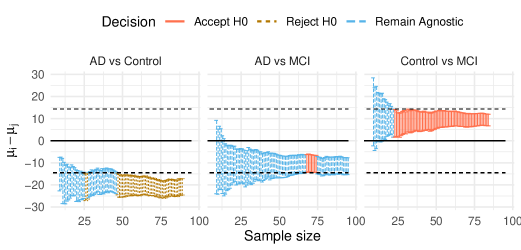
Figure 2: Confidence intervals for the average difference between groups, $\mu_{i}-\mu_{j}$ as a function of the sample size. The solid line indicates the precise hypothesis considered in each figure, $H_{0}:\mu_{i}=\mu_{j}$. The dashed horizontal lines delimit the pragmatic null hypotheses that are induced by each precise hypothesis.

Figure 2 illustrates how the sample size affects region-based agnostic tests (Definition 2.7) for testing the pragmatic hypotheses induced by $H_{0}:\mu_{i}-\mu_{j}=0$. In each of the plots, the solid line indicates the precise hypothesis of interest, that is, the CAMCOG scores are equally distributed among the compared groups. The values of $\mu_{i}-\mu_{j}$ between the dashed lines compose the associated pragmatic hypothesis, $Pg(H_{0})$. When the pragmatic hypothesis does not hold, there exists a classifier based on the CAMCOG score which highly discriminates the groups under comparison. For small sample sizes, the test remains agnostic about all of the three hypotheses. As the sample size increases, the pragmatic hypothesis associated to AD vs Control is rejected, the one for AD vs MCI is undecided and the one for Control vs MCI is accepted. That is, although it is unclear whether a classifier based on the CAMCOG score can highly discriminate between patients with AD and MCI, it can highly discriminate between AD and Control and cannot highly discriminate between Control and MCI. Since AD is an aggravation of MCI, these conclusions are compatible with qualitative knowledge.

In situations with several parameters, it can be expensive to compute $Pg(H_{0})$ exactly. In these cases, it is possible to calculate an approximation of $Pg(H_{0})$. For example, let $\theta(i)$ denote the i-th coordinate of $\theta$ and consider that $H_{0}:\theta(1)={\theta_{0}}$. In this case, an approximate pragmatic hypothesis, $Pg^{*}(H_{0})$, can be obtained by considering that the remaining parameter coordinates are equal to a given estimate. Specifically,

1. Estimate $\theta(2),\ldots,\theta(d)$ based on ${\mathbf{X}}$ with $\hat{\theta}(2),\ldots,\hat{\theta}(d)$.

2. Define $g:{\mathbb{R}}\rightarrow{\mathbb{R}}^{d}$ such that $g(t)=\left(t,\hat{\theta}(2),\ldots,\hat{\theta}(d)\right)$.

3. Let $Pg^{*}(H_{0})=\left\{{\theta^{*}}\in{\mathbb{R}}:d_{{\mathbf{Z}}}(g({\theta_{0}}),g({\theta^{*}}))\leq\epsilon\right\}\times{\mathbb{R}}^{d-1}$.

Algorithm 1 in Section A.2 shows how such a procedure can be applied to a generic model using Monte Carlo integration. An implementation of this procedure in R is available at https://github.com/vcoscrato/pragmatic. Example 3.2 illustrates this procedure in the context of linear regression.

Example 3.2.

An object dropped from a vertical distance $d$ from the ground takes $T=\sqrt{\frac{2d}{g}}$ units of time to reach the floor, where $g$ is Earth’s gravitational acceleration. Diggle and Chetwynd [2011, Chapter 2] describes a lab experiment for estimating $g$: a student drops an object from several heights and measures how long it takes to reach the ground by using a chronometer. Since the student has a reaction for activating and deactivating the chronometer, the data may be modeled as

$$T =\beta_{0}+\beta_{1}x+\epsilon, \text{where }x=\sqrt{d},\beta_{1}=\sqrt{2g^{-1}}\text{ and }\epsilon\sim N(0,1)$$

One might be interested in testing $H_{0}:g=9.8$. Besides $g$, the parameter space also includes the average reaction time of the students, $\beta_{0}$ and the imprecision in their measurements, $\sigma^{2}$. Although obtaining $Pg(H_{0})$ is not intractable in this case, it would involve a search in a three-dimensional space. This procedure is simplified when calculating $Pg^{*}(H_{0})$, in which $\beta_{0}$ and $\sigma^{2}$ are considered to be equal to their estimates that are obtained from the observed sample, ${\mathbf{X}}$. As a result, determining $Pg^{*}(H_{0})$ involves a search over a one-dimensional space only.

Figure 3 illustrates how the sample size affects region-based agnostic tests for $Pg^{*}(H_{0})$. In the left and right plots, the precise hypotheses are that, respectively, $H_{0}:g=9.5$ and $H_{0}:g=9.8$. In each plot, the values of $g$ delimited between the horizontal dashed lines constitute the pragmatic null hypotheses, $Pg^{*}(H_{0})$. These pragmatic hypotheses are composed by values of $g$ which would induce predictions for future experiments in a similar way as each precise hypothesis. These pragmatic hypotheses are tested with a region-based agnostic test. For small sample sizes, the test remains undecided about both pragmatic hypotheses. As the sample size increases, the test rejects that $g$ is close to $9.5$ and accepts that $g$ is close to $9.8$. The latter conclusion might seem incorrect, since $g\approx 9.807$. However, given the high imprecision in the experiment performed by the students, future experiments would behave similarly no matter whether $g=9.807\ldots$ or $g=9.8$.

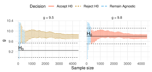
Figure 3: Confidence intervals for the gravitational constant $g$ as a function of the sample size. The solid line indicates the precise hypothesis considered in each figure. The dashed horizontal lines delimit the pragmatic null hypotheses that are induced by each precise hypothesis.

4 Conclusions and future research

Challenges in the interpretation of standard hypothesis tests can be addressed through changes in statistical practice. Agnostic hypothesis tests lead to test outputs that are easier to interpret and also avoid logical contradictions in multiple hypothesis testing. Also, the use of pragmatic hypotheses render that the rejection of the null hypothesis is of practical importance. Examples 3.1 and 3.2 illustrate how these improvements admit a simple implementation in standard models.

This paper also provides a general method for obtaining approximate pragmatic hypotheses in parametric statistical models. Future research might involve obtaining pragmatic hypothesis in nonparametric models and a decision-theoretic approach to agnostic tests.

Acknowledgments

This study was also financed in part by the Coordenação de Aperfeiçoamento de Pessoal de Nível Superior - Brasil (CAPES) - Finance Code 001. Rafael Izbicki is grateful for the financial support of FAPESP (2017/03363-8) and CNPq (306943/2017-4).

Appendix A Appendix

A.1 Proofs

Proof of Theorem 2.9.

$$\gamma_{\phi} =\int_{{\theta_{0}}\in H_{0}}{\mathbb{P}}_{{\theta_{0}}}(\phi({\mathbf{X}})=1)f_{\theta}({\theta_{0}})d{\theta_{0}}+\int_{{\theta_{1}}\in H_{1}}{\mathbb{P}}_{{\theta_{1}}}(\phi({\mathbf{X}})=0)f_{\theta}({\theta_{1}})d{\theta_{1}}$$

$$=\int_{{\theta_{0}}\in H_{0}}{\mathbb{P}}_{{\theta_{0}}}(R({\mathbf{X}})\subset H_{0}^{c})f_{\theta}({\theta_{0}})d{\theta_{0}}+\int_{{\theta_{1}}\in H_{1}}{\mathbb{P}}_{{\theta_{1}}}(R({\mathbf{X}})\subset H_{0})f_{\theta}({\theta_{1}})d{\theta_{1}}$$

$$\leq\int_{{\theta_{0}}\in H_{0}}{\mathbb{P}}_{{\theta_{0}}}({\theta_{0}}\notin R({\mathbf{X}}))f_{\theta}({\theta_{0}})d{\theta_{0}}+\int_{{\theta_{1}}\in H_{1}}{\mathbb{P}}_{{\theta_{1}}}({\theta_{1}}\notin R({\mathbf{X}}))f_{\theta}({\theta_{1}})d{\theta_{1}}$$

$$\leq\int_{{\theta^{*}}\in\Theta}{\mathbb{P}}_{{\theta^{*}}}({\theta^{*}}\notin R({\mathbf{X}}))f_{\theta}({\theta^{*}})d{\theta^{*}}=\gamma R({\mathbf{X}}) (1-\gamma)$$ has credibility

∎

Theorem A.1.

Let ${\mathbf{Z}}=(Z_{0},Z_{1})$ and $\theta=(\theta_{0},\theta_{1})$ be such that $f(z_{0},z_{1}|\theta_{0},\theta_{1})=f(z_{0}|\theta_{0})f(z_{1}|\theta_{1})$. Also, $H_{0}:\theta_{0}=\theta_{1}$, $Y\sim\text{Bernoulli}(0.5)$ and $Z^{*}=Z_{Y}$. If $\theta^{*}\notin Pg(H_{0})$ and ${\mathbf{Z}}\sim f_{\theta^{*}}$, then it is possible to build a classifier with accuracy of at least $1-\epsilon$ for $Y$ using $Z^{*}$.

Proof.

If ${\theta^{*}}\notin Pg(H_{0})$, then for every $\bar{\theta}\in H_{0}$, $CD(\bar{\theta},{\theta^{*}})\geq 1-\epsilon$. In particular, by choosing $\bar{\theta}=({\theta^{*}_{1}},{\theta^{*}_{1}})$, obtain that $CD(({\theta^{*}_{1}},{\theta^{*}_{1}}),{\theta^{*}})\geq 1-\epsilon$. Therefore,

$$1-\epsilon \leq CD(({\theta^{*}_{1}},{\theta^{*}_{1}}),{\theta^{*}})$$

$$=0.5\left({\mathbb{P}}_{({\theta^{*}_{1}},{\theta^{*}_{1}})}\left(\frac{f_{({\theta^{*}_{1}},{\theta^{*}_{1}})}({\mathbf{Z}})}{f_{{\theta^{*}}}({\mathbf{Z}})}>1\right)+{\mathbb{P}}_{{\theta^{*}}}\left(\frac{f_{{\theta^{*}}}({\mathbf{Z}})}{f_{({\theta^{*}_{1}},{\theta^{*}_{1}})}({\mathbf{Z}})}>1\right)\right)$$

$$=0.5\left({\mathbb{P}}_{({\theta^{*}_{1}},{\theta^{*}_{1}})}\left(\frac{f_{{\theta^{*}_{1}}}(Z_{1})f_{{\theta^{*}_{1}}}(Z_{2})}{f_{{\theta^{*}_{1}}}(Z_{1})f_{{\theta^{*}_{2}}}(Z_{2})}>1\right)+{\mathbb{P}}_{{\theta^{*}}}\left(\frac{f_{{\theta^{*}_{1}}}(Z_{1})f_{{\theta^{*}_{2}}}(Z_{2})}{f_{{\theta^{*}_{1}}}(Z_{1})f_{{\theta^{*}_{1}}}(Z_{2})}>1\right)\right)$$

$$=0.5\left({\mathbb{P}}_{{\theta^{*}_{1}}}\left(\frac{f_{{\theta^{*}_{1}}}(Z_{2})}{f_{{\theta^{*}_{2}}}(Z_{2})}>1\right)+{\mathbb{P}}_{{\theta^{*}_{2}}}\left(\frac{f_{{\theta^{*}_{2}}}(Z_{2})}{f_{{\theta^{*}_{1}}}(Z_{2})}>1\right)\right)$$ (3)

The proof follows since section A.1 is the accuracy of the Bayes classifier [Wasserman, 2013] for $Y$ using $Z^{*}$. ∎

A.2 Approximate pragmatic hypotheses

Algorithm 1 Approximate pragmatic hypothesis computation for $H_{0}:\theta(1)=\theta_{0}$

Input: Null hypothesis parameter value $\theta_{0}$; estimates of $\theta(2),\ldots,\theta(d)$ based on the observed data, $\widehat{\theta}(2),\ldots,\widehat{\theta}(d)$; dissimilarity threshold $0.5\leq\epsilon\leq 1$; function log_f(${\mathbf{z}};\theta$) that computes the log-likelihood function of the new experiment; function generate_samples($\theta$) that generates new samples ${\mathbf{Z}}$ from the distribution $f({\mathbf{z}}|\theta)$; number of Monte Carlo simulations $B$ Output: Approximate pragmatic hypothesis $Pg^{*}(H_{0})$ 1:Let $\bar{\theta}_{0}\leftarrow(\theta_{0},\widehat{\theta}(2),\ldots,\widehat{\theta}(d))$ 2:for $i=1,\ldots,B$ do 3:     ${\mathbf{z}}^{0}_{i}=$ generate_samples($\bar{\theta}_{0}$) 4:end for 5:Let $Pg^{*}(H_{0})\leftarrow\emptyset$ 6:for $\theta^{*}\in\mathbb{R}$ do 7:     Let $\bar{\theta}^{*}\leftarrow(\theta^{*},\widehat{\theta}(2),\ldots,\widehat{\theta}(d))$ 8:     for $i=1,\ldots,B$ do 9:         ${\mathbf{z}}^{*}_{i}=$ generate_samples($\bar{\theta}^{*}$) 10:     end for 11:     Let $\text{correct}_{\theta_{0}}\leftarrow\text{mean}\left({\mathbb{I}}\left(\text{log\_f}({\mathbf{z}}^{0}_{i};\bar{\theta}_{0})>\text{log\_f}({\mathbf{z}}^{0}_{i};\bar{\theta}^{*})\right)_{i=1}^{B}\right)$ 12:     Let $\text{correct}_{\theta^{*}}\leftarrow\text{mean}\left({\mathbb{I}}\left(\text{log\_f}({\mathbf{z}}^{*}_{i};\bar{\theta}^{*})>\text{log\_f}({\mathbf{z}}^{*}_{i};\bar{\theta}_{0})\right)_{i=1}^{B}\right)$ 13:     Let $\text{dist}=2^{-1}\left(\text{correct}_{\theta_{0}}+\text{correct}_{\theta^{*}}\right)$ 14:     if dist$<\epsilon$ then 15:         $Pg^{*}(H_{0})\leftarrow Pg^{*}(H_{0})\cup\{\theta^{*}\}$ 16:     end if 17:end for 18:return $Pg^{*}(H_{0})$

References

- Diggle and Chetwynd [2011] P. J. Diggle and A. G. Chetwynd. Statistics and scientific method: an introduction for students and researchers. Oxford University Press, 2011.
- Wasserman [2013] L. Wasserman. All of statistics: a concise course in statistical inference. Springer Science & Business Media, 2013.
- Trafimow et al. [2018] David Trafimow, Valentin Amrhein, Corson N Areshenkoff, Carlos J Barrera-Causil, Eric J Beh, Yusuf K Bilgiç, Roser Bono, Michael T Bradley, William M Briggs, Héctor A Cepeda-Freyre, et al. Manipulating the alpha level cannot cure significance testing. Frontiers in Psychology, 9, 2018.
- Pike [2019] Harriet Pike. Statistical significance should be abandoned, say scientists. BMJ, 364, 2019. ISSN 0959-8138. 10.1136/bmj.l1374. URL https://www.bmj.com/content/364/bmj.l1374.
- Greenland et al. [2016] S. Greenland, S. J. Senn, K. J. Rothman, J. B. Carlin, C. Poole, S. N. Goodman, and D. G. Altman. Statistical tests, p values, confidence intervals, and power: a guide to misinterpretations. European journal of epidemiology, 31(4):337–350, 2016.
- Kadane [2016] J. B. Kadane. Beyond hypothesis testing. Entropy, 18(5):199, 2016.
- Wasserstein et al. [2019] Ronald L. Wasserstein, Allen L. Schirm, and Nicole A. Lazar. Moving to a world beyond . The American Statistician, 73(sup1):1–19, 2019. 10.1080/00031305.2019.1583913. URL https://doi.org/10.1080/00031305.2019.1583913.
- Fisher [1959] Sir Ronald A Fisher. Mathematical probability in the natural sciences. Technometrics, 1(1):21–29, 1959.
- Edwards et al. [1963] Ward Edwards, Harold Lindman, and Leonard J Savage. Bayesian statistical inference for psychological research. Psychological review, 70(3):193, 1963.
- Izbicki and Esteves [2015] Rafael Izbicki and Luís Gustavo Esteves. Logical consistency in simultaneous statistical test procedures. Logic Journal of the IGPL, 23(5):732–758, 2015.
- Fossaluza et al. [2017] V. Fossaluza, R. Izbicki, G. M. da Silva, and L. G. Esteves. Coherent hypothesis testing. The American Statistician, 71(3):242–248, 2017.
- Faber and Fonseca [2014] Jorge Faber and Lilian Martins Fonseca. How sample size influences research outcomes. Dental press journal of orthodontics, 19(4):27–29, 2014.
- Cohen [1992] Jacob Cohen. A power primer. Psychological bulletin, 112(1):155, 1992.
- Neyman [1976] Jerzy Neyman. Tests of statistical hypotheses and their use in studies of natural phenomena. Communications in statistics-theory and methods, 5(8):737–751, 1976.
- Berg [2004] N. Berg. No-decision classification: an alternative to testing for statistical significance. The Journal of Socio-Economics, 33(5):631–650, 2004.
- Lei [2014] J. Lei. Classification with confidence. Biometrika, 101(4):755–769, 2014.
- Jeske and Smith [2017] D. R. Jeske and S. Smith. Maximizing the usefulness of statistical classifiers for two populations with illustrative applications. Statistical methods in medical research, 2017.
- Jeske et al. [2017] D. R. Jeske, J. A. Linehan, T. G. Wilson, M. H. Kawachi, K. Wittig, K. Lamparska, C. Amparo, R. Mejia, F. Lai, D. Georganopoulou, and S. S. Steven. Two-stage classifiers that minimize pca3 and the psa proteolytic activity testing in the prediction of prostate cancer recurrence after radical prostatectomy. The Canadian journal of urology, 24(6):9089–9097, 2017.
- Sadinle et al. [2017] M. Sadinle, J. Lei, and L. Wasserman. Least ambiguous set-valued classifiers with bounded error levels. Journal of the American Statistical Association, (just-accepted), 2017.
- Coscrato et al. [2019] Victor Coscrato, Rafael Izbicki, and Rafael Bassi Stern. Agnostic tests can control the type I and type II errors simultaneously. Brazilian Journal of Probability and Statistics, 2019.
- Esteves et al. [2016] L. G. Esteves, R. Izbicki, J. M. Stern, and R. B. Stern. The logical consistency of simultaneous agnostic hypothesis tests. Entropy, 18(7):256, 2016.
- Stern et al. [2017] J. Michael Stern, R. Izbicki, L. G. Esteves, and R. B. Stern. Logically-consistent hypothesis testing and the hexagon of oppositions. Logic Journal of the IGPL, 25(5):741–757, 2017.
- Chow et al. [2016] S. C. Chow, F. Song, and H. Bai. Analytical similarity assessment in biosimilar studies. The AAPS journal, 18(3):670–677, 2016.
- Berger [2013] J. O. Berger. Statistical decision theory and Bayesian analysis. Springer Science & Business Media, 2013.
- DeGroot and Schervish [2012] M. H. DeGroot and M. J. Schervish. Probability and statistics. Pearson Education, 2012.
- Esteves et al. [2018] Luis G. Esteves, Rafael Izbicki, Rafael B. Stern, and Julio M. Stern. Pragmatic hypotheses in the evolution of science, 2018.
- Neyman and Pearson [1933] Jerzy Neyman and Egon S Pearson. Ix. on the problem of the most efficient tests of statistical hypotheses. Phil. Trans. R. Soc. Lond. A, 231(694-706):289–337, 1933.
- Roth et al. [1986] M. Roth, E. Tym, C. Q. Mountjoy, F. A. Huppert, H. Hendrie, S. Verma, and R. Goddard. CAMDEX: a standardised instrument for the diagnosis of mental disorder in the elderly with special reference to the early detection of dementia. The British journal of psychiatry, 149(6):698–709, 1986.
- Cecato et al. [2016] J. F. Cecato, J. E. Martinelli, R. Izbicki, M. S. Yassuda, and I. Aprahamian. A subtest analysis of the montreal cognitive assessment (moca): which subtests can best discriminate between healthy controls, mild cognitive impairment and alzheimer’s disease? International psychogeriatrics, 28(5):825–832, 2016.