Modeling the Light Curves of the Luminous Type Ic Supernova 2007D

Abstract

SN 2007D is a nearby (redshift $z=0.023146$), luminous Type Ic supernova (SN) having a narrow light curve (LC) and high peak luminosity. Previous research based on the assumption that it was powered by the ⁵⁶Ni cascade decay suggested that the inferred ⁵⁶Ni mass and the ejecta mass are $\sim 1.5$ M_⊙ and $\sim 3.5$ M_⊙, respectively. In this paper, we employ some multiband LC models to model the $R$-band LC and the color ($V-R$) evolution of SN 2007D to investigate the possible energy sources powering them. We find that the pure ⁵⁶Ni model is disfavored; the multiband LCs of SN 2007D can be reproduced by a magnetar whose initial rotational period $P_{0}$ and magnetic field strength $B_{p}$ are $7.28_{-0.21}^{+0.21}$ (or $9.00_{-0.42}^{+0.32}$) ms and $3.10_{-0.35}^{+0.36}\times 10^{14}$ (or $2.81_{-0.44}^{+0.43}\times 10^{14}$) G, respectively. By comparing the spectrum of SN 2007D with that of some superluminous SNe (SLSNe), we find that it might be a luminous SN like several luminous “gap-filler” optical transients that bridge ordinary and SLSNe, rather than a genuine SLSN.

1. Introduction

As a subclass of core-collapse supernovae (CCSNe), Type Ic SNe (SNe Ic) have long been believed to be the results of explosions of massive stars that had lost all of their hydrogen and all (or almost all) of their helium envelopes, thereby showing no hydrogen and helium absorption lines (see Filippenko 1997; Matheson et al. 2001; Gal-Yam 2017 for reviews). The light curves (LCs), spectra, and physical parameters of SNe Ic are rather heterogeneous. According to their peak luminosities they can be classified into three subclasses: ordinary SNe Ic, luminous SNe Ic, and superluminous SNe Ic (SLSNe Ic; Quimby et al. 2011; Gal-Yam 2012, 2018).

Based on their spectra around peak brightness, SNe Ic can be divided into normal SNe Ic and “broad-lined SNe Ic (SNe Ic-BL)” (Woosley & Bloom, 2006). And, according to their kinetic energy ($E_{\rm K}$), they can be split into normal SNe Ic ($E_{\rm K}\lesssim 2\times 10^{51}$ erg) and “hypernovae” ($E_{\rm K}\gtrsim 2\times 10^{51}$ erg; Iwamoto et al. 1998). A minority of SNe Ic-BL are associated with gamma-ray bursts (GRBs) or X-ray flashes (XRFs) and were called “GRB-SNe” (see Woosley & Bloom 2006; Hjorth & Bloom 2012; Cano et al. 2017, and references therein).

Study of the energy sources of SNe Ic-BL and SLSNe I/Ic is a very important part of time-domain astronomy. The LCs of normal SNe Ic can be explained by the ⁵⁶Ni cascade decay model (⁵⁶Ni model for short; Colgate & McKee 1969; Colgate et al. 1980; Arnett 1982), while the energy sources of luminous SNe and SLSNe are still being debated: they cannot be explained by the ⁵⁶Ni model (e.g., Quimby et al. 2011; Gal-Yam 2012; Inserra et al. 2013), so instead researchers often invoke the magnetar model (Maeda et al., 2007; Kasen & Bildsten, 2010; Woosley, 2010; Chatzopoulos et al., 2012, 2013; Dessart et al., 2012b; Inserra et al., 2013; Chen et al., 2015; Wang et al., 2015a, 2016b; Dai et al., 2016), involving nascent highly magnetized neutron stars (magnetic strength $B_{p}\approx 10^{13}$–$10^{15}$ G), and the circumstellar interaction model (Chevalier, 1982; Chevalier & Fransson, 1994; Chugai & Danziger, 1994; Ginzburg & Balberg, 2012; Chatzopoulos et al., 2012, 2013; Liu et al., 2018), in which ejecta kinetic energy is converted to radiation.

In this paper, we study the very nearby Type Ic SN 2007D. The luminosity distance $D_{L}$ derived from the Tully-Fisher relation and the redshift $z$ of the host galaxy of SN 2007D (UGC 2653) are $106_{-8.5}^{+2}$ Mpc (from NED) and $0.023146\pm 0.000017$ (recession velocity $6939\pm 5$ km s^-1; Wegner et al. 1993), respectively. The photospheric velocity ($v_{\mathrm{ph}}$) of SN 2007D inferred from the Fe ii$\lambda$5169 absorption line about 8 days before $V$-band maximum brightness is $\sim 13,350\pm 4000$ km s^-1 (Modjaz et al., 2014, 2016), smaller than the canonical value of SNe Ic-BL ($\sim 22,200\pm 9400$ km s^-1; Modjaz et al. 2016) and the average values of SLSNe I ($\sim 15,000\pm 2600$ km s^-1; Liu et al. 2017b) 10 days after peak brightness.

SN 2007D was heavily extinguished by its highly inclined ($\sim 70^{\circ}$; Drout et al. 2011) host galaxy UGC 2653 ($E(B-V)_{\mathrm{host}}=0.91\pm 0.13$ mag; Drout et al. 2011) and the Milky Way ($E(B-V)_{\mathrm{Gal}}=0.335$ mag; Schlegel et al. 1998). By performing the extinction correction, Drout et al. (2011) found that the $R$-band and $V$-band peak absolute magnitudes ($M_{R,{\mathrm{peak}}}$ and $M_{V,{\mathrm{peak}}}$) of SN 2007D are $\sim-20.65\pm 0.55$ mag and $<-20.54$ mag, respectively, significantly brighter than all other SNe Ibc. While Gal-Yam (2012) suggested that the SLSN threshold can be set at $-21$ mag, Quimby et al. (2018) and De Cia et al. (2018) re-examined the threshold of SLSNe and suggested it is $\sim-20.5$ mag, as adopted by Quimby (2014). According to the latter threshold, SN 2007D is a SLSN. However, the extinction values of the host galaxy of SN 2007D and the Milky Way are rather uncertain. For example, using the values of Schlafly & Finkbeiner (2011) for the foreground extinction (which are roughly 20–30% lower than those of Schlegel et al. 1998) and the $K$-corrected $V$-band LC of SN 2007D, we find a peak absolute magnitude $M_{\mathrm{V,peak}}$ of only $\sim-20.06$ mag, $\sim 0.48$ mag dimmer than the value inferred by Drout et al. (2011) ($<-20.54$ mag). In this case, SN 2007D is a luminous SN whose peak luninosity is between that of ordinary SNe and SLSNe (see, e.g., Arcavi et al. 2016). We call these two different LCs “Case A” and “Case B” throughout this paper.

The energy source of SN 2007D has not yet been definitively determined. By assuming that the luminosity evolution of SN 2007D was powered by ⁵⁶Ni decay and supposing that the ejecta velocity is $\sim 2\times 10^{9}$ cm s^-1, Drout et al. (2011) inferred that the mass of ⁵⁶Ni synthesized in the explosion and the value of $(M_{\mathrm{ej}}/{\rm M}_{\odot})^{3/4}(E_{\mathrm{K}}/10^{51}\mathrm{erg})^{-1/4}$ are $\sim 1.5\pm 0.5~{}$M_⊙ and $\sim 1.5_{-0.5}^{+0.8}~{}$M_⊙, respectively (see Table 6 of Drout et al. 2011). Supposing $v_{\mathrm{sc}}\approx 2\times 10^{9}$ cm s^-1 for the scale velocity of the ejecta and solving the equation $(M_{\mathrm{ej}}/\mathrm{M}_{\odot})^{3/4}(E_{\mathrm{K}}/10^{51}\mathrm{erg})^{-1/4}=1.5_{-0.5}^{+0.8}$, however, we find that the mass of the ejecta $M_{\mathrm{ej}}=3.5_{-1.95}^{+4.7}~{}$M_⊙. Then the ratio of the ⁵⁶Ni mass to the ejecta mass ($M_{\mathrm{Ni}}/M_{\mathrm{ej}}$) is $\sim 0.43_{-0.31}^{+0.86}$, significantly larger than the upper limit ($\sim 0.20$) determined by numerical simulations (Umeda & Nomoto, 2008), suggesting that the photometric evolution of SN 2007D cannot be explained by the ⁵⁶Ni model. Therefore, the question of the energy source of SN 2007D deserves detailed study. In fact, Gal-Yam (2012) had discussed SN 2007D and SN 2010ay as “transitional” events between SLSNe-I and SNe Ic and suggested that a “central engine” may power their large observed peak luminosities. However, no quantitative research on this idea has been performed to date.

In this paper, we investigate in detail the energy-source mechanisms powering the luminosity evolution of SN 2007D. In Section 2, we employ the ⁵⁶Ni model, the magnetar model, as well as the magnetar+⁵⁶Ni model to fit the $R$-band LC and the $V-R$ color evolution of SN 2007D. Discussion and conclusions are presented in Sections 3 and 4, respectively.

2. Modeling the Multiband LCs of SN 2007D

In this Section, we employ semianalytic models to fit the $R$-band LC and the $V-R$ color evolution of SN 2007D. To fit these LCs, we neglect the dilution effect (e.g., Dessart et al. 2012a) of the ejecta and assume that the SN radiation is black-body emission: $F(\nu,t)=(2{\pi}h{\nu}^{3}/c^{2})(e^{\frac{h{\nu}}{k_{\rm b}T(t)}}-1)^{-1}(R^{2}/D_{L}^{2})$, where $T(t)=(L(t)/4\pi\sigma(v_{\mathrm{sc}}t)^{2})^{1/4}$ is the black-body temperature and $L(t)$ is the bolometric luminosity of a SN. Using the Vega magnitude system ($\mathrm{mag}(\nu,t)=-2.5\,\mathrm{log}_{10}F(\nu,t)-48.598-zp(f_{\nu})$) and Table A2 of Bessell et al. (1998), we can convert the fluxes to magnitudes. Hence, our semianalytic models should simultaneously reproduce the bolometric LC, the temperature evolution, and the multiband LCs of SN 2007D. In adopting a simple black-body model, we neglect the blue-ultraviolet (UV) suppression which yields a dimmer blue-UV luminosity and a brighter optical luminosity. To get the best-fit parameters and the range, we adopt the Markov Chain Monte Carlo (MCMC) method.

2.1. The ⁵⁶Ni-Only Model

We first employ a semianalytic ⁵⁶Ni model to fit the $R$ and $V-R$ LCs. The LCs reproduced by this model are determined by the optical opacity $\kappa$, the ejecta mass $M_{\mathrm{ej}}$, the initial scale velocity of the ejecta $v_{\mathrm{sc0}}$, the ⁵⁶Ni mass $M_{\mathrm{Ni}}$, the gamma-ray opacity of ⁵⁶Ni decay photons $\kappa_{\gamma,\mathrm{Ni}}$, and the moment of explosion $t_{\mathrm{expl}}$. We suppose that the initial kinetic energy of the ejecta ($E_{\mathrm{K0}}=0.3\,M_{\mathrm{ej}}v_{\mathrm{sc0}}^{2}$) is provided by the neutrino-driven mechanism. Then the upper limit of $E_{\mathrm{K0}}$ is set to be $2.5\times 10^{51}$ erg since the upper limit of $E_{\mathrm{K0}}$ provided by the neutrino-driven mechanism is (2.0–2.5) $\times 10^{51}$ erg; Janka et al. 2016. The upper limit of $v_{\mathrm{sc0}}$ is adopted to be $\sim 16,000$ km s^-1. Without this constraint, MCMC would favor a $v_{\mathrm{sc0}}$ value that yields a photospheric velocity significantly larger than the observed one ($\sim 13,350\pm 4000$ km s^-1) since there is only one velocity point.

The theoretical ⁵⁶Ni-powered $R$ and $V-R$ LCs are shown in Figure 1. The parameters of the ⁵⁶Ni model are listed in Table 1. To match the post-peak $R$-band LC, the value of $\kappa_{\gamma,\mathrm{Ni}}$ must be $1.12_{-0.86}^{+4.01}$ cm² g^-1, larger than the canonical value of 0.027 cm² g^-1 (e.g., Cappellaro et al. 1997; Mazzali et al. 2000; Maeda et al. 2003).

For Case A, the inferred ⁵⁶Ni mass is $\sim 2.66_{-0.15}^{+0.17}$ M_⊙. This value is significantly larger than that ($\sim 1.5$ M_⊙) derived from a relation linking the $R$-band peak magnitude $M_{R,\mathrm{peak}}$ and the ⁵⁶Ni mass yield used by Drout et al. (2011). This is because higher peak luminosity and temperature result in a bluer photosphere when the SN peaks and the ratio of the UV flux to the $R$-band flux is larger than that of the normal SNe Ibc, and more ⁵⁶Ni is needed for powering the SN peak. As shown in Table 1, the derived ejecta mass is $1.39_{-0.33}^{+0.19}$ M_⊙, smaller than the mass of ⁵⁶Ni. For Case B, the inferred values of the ejecta mass and ⁵⁶Ni mass are $1.45_{-0.32}^{+0.17}$ M_⊙ and $1.61_{-0.07}^{+0.08}$ M_⊙, respectively. The ⁵⁶Ni mass is also larger than the ejecta mass.

We note that the value of $\kappa$ can vary from 0.06 to 0.20 cm² g^-1 (see the references listed by Wang et al. 2017c) and was fixed here to be 0.07 cm² g^-1. A larger (smaller) value would result in a smaller (larger) value of $M_{\mathrm{ej}}$ (see, e.g., Wang et al. 2015b; Nagy & Vinkó 2016; Wang et al. 2017c). Nevertheless, the inferred ratio of the ⁵⁶Ni mass to the ejecta mass would still be larger than 1.36 (for Case A) or 0.90 (for Case B) even if $\kappa=0.06$ cm² g^-1.

These results indicate that the ⁵⁶Ni model cannot explain the multiband LCs of SN 2007D and that there might be other energy sources involved, because the ratio of the ⁵⁶Ni mass to the ejecta mass cannot be larger than $\sim 0.20$ (Umeda & Nomoto, 2008).

2.2. The Magnetar Model

Since the modeling disfavors the ⁵⁶Ni-only model, alternative models must be considered. Here we use the magnetar model to fit the $R-$ band LC and the color evolution of SN 2007D. The free parameters of the magnetar model are $\kappa$, $M_{\mathrm{ej}}$, $v_{\mathrm{sc0}}$, the magnetic strength $B_{p}$, the magnetar’s initial rotational period $P_{0}$, the gamma-ray opacity of magnetar photons $\kappa_{\gamma,\mathrm{mag}}$, and $t_{\mathrm{expl}}$.

The $R$ and $V-R$ LCs reproduced by the magnetar model are shown in Figure 2 and the corresponding parameters are listed in Table 1. We find that a magnetar with $P_{0}\approx 7.28_{-0.21}^{+0.21}$ ms (or $9.00_{-0.42}^{+0.32}$ ms for Case B) and $B_{p}\approx 3.10_{-0.35}^{+0.36}\times 10^{14}$ G (or $2.81_{-0.44}^{+0.43}\times 10^{14}$ G for Case B) can power the multiband LCs of SN 2007D.

2.3. The Magnetar Plus ⁵⁶Ni Model

It has been proposed that $\lesssim 0.2$ M_⊙ of ⁵⁶Ni can be synthesized by an energetic SN explosion (Nomoto et al., 2013). We employ the magnetar plus ⁵⁶Ni model whose free parameters are $\kappa$, $M_{\mathrm{ej}}$, $v_{\mathrm{sc0}}$, $B_{p}$, $P_{0}$, $\kappa_{\gamma,\mathrm{mag}}$, $M_{\mathrm{Ni}}$, $\kappa_{\gamma,\mathrm{Ni}}$, and $t_{\mathrm{expl}}$. It can be expected that the contribution of such a small amount of ⁵⁶Ni is substantially less than that of a magnetar. Therefore, the LCs reproduced by the magnetar and the magnetar plus $\lesssim 0.2$ M_⊙ of ⁵⁶Ni models cannot be distinguished if we tune the parameters. We add $0.2$ M_⊙ of ⁵⁶Ni (see also Metzger et al. 2015; Bersten et al. 2016 for SN 2011kl) and fit the LCs.

The LCs produced by such a magnetar ($P_{0}\approx 7.43_{-0.21}^{+0.22}$ ms for Case A, $9.02_{-0.57}^{+0.44}$ ms for Case B; $B_{p}\approx 3.04_{-0.37}^{+0.37}\times 10^{14}$ G for Case A, $2.49_{-0.46}^{+0.49}\times 10^{14}$ G for Case B) plus $0.2$ M_⊙ of ⁵⁶Ni as well as the LCs powered by $0.2$ M_⊙ of ⁵⁶Ni are plotted in Figure 3, and the corresponding parameters are listed in Table 1. While the photometric evolution of SN 2007D can also be explained by the magnetar plus ⁵⁶Ni model, the contribution of ⁵⁶Ni can be neglected.

3. Discussion

3.1. Bolometric LC and the Temperature Evolution of SN 2007D

In Section 2, we used several models to fit the $R$ and $V-R$ LCs of SN 2007D. To obtain more information, we plot the theoretical bolometric LCs and the temperature evolution; see Figure 4. The derived temperature of SN 2007D in Case A is rather high, $>10,000$ K when $t-t_{\mathrm{peak,bol}}\leq 10$ days ($t_{\mathrm{peak,bol}}$ of SN 2007D is $\sim 10$ days), comparable to that of SLSNe (see, e.g., Figure 5 of Inserra et al. 2013) and significantly higher than that of ordinary SNe Ic at the same epoch ($\lesssim 7,000$ K; Liu et al. 2017b). The derived temperature of SN 2007D at the same epoch in Case B is 8000–9000 K, between that of SLSNe-I and ordinary SNe Ic.

We compare the spectrum of SN 2007D with spectra of three SLSNe-I (LSQ14bdq, SN 2016aj, and SN 2015bn) at the same epoch (see Figure 5), finding that SN 2007D is redder than these SLSNe. This result indicates that the temperature of SN 2007D is lower than the temperature of these three SLSNe-I and that Case B is favored — that is, SN 2007D might be a luminous SN Ic rather than a SLSN-I.

3.2. Physical Parameters of the Ejecta of SN 2007D and the Magnetar

The physical properties of the ejecta of SN 2007D deserve further discussion. We focus on the properties derived from the magnetar model and the magnetar plus ⁵⁶Ni model since the ⁵⁶Ni-only model was disfavored.

The ejecta mass of SN 2007D inferred by the magnetar plus ⁵⁶Ni model is $\sim 1.3\,$M_⊙, smaller that the average values of the ejecta of SNe Ic and Ic-BL, but at the lower end of the mass distribution of magnetar-powered SLSNe (Nicholl et al., 2015; Liu et al., 2017a; Yu et al., 2017; Nicholl et al., 2017). The inferred ejecta mass suggests that the progenitor of SN 2007D might be in a binary system and experienced mass transfer and/or line-driven wind emission. A low mass results in a rather short rise time ($t_{\mathrm{peak,bol}}\approx 10$ days), comparable to that of SN 1994I which is a SN Ic (e.g., Nomoto et al. 1994; Iwamoto et al. 1994; Filippenko et al. 1995; Sauer et al. 2006) and that of several luminous “gap-filler” optical transients bridging ordinary SNe and SLSNe (Arcavi et al., 2016).

By adopting the equation $\tau_{m}=(2{\kappa}M_{\mathrm{ej}}/{\beta}v_{\mathrm{sc}}c)^{1/2}$ (where $\beta=13.8$ is a constant; Arnett 1982), we conclude that the diffusion timescale $\tau_{m}$ is $\sim$ 8.3 days. The values of $P_{0}$ and $B_{p}$ of the magnetar are $\sim 7.4$ ms (or $\sim 9.0$ ms for Case B) and $3\times 10^{14}$ G (or $2.5\times 10^{14}$ G for Case B), respectively. Hence, the magnetar’s initial rotational energy $E_{\mathrm{rot,0}}\approx 2\times 10^{52}\left({P_{0}}/{1~{}\mathrm{ms}}\right)^{-2}$ erg and spin-down timescale $\tau_{p}=5.3\,(B_{p}/10^{14}~{}{\rm G})^{-2}(P_{0}/1~{}{\rm ms})^{2}~{}{\rm yr}$ are $\sim 3.65\times 10^{50}$ (or $\sim 2.47\times 10^{50}$) erg (a factor of 5$-$7 smaller than $E_{\mathrm{K0}}$) and 32.3 (or 68.7) days, respectively.

4. Conclusions

SN 2007D is a very nearby SN Ic whose luminosity distance and redshift are $106_{-8.5}^{+2}$ Mpc and $0.023146\pm 0.000017$, respectively. Drout et al. (2011) demonstrated that SN 2007D is a very luminous SN Ic: $M_{R,{\mathrm{peak}}}\approx-20.65\pm 0.55$ mag and $M_{V,{\mathrm{peak}}}<-20.54$ mag, which are brighter than the SLSN threshold ($-20.5$ mag) given by Quimby et al. (2018) and De Cia et al. (2018), and inferred that the ⁵⁶Ni powering the luminosity evolution of SN 2007D is $1.5\pm 0.5$ M_⊙. Adopting the values of Schlafly & Finkbeiner (2011) for the foreground extinction and the $K$-corrected $V$-band LC of SN 2007D, however, we found a peak absolute magnitude $M_{\mathrm{V,peak}}$ of only $\sim-20.06$ mag, $\sim 0.48$ mag dimmer than the LCs of Drout et al. (2011).

Our simple estimate shows that the ratio of ⁵⁶Ni to the ejecta mass of SN 2007D is unrealistic large ($\sim 0.43_{-0.31}^{+0.86}$). To verify the validity of the ⁵⁶Ni cascade decay model, we use the ⁵⁶Ni model to fit its $R$ and $V-R$ LCs and find that the required ⁵⁶Ni mass ($\sim 2.66_{-0.15}^{+0.17}\,$M_⊙ for Case A or $1.61_{-0.07}^{+0.08}\,$M_⊙ for Case B) is larger than the inferred ejecta mass ($\sim 1.39_{-0.33}^{+0.19}\,$M_⊙ for Case A or $\sim 1.45_{-0.32}^{+0.17}\,$M_⊙ for Case B) if its multiband LCs were solely powered by ⁵⁶Ni, indicating that the ⁵⁶Ni model cannot account for the LCs of SN 2007D. Alternatively, we employ the magnetar model and find that the LCs can be fitted and the parameters are reasonable if the initial period $P_{0}$ and the magnetic strength $B_{p}$ of the putative magnetar are $7.28_{-0.21}^{+0.21}$ ms (or $9.00_{-0.42}^{+0.32}$ ms for Case B) and $3.10_{-0.35}^{+0.36}\times 10^{14}$ G (or $2.81_{-0.44}^{+0.43}\times 10^{14}$ G for Case B), respectively.

By comparing the LCs reproduced by the magnetar model and the magnetar plus ⁵⁶Ni model (the mass of ⁵⁶Ni is set to be $0.2$ M_⊙), we find that the contribution of ⁵⁶Ni was significantly lower than that of the magnetar and can be neglected; it is very difficult to distinguish between the LCs reproduced by these two models. Nevertheless, a moderate amount of ⁵⁶Ni is needed since the shock launched from the surface of the proto-magnetar would heat the silicon shell located at the base of the SN ejecta and $\lesssim 0.2\,$M_⊙ of ⁵⁶Ni would be synthesized. According to these results, we suggest that SN 2007D might be powered by a magnetar or a magnetar plus $\lesssim 0.2\,$M_⊙ of ⁵⁶Ni.

Adopting the SLSN threshold ($-20.5$ mag) given by Quimby et al. (2018) and De Cia et al. (2018), and assuming that the peak magnitudes of $R$ and $V$ LCs of SN 2007D are $-20.65\pm 0.55$ mag and $<-20.54$ mag (respectively), one can conclude that SN 2007D is a SLSN. If we use the values of Schlafly & Finkbeiner (2011) for the foreground extinction, however, the luminosity of SN 2007D would be $\sim 0.48$ mag dimmer, and thus only a luminous SN rather than a SLSN. The spectrum provides additional evidence to discriminate these two possibilities. We find that the extinction-corrected premaximum spectrum of SN 2007D is redder than that of three comparison SLSNe-I (LSQ14bdq, SN 2016aj, and SN 2015bn) at a similar epoch, indicating that the temperature of SN 2007D is lower than that of these objects. This fact favors the possibility that SN 2007D is a luminous SN rather than a SLSN.

Table 1Parameters of the various models. The uncertainties are 1$\sigma$.

	$\kappa$	$M_{\mathrm{ej}}$	$M_{\mathrm{Ni}}$	$B_{p}$	$P_{0}$	$v_{\mathrm{sc0}}$	$\kappa_{\gamma,\mathrm{Ni}}$	$\kappa_{\gamma,\mathrm{mag}}$	$t_{\mathrm{expl}}$⋆
	(cm2 g-1)	(M⊙)	(M⊙)	($10^{14}$ G)	(ms)	($10^{9}$cm s-1)	(cm2 g-1)	(cm2 g-1)	(days)
Case A
56Ni	0.07	$1.39_{-0.33}^{+0.19}$	$2.66_{-0.15}^{+0.17}$	-	-	$1.59_{-0.02}^{+0.01}$	$1.12_{-0.86}^{+4.01}$	-	$-$$9.83_{-0.26}^{+0.13}$
magnetar	0.07	$1.23_{-0.40}^{+0.29}$	0	$3.10_{-0.35}^{+0.36}$	$7.28_{-0.21}^{+0.21}$	$1.59_{-0.02}^{+0.01}$	-	$5.01_{-4.27}^{+35.73}$	$-$$9.83_{-0.28}^{+0.13}$
magnetar+56Ni	0.07	$1.22_{-0.39}^{+0.30}$	0.2	$3.04_{-0.37}^{+0.37}$	$7.43_{-0.21}^{+0.22}$	$1.59_{-0.02}^{+0.01}$	$0.027$	$5.01_{-4.30}^{+33.89}$	$-$$9.84_{-0.26}^{+0.12}$
Case B
56Ni	0.07	$1.45_{-0.32}^{+0.17}$	$1.61_{-0.07}^{+0.08}$	-	-	$1.58_{-0.03}^{+0.02}$	$1.55_{-1.12}^{+3.95}$	-	$-$$9.67_{-0.46}^{+0.24}$
magnetar	0.07	$1.25_{-0.40}^{+0.29}$	0	$2.81_{-0.44}^{+0.43}$	$9.00_{-0.42}^{+0.32}$	$1.58_{-0.03}^{+0.01}$	-	$5.25_{-4.52}^{+35.49}$	$-$$9.80_{-0.32}^{+0.15}$
magnetar+56Ni	0.07	$1.24_{-0.36}^{+0.29}$	0.2	$2.49_{-0.46}^{+0.49}$	$9.02_{-0.57}^{+0.44}$	$1.58_{-0.02}^{+0.01}$	$0.027$	$5.75_{-5.05}^{+34.98}$	$-$$9.80_{-0.32}^{+0.15}$

$\star$ The value of $t_{\mathrm{expl}}$ is with respect to the date of the first $R$-band observation; the lower limit is set to be $-10$ here.

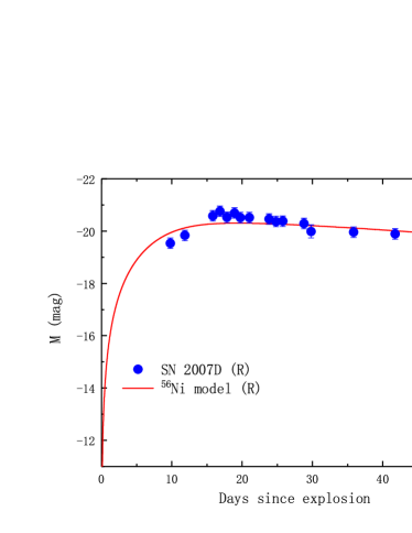
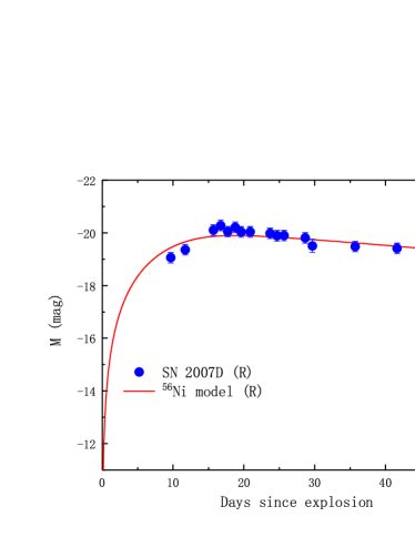
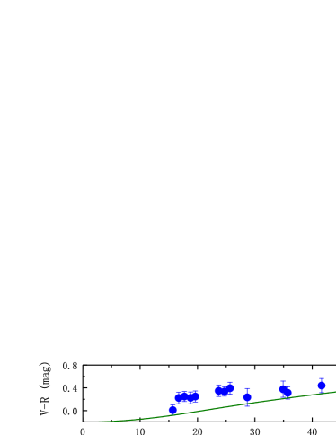
Figure 1.— The $R$-band LCs (top panels) and the color ($V-R$) evolution (bottom panels) reproduced by the ⁵⁶Ni model for Case A (left) and Case B (right). Data for Case A are taken from Drout et al. (2011). The abscissa represents time since the explosion in the rest frame.

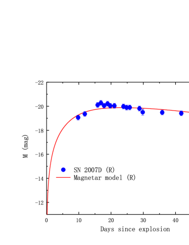
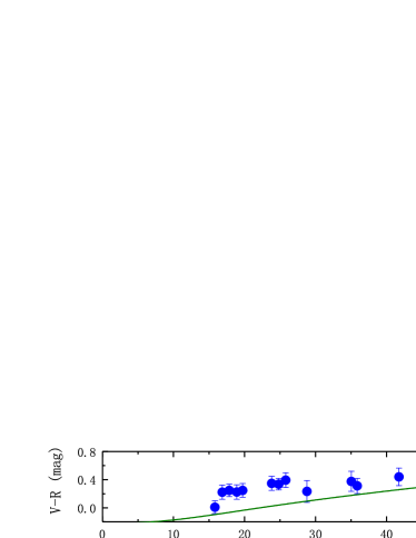
Figure 2.— The $R$-band LCs (top panels) and the $V-R$ color evolution (bottom panels) reproduced by the magnetar model for Case A (left) and Case B (right). Data for Case A are taken from Drout et al. (2011). The abscissa represents time since the explosion in the rest frame.

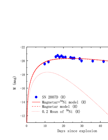
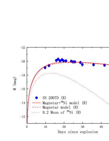
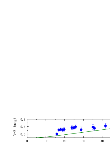
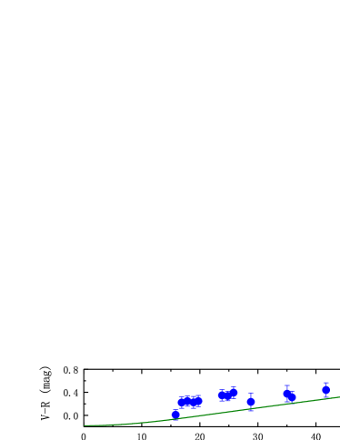
Figure 3.— The $R$-band LCs (top panels) and the $V-R$ color evolution (bottom panels) reproduced by the magnetar+⁵⁶Ni model for Case A (left) and Case B (right). The dashed and dotted lines represent the LCs of the components from magnetar and the 0.2 M_⊙ of ⁵⁶Ni, respectively. Data for Case A are taken from Drout et al. (2011). The abscissa represents time since the explosion in the rest frame.

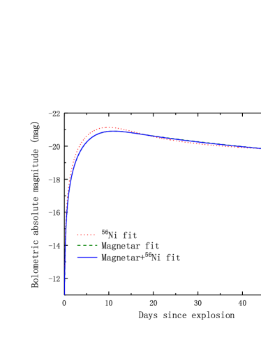
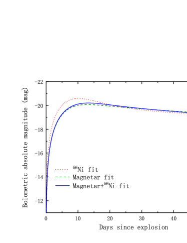
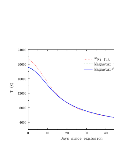
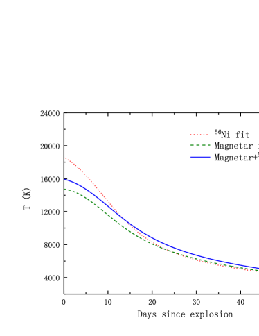
Figure 4.— The bolometric LCs (top panels) and the temperature evolution (bottom panels) reproduced by the ⁵⁶Ni model, the magnetar model, and the magnetar+⁵⁶Ni model for Case A (left panels) and Case B (right panels). The abscissa represents time since the explosion in the rest frame.

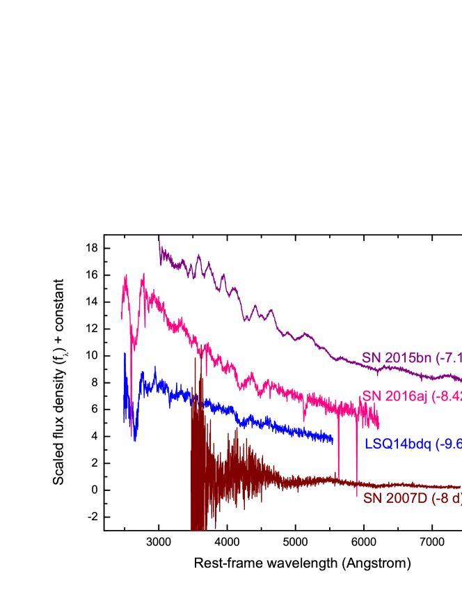
Figure 5.— Rest-frame premaximum spectra of SN 2007D and three SLSNe-I. The spectrum of SN 2007D was obtained from the CfA Supernova Archive (Modjaz et al., 2014) and corrected by taking the extinction ($E(B-V)=0.91+0.335=1.245$ mag) into account. Spectra of the other three SLSNe (LSQ14bdq, SN 2016aj, and SN 2015bn) were obtained from the Weizmann Interactive Supernova Data Repository (WISeREP) (Yaron & Gal-Yam, 2012), the Transient Name Server (https://wis-tns.weizmann.ac.il/), and Nicholl et al. (2016), respectively. The extinction-corrected spectrum of SN 2007D is cooler than that of these SLSNe-I, indicating that SN 2007D might be a luminous SN rather than a SLSN-I.

References

- Arcavi et al. (2016) Arcavi, I., Wolf, W. M., Howell, D. A., et al. 2016, ApJ, 819, 35
- Arnett (1982) Arnett, W. D. 1982, ApJ, 253, 785
- Bersten et al. (2016) Bersten, M. C., Benvenuto, O. G., Orellana, M., & Nomoto, K. 2016, ApJL, 817, L8
- Bessell et al. (1998) Bessell, M. S., Castelli, F., & Plez, B. 1998, A&A, 333, 231
- Cano et al. (2017) Cano, Z., Wang, S. Q., Dai, Z. G., Wu, X. F. 2017b, Advances in Astronomy, 8929054, 1
- Cappellaro et al. (1997) Cappellaro, E., Mazzali, P. A., Benetti, S., et al. 1997, A&A, 328, 203
- Chatzopoulos et al. (2012) Chatzopoulos, E., Wheeler, J. C., & Vinko, J. 2012, ApJ, 746, 121
- Chatzopoulos et al. (2013) Chatzopoulos, E., Wheeler, J. C., Vinko, J., et al. 2013a, ApJ, 773, 76
- Chen et al. (2017) Chen, K.-J., Moriya, T. J., Woosley, S., Sukhbold, T., Whalen, D. J., Suwa, Y., & Bromm, V. 2017, ApJ, 839, 85
- Chen et al. (2015) Chen, T.-W., Smartt, S. J., Jerkstrand, A., et al. 2015, MNRAS, 452, 1567
- Chevalier (1982) Chevalier, R. A. 1982, ApJ, 258, 790
- Chevalier & Fransson (1994) Chevalier, R. A., & Fransson, C. 1994, ApJ, 420, 268
- Chomiuk et al. (2011) Chomiuk, L., Chornock, R., Soderberg, A. M., et al. 2011, ApJ, 743, 114
- Chugai & Danziger (1994) Chugai, N. N., & Danziger, I. J. 1994, MNRAS, 268, 173
- Colgate & McKee (1969) Colgate, S. A., & McKee, C. 1969, ApJ, 157, 623
- Colgate et al. (1980) Colgate, S. A., Petschek, A. G., & Kriese, J. T. 1980, ApJL, 237, L81
- Dai et al. (2016) Dai, Z. G., Wang, S. Q., Wang, J. S., Wang, L. J., & Yu, Y. W. 2016, ApJ, 817, 132
- De Cia et al. (2018) De Cia, A., Gal-Yam, A., Rubin, A., et al. 2018, ApJ, 860, 100
- Dessart et al. (2012a) Dessart, L., Hillier, D. J., Li, C., & Woosley, S. 2012a, MNRAS, 424, 2139
- Dessart et al. (2012b) Dessart, L., Hillier, D. J., Waldman, R., Livne, E., & Blondin, S. 2012b, MNRAS, 426, L76
- Drout et al. (2011) Drout, M. R., Soderberg, A. M., Gal-Yam, A., et al. 2011, ApJ, 741, 97
- Filippenko (1997) Filippenko, A. V. 1997, ARA&A, 35, 309
- Filippenko et al. (1995) Filippenko, A. V., Barth, A. J., Matheson, T., et al. 1995, ApJ, 450, L11
- Gal-Yam (2012) Gal-Yam, A. 2012, Science, 337, 927
- Gal-Yam (2018) Gal-Yam, A. 2018, arXiv:1812.01428
- Gal-Yam (2017) Gal-Yam, A. 2017, Observational and Physical Classification of Supernovae. In: Alsabti A., Murdin P. (eds) Handbook of Supernovae. Springer, 2017, p. 195 (arXiv:1611.09353)
- Ginzburg & Balberg (2012) Ginzburg, S., & Balberg, S. 2012, ApJ, 757, 178
- Hjorth & Bloom (2012) Hjorth, J., & Bloom, J. S. 2012, in Chapter 9 in Gamma-Ray Bursts, ed. C. Kouveliotou, R. A. M. J. Wijers, & S. Woosley (Cambridge Astrophysics Series, Vol. 51; Cambridge: Cambridge Univ. Press), 169
- Inserra et al. (2013) Inserra, C., Smartt, S. J., Jerkstrand, A., et al. 2013, ApJ, 770, 128
- Iwamoto et al. (1998) Iwamoto, K., Mazzali, P. A., Nomoto, K., et al. 1998, Nature, 395, 672
- Iwamoto et al. (1994) Iwamoto, K., Nomoto, K., Höflich, P., Yamaoka, H., Kumagai, S., & Shigeyama, T., 1994, ApJL, 437, L115
- Janka et al. (2016) Janka, H.-T., Melson, T., & Summa, A. 2016, ARNPS, 66, 341
- Kasen & Bildsten (2010) Kasen, D., & Bildsten, L. 2010, ApJ, 717, 245
- Li et al. (2011) Li, W., Leaman, J., Chornock, R., et al. 2011, MNRAS, 412, 1441
- Liu et al. (2018) Liu, L. D., Wang, L. J., Wang, S. Q., & Dai, Z. G. 2018, ApJ, 856, 59
- Liu et al. (2017a) Liu, L. D., Wang, S. Q., Wang, L. J., Dai, Z. G., Yu, H., & Peng, Z. K. 2017a, ApJ, 842, 26
- Liu et al. (2017b) Liu, Y. Q., Modjaz, M., & Bianco, F. B. 2017b, ApJ, 845, 85
- Maeda et al. (2003) Maeda, K., Mazzali, P. A., Deng, J., Nomoto, K., Yoshii, Y., Tomita, H., & Kobayashi, Y. 2003, ApJ, 593, 931
- Maeda et al. (2007) Maeda, K., Tanaka, M., Nomoto, K., Tominaga, N., Kawabata, K., Mazzali, P. A., Umeda, H., Suzuki, T., & Hattori, T. 2007, ApJ, 666, 1069
- Matheson et al. (2001) Matheson, T., Filippenko, A. V., Li W., Leonard, D. C., & Shields, J. C., 2001, AJ, 121, 1648
- Mazzali et al. (2000) Mazzali, P. A., Iwamoto, K., & Nomoto, K. 2000, ApJ, 545, 407
- Metzger et al. (2015) Metzger, B. D., Margalit, B., Kasen, D., & Quataert, E. 2015, MNRAS, 454, 3311
- Modjaz et al. (2014) Modjaz, M., Blondin, S., Kirshner, R. P., et al. 2014, AJ, 147, 99
- Modjaz et al. (2016) Modjaz, M., Liu, Y. Q., Bianco, F. B., & Graur, O. 2016, ApJ, 832, 108
- Nagy & Vinkó (2016) Nagy, A. P., & Vinkó, J. 2016, A&A, 589, 53
- Nicholl et al. (2016) Nicholl, M., Berger, E., Smartt, S. J., et al. 2016, ApJ, 826, 39
- Nicholl et al. (2017) Nicholl, M., Guillochon, J., & Berger, E. 2017, ApJ, 850, 55
- Nicholl et al. (2015) Nicholl, M., Smartt, S. J., Jerkstrand, A., et al. 2015, MNRAS, 452, 3869
- Nomoto et al. (2013) Nomoto, K., Kobayashi, C., & Tominaga, N. 2013, ARA&A, 51, 457
- Nomoto et al. (1994) Nomoto, K., Yamaoka, H., Pols, O. R., van den Heuvel, E. P. J., Iwamoto, K., Kumagai, S., & Shigeyama, T., 1994, Nature, 371, 227
- Nugent et al. (2006) Nugent, P. E., Sullivan, M., Ellis, R., et al. 2006, ApJ, 645, 841
- Quimby (2014) Quimby, R. M. 2014, IAUS, 296, 68
- Quimby et al. (2018) Quimby, R. M., De Cia, A., Gal-Yam, A., et al. 2018, ApJ, 855, 2
- Quimby et al. (2011) Quimby, R. M., Kulkarni, S. R., Kasliwal, M. M., et al. 2011, Nature, 474, 487
- Sauer et al. (2006) Sauer, D. N., Mazzali, P. A., Deng, J., Valenti, S., Nomoto, K., & Filippenko, A. V. 2006, MNRAS, 369, 1939
- Schlafly & Finkbeiner (2011) Schlafly, E. F., & Finkbeiner, D. P. 2011, ApJ, 737, 103
- Schlegel et al. (1998) Schlegel, D. J., Finkbeiner, D. P., & Davis, M. 1998, ApJ, 500, 525
- Umeda & Nomoto (2008) Umeda, H., & Nomoto, K. 2008, ApJ, 673, 1014
- Wang et al. (2017a) Wang, L. J., Cano, Z., Wang, S. Q., et al. 2017a, ApJ, 851, 54
- Wang et al. (2016a) Wang, L. J., Han, Y. H., Xu, D., et al. 2016a, ApJ, 831, 41
- Wang et al. (2016b) Wang, L. J., Wang, S. Q., Dai, Z. G., Xu, D., Han, Y. H., Wu, X. F., & Wei, J. Y. 2016b, ApJ, 821, 22
- Wang et al. (2017b) Wang, L. J., Yu, H., Liu, L. D., Wang, S. Q., Han, Y. H., Xu, D., Dai, Z. G., Qiu, Y. L., & Wei, J. Y. 2017b, ApJ, 837, 128
- Wang et al. (2017c) Wang, S. Q., Cano, Z., Wang, L. J., Zheng, W., Dai, Z. G., Filippenko, A. V., & Liu, L. D. 2017c, ApJ, 850, 148
- Wang et al. (2015a) Wang, S. Q., Wang, L. J., Dai, Z. G., & Wu, X. F. 2015a, ApJ, 799, 107
- Wang et al. (2015b) Wang, S. Q., Wang, L. J., Dai, Z. G., & Wu, X. F. 2015b, ApJ, 807, 147
- Wegner et al. (1993) Wegner, G., Haynes, M. P., & Giovanelli, R. 1993, AJ, 105, 1251
- Woosley (2010) Woosley, S. E. 2010, ApJL, 719, L204
- Woosley & Bloom (2006) Woosley, S. E., & Bloom, J. S. 2006, ARA&A, 44, 507
- Yaron & Gal-Yam (2012) Yaron, O., & Gal-Yam, A. 2012, PASP, 124, 668
- Yu et al. (2017) Yu, Y. W., Zhu, J. P., Li, S. Z., Lü, H. J., & Zou, Y. C. 2017, ApJ, 840, 12