Robust Network Design for Software-Defined IP/Optical Backbones

Abstract

Recently, Internet service providers (ISPs) have gained increased flexibility in how they configure their in-ground optical fiber into an IP network. This greater control has been made possible by (i) the maturation of software defined networking (SDN), and (ii) improvements in optical switching technology. Whereas traditionally, at network design time, each IP link was assigned a fixed optical path and bandwidth, modern colorless and directionless Reconfigurable Optical Add/Drop Multiplexers (CD ROADMs) allow a remote SDN controller to remap the IP topology to the optical underlay on the fly. Consequently, ISPs face new opportunities and challenges in the design and operation of their backbone networks [1, 2, 3, 4].

Specifically, ISPs must determine how best to design their networks to take advantage of the new capabilities; they need an automated way to generate the least expensive network design that still delivers all offered traffic, even in the presence of equipment failures. This problem is difficult because of the physical constraints governing the placement of optical regenerators, a piece of optical equipment necessary for maintaining an optical signal over long stretches of fiber. As a solution, we present an integer linear program (ILP) which (1) solves the equipment-placement network design problem; (2) determines the optimal mapping of IP links to the optical infrastructure for any given failure scenario; and (3) determines how best to route the offered traffic over the IP topology. To scale to larger networks, we also describe an efficient heuristic that finds nearly optimal network designs in a fraction of the time. Further, in our experiments our ILP offers cost savings of up to 29% compared to traditional network design techniques.

I Introduction

Over the past several years, the advent of software defined networking (SDN), along with improvements in optical switching technology, has given network operators more flexibility in configuring their in-ground optical fiber into an IP network. Whereas traditionally, at network design time, each IP link was assigned a fixed optical path and bandwidth, modern SDN controllers can program colorless and directionless Reconfigurable Optical Add/Drop Multiplexers (CD ROADMs) to remap the IP topology to the optical underlay on the fly, while the network continues carrying traffic and without deploying technicians to remote sites (Figure 1) [1, 2, 3, 4].

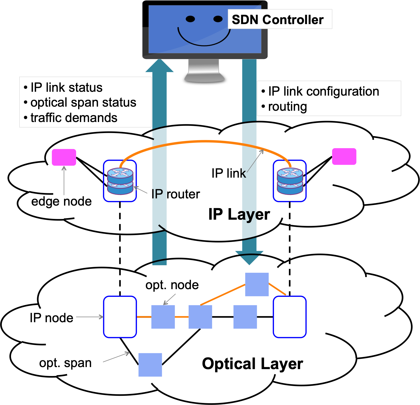
Figure 1: Layered IP/optical architecture. The highlighted orange optical spans comprise one possible mapping of the orange IP link to the optical layer. Alternatively, the SDN controller could remap the same orange IP link to follow the black optical path.

In the traditional setting, if a router failure or fiber cut causes an IP link to go down, all resources that were being used for said IP link are rendered useless. There are two viable strategies to recover from any single optical span or IP router failure. First, we could independently restore the optical and IP layers, depending on the specific failure; we could perform pure optical recovery in the case of an optical span failure or pure IP recovery in the case of an IP router failure. Note that the strategy we refer to as “pure optical recovery” of course involves reestablishing the IP link over the new optical path. We call it “pure optical recovery” because once the link has been recreated over the new optical path, the change is transparent to the IP layer. Second, we could design the network with sufficient capacity and path diversity that we can at runtime perform pure IP restoration. In practice, ISPs have used the latter strategy, as it is generally more resource efficient [5].

Now, the optical and electrical equipment can be repurposed for setting up the same IP link along a different path, or even for setting up a different IP link. In the context of failure recovery, the important upshot is that joint multilayer (IP and optical) failure recovery is now possible at runtime. The SDN controller is responsible for performing this remote reprogramming of both CD ROADMs and routers; while we generally think of SDN as operating at the network layer and above, it is now extending into the physical layer.

Thus, SDN-enabled CD ROADMs shift the boundary between network design and network operation (Figure 2). We use the term network design to refer to any changes that happen on a human timescale, e.g., installing new routers or dispatching a crew to fix a failed link. We use network operation to refer to changes that can happen on a smaller timescale, e.g., adjusting routing in response to switch or link failures or changing demands.

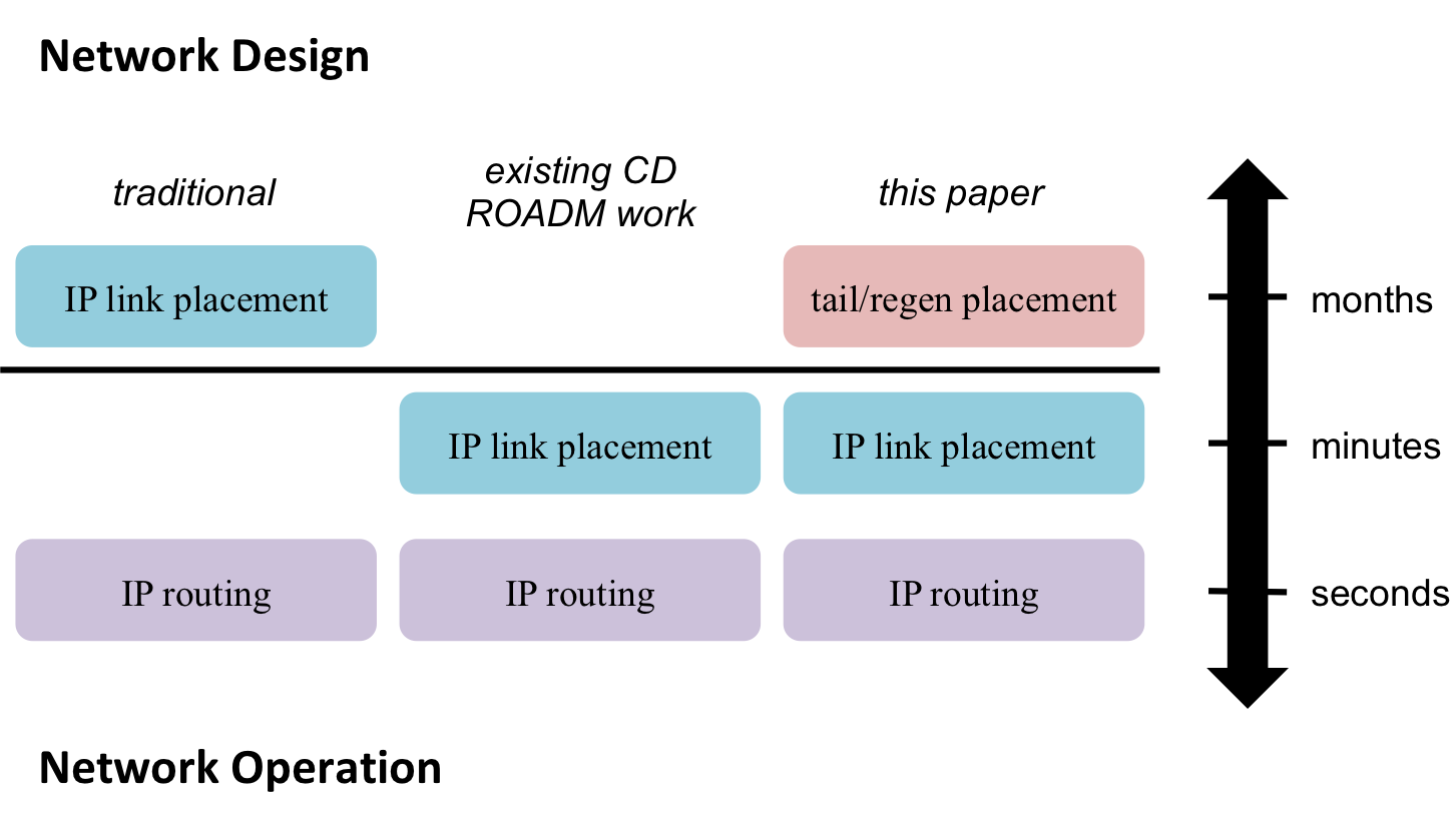
Figure 2: Components of network design vs. network operation in, from left to right: traditional networks, existing studies on how best to take advantage of CD ROADMs, and this paper. The vertical dimension is timescale.

As Figure 2 shows, network design used to comprise IP link placement. To describe what it now entails, we must provide background on IP/optical backbone architecture (Figure 3). The limiting resources in the design of an IP backbone are the equipment housed at each IP and optical-only node. Specifically, an IP node’s responsibility is to terminate optical links and convert the optical signal to an electrical signal, and to do so it needs enough tails (tail is shorthand for the combination of an optical transponder and a router port). An optical node must maintain the optical signal over long distances, and to do so it needs enough regenerators or regens for the IP links passing through it. Therefore, we precisely state the new network design problem as follows: Place tails and regens in a manner that minimizes cost while allowing the network to carry all expected traffic, even in the presence of equipment failures.

This new paradigm creates both new opportunities and challenges in the design and operation of backbone networks [6]. Previous work has explored the advantages of joint multilayer optimization over traditional IP-only optimization [1, 2, 3, 4] (e.g., see Table 1 of [3]). However, these authors primarily resorted to heuristic optimization and restoration algorithms, due to the restrictions of routing (avoiding splitting flows into arbitrary proportions), the need for different restoration and latency guarantees for different quality-of-service classes, and the desirability of fast run times.

Further complicating matters is that network components fail, and when they do a production backbone must reestablish connectivity within seconds. Tails and regens cannot be purchased or relocated at this timescale, and therefore our network design must be robust to a set of possible failure scenarios. Importantly, we consider as failure scenarios any single optical fiber cut or IP router failure. There are other possible causes of failure (e.g., single IP router port, ROADM, transponder, power failure), which allow for various alternative recovery techniques, but we focus on these two. Existing techniques respond efficiently to IP layer failures [6] or optical layer failures, but ours is the first to jointly optimize over the two.

Thus, we overcome three main challenges to present an exact formulation and solution to the network design problem.

1. The solution must be a single tail and regen configuration that works for all single IP router and optical fiber failures. This configuration should minimize cost under the assumption that the IP link topology will be reconfigured in response to each failure.

2. The positions of regens relative to each other along the optical path determine which IP links are possible.

3. The problem is computationally complex because it requires integer variables and constraints. Each tail and each regen supports a 100 Gbps IP link. Multiple tails or multiple regens can be combined at a single location to build a faster link, but they can’t be split into e.g., 25 Gbps units that cost 25% of a full element.

These challenges arise because the recent shift in the boundary between network design and operation fundamentally changes the design problem; simply including link placement in network operation optimizations does not suffice to fully take advantage of CD ROADMs. A network design is optimal relative to a certain set of assumptions about what can be reconfigured at runtime. Hence, traditional network designs are only optimal under the assumption that tails and regens are fixed to their assigned IP links. With CD ROADMs, the optimal network design must be computed under the assumption that IP links will be adjusted in response to failures or changing traffic demands.

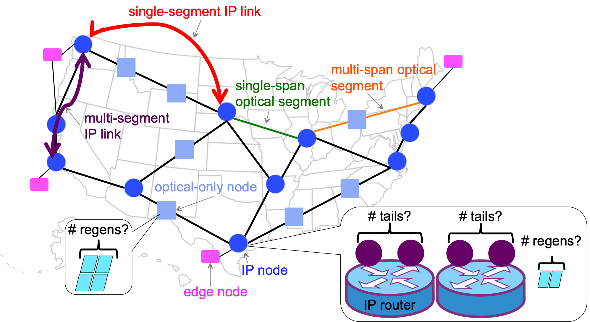
Figure 3: IP/optical network terminology.

To this end, we make three main contributions.

1. After describing the importance of jointly optimizing over the IP and optical layers in Section II, we formulate the optimal network design algorithm (Section III). In this way we address challenges (1) and (2) from above.

2. We present two scalable, time-efficient approximation algorithms for the network design problem, addressing the computational complexity introduced by the integer constraints (Section IV), and we explain which use cases are best suited to each of our algorithms (Section IV-C).

3. We evaluate our three algorithms in relation to each other and to legacy networks (Section V).

We discuss related work in Section VI and conclude in Section VII.

II IP/Optical Failure Recovery

In this section we provide more background IP/optical networks. We begin by defining key terms and introducing a running example (Section II-A). We then use this example to discuss various failure recovery options in both traditional (Section II-B) and CD ROADM (Section II-C) IP/optical networks.

II-A IP/Optical Network Architecture

As shown in Figure 3, an IP/optical network consists of optical fiber, the IP nodes where fibers meet, the optical nodes stationed intermittently along fiber segments, and the edge nodes that serve as the sources and destinations of traffic. We do not consider the links connecting an edge router to a core IP router as part of our design problem; we assume these are already placed and fault tolerant.

Each IP node houses one or more IP routers, each with zero or more tails, and zero or more optical regens. Each optical-only node houses zero or more optical regens but cannot contain any routers (Figure 3). While IP and optical nodes serve as the endpoints of optical spans and segments, specific IP routers serve as the endpoints of IP links.

For our purposes, an optical span is the smallest unit describing a stretch of optical fiber; an optical span is the section of fiber between any two nodes, be they IP or optical-only. Optical-only nodes can join multiple optical spans into a single optical segment, which is a stretch of fiber terminated at both ends by IP nodes. The path of a single optical segment may contain one or more optical-only nodes. The physical layer underlying each IP link comprises one or more optical segments. An IP link is terminated at each end by a specific IP router and can travel over multiple optical segments if its path traverses an intermediate IP node without terminating at one of that node’s routers. Figure 3 illustrates the roles of optical spans and segments and IP links. The locations of all nodes and optical spans are fixed and cannot be changed, either at design time or during network operation.

An optical signal can travel only a finite distance along the fiber before it must be regenerated; every regen_dist miles the optical signal must pass through a regen, where it is converted from an optical signal to an electrical signal and then back to optical before being sent out the other end. The exact value of regen_dist varies depending on the specific optical components, but it is roughly 1000 miles for our setting of a long-distance ISP backbone with 100 Gbps technology. We use the value of $\texttt{\sc regen\_dist}=1000$ miles throughout this paper.

Example network design problem. The network in Figure 4 has two IP nodes, $\mathcal{I}$1 and $\mathcal{I}$2, and five optical-only nodes, O1-O5. $\mathcal{I}$1 and $\mathcal{I}$2 each have two IP routers (I1, I2 and I3, I4, respectively). Edge routers E1 and E2 are the sources and destinations of all traffic. The problem is to design the optimal IP network, requiring the fewest tails and regens, to carry 80 Gbps from E1 to E2 while surviving any single optical span or IP router failure. We do not consider failures of E1 or E2, because failing the source or destination would render the problem trivial or impossible, respectively.

If we don’t need to be robust to any failures, the optimal solution is to add one 100 Gbps IP link from I1 to I3 over the nodes $\mathcal{I}$1, O1, O2, O3, and $\mathcal{I}$2. This solution requires one tail each at I1 and I3 and one regen at O2, for a total of two tails and one regen.

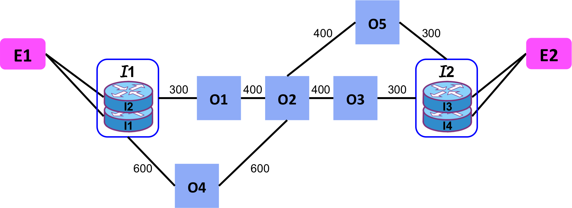
Figure 4: Example optical network illustrating the different options for failure restoration. The number near each edge is the edge’s length in miles.

II-B Failure Recovery in Traditional Networks

In the traditional setting, the design problem is to place IP links; in this setting, once an IP link is placed at design time, its tails and regens are permanently committed to it. If one optical span or router fails, the entire IP link fails and the rest of its resources lie idle. During network operation, we may only adjust routing over the established IP links.

In general, this setup allows for four possible types of failure restoration. Two of these techniques are inadequate because they cannot recover from all relevant failure scenarios (first two rows of Table I). The other two are effective but suboptimal in their resource requirements (second two rows of Table I). We describe these four approaches below, guided by the running example shown in Figure 4. In Section II-C we show that CD ROADMs allow for a network design that meets our problem’s requirements in a more cost-effective way.

TABLE I: Properties of various failure recovery approaches. The first four techniques are possible in legacy and CD ROADM networks, while the fifth requires CD ROADMs.

Recovery Technique	# Tails	# Regens	IP?	Optical?
pure optical	2	2	✗	✔
pure IP, shortest path	4	4	✔	✗
pure IP, any path	4	3	✔	✔
separate IP and optical	4	4	✔	✔
joint IP/optical	4	2	✔	✔

Inadequate recovery techniques. In pure optical layer restoration, if an optical span fails, we reroute each affected IP link over the optical network by avoiding the failed span. The rerouted path may require additional regens. In the example shown in Figure 4, this amounts to rerouting the IP link along the alternate path $\mathcal{I}$1-O4-O2-O5-$\mathcal{I}$2 whenever any optical span fails. This path requires one regen each at O4 and O2. However, because the ($\mathcal{I}$1, $\mathcal{I}$2) link will never be instantiated over both paths simultaneously, the second path can reuse the original regen O2. Hence, we need only buy one extra regen at O4, for a total of two tails (at $\mathcal{I}$1 and $\mathcal{I}$2) and two regens (at O2 and O4). The problem with this pure optical restoration strategy is that it cannot protect against IP router failures.

In pure IP layer restoration with each IP link routed along its shortest optical path, we maintain enough fixed IP links such that during any failure condition, the surviving IP links can carry the required traffic. If any component of an IP link fails, then the entire IP link fails and even the intact components cannot be used. In large networks, this policy usually finds a feasible solution to protect against any single router or optical span failure. However, it may not be optimally cost-effective due to the restriction that IP links follow the shortest optical paths. Furthermore, in small networks it may not provide a solution that is robust to all optical span failures.

If we only care about IP layer failures, the optimal strategy for our running example is to place two 100 Gbps links, one from I1 to I3 and a second from I2 to I4 and both following the optical path $\mathcal{I}$1-O1-O2-O3-$\mathcal{I}$2. Though this design is robust to the failure of any one of I1, I2, I3, and I4, it cannot protect against optical span failures.

Correct but suboptimal recovery techniques. In contrast to the two failure recovery mechanisms described above, the following two techniques can correctly recover from any single IP router or optical span failure. However, neither reliably produces the least expensive network design.

Pure IP layer restoration with no restriction on how IP links are routed over the optical network is the same as IP restoration over shortest paths except IP links can be routed over any optical path. With this policy, we always find a feasible solution for all failure conditions, and it finds the most cost-effective among the possible pure-IP solutions. However, its solutions still require more tails or regens than those produced by our ILP, and solving for this case is computationally complex. In terms of Figure 4, pure IP restoration with no restriction on IP links’ optical paths entails routing the (I1, I3) IP link along the $\mathcal{I}$1-O1-O2-O3-$\mathcal{I}$2 path and the (I2, I4) IP link along the $\mathcal{I}$1-O4-O2-O5-$\mathcal{I}$2 path. This requires two tails plus one regen (at O2) for the first IP link and two tails plus two regens (at O4 and O2) for the second IP link, for a total of four tails and three regens.

The final failure recovery technique possible in legacy networks, without CD ROADMs, is pure IP layer restoration for router failures and pure optical layer restoration for optical failures. This policy works in all cases but is usually more expensive than the two pure IP layer restorations mentioned above. In terms of our running example, we need two tails and two regens for each of two IP links, as we showed in our discussion of pure IP recovery along shortest paths. Hence, this strategy requires a total of four tails and four regens.

In summary, the optimal network design with legacy technology that is robust to optical and IP failures requires four tails and three regens.

II-C Failure Recovery in CD ROADM Networks

A modern IP/optical network architecture is identical to that described in Section II-A aside from the presence of an SDN controller. This single logical controller receives notifications of the changing status of any IP or optical component and also any changes in traffic demands between any pair of edge routers and uses this information compute the optimal IP link configuration and the optimal routing of traffic over these links. It then communicates the relevant link configuration instructions to the CD ROADMs and the relevant forwarding table changes to the IP routers.

As in the traditional setting, we cannot add or remove edge nodes, IP nodes, optical-only nodes, or optical fiber. But, now the design problem is to decide how many tails to place on each router and how many regens to place at each IP and optical node; no longer must we commit to fixed IP links at design time. Routing remains a key component of the network design problem, though it is now joined by IP link placement.

Any of the four existing failure recovery techniques is possible in a modern network. In addition, the presence of SDN-controlled CD ROADMs allows for a fifth option, joint IP/optical recovery. In contrast to the traditional setting, IP links can now be reconfigured at runtime. As above, suppose the design calls for an IP link between routers $\mathcal{I}$1 and $\mathcal{I}$2 over the optical path I1-I2-I3-I4. Now, these resources are not permanently committed this IP link. If one component fails, the remaining tails and regens can be repurposed either to reroute the ($\mathcal{I}$1, $\mathcal{I}$2) link over a different optical path or to (help) establish an entirely new IP link.

Returning to our running example, with joint IP/optical restoration, we can recover from any single IP or optical failure with just one IP link from I1 to I3. If there is any optical link failure then this link shifts from its original shortest path, which needs a regen at O2, to the path $\mathcal{I}$1-O4-O2-O5-$\mathcal{I}$2, which needs regens at O2 and O4. Importantly, the regen at O2 can be reused. Hence, thus far we need two tails and two regens. To account for the possibility of I1 failing, we add an extra tail at I2; if I1 fails then at runtime we create an IP link from I2 to I3 over the path $\mathcal{I}$1-O1-O2-O3-$\mathcal{I}$2. Since this link is only active in the case that I1 has failed, it will never be instantiated at the same time as the (I1, I3) link and can therefore reuse the regen we already placed at O2. Finally, to account for the possibility of I3 failing, we add an extra tail at I4. This way, at runtime we can create the IP link (I1, I4) along the path $\mathcal{I}$1-O1-O2-O3-$\mathcal{I}$2. Again, only one of these IP links will ever be active at one time, so we can reuse the regen at O2. Therefore, our final joint optimization design requires four tails and two regens. Hence, even in this simple topology, compared to the most cost efficient traditional strategy, joint IP/optical optimization and failure recovery saves the cost of one regen.

II-C1 A note on transient disruptions

As shown in Figure 2, IP link configuration operates on the order of minutes, while routing operates on sub-second timescales. IP link configuration takes several minutes because the process entails the following three steps:

1. Adding or dropping certain wavelengths at certain ROADMs;

2. Waiting for the network to return to a stable state; and

3. Ensuring that the network is indeed stable.

A “stable state” is one in which the optical signal reaches tails at IP link endpoints with sufficient optical power to be correctly converted back into an electrical signal. Adding or dropping wavelengths at ROADMs temporarily reduces the signal’s power enough to interfere with this optical-electrical conversion, thereby rendering the network temporarily unstable. Usually, the network correctly returns to a stable state within seconds of reprogramming the wavelengths (i.e., steps (1) and (2) finish within seconds). However, to ensure that the network is always operating with a stable physical layer (step (3)), manufacturers add a series of tests and adjustments to the reconfiguration procedure. These tests take several minutes, and therefore step (3) delays completion of the entire process. Researchers are currently working to bring reconfiguration latency down to the order of milliseconds [7], similar to the timescale at which routing currently operates. However, for now we must account for a transition period of approximately two minutes when the link configuration has not yet been updated and is therefore not optimal for the new failure scenario.

During this transient period, the network may not be able to deliver all the offered traffic. We mitigate this harmful traffic loss by immediately reoptimizing routing over the existing topology while the network is transitioning to its new configuration. As we show in Section V-D, by doing so we successfully deliver the vast majority of offered traffic under almost all failure scenarios. Many operational ISPs carry multiple classes of traffic, and their service level agreements (SLAs) allow them to drop some low priority traffic under failure or extreme congestion. At one large ISP, approximately 40-60% of traffic is low priority. We always deliver at least 50% of traffic just by rerouting.

III Network Design Problem

We now describe the variables and constraints of our integer linear program (ILP) for solving the network design problem. After formally stating the objective function in Section III-A we introduce the problem’s constraints in III-B and III-C. To avoid cluttering our presentation of the main ideas of the model, throughout III-A - III-C we assume exactly one router per IP node. In III-D we relax this assumption, and we also explain how to extend the model to changing traffic demands.

For ease of explanation, we elide the distinction between edge nodes and IP nodes; we treat IP nodes as the ultimate sources and destinations of traffic.

III-A Minimizing Network Cost

Our inputs are (i) the optical topology, consisting of the set $\mathcal{I}$ of IP nodes, the set $O$ of optical nodes, and the fiber links (annotated with distances) between them; and (ii) the demand matrix $D$.

We use the variable $T_{u}$ to represent the number of tails that should be placed at router $u$, and $R_{u}$ represents the number of regens at node $u$. An optical-only node can’t have any tails.

The capacity of an IP link $\ell=(\alpha,\beta)$ is limited by the number of tails dedicated to $\ell$ at $\alpha$ and $\beta$ and the number of regens dedicated to $\ell$. Technically, the original signal emitted by $\alpha$ is strong enough to travel regen_dist, and $\ell$ doesn’t need regens there. However, for ease of explanation, we assume that $\ell$ does need regens at $\alpha$, regardless of its length. This requirement of regens at the beginning of each IP link is necessary only for the mathematical model and not in the actual network. We add a trivial postprocessing step to remove these regens from the final count before reporting our results. Table II summarizes our notation.

TABLE II: Notation.

		Definition
Inputs	$\mathcal{I}$	set of IP nodes
	$I$	set of IP routers
	$O$	set of optical-only nodes
	$N$	set of all nodes ($N=\mathcal{I}\cup O$)
	$D$	demand matrix, where $D_{st}\in D$ gives the demand from IP node $s$ to IP node $t$
	$F$	set of all possible failure scenarios $F=\{f_{1},f_{2},\dots,f_{n}\}$
	$dist_{uvf}$	shortest distance from optical node $u$ to optical node $v$ in failure scenario $f$
	$O_{uf}$	set of all next-hops $v$ with $dist_{uvf}<\texttt{\sc regen\_dist}$
Outputs	$T_{u}$	number of tails placed at IP router $u$
(Network Design)	$R_{u}$	total regens placed at optical node $u$
Outputs	$X_{\alpha\beta f}$	capacity of IP link $(\alpha,\beta)$ in failure scenario $f$
(Network Operation)	$Y_{st\alpha\beta f}$	amount of $(s,t)$ traffic routed on IP link $(\alpha,\beta)$ in failure scenario $f$
Intermediate	$R_{\alpha\beta uvf}$	number of regens at $u$ for optical segment $(u,v)$ of IP link $(\alpha,\beta)$ in failure $f$
Values	$R_{uf}$	number of regens needed at optical node $u$ in failure scenario $f$

Our objective is to place tails and regens to minimize the ISP’s equipment costs while ensuring that the network can carry all necessary traffic under all failure scenarios. Let $c_{T}$ and $c_{R}$ be the cost of one tail and one regen, respectively. Then the total cost of all tails is $c_{T}\sum_{u\in I}T_{u}$, the total cost of all regens is $c_{R}\sum_{u\in O}R_{u}$, and our objective is

$$\min~{}~{}c_{T}\sum_{u\in I}T_{u}+c_{R}\sum_{u\in O}R_{u}.$$

The stipulation that the output tail and regen placement work for all failure scenarios is crucial. Without some dynamism in the inputs, be it from a changing topology across failure scenarios or from a changing demand matrix, CD ROADMs’ flexible reconfigurability would be useless. We focus on robustness to IP router and optical span failures because conversations with one large ISP indicate that failures affect network conditions more than routine demand fluctuations. Extending our model to find a placement robust to both equipment failures and changing demands should be straightforward.

III-B Robust Placement of Tails and Regens

In traditional networks, robust design requires choosing a single IP link configuration that is optimal for all failure scenarios under the assumption that routing will depend on the specific failure state [6]. With CD ROADMs, robust network design requires choosing a single tail/regen placement that is optimal for all failure scenarios under the assumption that both routing and the IP topology will depend on the specific failure state. In either case, solving the network design problem requires solving the network operation problem as an “inner loop”; to determine the optimal network design we need to simulate how a candidate network would operate, in terms of IP link placement and routing, in each failure scenario.

At the mathematical level, CD ROADMs introduce two additional sets of decision variables to the traditional network design optimization. With the old technology, the problem is to optimize over two sets of decision variables: one set for where to place IP links and what the capacities of those links should be, and a second set for which links different volumes of traffic should traverse. In traditional network design, there is no need to explicitly model tails and regens separate from link placement, because each tail or regen is associated with exactly one IP link. Now, any given tail or regen is not associated with exactly one IP link. Thus, we must decide not only link placement and routing but also the number of tails to place at each IP node and the number of regens to place at each site. We describe these two novel aspects of our formulation in turn.

Constraints governing tail placement. Our first constraint requires that the number of tails placed at any router $u$ is enough to accommodate all the IP links $u$ terminates:

$$\sum_{\alpha\in I}X_{\alpha uf} \leq T_{u}$$ (1)

$$\sum_{\beta\in I}X_{u\beta f} \leq T_{u}$$

$$\forall u\in I,\forall f\in F$$

As shown in Table II, $X_{\alpha uf}$ is the capacity of IP link $(\alpha,u)$ in failure scenario $f$. Hence, $\sum_{\alpha\in I}X_{\alpha uf}$ is the total incoming bandwidth terminating at router $u$, and Constraint (1) says that $u$ needs at least this number of tails. Analogously, $\sum_{\beta\in I}X_{u\beta f}$ is the total outgoing bandwidth from $u$, and Constraint (III-B) ensures that $u$ has enough tails for these links, too. We don’t need $T_{u}$ greater than the sum of these quantities because each tail supports a bidirectional link.

Constraints governing regen placement. The second fundamental difference between our model and existing work is that we must account for relative positioning of regens both within and across failure scenarios. Because of physical limitations in the distance an optical signal can travel, no IP link can include a span longer than regen_dist without passing through a regenerator. As a result, the decision to place a regen at one optical location depends on the decisions we make about other locations, both within a single failure scenario and across changing network conditions. Therefore, we introduce auxiliary variables $R_{\alpha\beta uvf}$ to represent the number of regens to place at node $u$ for the link between IP routers $(\alpha,\beta)$ in failure scenario $f$ such that the next regen traversed will be at node $v$.

Ultimately, we want to solve for $R_{u}$, the number of regens to place at $u$, which doesn’t depend on the IP link, next-hop regen, or failure scenario. But, we need the $R_{\alpha\beta uvf}$ variables to encode these dependencies in our constraints. We connect $R_{u}$ to $R_{\alpha\beta uvf}$ with the constraint

$$R_{u}\geq\sum_{\begin{subarray}{c}\alpha,\beta\in I\\ v\in O\end{subarray}}R_{\alpha\beta uvf}~{}~{}\forall u\in O,\forall f\in F.$$ (3)

We use four additional constraints for the $R_{\alpha\beta uvf}$ variables. First, we prevent some node $v$ from being the next-hop regen for some node $u$ if the shortest path between $u$ and $v$ exceeds regen_dist:

$$R_{\alpha\beta uvf} = 0$$

$$\forall\alpha,\beta\in I,$$

$$\forall u,v~{}\text{such that}~{}dist_{uvf}>\texttt{\sc regen\_dist}.$$

Second, we ensure that the set of regens assigned to an IP link indeed forms a contiguous path. That is, for all nodes $u$ aside from those housing the source and destination routers, the number of regens assigned to $u$ equals the number of regens for which $u$ is the next-hop:

$$\sum_{v\in N}R_{\alpha\beta uvf} = \sum_{v\in N}R_{\alpha\beta vuf}$$

$$\forall u\in N,\forall\alpha,\beta\in I,\forall f\in F.$$

We need sufficient regens at the source IP router’s node $a$, and sufficient regens with the destination IP router’s node $b$ as their next-hop, for each IP link

$$\sum_{u\in N}R_{\alpha\beta auf} \geq X_{\alpha\beta f}$$

$$\sum_{u\in N}R_{\alpha\beta ubf} \geq X_{\alpha\beta f}$$

$$\forall\alpha,\beta\in I,\forall f\in F;$$

But, $b$ can’t have any regens, and $a$ can’t be the next-hop location for any regens

$$R_{\alpha\beta uaf}=R_{\alpha\beta buf}=0$$

$\forall u\in N,\forall\alpha,\beta\in I,\forall f\in F.$

Additional practical constraints. We have two practical constraints which are not fundamental to the general problem but are artifacts of the current state of routing technology. First, ISPs build IP links in bandwidths that are multiples of 100 Gbps. We encode this policy by requiring $X_{\alpha\beta f}$, $T_{u}$, and $R_{u}$ to be integers and converting our demand matrix into 100 Gbps units.

Second, current IP and optical equipment require each IP link to have equal capacity to its opposite direction. With these constraints, only one of (1) and (III-B) is necessary.

Finally, we require all variables to take on nonnegative values.

III-C Dynamic Placement of IP Links

Thus far, we have described constraints ensuring that each IP link has enough tails and regens. But, we have not discussed IP link placement or routing. Although link placement and routing themselves are part of network operation rather than network design, they play central roles as parts of the network design problem. How many are “enough” tails and regens for each IP link depends on the link’s capacity, and the link’s capacity depends on how much traffic it must carry. Therefore, the network operation problem is a subproblem of our network design optimization.

These constraints are the well-known multicommodity flow (MCF) constraints requiring (a) flow conservation; (b) that all demands are sent and received; and (c) that the traffic assigned to a particular IP link cannot exceed the link’s capacity. $Y_{st\alpha\beta f}$ gives the amount of $(s,t)$ traffic routed on IP link $(\alpha,\beta)$ in failure scenario $f$. Hence, we express these constraints with the following equations:

$$\displaystyle\sum_{\alpha\in I}Y_{stuvf} =\displaystyle\sum_{u\in I}Y_{stvuf} \forall(s,t)\in D,$$ (4)

$$\forall v\in I-\{s,t\},\forall f\in F$$

$$\displaystyle\sum_{u\in I}Y_{stsuf} =\displaystyle\sum_{u\in I}Y_{stutf}$$ (5)

$$=D_{st} \forall s,t\in D,\forall f\in F$$

$$\displaystyle\sum_{(s,t)\in D}Y_{stuvf} \leq X_{uvf} \forall u,v\in I,\forall f\in F.$$ (6)

As before, $X_{uvf}$ in Constraint (6) is the capacity of IP link $(u,v)$ in failure scenario $f$.

Network design and operation in practice. Once the network has been designed, we solve the network operation problem for whichever failure scenario represents the current state of the network by replacing variables $T_{u}$ and $R_{u}$ with their assigned values.

III-D Extensions to a Wider Variety of Settings

We now describe how to relax the assumptions we’ve made throughout Sections III-A - III-C that (a) each IP node houses exactly one IP router; and (b) traffic demands are constant.

Accounting for multiple routers colocated at a single IP node. If we assume that IP links connecting routers colocated within the same IP node always have the same cost as (short) external IP links (i.e., they require one tail at each router endpoint), then our model already allows for any number of IP routers at each IP node; if this assumption holds, then we simply treat colocated routers as if they were housed in nearby nodes e.g., one mile apart. However, in general this assumption is not valid, because intra-IP-node links require one port per router, rather than a full tail (combination router port and optical transponder) at each end. Hence, intra IP node links are cheaper than even the shortest external links. To accurately model costs we must account for them explicitly.

To do so, we add the stipulation to all the constraints presented above that, whenever one constraint involves two IP routers, these IP routers cannot be colocated. Then, we add the following:

Let $U$ be the set of IP routers containing $u$ and any other routers $u^{\prime}$ collocated at the same IP node with $u$. Let $P_{u}$ be the number of ports placed at $u$ for intra-node links. Let $c_{P}$ be the cost of one 100 Gbps port. Our objective function now becomes

$$\min~{}~{}c_{T}\sum_{u\in I}T_{u}+c_{R}\sum_{u\in O}R_{u}+c_{P}\sum_{u\in I}P_{u}.$$

Ultimately, we want to constrain the traffic traveling between $u$ and any $u^{\prime}$ to fit within the intra-node links, as follows (c.f. Constraint (6)).

$$\sum_{(s,t)\in D}Y_{stuu^{\prime}f}\leq X_{uu^{\prime}f}\forall u,u^{\prime}\in U,\forall U\in\mathcal{I},\forall f\in F.$$

But, no $X_{uu^{\prime}f}$ appear in the objective function; the links themselves have no defined cost. Hence, we add constraints to limit the capacity of the links to the number of ports $P_{u}$. Specifically, we use the analogs of (1) and (III-B) to describe the relationship between ports $P_{u}$ placed at $u$ (c.f. tails placed at $u$) and the intra-node links starting from (c.f. $X_{u\beta f}$ external IP links) and ending at (c.f. $X_{\alpha uf}$ external IP links) $u$.

$$\sum_{u^{\prime}\in U}X_{u^{\prime}uf} \leq P_{u}$$

$$\sum_{u^{\prime}\in U}X_{uu^{\prime}f} \leq P_{u}$$

$$\forall U\in\mathcal{I},\forall u\in U,\forall f\in F$$

Accounting for changing traffic. Thus far, we have described our model to accommodate changing failure conditions over time with a single traffic matrix. In reality, traffic shifts as well. Adding this to the mathematical formulation is trivial. Wherever we currently consider all failure scenarios $f\in F$, we need only consider all $(\text{failure},\text{traffic matrix})$ pairs. Unfortunately, while this change is straightforward from a mathematical perspective, it is computationally costly. The number of failure scenarios is a multiplicative factor on the model’s complexity. If we extend it to consider multiple traffic matrices, the number of different traffic matrices serves as an additional multiplier.

IV Scalable Approximations

In theory, the network design algorithm presented above finds the optimal solution. We will call this approach Optimal. However, Optimal does not scale, even to networks of moderate size ($\sim 20$ IP nodes). To address this issue, we introduce two approximations, Simple and Greedy.

Optimal is unscalable because, as network size increases, not only does the problem for any given failure scenario become more complex, but the number of failure scenarios also increases. In a network with $\ell$ optical spans, $n$ IP nodes, and $d$ separate demands, the total number of variables and constraints in Optimal is a monotonically increasing function $g(\ell,n,d)$ of the size of the network and demand matrix, multiplied by the number of failure scenarios, $\ell+n$. Thus, increasing network size has a multiplicative effect on Optimal’s complexity. The key to Simple and Greedy is to decouple the two factors.

IV-A Simple Parallelizing of Failure Scenarios

In Simple, we solve the placement problem separately for each failure condition. That is, if Optimal jointly considers failure scenarios labeled $F=\{1,2,3\}$, then Simple solves one optimization for $F=\{1\}$, another for $F=\{2\}$, and a third for $F=\{3\}$. The final number of tails and regens required at each site is the maximum required over all scenarios. Each of the $\ell+n$ optimizations is exactly as described in Section III; the only difference is the definition of $F$. Hence, each optimization has $g(\ell,n,d)$ variables and constraints. The problems are independent of each other, and therefore we can solve for all failure scenarios in parallel. As network size increases, we only pay for the increase in $g(\ell,n,d)$, without an extra multiplicative penalty for an increasing number of failure scenarios.

IV-B Greedy Sequencing of Failure Scenarios

Greedy is similar to Simple, except we solve for the separate failure scenarios in sequence, taking into account where tails and regens have been placed in previous iterations. In Simple, the $\ell+n$ optimizations are completely independent, which is ideal from a time efficiency perspective. However, one drawback is that Simple misses some opportunities to share tails and regens across failure scenarios. Often, the algorithm is indifferent between placing tails at router $a$ or router $b$, so it arbitrarily chooses one. Simple might happen to choose $a$ for Failure 1 and $b$ for Failure 2, thereby producing a final solution with tails at both. In contrast, Greedy knows when solving for Failure 2 that tails have already been placed at $a$ in the solution to Failure 1. Thus, Greedy knows that a better overall solution is to reuse these, rather than place additional tails at $b$.

Mathematically, Greedy is like Simple in that it requires solving $|F|$ separate optimizations, each considering one failure scenario. But, letting $T^{\prime}_{u}$ represent the number of tails already placed at $u$, we replace Constraints (1) and (III-B) with the following.

$$\sum_{\alpha\in I}X_{\alpha uf} \leq T_{u}+T^{\prime}_{u}$$ (7)

$$\sum_{\beta\in I}X_{u\beta f} \leq T_{u}+T^{\prime}_{u}$$

$$\forall u\in I,\forall f\in F$$

In (7) and (IV-B), $T_{u}$ represents the number of new tails to place at router $u$, not counting the $T^{\prime}_{u}$ already placed. Similarly, with $R^{\prime}_{u}$ defined as the number of regens already placed at $u$ and $R_{u}$ as the new regens to place, Constraint (3) becomes

$$R_{u}+R^{\prime}_{u}\geq\sum_{\begin{subarray}{c}\alpha,\beta\in I\\ v\in O\end{subarray}}R_{\alpha\beta uvf}~{}~{}\forall u\in O,\forall f\in F.$$

We always solve the no failure scenario first, as a baseline. After that, we find that the order of the remaining failure scenarios does not matter much.

With Greedy, we solve for the $\ell+n$ failure scenarios in sequence, but each problem has only $g(\ell,n,d)$ variables and constraints. The number of failure scenarios is now an additive factor, rather than a multiplicative one in Optimal or absent in Simple.

IV-C Roles of Simple, Greedy, and Optimal

As we will show in Section V, Greedy finds nearly equivalent-cost solutions to Optimal in a fraction of the time. Simple universally performs worse than both. We introduce Simple for theoretical completeness, though due to its poor performance we don’t recommend it in practice; Simple and Optimal represent the two extremes of the spectrum of joint optimization across failure scenarios, and Greedy falls in between.

We see both Optimal and Greedy as useful and complementary tools for network design, with each algorithm best suited to its own set of use cases. Optimal helps us understand exactly how our constraints regarding tails, regens, and demands interact and affect the final solution. It is best used on a scaled-down, simplified network to (a) answer questions such as How do changes in the relative costs of tails and regens affect the final solution?; and (b) serve as a baseline for Greedy. Without Optimal, we wouldn’t know how close Greedy comes to finding the optimal solution. Hence, we might fruitlessly continue searching for a better heuristic. Once we demonstrate that Optimal and Greedy find comparable solutions on topologies that both can solve, we have confidence that Greedy will do a good job on networks too large for Optimal.

In contrast, Greedy’s time efficiency makes it ideally suited to place tails and regens for the full-sized network. In addition, Greedy directly models the process of incrementally upgrading an existing network. The foundation of Greedy is to take some tails and regens as fixed and to optimize the placement of additional equipment to meet the constraints. When we explained Greedy, we described these already placed tails and regens as resulting from previously considered failure scenarios. But, they can just as well have previously existed in the network.

V Evaluation

First, we show that CD ROADMs indeed offer savings compared to the existing, fixed IP link technology by showing that all of Simple, Greedy, and Optimal outperform current best practices in network design. Then we compare these three algorithms in terms of quality of solutions and scalability. We show that Greedy achieves similar results to Optimal in less time. Finally, we show that our algorithms should allow ISPs to meet their SLAs even during the transient period following a failure before the network has had time to transition to the new optimal IP link configuration.

V-A Experiment Setup

Topology and traffic matrix. Figure 5 shows the topology used for our experiments, which is representative of the core of a backbone network of a large ISP. The network shown in Figure 5 has nine edge switches, which are the sources and destinations of all traffic demands. Each edge switch is connected to two IP routers, which are colocated within one central office and share a single optical connection to the outside world. The network has an additional 16 optical-only nodes, which serve as possible regen locations.

To isolate the benefits of our approach to minimizing tails and regens, respectively, we create two versions of the topology in Figure 5. The first, which we call 9node-450, assigns a distance of 450 miles to each optical span. In this topology neighboring IP routers are only 900 miles apart, so an IP link between them doesn’t need a regen. The second version, 9node-600, assigns a distance of 600 miles to each optical span. In this topology regens are required for any IP link.

To evaluate our optimizations on networks of various sizes, we also look at a topology consisting of just the upper left corner of Figure 5 (above the horizontal thick dashed line and to the left of the verticle thick dashed line). We refer to the 450 mile version of this topology as 4node-450 and the 600 mile version as 4node-600. Second, we look at the upper two-thirds (above the thick dashed line) with optical spans of 450 miles (6node-450) and 600 miles (6node-600). Finally, we consider the entire topology (9node-450 and 9node-600).

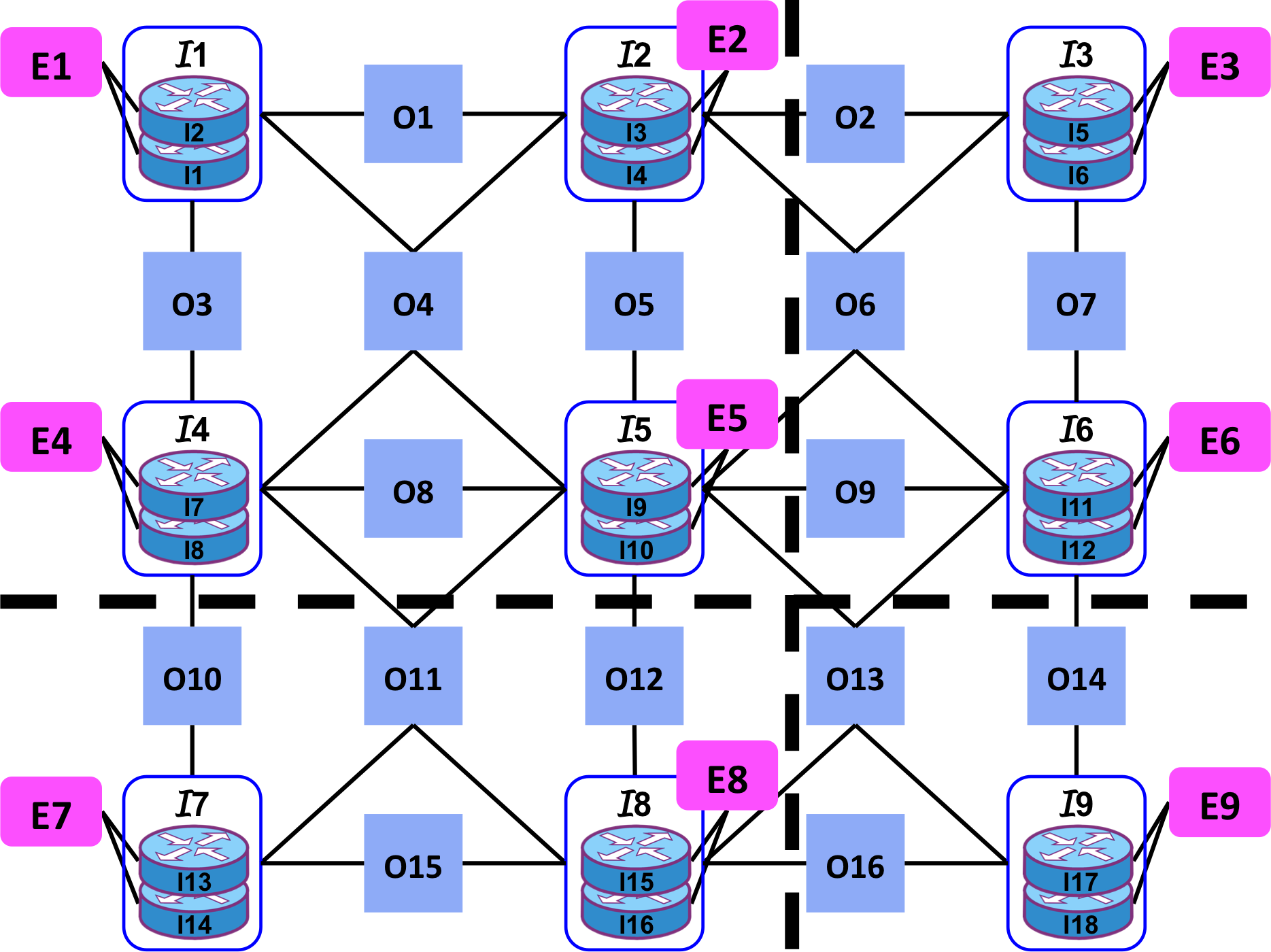
Figure 5: Topology used for experiments. We call the full network 9node-450/9node-600, the upper two-thirds (above the thick dashed line) 6node-450/6node-600, and the upper left corner 4node-450/4node-600.

For each topology, we use a traffic matrix in which each edge router sends 440 GB/sec to each other edge router. In our experiments we assume costs of 1 unit for each tail and 1 unit for each regen, while communication between colocated routers is free. We use Gurobi version 8 to solve our linear programs.

Alternative strategy. We compare Optimal, Greedy, and Simple to Legacy, the method currently used by ISPs to construct their networks. Once built, an IP link is fixed, and if any component fails, the link is down and all other components previously dedicated to it are unusable. In our Legacy algorithm, we assume that IP links follow the shortest optical path. Similar to Greedy, we begin by computing the optimal IP topology for the no failure case. We then designate those links as already paid for and solve the first failure case under the condition that reusing any of these links is “free.” We add any additional links placed in this iteration to the already-placed collection and repeat this process for all failure scenarios.

Legacy is the pure IP layer optimization and failure restoration described in Section II. As described previously, we need not compare our approaches to pure optical restoration, because pure optical restoration cannot recover from IP router failures. We need not compare against independent optical and IP restoration, because this technique generally performs worse than pure-IP or IP-along-disjoint-paths.

We compare against IP-along-shortest-paths, rather than IP-along-disjoint-paths, for two reasons. First, the main drawback of IP-along-shortest-paths is that, in general, it does not guarantee recovery from optical span failure. However, on our example topologies Legacy can handle any optical failure. Second, the formulation of the rigourous IP-along-djsoint-paths optimization is nearly as complex as the formulation of Optimal; if we remove the restriction that IP links must follow shortest paths, then we need constraints like those described in Section III-B to place regens every 1000 miles along a link’s path. For this reason, ISPs generally do not formulate and solve the rigorous IP-along-disjoint-paths optimization. Instead, they hand-place IP links according to heuristics and historical precedent. We don’t use this approach because it is too subjective and not scientifically replicable. In summary, IP-along-shortest-paths strikes the appropriate balance among (a) effectiveness at finding close to the optimal solution possible with traditional technology; (b) realism; (c) simplicity for our implementation and explanation; and (d) simplicity for the reader’s understanding and ability to replicate.

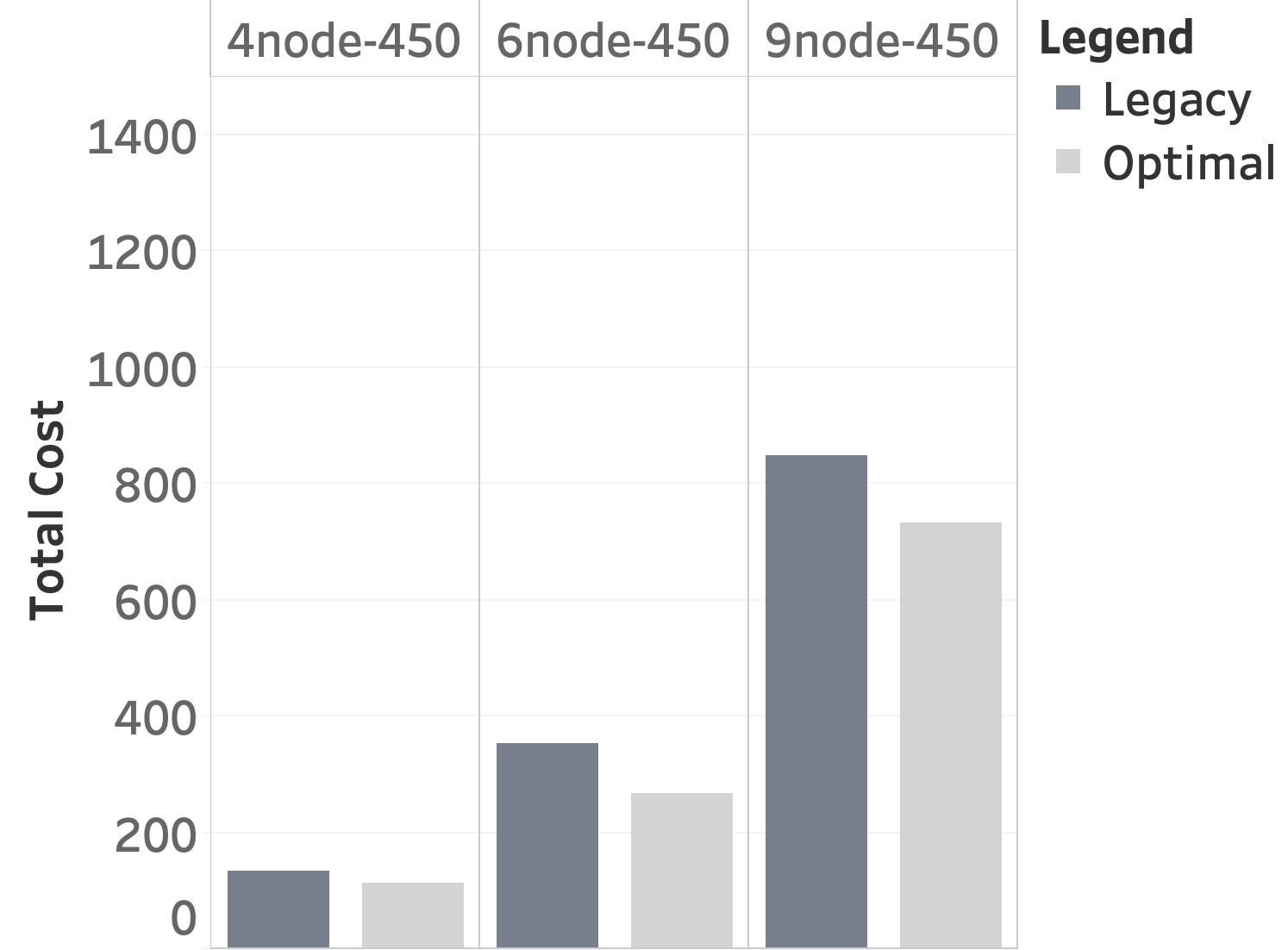
(a) Neighboring optical nodes 450 miles apart.

(b) Neighboring optical nodes 600 miles apart.

Figure 6: Total cost (tails + regens) by topology for Optimal and Legacy. Optimal outperforms Legacy on all topologies, and the gap is greatest on the largest network.

V-B Benefits of CD ROADMs

To justify the utility of CD ROADM technology, we show that building an optimal CD ROADM network offers up to 29% savings compared to building a legacy network. Since neither approach requires any regens on the 450 mile networks, all those savings come from tails. On 4node-600 Optimal requires 15% fewer tails and 38% fewer regens. On 6node-600 we achieve even greater savings, using 20% fewer tails and 44% fewer regens. On 9node-600 Optimal uses 16% more tails than Legacy but more than compensates by requiring 55% fewer regens, for an overall savings of 23%. The bars in Figures 6 illustrate the differences in total cost. Comparing Figures 6(a) and 6(b), we see that Optimal offers greater savings compared to Legacy on the 600 mile networks. This is because regens, moreso than tails, present opportunities for reuse across failure scenarios. Optimal capitalizes on this opportunity while Legacy doesn’t; both algorithms find solutions with close to the theoretical lower bound in tails, but Legacy in general is inefficient with regen placement. Since no regens are necessary for the 450 mile topologies, this benefit of Optimal compared to Legacy only manifests itself on the 600 mile networks.

In these experiments we allow up to five minutes per failure scenario for Legacy and the equivalent total time for Optimal (i.e., 300 sec $\times$ 21 failure scenarios = 6300 sec for 4node-450 and 4node-600, 300 sec $\times$ 35 failures = 10500 sec for 6node-450 and 6node-600 and $300\times 59=17700$ sec for 9node-450 and 9node-600).

V-C Scalability Benefits of Greedy

As Figure 7 shows, Greedy outperforms Optimal when both are limited to a short amount of time. “Short” here is relative to topology; Figure 7 illustrates that the crossover point is around 1200 seconds for 4node-600. In contrast, both Greedy and Optimal always outperform Simple, even at the shortest time limits. The design Greedy produces costs at most 1.3% more than the design generated by Optimal, while Simple’s design costs up to 12.4% more than that of Optimal and 11.0% more than that of Greedy. Reported times for these experiments do not parallelize Simple’s failure scenarios; we show the summed total time. In addition, the times for Greedy and Simple are an upper bound. We set a time limit of $t$ seconds for each of $|F|$ failure scenario, and we plot each algorithm’s objective value at $t|F|$.

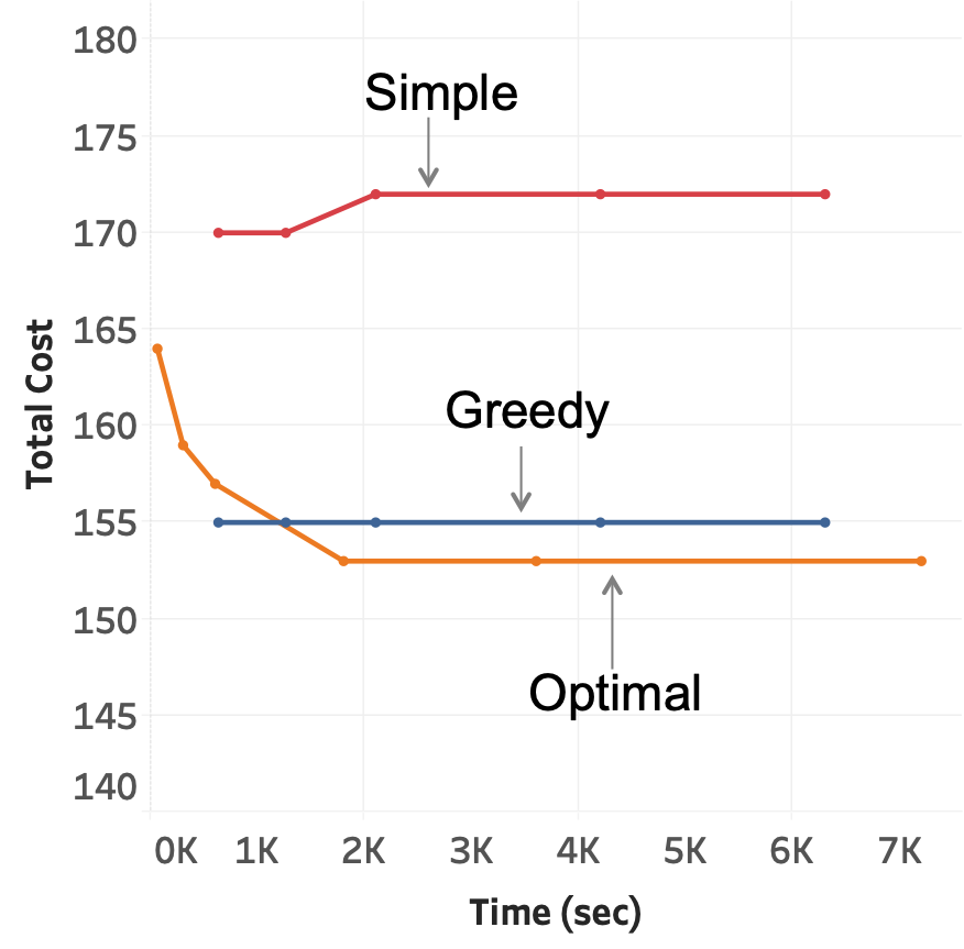
Figure 7: Total cost by computation time for Simple, Greedy, and Optimal on 4node-600. Lines do not start at $t=0$ because Gurobi requires some amount of time to find any feasible solution.

Interestingly, the objective values of Simple  for this topology, and Greedy for some others, do not monotonically decrease with increasing time. We suspect this is because their solutions for failure scenario $i$ depend on their solutions to all previous failures. Suppose that, on failure $i-j$, Gurobi finds a solution $s$ of cost $c$ after 60 seconds. If given 100 seconds per failure scenario, Gurobi might use the extra time to pivot from the particular solution $s$ to an equivalent cost solution $s^{\prime}$, in an endeavor to find a configuration with an objective value less than $c$ on this particular iteration. Since both $s$ and $s^{\prime}$ give a cost of $c$ for iteration $i-j$, Gurobi has no problem returning $s^{\prime}$. But, it’s possible that $s^{\prime}$ ultimately leads to a slightly worse overall solution than $s$. As Figure 7 shows, these differences are at most 10 tails and regens, and they occur only at the lowest time limits.

V-D Behavior During IP Link Reconfiguration

In the previous two subsections, we evaluate the steady-state performance of Optimal, along with Greedy, Simple, and Legacy, after the network has had time to transition both routing and the IP link configuration to their new optimal settings based on the current failure scenario. However, as we describe in Section II-C, there exists a period of approximately two minutes during which routing has already adapted to the new network conditions but IP links have not yet finished reconfiguration. In this section we show that our approach gracefully handles this transient period, as well.

The fundamental difference between these experiments and those in Sections V-B and V-C is that here we disallow IP link reconfiguration. Whereas in Sections V-B and V-C we jointly optimize both IP link configuration and routing in response to each failure scenario, we now reoptimize only routing; for each failure scenario we restrict ourselves to the links that were both already established in the no-failure case and have not been brought down by said failure. Specifically, in these experiments we begin with the no-failure IP link configuration as determined by Optimal. Then, one-by-one we consider each failure scenario, noting the fraction of offered traffic we can carry on this topology simply by switching from Optimal’s no-failure routing to whatever is now the best setup given the failure under consideration.

Figure 8 shows our results. The graphs are CDFs illustrating the fraction of failure scenarios indicated on the $y$-axis for which we can deliver at least the fraction of traffic denoted by the $x$-axis. For example, the red point at $(0.85,50\%)$ in Figure 8(a) indicates that in 50% of the 59 failure scenarios under consideration for 9node-450, we can deliver at least 85% of offered traffic just by reoptimizing routing. The blue line in Figure 8(a) represents the results of taking the 21 failure scenarios of 4node-450 in turn, and for each recording the fraction of offered traffic routed. The blue line in Figure 8(b) shows the same for the 21 failure scnarios of 4node-600, while the orange lines show the 35 failure scenarios for 6node-450 and 6node-600, and the red lines show the 59 failure scenarios for the large topologies.

We find two key takeaways from Figure 8. First, across all six topologies we always deliver at least 50% of traffic. Second, our results improve as the number of nodes in the network increases, and we do better on the topologies requiring regens than on those that don’t. On 9node-600, we’re always able to route at least 80% of traffic. Generally, ISPs’ SLAs require them to always deliver all high priority traffic, which typically represents about 40-60% of total load. However, in the presence of failures or extreme congestion they’re allowed to drop low priority traffic. Since most operational backbones are larger even than our 9node-600 topology, our results suggest that our algorithms should always allow ISPs to meet their SLAs. Note that we don’t expect to be able to route 100% of offered traffic in all failure scenarios without reconfiguring IP links; if we could there would be little reason to go through the reconfiguration process at all. But, we already saw in Section V-B that remapping the IP topology to the optical underlay adds significant value.

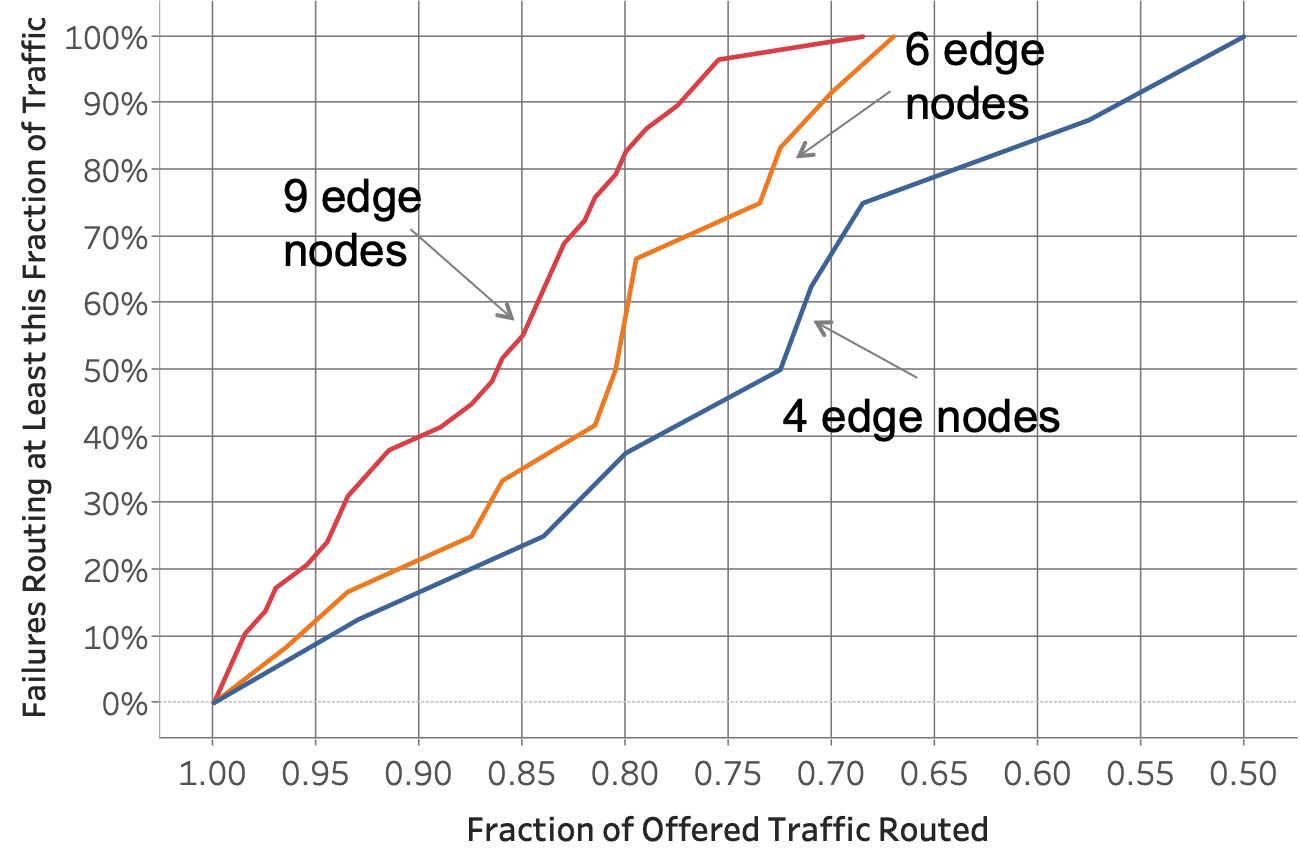
(a) Neighboring optical nodes 450 miles apart.

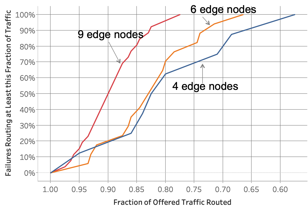
(b) Neighboring optical nodes 600 miles apart.

Figure 8: Percentage of failure scenarios for which rerouting over the existing IP links allows delivery of at least the indicated fraction of offered traffic.

VI Related Work

Though there has been significant work on various aspects of IP/optical networks, no existing research addresses the joint optimization of IP and optical network design.

At a high level, the Owan work by Jin et al. [8] is similar to ours. Like our work, Owan is a centralized system that jointly optimizes the IP and optical topologies and configures network devices, including CD ROADMs, according to this global strategy. However, there are three key differences between Owan and our work.

First, our objective differs from that of Jin et al. We aim to minimize the cost of tails and regens such that we place the equipment such that, under all failure scenarios, we can set up IP links to carry all necessary traffic. Jin et al. aim to minimize the transfer completion time or maximize the number of transfers that meet their deadlines.

Second, our work applies in a different setting. Owan is designed for bulk transfers and depends on the network operator being able to control sending rates, possibly delaying traffic for several hours. We target all ISP traffic; we can’t rate control any traffic, and we must route all demands, even in the case of failures, except during a brief transient period during IP link reconfiguration.

Third, we make different assumptions about what parts of the infrastructure are given and fixed. Jin et al. take the locations of optical equipment as an input constraint, while we solve for the optimal places to put tails and regens. This distinction is crucial; Jin et al. don’t need any notion of here-and-now decisions about where to place tails and regens separate from wait-and-see decisions about IP link configuration and routing.

Other studies demonstrate that, to minimize delay, it is best to set up direct IP links between endpoints exchanging significant amounts of traffic, while relying on packet switching through multiple hops to handle lower demands [9].

Choudhury [3] and Jin [8] consider joint IP/optical optimization but use heuristic algorithms.

VII Conclusion

Advances in optical technology and SDN have decoupled IP links from their underlying infrastructure (tails and regens). We have precisely stated and solved the new network design problem deriving from these advances, and we have also presented a fast approximation algorithm that comes very close to the optimal solution.

References

- [1] M. Birk, G. Choudhury, B. Cortez, A. Goddard, N. Padi, A. Raghuram, K. Tse, S. Tse, A. Wallace, and K. Xi, “Evolving to an SDN-enabled ISP backbone: Key technologies and applications,” IEEE Communications Magazine, vol. 54, no. 10, Oct. 2016.
- [2] G. Choudhury, M. Birk, B. Cortez, A. Goddard, N. Padi, K. Meier-Hellstern, J. Paggi, A. Raghuram, K. Tse, S. Tse, and A. Wallace, “Software defined networks to greatly improve the efficiency and flexibility of packet IP and optical networks,” in International Conference on Computing, Networking, and Communications, Jan. 2017.
- [3] G. Choudhury, D. Lynch, G. Thakur, and S. Tse, “Two use cases of machine learning for SDN-enabled IP/optical networks: Traffic matrix prediction and optical path performance prediction,” Journal of Optical Communications and Networking, vol. 10, no. 10, Oct. 2018.
- [4] S. Tse and G. Choudhury, “Real-time traffic management in AT&T’s SDN-enabled core IP/optical network,” in Optical Fiber Communication Conference and Exposition, Mar. 2018.
- [5] A. Chiu and J. Strand, “Joint IP/optical layer restoration after a router failure,” in Optical Fiber Communication Conference and Exposition, Mar. 2001.
- [6] A. Chiu, G. Choudhury, R. Doverspike, and G. Li, “Restoration design in IP over reconfigurable all-optical networks,” in IFIP International Conference on Network and Parallel Computing, ser. NPC, Sep. 2007.
- [7] A. L. Chiu, G. Choudhury, G. Clapp, R. Doverspike, M. Feuer, J. W. Gannett, J. Jackel, G. T. Kim, J. G. Klincewicz, T. J. Kwon, G. Li, P. Magill, J. M. Simmons, R. A. Skoog, J. Strand, A. V. Lehmen, B. J. Wilson, S. L. Woodward, and D. Xu, “Architectures and protocols for capacity efficient, highly dynamic and highly resilient core networks,” Journal of Optical Communications and Networking, vol. 4, no. 1, Jan. 2012.
- [8] X. Jin, Y. Li, D. Wei, S. Li, J. Gao, L. Xu, G. Li, W. Xu, and J. Rexford, “Optimizing bulk transfers with software-defined optical WAN,” in ACM SIGCOMM, Aug. 2016.
- [9] A. Brzezinski and E. Modiano, “Dynamic reconfiguration and routing algorithms for IP-over-WDM networks with stochastic traffic,” in IEEE INFOCOM 2005, Mar. 2005.