Regularity and convergence analysis in Sobolev and Hölder spaces for generalized Whittle–Matérn fields

Abstract.

We analyze several Galerkin approximations of a Gaussian random field $\mathcal{Z}\colon\mathcal{D}\times\Omega\to\mathbb{R}$ indexed by a Euclidean domain $\mathcal{D}\subset\mathbb{R}^{d}$ whose covariance structure is determined by a negative fractional power $L^{-2\beta}$ of a second-order elliptic differential operator $L:=-\nabla\cdot(A\nabla)+\kappa^{2}$. Under minimal assumptions on the domain $\mathcal{D}$, the coefficients $A\colon\mathcal{D}\to\mathbb{R}^{d\times d}$, $\kappa\colon\mathcal{D}\to\mathbb{R}$, and the fractional exponent $\beta>0$, we prove convergence in $L_{q}(\Omega;H^{\sigma}(\mathcal{D}))$ and in $L_{q}(\Omega;C^{\delta}(\overline{\mathcal{D}}))$ at (essentially) optimal rates for (i) spectral Galerkin methods and (ii) finite element approximations. Specifically, our analysis is solely based on $H^{1+\alpha}(\mathcal{D})$-regularity of the differential operator $L$, where $0<\alpha\leq 1$. For this setting, we furthermore provide rigorous estimates for the error in the covariance function of these approximations in $L_{\infty}(\mathcal{D}\times\mathcal{D})$ and in the mixed Sobolev space $H^{\sigma,\sigma}(\mathcal{D}\times\mathcal{D})$, showing convergence which is more than twice as fast compared to the corresponding $L_{q}(\Omega;H^{\sigma}(\mathcal{D}))$-rate.

For the well-known example of such Gaussian random fields, the original Whittle–Matérn class, where $L=-\Delta+\kappa^{2}$ and $\kappa\equiv\operatorname{const.}$, we perform several numerical experiments which validate our theoretical results.

1. Introduction

1.1. Motivation and background

By virtue of their practicality owing to the full characterization by their mean and covariance structure, Gaussian random fields (GRFs for short) are popular models for many applications in spatial statistics and uncertainty quantification, see, e.g., [4, 7, 26, 33, 35]. As a result, several methodologies in these disciplines require the efficient simulation of GRFs at unstructured locations in various possibly non-convex Euclidean domains, and this topic has been intensively discussed in both areas, spatial statistics and computational mathematics, see, e.g., [2, 8, 9, 13, 17, 19, 24, 30]. In particular, sampling from non-stationary GRFs, for which methods based on circulant embedding are inapplicable, has become a central topic of current research, see, e.g., [2, 9, 17].

In order to capture both stationary and non-stationary GRFs, a new class of random fields has been introduced in [26], which is based on the following observation made by P. Whittle [40]: A GRF $\mathcal{Z}$ on $\mathcal{D}:=\mathbb{R}^{d}$ with covariance function of Matérn type solves the fractional-order stochastic partial differential equation (SPDE for short)

$$L^{\beta}\mathcal{Z}=\mathrm{d}\mathcal{W},\quad\text{in }\mathcal{D},\qquad L:=-\Delta+\kappa^{2},$$ (1.1)

where $\Delta$ denotes the Laplacian, $\mathrm{d}\mathcal{W}$ is white noise on $\mathbb{R}^{d}$, and $\kappa>0$, $\beta>\nicefrac{{d}}{{4}}$ are constants which determine the practical correlation length and the smoothness of the field. In [26] this relation has been exploited to formulate generalizations of Matérn fields, the generalized Whittle–Matérn fields, by considering the SPDE (1.1) for non-stationary differential operators $L$ (e.g., by allowing for a spatially varying coefficient $\kappa\colon\mathcal{D}\to\mathbb{R}$) on bounded domains $\mathcal{D}\subset\mathbb{R}^{d}$, $d\in\{1,2,3\}$. Note that the covariance structure of a GRF is uniquely determined by its covariance operator, in this case given by the negative fractional-order differential operator $L^{-2\beta}$. Furthermore, for the case $2\beta\in\mathbb{N}$, approximations based on a finite element discretization have been proposed in [26].

Subsequently, a computational approach which allows for arbitrary fractional exponents $\beta>\nicefrac{{d}}{{4}}$ has been suggested in [2, 3]. To this end, a sinc quadrature combined with a Galerkin discretization of the differential operator $L$ is applied to the Balakrishnan integral representation of the fractional-order inverse $L^{-\beta}$.

In this work, we investigate Sobolev and Hölder regularity of generalized Whittle–Matérn fields and we perform a rigorous error analysis in these norms for several Galerkin approximations, including the sinc-Galerkin approximations of [2, 3]. Specifically, we consider a GRF $\mathcal{Z}^{\beta}\colon\mathcal{D}\times\Omega\to\mathbb{R}$, indexed by a Euclidean domain $\mathcal{D}\subset\mathbb{R}^{d}$, whose covariance operator is given by the negative fractional power $L^{-2\beta}$ of a second-order elliptic differential operator $L\colon\mathscr{D}(L)\subseteq L_{2}(\mathcal{D})\rightarrow L_{2}(\mathcal{D})$ in divergence form with Dirichlet boundary conditions, formally given by

$$Lu=-\nabla\cdot(A\nabla u)+\kappa^{2}u,\qquad u\in\mathscr{D}(L)\subseteq L_{2}(\mathcal{D}).$$ (1.2)

Here, we solely assume that $\mathcal{D}\subset\mathbb{R}^{d}$ has a Lipschitz boundary, $\kappa\in L_{\infty}(\mathcal{D})$, and that $A\in L_{\infty}\bigl{(}\mathcal{D};\mathbb{R}^{d\times d}\bigr{)}$ is symmetric and uniformly positive definite.

For a sequence $\bigl{(}\mathcal{Z}_{N}^{\beta}\bigr{)}_{N\in\mathbb{N}}$ of Galerkin approximations for $\mathcal{Z}^{\beta}$ (namely, spectral Galerkin approximations in Section 5 and sinc-Galerkin approximations in Section 6) defined with respect to family $(V_{N})_{N\in\mathbb{N}}$ of subspaces $V_{N}\subset H^{1}_{0}(\mathcal{D})$ of finite dimension $\dim(V_{N})=N<\infty$, we prove convergence at (essentially) optimal rates. More precisely, under minimal regularity conditions on the operator $L$ in (1.2) and for $0\leq\sigma<2\beta-\nicefrac{{d}}{{2}}$, $\delta\in(0,\sigma)$, within a suitable parameter range we show that for all $\varepsilon,q>0$ there exists a constant $C>0$ such that, for all $N\in\mathbb{N}$,

$$\left(\mathbb{E}\Bigl{[}\bigl{\|}\mathcal{Z}^{\beta}-\mathcal{Z}^{\beta}_{N}\bigr{\|}_{H^{\sigma}(\mathcal{D})}^{q}\Bigr{]}\right)^{\nicefrac{{1}}{{q}}} \leq CN^{-\nicefrac{{1}}{{d}}\,\left(2\beta-\sigma-\nicefrac{{d}}{{2}}-\varepsilon\right)},$$ (1.3)

$$\left(\mathbb{E}\Bigl{[}\bigl{\|}\mathcal{Z}^{\beta}-\mathcal{Z}^{\beta}_{N}\bigr{\|}_{C^{\delta}(\overline{\mathcal{D}})}^{q}\Bigr{]}\right)^{\nicefrac{{1}}{{q}}} \leq CN^{-\nicefrac{{1}}{{d}}\,\left(2\beta-\sigma-\nicefrac{{d}}{{2}}-\varepsilon\right)},$$ (1.4)

$$\bigl{\|}\varrho^{\beta}-\varrho^{\beta}_{N}\bigr{\|}_{H^{\sigma,\sigma}(\mathcal{D}\times\mathcal{D})} \leq CN^{-\nicefrac{{1}}{{d}}\,\left(4\beta-2\sigma-\nicefrac{{d}}{{2}}-\varepsilon\right)},$$ (1.5)

$$\sup_{x,y\in\overline{\mathcal{D}}}\bigl{|}\varrho^{\beta}(x,y)-\varrho^{\beta}_{N}(x,y)\bigr{|} \leq CN^{-\nicefrac{{1}}{{d}}\,\left(4\beta-d-\varepsilon\right)}.$$ (1.6)

Here, $\varrho^{\beta},\varrho_{N}^{\beta}\colon\mathcal{D}\times\mathcal{D}\to\mathbb{R}$ denote the covariance functions of the Whittle–Matérn field $\mathcal{Z}^{\beta}$ and of the Galerkin approximation $\mathcal{Z}_{N}^{\beta}$, respectively. For details, see Corollaries 5.1–5.3 for spectral Galerkin approximations, and Theorems 6.18, 6.23 for the sinc-Galerkin approach. “Suitable parameter range” refers to the observations that (i) if a finite element method of polynomial degree $p\in\mathbb{N}$ is used to define the sinc-Galerkin approximation or (ii) if $L$ in (1.2) is $H^{1+\alpha}(\mathcal{D})$-regular for $0<\alpha\leq 1$ maximal (see Definition 6.20), then the convergence rates of the sinc-Galerkin approximation cannot exceed $p+1-\sigma$ or $\min\{1+\alpha-\sigma,2\alpha\}$, where $0\leq\sigma\leq 1$.

We point out that due to the low regularity of white noise, $\mathrm{d}\mathcal{W}\in H^{-\nicefrac{{d}}{{2}}-\varepsilon}(\mathcal{D})$, which holds $\mathbb{P}$-almost surely and in $L_{q}(\Omega)$ (cf. [2, Prop. 2.3]) the convergence results (1.3)–(1.6) are (essentially, up to $\varepsilon>0$) optimal and they are also reflected in our numerical experiments, see Section 7 and the discussion in Section 8. Note furthermore that the convergence rates in (1.4), (1.6) of the field with respect to $L_{q}(\Omega;C^{\delta}(\overline{\mathcal{D}}))$ and of the covariance function in the $C(\overline{\mathcal{D}\times\mathcal{D}})$-norm, which we obtain via a Kolmogorov–Chentsov argument, are by $\nicefrac{{d}}{{2}}$ better than applying the results (1.3), (1.5) combined with the Sobolev embeddings $H^{\delta+\nicefrac{{d}}{{2}}}(\mathcal{D})\hookrightarrow C^{\delta}(\overline{\mathcal{D}})$ and $H^{\varepsilon+\nicefrac{{d}}{{2}},\,\varepsilon+\nicefrac{{d}}{{2}}}(\mathcal{D}\times\mathcal{D})\hookrightarrow C(\overline{\mathcal{D}\times\mathcal{D}})$, respectively. We remark that strong convergence of the sinc-Galerkin approximation with respect to the $L_{2}(\Omega;L_{2}(\mathcal{D}))$-norm, i.e., (1.3) for $\sigma=0$, at the rate $2\beta-\nicefrac{{d}}{{2}}$ has already been proven in [2, Thm. 2.10]. However, the assumptions made in [2, Ass. 2.6 and Eq. (2.19)] require the differential operator $L$ to be at least $H^{2}(\mathcal{D})$-regular. Thus, our results do not only generalize the analysis of [2] for the strong error to different norms, but also to less regular differential operators. This is of relevance for several practical applications, since the spatial domain, where the GRF is simulated, may be non-convex or the coefficient $A$ may have jumps. For this reason, in Subsection 6.3.2 we work under the assumption that $L$ is $H^{1+\alpha}(\mathcal{D})$-regular for some $0<\alpha\leq 1$ (for instance, $\alpha<\nicefrac{{\pi}}{{\omega}}$ if $\mathcal{D}$ is a non-convex domain with largest interior angle $\omega>\pi$).

As an interim result while deriving the error bounds (1.3)–(1.6) for the sinc-Galerkin approximation, we prove a non-trivial extension of one of the main results in [5]. Namely, we show that for all

$$\beta>0,\quad 0\leq\sigma\leq\min\{1,2\beta\},\quad-1\leq\delta\leq 1+\alpha,\ \delta\neq\nicefrac{{1}}{{2}}\quad\text{with}\quad 2\beta+\delta-\sigma>0,$$

and for all $\varepsilon>0$, there exists a constant $C>0$ such that, for $N\in\mathbb{N}$ and $g\in H^{\delta}(\mathcal{D})$,

$$\bigl{\|}L^{-\beta}g-\widetilde{L}_{N}^{-\beta}g\bigr{\|}_{H^{\sigma}(\mathcal{D})} \leq CN^{-\nicefrac{{1}}{{d}}\min\{2\beta+\delta-\sigma-\varepsilon,\,1+\alpha-\sigma,\,1+\alpha+\delta,\,2\alpha\}}\|g\|_{H^{\delta}(\mathcal{D})}.$$

Here, $\widetilde{L}_{N}^{-1}\colon H^{-1}(\mathcal{D})\to V_{N}$ denotes the approximation of the data-to-solution map $L^{-1}\colon H^{-1}(\mathcal{D})\to H^{1}_{0}(\mathcal{D})$ with respect to the Galerkin space $V_{N}\subset H^{1}_{0}(\mathcal{D})$. For details see Theorem 6.6, Remark 6.7 and Lemmata 6.21–6.22. This error estimate was proven in [5, Thm. 4.3 & Rem. 4.1] only for $\beta\in(0,1)$, $\sigma=0$, and $\delta\geq 0$, see also the comparison in Remark 6.8.

1.2. Outline

After specifying the mathematical setting as well as our notation in Subsections 1.3–1.4, we rigorously define the second-order elliptic differential operator $L$ from (1.2) under minimal assumptions on the coefficients $A,\kappa$ and the domain $\mathcal{D}\subset\mathbb{R}^{d}$ in Section 2; thereby collecting several auxiliary results for this type of operators. Section 3 is devoted to the regularity analysis of a GRF colored by a linear operator $T$ which is bounded on $L_{2}(\mathcal{D})$. These results are subsequently applied in Section 4 to the class of generalized Whittle–Matérn fields, where $T:=L^{-\beta}$ with $L$ defined as in Section 2 and $\beta>\nicefrac{{d}}{{4}}$. In Section 5 we derive the convergence results (1.3)–(1.6) for spectral Galerkin approximations where the finite-dimensional subspace $V_{N}$ is generated by the eigenvectors of the operator $L$ corresponding to the $N$ smallest eigenvalues. We then investigate sinc-Galerkin approximations in Section 6, where we first let $V_{N}$ be an abstract Galerkin space satisfying certain approximation properties, see Subsections 6.1–6.2. Subsequently, in Subsection 6.3 we show that these properties are indeed satisfied if the Galerkin spaces originate from a quasi-uniform family of finite element discretizations of polynomial degree $p\in\mathbb{N}$, and we discuss the convergence behavior for two cases in detail: (i) the coefficients $A,\kappa$ and the domain $\mathcal{D}$ in (1.2) are smooth, and (ii) $A,\kappa,\mathcal{D}$are such that the differential operator $L$ in (1.2) is only $H^{1+\alpha}(\mathcal{D})$-regular for some $0<\alpha\leq 1$. In Section 7 we perform several numerical experiments for the model example (1.1), $d=1$, and sinc-Galerkin discretizations generated with a finite element method of polynomial degree $p\in\{1,2\}$. In Section 8 we reflect on our outcomes.

1.3. Setting

Throughout this article, we let $(\Omega,\mathcal{F},\mathbb{P})$ be a complete probability space with expectation operator $\mathbb{E}$, and $\mathcal{D}$ be a bounded, connected and open subset of $\mathbb{R}^{d}$, $d\in\mathbb{N}$, with closure $\overline{\mathcal{D}}$.

In addition, we let $\mathcal{W}\colon L_{2}(\mathcal{D})\rightarrow L_{2}(\Omega)$ be an $L_{2}(\mathcal{D})$-isonormal Gaussian process in the sense of [29, Def. 1.1.1].

1.4. Notation

For $B\subseteq\mathbb{R}^{d}$, $\mathcal{B}(B)$ denotes the Borel $\sigma$-algebra on $B$ (i.e., the $\sigma$-algebra generated by the sets that are relatively open in $B$). For two $\sigma$-algebras $\mathcal{F}$ and $\mathcal{G}$, $\mathcal{F}\otimes\mathcal{G}$ is the $\sigma$-algebra generated by $\mathcal{F}\times\mathcal{G}$.

If $(E,\|\,\cdot\,\|_{E})$ is a Banach space, then $(E^{*},\|\,\cdot\,\|_{E^{*}})$ denotes its dual, $\langle\,\cdot\,,\,\cdot\,\rangle_{E^{*}\times E}$ the duality pairing on $E^{*}\times E$, $\operatorname{Id}_{E}$ the identity on $E$, and $\mathcal{L}(E;F)$ the space of bounded linear operators from $(E,\|\,\cdot\,\|_{E})$ to another Banach space $(F,\|\,\cdot\,\|_{F})$. For $T\in\mathcal{L}(E;F)$ we write $T^{*}\in\mathcal{L}(F^{*};E^{*})$ for the adjoint of $T$. If $V$ is a vector space such that $E,F\subseteq V$ and if, in addition, $\operatorname{Id}_{V}|_{E}\in\mathcal{L}(E;F)$, then we write $(E,\|\,\cdot\,\|_{E})\hookrightarrow(F,\|\,\cdot\,\|_{F})$. Moreover, the notation $(E,\|\,\cdot\,\|_{E})\cong(F,\|\,\cdot\,\|_{F})$ indicates that $(E,\|\,\cdot\,\|_{E})\hookrightarrow(F,\|\,\cdot\,\|_{F})\hookrightarrow(E,\|\,\cdot\,\|_{E})$.

If not specified otherwise, $(\,\cdot\,,\,\cdot\,)_{H}$ is the inner product on a Hilbert space $H$ and $\mathcal{L}_{2}(H;U)\subseteq\mathcal{L}(H;U)$ denotes the Hilbert space of Hilbert–Schmidt operators between two Hilbert spaces $H$ and $U$. The adjoint of $T\in\mathcal{L}(H;U)$ is identified with $T^{*}\in\mathcal{L}(U;H)$ (via the Riesz maps on $H$ and on $U$). We write $\mathcal{L}(E)$ and $\mathcal{L}_{2}(H)$ whenever $E=F$ and $H=U$. The domain of a possibly unbounded operator $L$ is denoted by $\mathscr{D}(L)$.

For $1\leq q<\infty$, $L_{q}(\mathcal{D};E)$ is the space of (equivalence classes of) $E$-valued, Bochner measurable, $q$-integrable functions on $\mathcal{D}$ and $L_{q}(\Omega;E)$ denotes the space of (equivalence classes of) $E$-valued random variables with finite $q$-th moment, i.e.,

$$\|f\|_{L_{q}(\mathcal{D};E)} :=\left(\int_{\mathcal{D}}\|f(x)\|_{E}^{q}\,\mathrm{d}x\right)^{\nicefrac{{1}}{{q}}}, f\in L_{q}(\mathcal{D};E),$$

$$\|X\|_{L_{q}(\Omega;E)} :=\left(\mathbb{E}\bigl{[}\|X\|_{E}^{q}\bigr{]}\right)^{\nicefrac{{1}}{{q}}}, X\in L_{q}(\Omega;E).$$

The space $L_{\infty}(\mathcal{D};E)$ consists of all equivalence classes of $E$-valued, Bochner measurable functions which are essentially bounded on $\mathcal{D}$, i.e.,

$$\|f\|_{L_{\infty}(\mathcal{D};E)}:=\operatorname{ess}\sup_{x\in\mathcal{D}}\|f(x)\|_{E},\qquad f\in L_{\infty}(\mathcal{D};E).$$

For $\gamma\in(0,1)$, we furthermore define the mappings

$$|\,\cdot\,|_{C^{\gamma}(\overline{\mathcal{D}};E)},\,\|\,\cdot\,\|_{C^{\gamma}(\overline{\mathcal{D}};E)}\colon C(\overline{\mathcal{D}};E)\to[0,\infty]$$

on the Banach space

$$\bigl{(}C(\overline{\mathcal{D}};E),\|\,\cdot\,\|_{C(\overline{\mathcal{D}};E)}\bigr{)},\qquad\|f\|_{C(\overline{\mathcal{D}};E)}:=\sup_{x\in\overline{\mathcal{D}}}\|f(x)\|_{E},$$

of continuous functions from $\overline{\mathcal{D}}$ to $(E,\|\,\cdot\,\|_{E})$ via

$$|f|_{C^{\gamma}(\overline{\mathcal{D}};E)} :=\sup_{\begin{subarray}{c}x,y\in\overline{\mathcal{D}}\\ x\neq y\end{subarray}}\frac{\|f(x)-f(y)\|_{E}}{|x-y|^{\gamma}},$$ (1.7)

$$\|f\|_{C^{\gamma}(\overline{\mathcal{D}};E)} :=\sup_{x\in\overline{\mathcal{D}}}\|f(x)\|_{E}+|f|_{C^{\gamma}(\overline{\mathcal{D}};E)}.$$ (1.8)

Note that the norm $\|\,\cdot\,\|_{C^{\gamma}(\overline{\mathcal{D}};E)}$ renders the subspace

$$C^{\gamma}(\overline{\mathcal{D}};E) =\left\{f\in C(\overline{\mathcal{D}};E):\|f\|_{C^{\gamma}(\overline{\mathcal{D}};E)}<\infty\right\}\subset C(\overline{\mathcal{D}};E)$$ (1.9)

of $\gamma$-Hölder continuous functions a Banach space. Whenever the functions or random variables are real-valued, we omit the image space and write $C(\overline{\mathcal{D}})$, $C^{\gamma}(\overline{\mathcal{D}})$, $L_{q}(\mathcal{D})$, and $L_{q}(\Omega)$, respectively. For $\sigma>0$, the (integer- or fractional-order) Sobolev space is denoted by $H^{\sigma}(\mathcal{D})$ (see [12, Sec. 2], see also [41, Sec. 1.11.4/5]), and $H^{1}_{0}(\mathcal{D})\subset H^{1}(\mathcal{D})$ is the closure of the space $C^{\infty}_{\operatorname{c}}(\mathcal{D})$ of compactly supported smooth functions in $\bigl{(}H^{1}(\mathcal{D}),\|\,\cdot\,\|_{H^{1}(\mathcal{D})}\bigr{)}$.

We mark equations which hold almost everywhere or $\mathbb{P}$-almost surely with a.e. and $\mathbb{P}$-a.s., respectively. For two random variables $X,Y$, we write $X\overset{d}{=}Y$ whenever $X$ and $Y$ have the same probability distribution. The Dirac measure at $x\in\overline{\mathcal{D}}$ is denoted by $\text{\dh}_{x}$. Given a parameter set $\mathcal{P}$ and mappings $A,B\colon\mathcal{P}\to\mathbb{R}$, we let $A(p)\lesssim B(p)$ denote the relation that there exists a constant $C>0$, independent of $p\in\mathcal{P}$, such that $A(p)\leq CB(p)$ for all $p\in\mathcal{P}$. For a further parameter set $\mathcal{Q}$ and mappings $A,B\colon\mathcal{P}\times\mathcal{Q}\rightarrow\mathbb{R}$, we write $A(p,q)\lesssim_{q}B(p,q)$ if, for all $q\in\mathcal{Q}$, there exists a constant $C_{q}>0$, independent of $p\in\mathcal{P}$, such that $A(p,q)\leq C_{q}B(p,q)$ for all $p\in\mathcal{P}$ and $q\in\mathcal{Q}$. Finally, $A(p)\eqsim B(p)$ indicates that both relations, $A(p)\lesssim B(p)$ and $B(p)\lesssim A(p)$, hold simultaneously; and similarly for $A(p,q)\eqsim_{q}B(p,q)$.

2. Auxiliary results on second-order elliptic differential operators

As outlined in Subsection 1.1, the overall objective of this article is to study (generalized) Whittle–Matérn fields and Galerkin approximations for them. Here, we call a Gaussian random field a generalized Whittle–Matérn field if its covariance operator is given by a negative fractional power of a second-order elliptic differential operator. The purpose of this section is to present preliminary results on second-order differential operators which will be of importance for the regularity and error analysis of these fields.

Firstly, we specify the class of differential operators that we consider. We start by formulating assumptions on the coefficients of the operator.

Assumption 2.1 (on the coefficients $A$ and $\kappa$).

Throughout this article we assume:

1. $A\in L_{\infty}\bigl{(}\mathcal{D};\mathbb{R}^{d\times d}\bigr{)}$ is symmetric and uniformly positive definite, i.e.,

   $$\exists a_{0}>0:\quad\operatorname{ess}\inf_{x\in\mathcal{D}}\xi^{\top}A(x)\xi\geq a_{0}|\xi|^{2}\quad\forall\xi\in\mathbb{R}^{d};$$ (2.1)

2. $\kappa\in L_{\infty}(\mathcal{D})$.

Where explicitly specified, we require in addition:

1. $A\colon\overline{\mathcal{D}}\to\mathbb{R}^{d\times d}$ is Lipschitz continuous on the closure $\overline{\mathcal{D}}$, i.e.,

   $$\exists a_{\operatorname{Lip}}>0:\quad|A_{ij}(x)-A_{ij}(y)|\leq a_{\operatorname{Lip}}|x-y|\quad\forall x,y\in\overline{\mathcal{D}},$$

   for all $i,j\in\{1,\ldots,d\}$.

Under Assumptions 2.1.I–II we let $L\colon\mathscr{D}(L)\subset L_{2}(\mathcal{D})\rightarrow L_{2}(\mathcal{D})$ denote the maximal accretive operator on $L_{2}(\mathcal{D})$ associated with $A$ and $\kappa^{2}$ with largest domain $\mathscr{D}(L)\subset H^{1}_{0}(\mathcal{D})$. By this we mean that $\mathscr{D}(L)$ consists of precisely those $u\in H^{1}_{0}(\mathcal{D})$ for which there exists a constant $C\geq 0$ such that

$$\left|\int_{\mathcal{D}}\bigl{[}(A(x)\nabla u(x),\nabla v(x))_{\mathbb{R}^{d}}+\kappa^{2}(x)u(x)v(x)\bigr{]}\,\mathrm{d}x\right|\leq C\|v\|_{L_{2}(\mathcal{D})}\quad\forall v\in H^{1}_{0}(\mathcal{D}),$$

and, for $u\in\mathscr{D}(L)$, $Lu$ is the unique element of $L_{2}(\mathcal{D})$ which, for all $v\in H^{1}_{0}(\mathcal{D})$, satisfies

$$\int_{\mathcal{D}}\bigl{[}(A(x)\nabla u(x),\nabla v(x))_{\mathbb{R}^{d}}+\kappa^{2}(x)u(x)v(x)\bigr{]}\,\mathrm{d}x=(Lu,v)_{L_{2}(\mathcal{D})}.$$ (2.2)

It is well-known that the operator $L\colon\mathscr{D}(L)\to L_{2}(\mathcal{D})$ defined via (2.2) is densely defined and self-adjoint (e.g., [31, Prop. 1.22 and Prop. 1.24]). Furthermore, by the Lax–Milgram lemma, its inverse exists and extends to a bounded linear operator $L^{-1}\colon H^{1}_{0}(\mathcal{D})^{*}\to H^{1}_{0}(\mathcal{D})$ (e.g., [31, Lem. 1.3]). By the Kondrachov compactness theorem $L^{-1}\colon L_{2}(\mathcal{D})\to L_{2}(\mathcal{D})$ is compact (e.g., [18, Thm. 7.22]).

For this reason, the spectrum of $L$ consists of a system of only positive eigenvalues $(\lambda_{j})_{j\in\mathbb{N}}$ with no accumulation point, whence we can assume them to be in nondecreasing order. The following asymptotic spectral behavior, known as Weyl’s law (see, e.g., [11, Thm. 6.3.1]), will be exploited several times in our analysis.

Lemma 2.2.

Let $L$ be the second-order differential operator in (2.2), defined with respect to the bounded open domain $\mathcal{D}\subset\mathbb{R}^{d}$, and with coefficients $A$ and $\kappa$ fulfilling Assumptions 2.1.I–II. Then, the eigenvalues of $L$ (in nondecreasing order) satisfy

$$\lambda_{j}\eqsim_{(A,\kappa,\mathcal{D})}j^{\nicefrac{{2}}{{d}}},\qquad j\in\mathbb{N}.$$ (2.3)

We let $\mathcal{E}:=\{e_{j}\}_{j\in\mathbb{N}}$ denote a system of eigenvectors of the operator $L$ in (2.2) which corresponds to the eigenvalues $(\lambda_{j})_{j\in\mathbb{N}}$ and which is orthonormal in $L_{2}(\mathcal{D})$. Note that, for $\sigma>0$, the fractional power operator $L^{\sigma}\colon\mathscr{D}(L^{\sigma})\subset L_{2}(\mathcal{D})\rightarrow L_{2}(\mathcal{D})$ is well-defined. Indeed, on the domain

$$\mathscr{D}(L^{\sigma}):=\Biggl{\{}\psi\in L_{2}(\mathcal{D}):\sum_{j\in\mathbb{N}}\lambda_{j}^{2\sigma}(\psi,e_{j})_{L_{2}(\mathcal{D})}^{2}<\infty\Biggr{\}}$$

the action of $L^{\sigma}$ is given via the spectral representation

$$L^{\sigma}\psi:=\sum_{j\in\mathbb{N}}\lambda_{j}^{\sigma}(\psi,e_{j})_{L_{2}(\mathcal{D})}e_{j},\qquad\psi\in\mathscr{D}(L^{\sigma}).$$

The subspace

$$\bigl{(}\dot{H}^{\sigma}_{L},(\,\cdot\,,\,\cdot\,)_{\sigma}\bigr{)},\qquad\dot{H}^{\sigma}_{L}:=\mathscr{D}\bigl{(}L^{\nicefrac{{\sigma}}{{2}}}\bigr{)}\subset L_{2}(\mathcal{D}),$$ (2.4)

is itself a Hilbert space with respect to the inner product

$$(\phi,\psi)_{\sigma}:=\bigl{(}L^{\nicefrac{{\sigma}}{{2}}}\phi,L^{\nicefrac{{\sigma}}{{2}}}\psi\bigr{)}_{L_{2}(\mathcal{D})}=\sum_{j\in\mathbb{N}}\lambda_{j}^{\sigma}(\phi,e_{j})_{L_{2}(\mathcal{D})}(\psi,e_{j})_{L_{2}(\mathcal{D})},$$

and the corresponding induced norm $\|\,\cdot\,\|_{\sigma}$. In what follows, we let $\dot{H}^{0}_{L}:=L_{2}(\mathcal{D})$ and, for $\sigma>0$, $\dot{H}^{-\sigma}_{L}$ denotes the dual space $(\dot{H}^{\sigma}_{L})^{*}$ after identification via the inner product $(\,\cdot\,,\,\cdot\,)_{L_{2}(\mathcal{D})}$ on $L_{2}(\mathcal{D})$ which is continuously extended to a duality pairing.

In order to derive regularity and convergence results with respect to the Sobolev space $H^{\sigma}(\mathcal{D})$ and the space $C^{\gamma}(\overline{\mathcal{D}})$ of $\gamma$-Hölder continuous functions in (1.9), we wish to relate the various norms involved by well-known results from interpolation theory and by Sobolev embeddings. To this end, we need to consider various assumptions on the spatial domain $\mathcal{D}$, specified below.

Assumption 2.3 (on the domain $\mathcal{D}$).

Throughout this article, we assume that

1. $\mathcal{D}$ has a Lipschitz continuous boundary $\partial\mathcal{D}$.

Where explicitly specified, we additionally suppose one or both of the following:

1. $\mathcal{D}$ is convex;

2. $\mathcal{D}$ is a polytope.

Note that II. implies I. (see, e.g., [21, Cor. 1.2.2.3]).

In the following lemma we specify the relationship between the spaces $\dot{H}^{\sigma}_{L}$ in (2.4) and the Sobolev space $H^{\sigma}(\mathcal{D})$, under two sets of assumptions on the spatial domain $\mathcal{D}$ and on the coefficients $A$, $\kappa$ of the differential operator $L$ in (2.2). We recall that $[E,F]_{\sigma}$ denotes the complex interpolation space between $(E,\|\,\cdot\,\|_{E})$ and $(F,\|\,\cdot\,\|_{F})$ with parameter $\sigma\in[0,1]$, see, e.g., [27, Ch. 2].

Lemma 2.4.

Let Assumptions 2.1.I–II and 2.3.I be satisfied. Then

$$\bigl{(}\dot{H}^{\sigma}_{L},\|\,\cdot\,\|_{\sigma}\bigr{)}\cong\bigl{(}\left[L_{2}(\mathcal{D}),H^{1}_{0}(\mathcal{D})\right]_{\sigma},\|\,\cdot\,\|_{[L_{2}(\mathcal{D}),H^{1}_{0}(\mathcal{D})]_{\sigma}}\bigr{)},\qquad 0\leq\sigma\leq 1,$$ (2.5)

holds for the space $\bigl{(}\dot{H}^{\sigma}_{L},\|\,\cdot\,\|_{\sigma}\bigr{)}$ from (2.4). Furthermore,

$$\bigl{(}\dot{H}^{\sigma}_{L},\|\,\cdot\,\|_{\sigma}\bigr{)}\hookrightarrow\bigl{(}H^{\sigma}(\mathcal{D}),\|\,\cdot\,\|_{H^{\sigma}(\mathcal{D})}\bigr{)},\qquad 0\leq\sigma\leq 1,$$ (2.6)

and the norms $\|\,\cdot\,\|_{\sigma}$, $\|\,\cdot\,\|_{H^{\sigma}(\mathcal{D})}$ are equivalent on $\dot{H}^{\sigma}_{L}$ for $0\leq\sigma\leq 1$ and $\sigma\neq\nicefrac{{1}}{{2}}$. If, in addition, Assumptions 2.1.III and 2.3.II hold, then

$$\bigl{(}\dot{H}^{\sigma}_{L},\|\,\cdot\,\|_{\sigma}\bigr{)}\cong\bigl{(}H^{\sigma}(\mathcal{D})\cap H^{1}_{0}(\mathcal{D}),\|\,\cdot\,\|_{H^{\sigma}(\mathcal{D})}\bigr{)},\qquad 1\leq\sigma\leq 2.$$ (2.7)

Proof.

First, note that [41, Cor. 2.4] implies (2.5). If $(E,\|\,\cdot\,\|_{E})$, $(F,\|\,\cdot\,\|_{F})$, and $(G,\|\,\cdot\,\|_{G})$ are Banach spaces such that $(F,\|\,\cdot\,\|_{F})\hookrightarrow(G,\|\,\cdot\,\|_{G})$, then by definition of complex interpolation we have $\bigl{(}[E,F]_{\sigma},\|\,\cdot\,\|_{[E,F]_{\sigma}}\bigr{)}\hookrightarrow\bigl{(}[E,G]_{\sigma},\|\,\cdot\,\|_{[E,G]_{\sigma}}\bigr{)}$. This observation in connection with [41, Thm. 1.35] (which collects several results from [39]) shows (2.6). Equivalence of $\|\,\cdot\,\|_{\sigma}$, $\|\,\cdot\,\|_{H^{\sigma}(\mathcal{D})}$ on $\dot{H}^{\sigma}_{L}$ for $0\leq\sigma\leq 1$, $\sigma\neq\nicefrac{{1}}{{2}}$, is proven in [20, Thm. 8.1]. By combining (2.5) for $\sigma=1$, [27, Thm. 4.36] and [22, Lem. A2] (recalling Assumption 2.3.II) we find that (2.7) for $\sigma\in(1,2)$ follows once (2.7) is established for the case $\sigma=2$.

It thus remains to prove (2.7) for $\sigma=2$. To this end, we first observe that, for a vanishing coefficient $\kappa\equiv 0$ of the operator $L$ in (2.2), we have, e.g., by [21, Thm. 3.2.1.2] the regularity result

$$f\in L_{2}(\mathcal{D})\quad\Rightarrow\quad u:=L^{-1}f\in H^{2}(\mathcal{D})\cap H^{1}_{0}(\mathcal{D}).$$ (2.8)

If $\kappa\not\equiv 0$, then $u\in H^{1}_{0}(\mathcal{D})$ satisfies the equality $-\nabla\cdot(A\nabla u)=f-\kappa^{2}u$ in the weak sense so that [21, Thm. 3.2.1.2] applied to $\widetilde{f}:=f-\kappa^{2}u\in L_{2}(\mathcal{D})$ again yields (2.8). By the closed graph theorem, $\bigl{(}\dot{H}^{2}_{L},\|\,\cdot\,\|_{2}\bigr{)}\hookrightarrow\bigl{(}H^{2}(\mathcal{D})\cap H^{1}_{0}(\mathcal{D}),\|\,\cdot\,\|_{H^{2}(\mathcal{D})}\bigr{)}$.

We now establish the reverse embedding. By Assumption 2.1.III and, e.g., [16, Thm. 4 in Ch. 5.8] (note that the assumptions on the boundary posed therein can be circumvented by exploiting an extension argument as, e.g., in [36, Sec. VI.2.3 Thm. 3], see also the remark below [16, Thm. 4 in Ch. 5.8]), $A_{ij}$ is differentiable a.e. in $\mathcal{D}$ with essentially bounded weak derivatives $\partial_{x_{k}}A_{ij}\in L_{\infty}(\mathcal{D})$, $1\leq i,j,k\leq d$. Thus (by first approximating $A_{ij}$ in $H^{1}(\mathcal{D})$ with a sequence in $C^{\infty}(\mathcal{D})$ to obtain that $A_{ij}\partial_{x_{j}}u$ is weakly differentiable with $\partial_{x_{k}}(A_{ij}\partial_{x_{j}}u)=\partial_{x_{k}}A_{ij}\partial_{x_{j}}u+A\partial_{x_{k}x_{j}}u$), we conclude that $A\nabla u\in H^{1}(\mathcal{D})^{d}$ whenever $u\in H^{2}(\mathcal{D})\cap H^{1}_{0}(\mathcal{D})$. Finally, by the closed graph theorem $\bigl{(}H^{2}(\mathcal{D})\cap H^{1}_{0}(\mathcal{D}),\|\,\cdot\,\|_{H^{2}(\mathcal{D})}\bigr{)}\hookrightarrow\bigl{(}\dot{H}^{2}_{L},\|\,\cdot\,\|_{2}\bigr{)}$ follows. ∎

3. General results on Gaussian Random Fields (GRFs)

In this section we address different notions of regularity (Hölder and Sobolev) for Gaussian random fields (GRFs) and their covariance functions. We first recall the definition of a GRF and specify then what we mean by a colored GRF. As usually, we work in the setting formulated in Subsection 1.3.

Definition 3.1.

Let $B\subseteq\mathbb{R}^{d}$. A family of $\mathcal{F}$-measurable $\mathbb{R}$-valued random variables $(\mathcal{Z}(x))_{x\in B}$ is called a random field (indexed by $B$). It is called Gaussian if the random vector $(\mathcal{Z}(x_{1}),\ldots,\mathcal{Z}(x_{n}))^{\top}$ is Gaussian for all finite sets $\{x_{1},\ldots,x_{n}\}\subset B$. It is called continuous if the mapping $x\mapsto\mathcal{Z}(x)(\omega)$ is continuous for all $\omega\in\Omega$.

Definition 3.2.

Let $T\in\mathcal{L}(L_{2}(\mathcal{D}))$. We call $\mathcal{Z}\colon\mathcal{D}\times\Omega\rightarrow\mathbb{R}$ a Gaussian random field (GRF) colored by $T$ if it is a GRF, a $\mathcal{B}(\mathcal{D})\otimes\mathcal{F}$-measurable mapping, and

$$(\mathcal{Z},\psi)_{L_{2}(\mathcal{D})}=\mathcal{W}(T^{*}\psi)\quad\mathbb{P}\text{-a.s.}\quad\forall\psi\in L_{2}(\mathcal{D}).$$ (3.1)

Remark 3.3.

It is well-known and easily verified (see also Proposition 3.7) that there exists a square-integrable GRF $\mathcal{Z}$ colored by $T$ if and only if $T\in\mathcal{L}_{2}(L_{2}(\mathcal{D}))$, and in this case $\mathbb{E}\bigl{[}\|\mathcal{Z}\|_{L_{2}(\mathcal{D})}^{2}\bigr{]}=\operatorname{tr}(TT^{*})$, where $\operatorname{tr}(\,\cdot\,)$ is the trace on $L_{2}(\mathcal{D})$.

3.1. Hölder regularity of GRFs

We now provide an abstract result on the construction and Hölder regularity of a GRF assuming that the color and, thus, the covariance structure of the field is given.

Proposition 3.4.

Assume that $T\in\mathcal{L}(L_{2}(\mathcal{D});C^{\gamma}(\overline{\mathcal{D}}))$ for some $\gamma\in(0,1)$. Then there exists a continuous GRF $\mathcal{Z}$ colored by $T$ such that

$$\mathcal{Z}(x)=\mathcal{W}(T^{*}\text{\dh}_{x})\quad\mathbb{P}\text{-a.s.}\quad\forall x\in\overline{\mathcal{D}}.$$ (3.2)

Furthermore, for $q\in(0,\infty)$ and $\delta\in(0,\gamma)$, we have

$$\left(\mathbb{E}\Bigl{[}\|\mathcal{Z}\|_{C^{\delta}(\overline{\mathcal{D}})}^{q}\Bigr{]}\right)^{\nicefrac{{1}}{{q}}}\lesssim_{(q,\gamma,\delta,\mathcal{D})}\|T\|_{\mathcal{L}(L_{2}(\mathcal{D});C^{\gamma}(\overline{\mathcal{D}}))}.$$ (3.3)

Proof.

We first define the random field $\mathcal{Z}_{0}\colon\overline{\mathcal{D}}\times\Omega\to\mathbb{R}$ by $\mathcal{Z}_{0}(x):=\mathcal{W}(T^{*}\text{\dh}_{x})$ for all $x\in\overline{\mathcal{D}}$. By the properties of an isonormal Gaussian process we find, for $x,y\in\overline{\mathcal{D}}$,

$$\left(\mathbb{E}\bigl{[}|\mathcal{Z}_{0}(x)-\mathcal{Z}_{0}(y)|^{2}\bigr{]}\right)^{\nicefrac{{1}}{{2}}} =\left(\mathbb{E}\bigl{[}|\mathcal{W}(T^{*}(\text{\dh}_{x}-\text{\dh}_{y}))|^{2}\bigr{]}\right)^{\nicefrac{{1}}{{2}}}=\|T^{*}(\text{\dh}_{x}-\text{\dh}_{y})\|_{L_{2}(\mathcal{D})^{*}}$$

$$\leq\|T^{*}\|_{\mathcal{L}(C^{\gamma}(\overline{\mathcal{D}})^{*};L_{2}(\mathcal{D})^{*})}\|\text{\dh}_{x}-\text{\dh}_{y}\|_{C^{\gamma}(\overline{\mathcal{D}})^{*}}$$

$$=\|T\|_{\mathcal{L}(L_{2}(\mathcal{D});C^{\gamma}(\overline{\mathcal{D}}))}|x-y|^{\gamma}.$$ (3.4)

Since $\mathcal{Z}_{0}(x)-\mathcal{Z}_{0}(y)=\mathcal{W}(T^{*}(\text{\dh}_{x}-\text{\dh}_{y}))$ is a real-valued Gaussian random variable, we can apply the Khintchine inequalities (see, e.g., [25, Thm. 4.7 and p. 103]) and conclude with (3.4) that, for all $q\in(0,\infty)$, the estimate

$$|\mathcal{Z}_{0}|_{C^{\gamma}(\overline{\mathcal{D}};L_{q}(\Omega))} \leq C_{q}\sup\limits_{\begin{subarray}{c}x,y\in\overline{\mathcal{D}}\\ x\neq y\end{subarray}}\left(\mathbb{E}\Biggl{[}\left|\frac{\mathcal{Z}_{0}(x)-\mathcal{Z}_{0}(y)}{|x-y|^{\gamma}}\right|^{2}\Biggr{]}\right)^{\nicefrac{{1}}{{2}}}$$

$$\leq C_{q}\|T\|_{\mathcal{L}(L_{2}(\mathcal{D});C^{\gamma}(\overline{\mathcal{D}}))}$$ (3.5)

holds, with a constant $C_{q}>0$ depending only on $q$.

Thus, by the Kolmogorov–Chentsov continuity theorem (e.g., [34, Thm. I.2.1], combined with an extension argument as discussed in the proof of [28, Thm. 2.1], see also [36, Thm. VI.2.3]), there exists a continuous random field $\mathcal{Z}\colon\overline{\mathcal{D}}\times\Omega\to\mathbb{R}$ such that $\mathcal{Z}(x)=\mathcal{Z}_{0}(x)$ $\mathbb{P}$-a.s. for all $x\in\overline{\mathcal{D}}$, and furthermore, for every $\delta\in(0,\gamma)$ and every finite $q>(\gamma-\delta)^{-1}$, we can find a constant $C_{q,\gamma,\delta,\mathcal{D}}>0$, depending only on $q$, $\gamma$, $\delta$, as well as the dimension and the diameter of $\mathcal{D}\subset\mathbb{R}^{d}$, such that

$$\left(\mathbb{E}\Bigl{[}|\mathcal{Z}|_{C^{\delta}(\overline{\mathcal{D}})}^{q}\Bigr{]}\right)^{\nicefrac{{1}}{{q}}}\leq C_{q,\gamma,\delta,\mathcal{D}}|\mathcal{Z}_{0}|_{C^{\gamma}(\overline{\mathcal{D}};L_{q}(\Omega))}.$$ (3.6)

Next, again by the Khintchine inequalities, we have, for all $x\in\overline{\mathcal{D}}$ and all $q\in(0,\infty)$,

$$\left(\mathbb{E}\left[|\mathcal{Z}(x)|^{q}\right]\right)^{\nicefrac{{1}}{{q}}} =\left(\mathbb{E}\left[|\mathcal{Z}_{0}(x)|^{q}\right]\right)^{\nicefrac{{1}}{{q}}}$$

$$\leq C_{q}\left(\mathbb{E}\left[|\mathcal{W}(T^{*}\text{\dh}_{x})|^{2}\right]\right)^{\nicefrac{{1}}{{2}}}\leq C_{q}\|T\|_{\mathcal{L}(L_{2}(\mathcal{D});C^{\gamma}(\overline{\mathcal{D}}))}.$$ (3.7)

From (1.7)–(1.8) we deduce, for every $\delta\in(0,1)$ and all $f\in C^{\delta}(\overline{\mathcal{D}})$, the relation

$$\|f\|_{C^{\delta}(\overline{\mathcal{D}})}\leq|f(x)|+\bigl{(}1+\operatorname{diam}(\mathcal{D})^{\delta}\bigr{)}|f|_{C^{\delta}(\overline{\mathcal{D}})}\quad\forall x\in\overline{\mathcal{D}}.$$

We combine this observation with (3.5), (3.6), and (3.7) to derive, for all $\delta\in(0,\gamma)$ and all finite $q>(\gamma-\delta)^{-1}$, the bound

$$\left(\mathbb{E}\Bigl{[}\|\mathcal{Z}\|_{C^{\delta}(\overline{\mathcal{D}})}^{q}\Bigr{]}\right)^{\nicefrac{{1}}{{q}}} \leq C_{q}\|T\|_{\mathcal{L}(L_{2}(\mathcal{D});C^{\gamma}(\overline{\mathcal{D}}))}+\bigl{(}1+\operatorname{diam}(\mathcal{D})^{\delta}\bigr{)}\left(\mathbb{E}\Bigl{[}|\mathcal{Z}|_{C^{\delta}(\overline{\mathcal{D}})}^{q}\Bigr{]}\right)^{\nicefrac{{1}}{{q}}}$$

$$\leq C_{q}\bigl{(}1+C_{q,\gamma,\delta,\mathcal{D}}\bigl{(}1+\operatorname{diam}(\mathcal{D})^{\delta}\bigr{)}\bigr{)}\|T\|_{\mathcal{L}(L_{2}(\mathcal{D});C^{\gamma}(\overline{\mathcal{D}}))}.$$ (3.8)

Note that Hölder’s inequality and (3.8) ensure that (3.3) holds for every $\delta\in(0,\gamma)$ and every $q\in(0,\infty)$. Furthermore, for every $\psi\in L_{2}(\mathcal{D})$, one readily verifies the identity $\mathbb{E}\bigl{[}|(\mathcal{Z},\psi)_{L_{2}(\mathcal{D})}-\mathcal{W}(T^{*}\psi)|^{2}\bigr{]}=0$, i.e., $\mathcal{Z}$ is colored by $T$. ∎

If Assumption 2.3.I is fulfilled, the Sobolev embedding theorem (see, e.g., [12, Thm. 5.4 and Thm. 8.2]) is applicable and we obtain $\gamma$-Hölder continuity (1.9) for elements in the fractional-order Sobolev space $H^{\gamma+\nicefrac{{d}}{{2}}}(\mathcal{D})$ for every $\gamma\in(0,1)$. This continuous embedding, $H^{\gamma+\nicefrac{{d}}{{2}}}(\mathcal{D})\hookrightarrow C^{\gamma}(\overline{\mathcal{D}})$, combined with Proposition 3.4 leads to the following result.

Corollary 3.5.

Let Assumption 2.3.I, $\gamma\in(0,1)$, and $T\in\mathcal{L}\bigl{(}L_{2}(\mathcal{D});H^{\gamma+\nicefrac{{d}}{{2}}}(\mathcal{D})\bigr{)}$ be satisfied. Then there exists a continuous GRF $\mathcal{Z}\colon\overline{\mathcal{D}}\times\Omega\rightarrow\mathbb{R}$ colored by $T$, cf. (3.1), such that $\mathcal{Z}(x)=\mathcal{W}(T^{*}\text{\dh}_{x})$ $\mathbb{P}$-a.s. for all $x\in\overline{\mathcal{D}}$. Moreover, the stability estimate

$$\left(\mathbb{E}\Bigl{[}\|\mathcal{Z}\|_{C^{\delta}(\overline{\mathcal{D}})}^{q}\Bigr{]}\right)^{\nicefrac{{1}}{{q}}}\lesssim_{(q,\gamma,\delta,\mathcal{D})}\|T\|_{\mathcal{L}\left(L_{2}(\mathcal{D});H^{\gamma+\nicefrac{{d}}{{2}}}(\mathcal{D})\right)}$$ (3.9)

for the $q$-th moment of $\mathcal{Z}$ with respect to the $\delta$-Hölder norm (1.8) holds for every $\delta\in(0,\gamma)$ and $q\in(0,\infty)$.

We close the subsection with a brief discussion on (i) the continuity of covariance functions of colored GRFs, and (ii) the $L_{\infty}(\mathcal{D}\times\mathcal{D})$-distance between two covariance functions of GRFs colored by different operators.

By definition, the covariance function $\varrho\in L_{2}(\mathcal{D}\times\mathcal{D})$ of a square-integrable random field $\mathcal{Z}\in L_{2}(\mathcal{D}\times\Omega)$ satisfies

$$\varrho(x,y)=\mathbb{E}[(\mathcal{Z}(x)-\mathbb{E}[\mathcal{Z}(x)])(\mathcal{Z}(y)-\mathbb{E}[\mathcal{Z}(y)])]\quad\text{a.e.\ in }\mathcal{D}\times\mathcal{D}.$$ (3.10)

We obtain the one-to-one correspondence

$$\int_{\mathcal{D}}\varrho(x,y)\psi(y)\,\mathrm{d}y=(\mathcal{C}\psi)(x)\quad\text{a.e.\ in }\mathcal{D},\quad\forall\psi\in L_{2}(\mathcal{D}),$$

with the covariance operator $\mathcal{C}\colon L_{2}(\mathcal{D})\to L_{2}(\mathcal{D})$ of the field $\mathcal{Z}$, which is defined via

$$(\mathcal{C}\phi,\psi)_{L_{2}(\mathcal{D})}=\mathbb{E}\bigl{[}(\mathcal{Z}-\mathbb{E}[\mathcal{Z}],\phi)_{L_{2}(\mathcal{D})}(\mathcal{Z}-\mathbb{E}[\mathcal{Z}],\psi)_{L_{2}(\mathcal{D})}\bigr{]}\quad\forall\phi,\psi\in L_{2}(\mathcal{D}).$$

From this definition it is evident that a GRF $\mathcal{Z}$ colored by $T$ (note that $\mathbb{E}[\mathcal{Z}]=0$ by construction, see Definition 3.2) has the covariance operator $\mathcal{C}=TT^{*}$. In the next lemma, this relation is exploited to characterize continuity of the covariance function $\varrho$ in terms of the color $T$ of the GRF $\mathcal{Z}$.

Proposition 3.6.

Let $\mathcal{Z},\widetilde{\mathcal{Z}}$ be GRFs colored by $T$ and $\widetilde{T}$, respectively, see (3.1), with covariance functions denoted by $\varrho$ and $\widetilde{\varrho}$, cf. (3.10). Then,

1. $\varrho$ has a continuous representative on $\overline{\mathcal{D}\times\mathcal{D}}$ (again denoted by $\varrho$) if and only if $T\in\mathcal{L}(L_{2}(\mathcal{D});C(\overline{\mathcal{D}}))$. In this case,

   $$\sup_{x,y\in\overline{\mathcal{D}}}|\varrho(x,y)|\leq\|TT^{*}\|_{\mathcal{L}(C(\overline{\mathcal{D}})^{*};C(\overline{\mathcal{D}}))}\,;$$ (3.11)

2. if $T,\widetilde{T}\in\mathcal{L}(L_{2}(\mathcal{D});C(\overline{\mathcal{D}}))$, then $\varrho,\widetilde{\varrho}\in C(\overline{\mathcal{D}\times\mathcal{D}})$ satisfy

   $$\sup_{x,y\in\overline{\mathcal{D}}}\bigl{|}\varrho(x,y)-\widetilde{\varrho}(x,y)\bigr{|}\leq\bigl{\|}TT^{*}-\widetilde{T}\widetilde{T}^{*}\bigr{\|}_{\mathcal{L}(C(\overline{\mathcal{D}})^{*};C(\overline{\mathcal{D}}))}\,.$$ (3.12)

Proof.

By (3.10), the covariance function $\varrho$ of a GRF $\mathcal{Z}$ colored by $T$ is given by

$$\varrho(x,y)=(T^{*}\text{\dh}_{x},T^{*}\text{\dh}_{y})_{L_{2}(\mathcal{D})^{*}}\quad\text{a.e.\ in }\overline{\mathcal{D}\times\mathcal{D}}.$$ (3.13)

First, let $T\in\mathcal{L}(L_{2}(\mathcal{D});C(\overline{\mathcal{D}}))$. Then, we have $T^{*}\in\mathcal{L}(C(\overline{\mathcal{D}})^{*};L_{2}(\mathcal{D})^{*})$ and continuity of $\varrho\colon\overline{\mathcal{D}\times\mathcal{D}}\to\mathbb{R}$ follows from (3.13). Assume now that $\varrho\in C(\overline{\mathcal{D}\times\mathcal{D}})$. Then, again by (3.13), we obtain $\|T^{*}\text{\dh}_{x}\|_{L_{2}(\mathcal{D})^{*}}^{2}=\varrho(x,x)<\infty$ for all $x\in\overline{\mathcal{D}}$ and

$$\|T\phi\|_{C(\overline{\mathcal{D}})}=\sup_{x\in\overline{\mathcal{D}}}\langle\text{\dh}_{x},T\phi\rangle_{C(\overline{\mathcal{D}})^{*}\times C(\overline{\mathcal{D}})}\leq\sup_{x\in\overline{\mathcal{D}}}\|T^{*}\text{\dh}_{x}\|_{L_{2}(\mathcal{D})^{*}}<\infty$$

holds for all $\phi\in L_{2}(\mathcal{D})$ with $\|\phi\|_{L_{2}(\mathcal{D})}\leq 1$. Thus, $T\in\mathcal{L}(L_{2}(\mathcal{D});C(\overline{\mathcal{D}}))$ if $\varrho$ is continuous. Furthermore, by identifying $L_{2}(\mathcal{D})^{*}\cong L_{2}(\mathcal{D})$ via the Riesz map, the covariance operator $\mathcal{C}$ of $\mathcal{Z}$ satisfies $\mathcal{C}=TT^{*}\in\mathcal{L}(C(\overline{\mathcal{D}})^{*};C(\overline{\mathcal{D}}))$, and we can deduce (3.11) from (3.13) since, for all $x,y\in\overline{\mathcal{D}}$,

$$|\varrho(x,y)|=|\langle\text{\dh}_{x},TT^{*}\text{\dh}_{y}\rangle_{C(\overline{\mathcal{D}})^{*}\times C(\overline{\mathcal{D}})}|\leq\|TT^{*}\text{\dh}_{y}\|_{C(\overline{\mathcal{D}})}\leq\|TT^{*}\|_{\mathcal{L}(C(\overline{\mathcal{D}})^{*};C(\overline{\mathcal{D}}))}.$$

Finally, the estimate (3.12) can be shown similarly since, for all $x,y\in\overline{\mathcal{D}}$,

$$|\varrho(x,y)-\widetilde{\varrho}(x,y)| =\bigl{|}\bigl{\langle}\text{\dh}_{x},\bigl{(}TT^{*}-\widetilde{T}\widetilde{T}^{*}\bigr{)}\text{\dh}_{y}\bigr{\rangle}_{C(\overline{\mathcal{D}})^{*}\times C(\overline{\mathcal{D}})}\bigr{|}.\qed$$

3.2. Sobolev regularity of GRFs and their covariances

After having characterized

1. the Hölder regularity (in $L_{q}(\Omega)$-sense) of a GRF $\mathcal{Z}$, and

2. continuity of the covariance function $\varrho$ in (3.10),

in terms of the color of $\mathcal{Z}$, we now proceed with this discussion for Sobolev spaces. Specifically, we investigate the regularity of $\mathcal{Z}$ in $L_{q}(\Omega;H^{\sigma}(\mathcal{D}))$ and of the covariance function $\varrho$ with respect to the norm on the mixed Sobolev space

$$H^{\sigma,\sigma}(\mathcal{D}\times\mathcal{D}):=H^{\sigma}(\mathcal{D})\mathop{\hat{\otimes}}H^{\sigma}(\mathcal{D}).$$ (3.14)

Here, $\mathop{\hat{\otimes}}$ denotes the tensor product of Hilbert spaces. Thus, the inner product on $H^{\sigma,\sigma}(\mathcal{D}\times\mathcal{D})$ inducing the norm $\|\,\cdot\,\|_{H^{\sigma,\sigma}(\mathcal{D}\times\mathcal{D})}$ is uniquely defined via

$$(\phi\otimes\chi,\psi\otimes\vartheta)_{H^{\sigma,\sigma}(\mathcal{D}\times\mathcal{D})}:=(\phi,\psi)_{H^{\sigma}(\mathcal{D})}(\chi,\vartheta)_{H^{\sigma}(\mathcal{D})}\quad\forall\phi,\psi,\chi,\vartheta\in H^{\sigma}(\mathcal{D}).$$

To this end, in the following proposition we first quantify the $\dot{H}^{\sigma}_{L}$-regularity (in $L_{q}(\Omega)$-sense) of a colored GRF in terms of its color, cf. (2.4) and Definition 3.2. In addition, we specify the regularity of the covariance function (3.10) in the Hilbert tensor product space

$$\bigl{(}\dot{H}^{\sigma,\sigma}_{L},\|\,\cdot\,\|_{\sigma,\sigma}\bigr{)},\qquad\dot{H}^{\sigma,\sigma}_{L}:=\dot{H}^{\sigma}_{L}\mathop{\hat{\otimes}}\dot{H}^{\sigma}_{L},$$ (3.15)

cf. (3.14). Finally, we characterize the distance between two GRFs which are colored by different operators with respect to these norms.

Proposition 3.7.

Let $\mathcal{Z}\colon\mathcal{D}\times\Omega\to\mathbb{R}$ be a GRF colored by $T\in\mathcal{L}(L_{2}(\mathcal{D}))$, cf. (3.1). Then $\mathcal{Z}$ is square-integrable, i.e., $\mathcal{Z}\in L_{2}(\mathcal{D}\times\Omega)$, if and only if its covariance operator $\mathcal{C}=TT^{*}$ has a finite trace on $L_{2}(\mathcal{D})$. More generally, for $\sigma\geq 0$ and $q\in(0,\infty)$, we have

$$\mathbb{E}\bigl{[}\|\mathcal{Z}\|_{\sigma}^{2}\bigr{]} =\operatorname{tr}(TT^{*}L^{\sigma})=\|T\|_{\mathcal{L}_{2}^{0;\sigma}}^{2},$$ (3.16)

$$\left(\mathbb{E}\bigl{[}\|\mathcal{Z}\|_{\sigma}^{q}\bigr{]}\right)^{\nicefrac{{1}}{{q}}} \eqsim_{q}\sqrt{\operatorname{tr}(TT^{*}L^{\sigma})}=\|T\|_{\mathcal{L}_{2}^{0;\sigma}},$$ (3.17)

$$\|\varrho\|_{\sigma,\sigma} =\|\mathcal{C}\|_{\mathcal{L}_{2}^{-\sigma;\sigma}}=\|TT^{*}\|_{\mathcal{L}_{2}^{-\sigma;\sigma}}.$$ (3.18)

Here, $\operatorname{tr}(\,\cdot\,)$ is the trace on $L_{2}(\mathcal{D})$, $L$ is the differential operator in (2.2) with coefficients $A,\kappa$ satisfying Assumptions 2.1.I–II, $\varrho$ is the covariance function of $\mathcal{Z}$, see (3.10), and $\mathcal{L}_{2}^{\theta;\sigma}$ is a short notation for the Hilbert–Schmidt space $\mathcal{L}_{2}\bigl{(}\dot{H}^{\theta}_{L};\dot{H}^{\sigma}_{L}\bigr{)}$.

If $\widetilde{\mathcal{Z}}\in L_{2}(\mathcal{D}\times\Omega)$ is another GRF colored by $\widetilde{T}\in\mathcal{L}(L_{2}(\mathcal{D}))$, with covariance function $\widetilde{\varrho}$ and covariance operator $\widetilde{\mathcal{C}}=\widetilde{T}\widetilde{T}^{*}$, we have, for $\sigma\geq 0$ and $q\in(0,\infty)$,

$$\left(\mathbb{E}\Bigl{[}\bigl{\|}\mathcal{Z}-\widetilde{\mathcal{Z}}\bigr{\|}_{\sigma}^{q}\Bigr{]}\right)^{\nicefrac{{1}}{{q}}} \eqsim_{q}\bigl{\|}T-\widetilde{T}\bigr{\|}_{\mathcal{L}_{2}^{0;\sigma}},$$ (3.19)

$$\|\varrho-\widetilde{\varrho}\|_{\sigma,\sigma} =\bigl{\|}\mathcal{C}-\widetilde{\mathcal{C}}\bigr{\|}_{\mathcal{L}_{2}^{-\sigma;\sigma}}=\bigl{\|}TT^{*}-\widetilde{T}\widetilde{T}^{*}\bigr{\|}_{\mathcal{L}_{2}^{-\sigma;\sigma}}.$$ (3.20)

Proof.

Assume first that $\mathcal{Z}\in L_{2}(\mathcal{D}\times\Omega)$. Since $\mathcal{Z}$ has mean zero and since it is colored by $T\in\mathcal{L}(L_{2}(\mathcal{D}))$, we obtain $\mathcal{C}=TT^{*}$, i.e.,

$$\mathbb{E}\bigl{[}(\mathcal{Z},\phi)_{L_{2}(\mathcal{D})}(\mathcal{Z},\psi)_{L_{2}(\mathcal{D})}\bigr{]}=(TT^{*}\phi,\psi)_{L_{2}(\mathcal{D})}\quad\forall\phi,\psi\in L_{2}(\mathcal{D}).$$

By choosing $\phi=\psi:=\lambda_{j}^{\nicefrac{{\sigma}}{{2}}}e_{j}$, summing these equalities over $j\in\mathbb{N}$, and exchanging the order of summation and expectation, we obtain the identity

$$\mathbb{E}\bigl{[}\|\mathcal{Z}\|_{\sigma}^{2}\bigr{]} =\sum_{j\in\mathbb{N}}\lambda_{j}^{\sigma}(TT^{*}e_{j},e_{j})_{L_{2}(\mathcal{D})}=\operatorname{tr}(TT^{*}L^{\sigma})=\bigl{\|}L^{\nicefrac{{\sigma}}{{2}}}T\bigr{\|}_{\mathcal{L}_{2}^{0;0}}=\|T\|_{\mathcal{L}_{2}^{0;\sigma}},$$

and the first part of the proposition as well as (3.16) are proven. The estimate (3.17) follows from (3.16) by the Kahane–Khintchine inequalities (see, e.g., [25, Thm. 4.7 and p. 103]), since $\mathcal{Z}$ is an $\dot{H}^{\sigma}_{L}$-valued zero-mean Gaussian random variable.

Assume now that $\widetilde{\mathcal{Z}}\in L_{2}(\mathcal{D}\times\Omega)$ is another GRF colored by $\widetilde{T}\in\mathcal{L}(L_{2}(\mathcal{D}))$. Then we obtain (3.19) from (3.17), since $\mathcal{Z}-\widetilde{\mathcal{Z}}$ is again a GRF, colored by $T-\widetilde{T}$, see (3.1) and Definition 3.2. Furthermore, we find

$$\|\varrho-\widetilde{\varrho}\|_{\sigma,\sigma}^{2} =\sum\limits_{i\in\mathbb{N}}\sum\limits_{j\in\mathbb{N}}\lambda_{i}^{\sigma}\lambda_{j}^{\sigma}\bigl{(}\bigl{(}TT^{*}-\widetilde{T}\widetilde{T}^{*}\bigr{)}e_{i},e_{j}\bigr{)}_{L_{2}(\mathcal{D})}^{2}$$

$$=\sum\limits_{i\in\mathbb{N}}\bigl{\|}\bigl{(}TT^{*}-\widetilde{T}\widetilde{T}^{*}\bigr{)}L^{\nicefrac{{\sigma}}{{2}}}e_{i}\bigr{\|}_{\sigma}^{2}=\bigl{\|}TT^{*}-\widetilde{T}\widetilde{T}^{*}\bigr{\|}_{\mathcal{L}_{2}^{-\sigma;\sigma}}^{2}.$$

This proves (3.20) and (3.18) follows from this result for $\widetilde{\mathcal{Z}}\equiv 0$. ∎

Remark 3.8.

Note that if Assumptions 2.1.I–II, 2.3.I, and $0\leq\sigma\leq 1$ (or Assumptions 2.1.I–III, 2.3.II, and $0\leq\sigma\leq 2$) are satisfied and $\sigma\neq\nicefrac{{1}}{{2}}$, it follows from Lemma 2.4 that all assertions of Proposition 3.7 remain true if we replace the equalities with equivalences and the norms $\|\,\cdot\,\|_{\sigma}$, $\|\,\cdot\,\|_{\sigma,\sigma}$ (cf. the spaces in (2.4), (3.15)) with the Sobolev norm $\|\,\cdot\,\|_{H^{\sigma}(\mathcal{D})}$ and with the norm $\|\,\cdot\,\|_{H^{\sigma,\sigma}(\mathcal{D}\times\mathcal{D})}$ on the mixed Sobolev space (3.14), respectively. Furthermore, by (2.6) Proposition 3.7 provides upper bounds for these quantities if $\sigma=\nicefrac{{1}}{{2}}$.

4. Regularity of Whittle–Matérn fields

In this section we focus on the regularity of (generalized) Whittle–Matérn fields, i.e., of GRFs colored (cf. Definition 3.2) by a negative fractional power of the differential operator $L$ as provided in (2.2). Specifically, we consider

$$\mathcal{Z}^{\beta}\colon\mathcal{D}\times\Omega\to\mathbb{R},\qquad\bigl{(}\mathcal{Z}^{\beta},\psi\bigr{)}_{L_{2}(\mathcal{D})}=\mathcal{W}\bigl{(}L^{-\beta}\psi\bigr{)}\quad\mathbb{P}\text{-a.s.}\quad\forall\psi\in L_{2}(\mathcal{D}),$$ (4.1)

for

$$\beta:=n_{\beta}+\beta_{\star},\qquad n_{\beta}\in\mathbb{N}_{0},\qquad 0\leq\beta_{\star}<1.$$ (4.2)

We emphasize the dependence of the covariance structure of $\mathcal{Z}^{\beta}$ on the fractional exponent $\beta>0$ by the index and write $\varrho^{\beta}$ for the covariance function (3.10) of $\mathcal{Z}^{\beta}$.

The first aim of this section is to apply Proposition 3.7 for specifying the regularity of $\mathcal{Z}^{\beta}$ in (4.1) and of its covariance function $\varrho^{\beta}$ with respect to the spaces $\dot{H}^{\sigma}_{L}$ and $\dot{H}^{\sigma,\sigma}_{L}$ in (2.4), (3.15). As already pointed out in Remark 3.8, provided that the assumptions of Lemma 2.4 are satisfied, this implies regularity in the Sobolev space $H^{\sigma}(\mathcal{D})$ and in the mixed Sobolev space $H^{\sigma,\sigma}(\mathcal{D}\times\mathcal{D})$ in (3.14), respectively.

Besides this regularity result with respect to the spaces $\dot{H}^{\sigma}_{L}$ and $H^{\sigma}(\mathcal{D})$, we obtain a stability estimate with respect to the Hölder norm from Corollary 3.5 and continuity of the covariance function from Proposition 3.6. Although we believe that, at least in some specific cases, these results are well-known, for the sake of completeness, we derive them here in our general framework.

Lemma 4.1.

Let Assumptions 2.1.I–II be fulfilled, $\beta,q\in(0,\infty)$, $\sigma\geq 0$, and $\mathcal{Z}^{\beta}$ be the Whittle–Matérn field in (4.1), with covariance function $\varrho^{\beta}$. Then,

1. $\mathbb{E}\Bigl{[}\bigl{\|}\mathcal{Z}^{\beta}\bigr{\|}_{\sigma}^{q}\Bigr{]}<\infty$ if and only if $2\beta>\sigma+\nicefrac{{d}}{{2}}$, and

2. $\bigl{\|}\varrho^{\beta}\bigr{\|}_{\sigma,\sigma}<\infty$ if and only if $2\beta>\sigma+\nicefrac{{d}}{{4}}$.

If, in addition, Assumption 2.3.I and $0\leq\sigma\leq 1$ (or Assumptions 2.1.I–III, 2.3.II, and $0\leq\sigma\leq 2$) hold, then the assertions (i)–(ii) remain true if we formulate them with respect to the Sobolev norms $\|\,\cdot\,\|_{H^{\sigma}(\mathcal{D})}$, $\|\,\cdot\,\|_{H^{\sigma,\sigma}(\mathcal{D}\times\mathcal{D})}$.

Proof.

By Proposition 3.7 we have, for any $\beta,q\in(0,\infty)$ and $\sigma\geq 0$,

$$\left(\mathbb{E}\Bigl{[}\bigl{\|}\mathcal{Z}^{\beta}\bigr{\|}_{\sigma}^{q}\Bigr{]}\right)^{\nicefrac{{2}}{{q}}}\eqsim_{q}\operatorname{tr}\bigl{(}L^{-2\beta+\sigma}\bigr{)} =\sum_{j\in\mathbb{N}}\lambda_{j}^{-(2\beta-\sigma)},$$ (4.3)

$$\bigl{\|}\varrho^{\beta}\bigr{\|}_{\sigma,\sigma}^{2}=\bigl{\|}L^{-2\beta}\bigr{\|}_{\mathcal{L}_{2}\left(\dot{H}^{-\sigma}_{L};\dot{H}^{\sigma}_{L}\right)}^{2} =\sum_{j\in\mathbb{N}}\lambda_{j}^{-2(2\beta-\sigma)}.$$ (4.4)

Combining the spectral behavior (2.3) of $L$ from Lemma 2.2 with (4.3)/(4.4) proves (i)/(ii) for $\|\,\cdot\,\|_{\sigma}$, $\|\,\cdot\,\|_{\sigma,\sigma}$. If the assumptions stated in the second part of the lemma are satisfied, then applying Lemma 2.4 completes the proof. ∎

Lemma 4.2.

Suppose that

1. Assumptions 2.1.I–II are satisfied, $0<2\gamma\leq 1$, and $d=1$, or

2. Assumptions 2.1.I–III and 2.3.II are fulfilled, $d\in\{1,2,3\}$ and $\gamma\in(0,1)$ are such that $\gamma\leq 2-\nicefrac{{d}}{{2}}$.

In either of these cases and if $2\beta\geq\gamma+\nicefrac{{d}}{{2}}$, there exists a continuous Whittle–Matérn field $\mathcal{Z}^{\beta}\colon\overline{\mathcal{D}}\times\Omega\rightarrow\mathbb{R}$ satisfying (4.1) such that $\mathcal{Z}^{\beta}(x)=\mathcal{W}(L^{-\beta}\text{\dh}_{x})$ $\mathbb{P}$-a.s. for all $x\in\overline{\mathcal{D}}$, and, for every $\delta\in(0,\gamma)$ and $q\in(0,\infty)$, the bound

$$\left(\mathbb{E}\Bigl{[}\bigl{\|}\mathcal{Z}^{\beta}\bigr{\|}_{C^{\delta}(\overline{\mathcal{D}})}^{q}\Bigr{]}\right)^{\nicefrac{{1}}{{q}}}\lesssim_{(q,\gamma,\delta,\mathcal{D})}\bigl{\|}L^{-\beta}\bigr{\|}_{\mathcal{L}\left(\dot{H}^{0}_{L};\dot{H}^{\gamma+\nicefrac{{d}}{{2}}}_{L}\right)}<\infty,$$ (4.5)

for the $q$-th moment of $\mathcal{Z}^{\beta}$ with respect to the $\delta$-Hölder norm, cf. (1.8), holds.

Proof.

Note that by definition of $\dot{H}^{\sigma}_{L}$, see (2.4), for any $\beta>0$, the operator

$$L^{-\beta}\colon L_{2}(\mathcal{D})=\dot{H}^{0}_{L}\to\dot{H}^{2\beta}_{L}$$

is an isometric isomorphism. For this reason, $L^{-\beta}\colon L_{2}(\mathcal{D})\to\dot{H}^{\gamma+\nicefrac{{d}}{{2}}}_{L}$ is bounded provided that $2\beta\geq\gamma+\nicefrac{{d}}{{2}}$. For $d$ and $\gamma$ as specified in (i)/(ii) above, we have $\bigl{(}\dot{H}^{\gamma+\nicefrac{{d}}{{2}}}_{L},\|\,\cdot\,\|_{\gamma+\nicefrac{{d}}{{2}}}\bigr{)}\hookrightarrow\bigl{(}H^{\gamma+\nicefrac{{d}}{{2}}}(\mathcal{D}),\|\,\cdot\,\|_{H^{\gamma+\nicefrac{{d}}{{2}}}(\mathcal{D})}\bigr{)}$ by the relations (2.6)–(2.7) from Lemma 2.4 and we conclude that $L^{-\beta}\in\mathcal{L}\bigl{(}L_{2}(\mathcal{D});H^{\gamma+\nicefrac{{d}}{{2}}}(\mathcal{D})\bigr{)}$. The proof is then completed by applying Corollary 3.5 in both cases (i)/(ii). ∎

Lemma 4.3.

Let Assumptions 2.1.I–II be satisfied and $\beta>\nicefrac{{d}}{{4}}$. Suppose furthermore that a system of $L_{2}(\mathcal{D})$-orthonormal eigenvectors $\mathcal{E}=\{e_{j}\}_{j\in\mathbb{N}}$ corresponding to the eigenvalues $0<\lambda_{1}\leq\lambda_{2}\leq\ldots$ of $L$ in (2.2) is uniformly bounded in $C(\overline{\mathcal{D}})$, i.e.,

$$\exists C_{\mathcal{E}}>0:\quad\sup_{j\in\mathbb{N}}\,\sup_{x\in\overline{\mathcal{D}}}|e_{j}(x)|\leq C_{\mathcal{E}}.$$ (4.6)

Then the covariance function, cf. (3.10), of the Whittle–Matérn field $\mathcal{Z}^{\beta}$ in (4.1) has a continuous representative $\varrho^{\beta}\colon\overline{\mathcal{D}\times\mathcal{D}}\to\mathbb{R}$ and

$$\sup_{x,y\in\overline{\mathcal{D}}}\bigl{|}\varrho^{\beta}(x,y)\bigr{|}\leq C_{\mathcal{E}}^{2}\,\operatorname{tr}\left(L^{-2\beta}\right),$$

where $\operatorname{tr}(\,\cdot\,)$ denotes the trace on $L_{2}(\mathcal{D})$.

Proof.

By Proposition 3.6(i) we have to show boundedness of $L^{-\beta}\colon L_{2}(\mathcal{D})\to C(\overline{\mathcal{D}})$ to infer that $\varrho^{\beta}\in C(\overline{\mathcal{D}\times\mathcal{D}})$, with

$$\sup_{x,y\in\overline{\mathcal{D}}}\bigl{|}\varrho^{\beta}(x,y)\bigr{|}\leq\bigl{\|}L^{-2\beta}\bigr{\|}_{\mathcal{L}(C(\overline{\mathcal{D}})^{*};C(\overline{\mathcal{D}}))}.$$ (4.7)

For $\psi\in L_{2}(\mathcal{D})$, the spectral representation $L^{-\beta}\psi=\sum_{j\in\mathbb{N}}\lambda_{j}^{-\beta}(\psi,e_{j})_{L_{2}(\mathcal{D})}\,e_{j}$ shows that, for all $x\in\overline{\mathcal{D}}$,

$$\bigl{|}\bigl{(}L^{-\beta}\psi\bigr{)}(x)\bigr{|}\leq C_{\mathcal{E}}\sum_{j\in\mathbb{N}}\lambda_{j}^{-\beta}\,\left|(\psi,e_{j})_{L_{2}(\mathcal{D})}\right|\lesssim_{(A,\kappa,\mathcal{D})}C_{\mathcal{E}}\Biggl{(}\sum_{j\in\mathbb{N}}j^{-\nicefrac{{4\beta}}{{d}}}\Biggr{)}^{\nicefrac{{1}}{{2}}}\|\psi\|_{L_{2}(\mathcal{D})}$$

is finite, provided that $\beta>\nicefrac{{d}}{{4}}$. Here, we have used the Cauchy–Schwarz inequality and the spectral behavior (2.3) from Lemma 2.2 in the last estimate. Similarly,

$$\bigl{|}\bigl{(}L^{-2\beta}\varphi\bigr{)}(x)\bigr{|}\leq C_{\mathcal{E}}\sum_{j\in\mathbb{N}}\lambda_{j}^{-2\beta}\,\bigl{|}\langle\varphi,e_{j}\rangle_{C(\overline{\mathcal{D}})^{*}\times C(\overline{\mathcal{D}})}\bigr{|}\leq C_{\mathcal{E}}^{2}\,\operatorname{tr}\left(L^{-2\beta}\right)\|\varphi\|_{C(\overline{\mathcal{D}})^{*}},$$ (4.8)

for all $\varphi\in C(\overline{\mathcal{D}})^{*}$. Combining (4.7) and (4.8) completes the proof. ∎

Remark 4.4.

Note that if $\gamma\in(0,1)$ and $d\in\{1,2,3\}$ are such that Assumption (i) or (ii) of Lemma 4.2 is satisfied, then the Sobolev embedding $H^{\delta+\nicefrac{{d}}{{2}}}(\mathcal{D})\hookrightarrow C^{\delta}(\overline{\mathcal{D}})$ and Lemma 2.4 are applicable for any $0<\delta\leq\gamma$. Thus, if $2\beta\geq\delta+\nicefrac{{d}}{{2}}$, we find

$$L^{-\beta}\colon L_{2}(\mathcal{D})=\dot{H}^{0}_{L}\to\dot{H}^{2\beta}_{L}\hookrightarrow\dot{H}^{\delta+\nicefrac{{d}}{{2}}}_{L}\cong H^{\delta+\nicefrac{{d}}{{2}}}(\mathcal{D})\hookrightarrow C^{\delta}(\overline{\mathcal{D}})\hookrightarrow C(\overline{\mathcal{D}}),$$

i.e., $L^{-\beta}\colon L_{2}(\mathcal{D})\to C(\overline{\mathcal{D}})$ is bounded. Thus, by Proposition 3.6(i) the covariance function $\varrho^{\beta}\colon\overline{\mathcal{D}\times\mathcal{D}}\to\mathbb{R}$ of the Whittle–Matérn field $\mathcal{Z}^{\beta}$ in (4.1) is a continuous kernel and $\dot{H}^{2\beta}_{L}$ is the corresponding reproducing kernel Hilbert space, cf. [37].

5. Spectral Galerkin approximations

In this section we investigate convergence of spectral Galerkin approximations for the Whittle–Matérn field $\mathcal{Z}^{\beta}$ in (4.1). Recall that the covariance structure of the GRF $\mathcal{Z}^{\beta}$ is uniquely determined via its color (3.1) given by the negative fractional power $L^{-\beta}$ of the second-order differential operator $L$ in (2.2) which is defined with respect to the bounded spatial domain $\mathcal{D}\subset\mathbb{R}^{d}$.

For $N\in\mathbb{N}$, the spectral Galerkin approximation $\mathcal{Z}^{\beta}_{N}$ of $\mathcal{Z}^{\beta}$ is ($\mathbb{P}$-a.s.) defined by

$$\bigl{(}\mathcal{Z}^{\beta}_{N},\psi\bigr{)}_{L_{2}(\mathcal{D})}=\mathcal{W}\bigl{(}L_{N}^{-\beta}\psi\bigr{)}\quad\mathbb{P}\text{-a.s.}\quad\forall\psi\in L_{2}(\mathcal{D}),$$ (5.1)

i.e., it is a GRF colored by the finite-rank operator

$$L_{N}^{-\beta}\colon L_{2}(\mathcal{D})\to V_{N}\subset L_{2}(\mathcal{D}),\qquad L_{N}^{-\beta}\psi:=\sum_{j=1}^{N}\lambda_{j}^{-\beta}(\psi,e_{j})_{L_{2}(\mathcal{D})}e_{j},$$ (5.2)

mapping to the finite-dimensional subspace $V_{N}:=\operatorname{span}\{e_{1},\ldots,e_{N}\}$ generated by the first $N$ eigenvectors of $L$ corresponding to the eigenvalues $0<\lambda_{1}\leq\ldots\leq\lambda_{N}$.

The following three corollaries, which provide explicit convergence rates of these approximations and their covariance functions with respect to the truncation parameter $N$, are consequences of the Propositions 3.4, 3.6 and 3.7. We first formulate the results in the Sobolev norms.

Corollary 5.1.

Suppose Assumptions 2.1.I–II and that $d\in\mathbb{N}$, $\sigma\geq 0$, $\beta,q\in(0,\infty)$. Let $\mathcal{Z}^{\beta}$ be the Whittle–Matérn field in (4.1) and, for $N\in\mathbb{N}$, let $\mathcal{Z}^{\beta}_{N}$ be the spectral Galerkin approximation in (5.1). If $2\beta-\sigma>\nicefrac{{d}}{{2}}$, the following bounds hold,

$$\left(\mathbb{E}\Bigl{[}\bigl{\|}\mathcal{Z}^{\beta}-\mathcal{Z}^{\beta}_{N}\bigr{\|}_{\sigma}^{q}\Bigr{]}\right)^{\nicefrac{{1}}{{q}}} \lesssim_{(q,\sigma,\beta,A,\kappa,\mathcal{D})}N^{-\nicefrac{{1}}{{d}}\,\left(2\beta-\sigma-\nicefrac{{d}}{{2}}\right)},$$ (5.3)

$$\bigl{\|}\varrho^{\beta}-\varrho^{\beta}_{N}\bigr{\|}_{\sigma,\sigma} \lesssim_{(\sigma,\beta,A,\kappa,\mathcal{D})}N^{-\nicefrac{{1}}{{d}}\,\left(4\beta-2\sigma-\nicefrac{{d}}{{2}}\right)},$$ (5.4)

where $\varrho^{\beta},\varrho^{\beta}_{N}$ denote the covariance functions of $\mathcal{Z}^{\beta}$ and $\mathcal{Z}^{\beta}_{N}$, respectively, cf. (3.10).

If, in addition, Assumption 2.3.I and $0\leq\sigma\leq 1$ (or Assumptions 2.1.I–III, 2.3.II, and $0\leq\sigma\leq 2$) are satisfied, then the assertions (5.3)–(5.4) remain true if we formulate them with respect to the Sobolev norms $\|\,\cdot\,\|_{H^{\sigma}(\mathcal{D})}$, $\|\,\cdot\,\|_{H^{\sigma,\sigma}(\mathcal{D}\times\mathcal{D})}$.

Proof.

The estimates (5.3)/(5.4) follow from (3.19)/(3.20) of Proposition 3.7 with $\mathcal{Z}:=\mathcal{Z}^{\beta}$, $\widetilde{\mathcal{Z}}:=\mathcal{Z}^{\beta}_{N}$, $T:=L^{-\beta}$, and $\widetilde{T}:=L_{N}^{-\beta}$ by exploiting the spectral behavior (2.3) from Lemma 2.2. Finally, applying Lemma 2.4 proves the last claim of this proposition. ∎

By Proposition 3.6 we furthermore obtain the following convergence result as $N\to\infty$ for the covariance function $\varrho^{\beta}_{N}$ in the $L_{\infty}(\mathcal{D}\times\mathcal{D})$-norm.

Corollary 5.2.

Suppose Assumptions 2.1.I–II and that the system $\mathcal{E}=\{e_{j}\}_{j\in\mathbb{N}}$ of $L_{2}(\mathcal{D})$-orthonormal eigenvectors of the operator $L$ in (2.2) is uniformly bounded in $C(\overline{\mathcal{D}})$ as in (4.6). Then, for $\beta>\nicefrac{{d}}{{4}}$, the covariance functions of $\mathcal{Z}^{\beta}$ in (4.1) and of $\mathcal{Z}^{\beta}_{N}$ in (5.1) have continuous representatives $\varrho^{\beta},\varrho^{\beta}_{N}\colon\overline{\mathcal{D}\times\mathcal{D}}\to\mathbb{R}$, and

$$\sup_{x,y\in\overline{\mathcal{D}}}\bigl{|}\varrho^{\beta}(x,y)-\varrho^{\beta}_{N}(x,y)\bigr{|}\lesssim_{(C_{\mathcal{E}},\beta,A,\kappa,\mathcal{D})}N^{-\nicefrac{{1}}{{d}}\,\left(4\beta-d\right)}.$$ (5.5)

Proof.

By Lemma 4.3, $\varrho^{\beta}$ and $\varrho^{\beta}_{N}$ have continuous representatives. In addition, the estimate (3.12) from Proposition 3.6 proves (5.5) since, for all $x\in\overline{\mathcal{D}}$, $\varphi\in C(\overline{\mathcal{D}})^{*}$,

$$\bigl{\langle}\text{\dh}_{x},\bigl{(}L^{-2\beta}-L_{N}^{-2\beta}\bigr{)}\varphi\bigr{\rangle}_{C(\overline{\mathcal{D}})^{*}\times C(\overline{\mathcal{D}})} =\sum_{j>N}\lambda_{j}^{-2\beta}\langle\varphi,e_{j}\rangle_{C(\overline{\mathcal{D}})^{*}\times C(\overline{\mathcal{D}})}\,e_{j}(x)$$

$$\leq C_{\mathcal{E}}^{2}\,\|\varphi\|_{C(\overline{\mathcal{D}})^{*}}\sum_{j>N}\lambda_{j}^{-2\beta}.$$

Finally, for $\beta>\nicefrac{{d}}{{4}}$, the spectral behavior (2.3) of $L$ from Lemma 2.2 yields

$$\bigl{\|}L^{-2\beta}-L_{N}^{-2\beta}\bigr{\|}_{\mathcal{L}(C(\overline{\mathcal{D}})^{*};C(\overline{\mathcal{D}}))}\lesssim_{(C_{\mathcal{E}},\beta,A,\kappa,\mathcal{D})}N^{-\nicefrac{{1}}{{d}}\,\left(4\beta-d\right)}.\qed$$

If Assumption (i) or (ii) of Lemma 4.2 is satisfied, we obtain not only Sobolev regularity of the GRF $\mathcal{Z}^{\beta}$ in ($L_{q}(\Omega)$-sense), but also Hölder continuity. The next proposition shows that in this case the sequence of spectral Galerkin approximations $\bigl{(}\mathcal{Z}^{\beta}_{N}\bigr{)}_{N\in\mathbb{N}}$ converges also with respect to these norms.

Corollary 5.3.

Suppose that $d\in\{1,2,3\}$, $\gamma\in(0,1)$ satisfy Assumption (i) or (ii) of Lemma 4.2, and let $L,L_{N}^{-\beta}$ be the operators in (2.2) and (5.2). Then, for every $N\in\mathbb{N}$ and $2\beta\geq\gamma+\nicefrac{{d}}{{2}}$, there exist continuous random fields $\mathcal{Z}^{\beta},\mathcal{Z}^{\beta}_{N}\colon\overline{\mathcal{D}}\times\Omega\rightarrow\mathbb{R}$, colored by $L^{-\beta}$ and $L_{N}^{-\beta}$, respectively, such that

$$\left(\mathbb{E}\Bigl{[}\bigl{\|}\mathcal{Z}^{\beta}-\mathcal{Z}^{\beta}_{N}\bigr{\|}_{C^{\delta}(\overline{\mathcal{D}})}^{q}\Bigr{]}\right)^{\nicefrac{{1}}{{q}}}\lesssim_{(q,\gamma,\delta,\beta,A,\kappa,\mathcal{D})}N^{-\nicefrac{{1}}{{d}}\,\left(2\beta-\gamma-\nicefrac{{d}}{{2}}\right)},$$ (5.6)

for every $\delta\in(0,\gamma)$ and $q\in(0,\infty)$.

Proof.

By Lemma 4.2 there exist continuous random fields $\mathcal{Z}^{\beta},\mathcal{Z}^{\beta}_{N}\colon\overline{\mathcal{D}}\times\Omega\rightarrow\mathbb{R}$ colored by $L^{-\beta}$ and $L_{N}^{-\beta}$, respectively. Their difference $\mathcal{Z}^{\beta}-\mathcal{Z}^{\beta}_{N}$ is then a continuous random field colored by $T_{N}:=L^{-\beta}-L_{N}^{-\beta}=(L-L_{N})^{-\beta}$ and we obtain the convergence result in (5.6) from the stability estimate (4.5) of Lemma 4.2 applied to $\mathcal{Z}^{\beta}-\mathcal{Z}^{\beta}_{N}$, since, for every $\psi\in L_{2}(\mathcal{D})$,

$$\|T_{N}\psi\|_{\dot{H}^{\gamma+\nicefrac{{d}}{{2}}}_{L}}^{2} =\sum_{j>N}\lambda_{j}^{-2\beta+\gamma+\nicefrac{{d}}{{2}}}(\psi,e_{j})_{L_{2}(\mathcal{D})}^{2}\leq\lambda_{N}^{-2\beta+\gamma+\nicefrac{{d}}{{2}}}\sum_{j>N}(\psi,e_{j})_{L_{2}(\mathcal{D})}^{2}$$

$$\lesssim_{(\gamma,\beta,A,\kappa,\mathcal{D})}N^{-\nicefrac{{2}}{{d}}\,\left(2\beta-\gamma-\nicefrac{{d}}{{2}}\right)}\|\psi\|_{L_{2}(\mathcal{D})}^{2}.$$

Here, we have used the spectral behavior (2.3) from Lemma 2.2 for $\lambda_{N}$. ∎

6. General Galerkin approximations

After having derived error estimates for spectral Galerkin approximations in the previous subsection, we now consider a family of general Galerkin approximations for the Whittle–Matérn field $\mathcal{Z}^{\beta}$ in (4.1) which, for the case $\beta\in(0,1)$, has been proposed in [2, 3]. Recall that the random field $\mathcal{Z}^{\beta}$ is indexed by the bounded spatial domain $\mathcal{D}\subset\mathbb{R}^{d}$.

6.1. Sinc-Galerkin approximations

The approximations proposed in [2, 3] are based on a Galerkin method for the spatial discretization $L_{h}$ of $L$ and a sinc quadrature for an integral representation of the resulting discrete fractional inverse $L_{h}^{-\beta}$. We recall that approach in this subsection, and formulate all assumptions and auxiliary results which are needed for the subsequent error analysis in Subsection 6.2.

6.1.1. Galerkin discretization

We assume that we are given a family $(V_{h})_{h>0}$ of subspaces of $H^{1}_{0}(\mathcal{D})$, with dimension $N_{h}:=\dim(V_{h})<\infty$. We let $\Pi_{h}\colon L_{2}(\mathcal{D})\to V_{h}$ denote the $L_{2}(\mathcal{D})$-orthogonal projection onto $V_{h}$. Since $V_{h}\subset H^{1}_{0}(\mathcal{D})=\dot{H}^{1}_{L}$, $\Pi_{h}$ can be uniquely extended to a bounded linear operator $\Pi_{h}\colon\dot{H}^{-1}_{L}\to V_{h}$. In addition, we let $L_{h}\colon V_{h}\to V_{h}$ be the Galerkin discretization of the differential operator $L$ in (2.2) with respect to $V_{h}$, i.e.,

$$(L_{h}\phi_{h},\psi_{h})_{L_{2}(\mathcal{D})}=\langle L\phi_{h},\psi_{h}\rangle_{\dot{H}^{-1}_{L}\times\dot{H}^{1}_{L}}\quad\forall\phi_{h},\psi_{h}\in V_{h}.$$ (6.1)

We arrange the eigenvalues of $L_{h}$ in nondecreasing order,

$$0<\lambda_{1,h}\leq\lambda_{2,h}\leq\ldots\leq\lambda_{N_{h},h},$$

and let $\{e_{j,h}\}_{j=1}^{N_{h}}$ be a set of corresponding eigenvectors which are orthonormal in $L_{2}(\mathcal{D})$. The operator $R_{h}\colon H^{1}_{0}(\mathcal{D})=\dot{H}^{1}_{L}\to V_{h}$ is the Rayleigh–Ritz projection, i.e., $R_{h}:=L_{h}^{-1}\Pi_{h}L$ and, for all $\psi\in\dot{H}^{1}_{L}$,

$$(R_{h}\psi,\phi_{h})_{1}=(\psi,\phi_{h})_{1}\quad\forall\phi_{h}\in V_{h}.$$ (6.2)

All further assumptions on the finite-dimensional subspaces $(V_{h})_{h>0}$ are summarized below and explicitly referred to, when needed in our error analysis.

Assumption 6.1 (on the Galerkin discretization).

   

1. There exist $\theta_{1}>\theta_{0}>0$ and a linear operator $\mathcal{I}_{h}\colon H^{\theta_{1}}(\mathcal{D})\to V_{h}$ such that, for all $\theta_{0}<\theta\leq\theta_{1}$, $\mathcal{I}_{h}\colon H^{\theta}(\mathcal{D})\to V_{h}$ is a continuous extension, and

   $$\|v-\mathcal{I}_{h}v\|_{H^{\sigma}(\mathcal{D})}\lesssim_{(\sigma,\theta,\mathcal{D})}h^{\theta-\sigma}\|v\|_{H^{\theta}(\mathcal{D})}\quad\forall v\in H^{\theta}(\mathcal{D}),$$ (6.3)

   holds for $0\leq\sigma\leq\min\{1,\theta\}$ and sufficiently small $h>0$.

2. For all $h>0$ sufficiently small and all $0\leq\sigma\leq 1$ the following inverse inequality holds:

   $$\|\phi_{h}\|_{H^{\sigma}(\mathcal{D})}\lesssim_{(\sigma,\mathcal{D})}h^{-\sigma}\|\phi_{h}\|_{L_{2}(\mathcal{D})}\quad\forall\phi_{h}\in V_{h}.$$ (6.4)

3. $\dim(V_{h})=N_{h}\eqsim_{\mathcal{D}}h^{-d}$ for sufficiently small $h>0$.

4. There exist $r,s_{0},t,C_{0},C_{\lambda}>0$ such that for all $h>0$ sufficiently small and for all $j\in\{1,\ldots,N_{h}\}$ the following error estimates hold:

   $$\lambda_{j}\leq\lambda_{j,h}\leq\lambda_{j}+C_{\lambda}h^{r}\lambda_{j}^{t},$$ (6.5)

   $$\|e_{j}-e_{j,h}\|_{L_{2}(\mathcal{D})}^{2}\leq C_{0}h^{2s_{0}}\lambda_{j}^{t},$$ (6.6)

   where $\{(\lambda_{j},e_{j})\}_{j\in\mathbb{N}}$ are the eigenpairs of the operator $L$ in (2.2).

We refer to Subsection 6.3 for explicit examples of finite element spaces $(V_{h})_{h>0}$, which satisfy these assumptions.

Remark 6.2.

It is a consequence of the min-max principle that the first inequality in (6.5), $\lambda_{j}\leq\lambda_{j,h}$, is satisfied for all conforming Galerkin spaces $V_{h}\subset\dot{H}^{1}_{L}$.

In Theorem 6.6 below, we bound the deterministic Galerkin error in the fractional case, i.e., we consider the error between $L^{-\beta}g$ and $L_{h}^{-\beta}\Pi_{h}g$. This theorem is one of our main results and it will be a crucial ingredient when analyzing general Galerkin approximations of the Whittle–Matérn field $\mathcal{Z}^{\beta}$ from (4.1) in Subsection 6.2. For its derivation, we need the following two lemmata.

Lemma 6.3.

Let $L$ be as in (2.2) and, for $h>0$, let $L_{h},R_{h}$ be as in (6.1) and (6.2). Suppose Assumptions 2.1.I–II and 2.3.I. Let $0<\alpha\leq 1$ be such that

$$\bigl{(}\dot{H}^{1+\delta}_{L},\|\,\cdot\,\|_{1+\delta}\bigr{)}\cong\bigl{(}H^{1+\delta}(\mathcal{D})\cap H^{1}_{0}(\mathcal{D}),\|\,\cdot\,\|_{H^{1+\delta}(\mathcal{D})}\bigr{)},\qquad 0\leq\delta\leq\alpha,$$ (6.7)

where $\dot{H}^{1+\delta}_{L}$ is defined as in in (2.4). Furthermore, let Assumption 6.1.I be satisfied with parameters $\theta_{0}\in(0,1)$ and $\theta_{1}\geq 1+\alpha$. Then, for every $0\leq\eta\leq\vartheta\leq\alpha$,

$$\|u-R_{h}u\|_{1-\eta} \lesssim_{(\eta,\vartheta,A,\kappa,\mathcal{D})}h^{\vartheta+\eta}\|u\|_{1+\vartheta}, u\in\dot{H}^{1+\vartheta}_{L},$$ (6.8)

$$\bigl{\|}L^{-1}g-L_{h}^{-1}\Pi_{h}g\bigr{\|}_{1-\eta} \lesssim_{(\eta,\vartheta,A,\kappa,\mathcal{D})}h^{\vartheta+\eta}\|g\|_{\vartheta-1}, g\in\dot{H}^{\vartheta-1}_{L},$$ (6.9)

for sufficiently small $h>0$.

Proof.

Since $R_{h}u\in V_{h}$ is the best approximation of $u\in\dot{H}^{1}_{L}$ with respect to $\|\,\cdot\,\|_{1}$, we find by Assumption 6.1.I and the assumed equivalence (6.7) that, for $e:=u-R_{h}u$ and any $0\leq\vartheta\leq\alpha$,

$$\|e\|_{1}\lesssim_{(A,\kappa,\mathcal{D})}\|u-\mathcal{I}_{h}u\|_{H^{1}(\mathcal{D})}\lesssim_{(\vartheta,A,\kappa,\mathcal{D})}h^{\vartheta}\|u\|_{H^{1+\vartheta}(\mathcal{D})}\lesssim_{(\vartheta,A,\kappa,\mathcal{D})}h^{\vartheta}\|u\|_{1+\vartheta},$$

i.e., (6.8) for $\eta=0$ follows. Furthermore, if we let $\psi:=L^{-\vartheta}e\in\dot{H}^{1+2\vartheta}_{L}$, the estimate above and the orthogonality of $e$ to $V_{h}$ in $\dot{H}^{1}_{L}$, combined with (2.6), Assumption 6.1.I and (6.7) yield

$$\|e\|_{1-\vartheta}^{2}=(\psi,e)_{1}=(\psi-\mathcal{I}_{h}\psi,e)_{1}\leq\|\psi-\mathcal{I}_{h}\psi\|_{1}\|e\|_{1}\lesssim_{(\vartheta,A,\kappa,\mathcal{D})}h^{2\vartheta}\|u\|_{1+\vartheta}\|\psi\|_{1+\vartheta},$$

which proves (6.8) for $\eta=\vartheta$ since $\|\psi\|_{1+\vartheta}=\|e\|_{1-\vartheta}$. For $\eta\in(0,\vartheta)$, the result (6.8) holds by interpolation. Now let $g\in\dot{H}^{\vartheta-1}_{L}$ be given. Then, (6.9) follows from (6.8) for $u:=L^{-1}g\in\dot{H}^{1+\vartheta}_{L}$, since $\|u\|_{1+\vartheta}=\|g\|_{\vartheta-1}$. ∎

Remark 6.4.

Note that if Assumptions 2.1.I–III and 2.3.II are satisfied, i.e., if the coefficient $A$ of the operator $L$ in (2.2) is Lipschitz continuous and the domain $\mathcal{D}$ is convex, then the equivalence (6.7) with $\alpha=1$ is part of Lemma 2.4, see (2.7).

Lemma 6.5.

Suppose Assumptions 2.1.I–II and 2.3.I. Let $L$ be as in (2.2) and, for $h>0$, let $L_{h}$ be as in (6.1). Then, for each $0\leq\gamma\leq\nicefrac{{1}}{{2}}$, we have

$$\bigl{\|}L^{\gamma}L_{h}^{-\gamma}\Pi_{h}\bigr{\|}_{\mathcal{L}(L_{2}(\mathcal{D}))}\lesssim_{\gamma}1.$$ (6.10)

Furthermore, if the $L_{2}(\mathcal{D})$-orthogonal projection $\Pi_{h}$ is $H^{1}(\mathcal{D})$-stable, i.e., if there exists a constant $C_{\Pi}>0$ such that

$$\|\Pi_{h}\|_{\mathcal{L}(H^{1}(\mathcal{D}))}\leq C_{\Pi},$$ (6.11)

for all sufficiently small $h>0$, then, for such $h>0$ and all $0\leq\gamma\leq\nicefrac{{1}}{{2}}$,

$$\bigl{\|}L_{h}^{\gamma}\Pi_{h}L^{-\gamma}\bigr{\|}_{\mathcal{L}(L_{2}(\mathcal{D}))}\lesssim_{(\gamma,A,\kappa,\mathcal{D})}1.$$ (6.12)

If additionally Assumption 6.1.II is satisfied and if $0<\alpha\leq 1$ is as in (6.7), then (6.12) holds for $0\leq\gamma\leq\nicefrac{{(1+\alpha)}}{{2}}$.

Proof.

For $g\in L_{2}(\mathcal{D})=\dot{H}^{0}_{L}$, we find by the definition (6.1) of $L_{h}$ that

$$\bigl{\|}L^{\nicefrac{{1}}{{2}}}L_{h}^{-\nicefrac{{1}}{{2}}}\Pi_{h}g\bigr{\|}_{0}^{2} =\bigl{\langle}LL_{h}^{-\nicefrac{{1}}{{2}}}\Pi_{h}g,L_{h}^{-\nicefrac{{1}}{{2}}}\Pi_{h}g\bigr{\rangle}_{\dot{H}^{-1}_{L}\times\dot{H}^{1}_{L}}=\|\Pi_{h}g\|_{0}^{2}\leq\|g\|_{0}^{2}.$$

Thus, (6.10) holds for $\gamma\in\{0,\nicefrac{{1}}{{2}}\}$. In other words, the canonical embedding $I_{h}$ of $V_{h}$ into $L_{2}(\mathcal{D})$ is a continuous mapping from $\dot{H}^{2\gamma}_{h}$ to $\dot{H}^{2\gamma}_{L}$, for $\gamma\in\{0,\nicefrac{{1}}{{2}}\}$, where $\dot{H}^{2\gamma}_{h}$ denotes the space $V_{h}$ equipped with the norm $\|\,\cdot\,\|_{\dot{H}^{2\gamma}_{h}}:=\|L_{h}^{\gamma}\,\cdot\,\|_{L_{2}(\mathcal{D})}$. Thus,

$$\bigl{\|}L^{\gamma}L_{h}^{-\gamma}\Pi_{h}\bigr{\|}_{\mathcal{L}(L_{2}(\mathcal{D}))}=\|I_{h}\|_{\mathcal{L}\left(\dot{H}^{2\gamma}_{h};\dot{H}^{2\gamma}_{L}\right)}\lesssim_{\gamma}\|I_{h}\|_{\mathcal{L}\left(\dot{H}^{0}_{h};\dot{H}^{0}_{L}\right)}^{1-2\gamma}\|I_{h}\|_{\mathcal{L}\left(\dot{H}^{1}_{h};\dot{H}^{1}_{L}\right)}^{2\gamma}\leq 1,$$

follows by interpolation for all $0\leq\gamma\leq\nicefrac{{1}}{{2}}$, which completes the proof of (6.10).

If $\Pi_{h}$ is $H^{1}(\mathcal{D})$-stable, by Lemma 2.4 we have $\|\Pi_{h}\|_{\mathcal{L}\left(\dot{H}^{1}_{L}\right)}\lesssim_{(A,\kappa,\mathcal{D})}C_{\Pi}$, and

$$\bigl{\|}L_{h}^{\nicefrac{{1}}{{2}}}\Pi_{h}L^{-\nicefrac{{1}}{{2}}}g\bigr{\|}_{0}^{2} =\bigl{(}L_{h}\Pi_{h}L^{-\nicefrac{{1}}{{2}}}g,\Pi_{h}L^{-\nicefrac{{1}}{{2}}}g\bigr{)}_{0}=\bigl{\langle}L\Pi_{h}L^{-\nicefrac{{1}}{{2}}}g,\Pi_{h}L^{-\nicefrac{{1}}{{2}}}g\bigr{\rangle}_{\dot{H}^{-1}_{L}\times\dot{H}^{1}_{L}}$$

$$=\bigl{\|}\Pi_{h}L^{-\nicefrac{{1}}{{2}}}g\bigr{\|}_{1}^{2}\lesssim_{(A,\kappa,\mathcal{D})}C_{\Pi}^{2}\bigl{\|}L^{-\nicefrac{{1}}{{2}}}g\bigr{\|}_{1}^{2}=C_{\Pi}^{2}\|g\|_{0}^{2}$$

follows, i.e., (6.12) holds for $\gamma\in\{0,\nicefrac{{1}}{{2}}\}$. By interpreting this result as continuity of $\Pi_{h}$ as a mapping from $\dot{H}^{2\gamma}_{L}$ to $\dot{H}^{2\gamma}_{h}$, again by interpolation, we obtain (6.12) for all $0\leq\gamma\leq\nicefrac{{1}}{{2}}$. Finally, if $\gamma=\nicefrac{{(1+\vartheta)}}{{2}}$ for some $0<\vartheta\leq\alpha$, we use the identity

$$L_{h}^{\nicefrac{{(1+\vartheta)}}{{2}}}\Pi_{h}L^{-\nicefrac{{(1+\vartheta)}}{{2}}}=L_{h}^{-\nicefrac{{(1-\vartheta)}}{{2}}}\Pi_{h}L^{\nicefrac{{(1-\vartheta)}}{{2}}}+L_{h}^{\nicefrac{{(1+\vartheta)}}{{2}}}\Pi_{h}\bigl{(}\operatorname{Id}_{\dot{H}^{1+\vartheta}_{L}}-R_{h}\bigr{)}L^{-\nicefrac{{(1+\vartheta)}}{{2}}},$$

where $R_{h}=L_{h}^{-1}\Pi_{h}L$ is the Rayleigh–Ritz projection (6.2). Since $0<\vartheta\leq\alpha\leq 1$, we obtain for the first term by (6.10) that

$$\bigl{\|}L_{h}^{-\nicefrac{{(1-\vartheta)}}{{2}}}\Pi_{h}L^{\nicefrac{{(1-\vartheta)}}{{2}}}\bigr{\|}_{\mathcal{L}(L_{2}(\mathcal{D}))}=\bigl{\|}L^{\nicefrac{{(1-\vartheta)}}{{2}}}L_{h}^{-\nicefrac{{(1-\vartheta)}}{{2}}}\Pi_{h}\bigr{\|}_{\mathcal{L}(L_{2}(\mathcal{D}))}\lesssim_{\gamma}1.$$

To estimate the second term, we write $E_{h}^{R}:=\operatorname{Id}_{\dot{H}^{1+\vartheta}_{L}}-R_{h}$. Then,

$$\bigl{\|}L_{h}^{\nicefrac{{(1+\vartheta)}}{{2}}} \Pi_{h}E_{h}^{R}L^{-\nicefrac{{(1+\vartheta)}}{{2}}}\bigr{\|}_{\mathcal{L}(L_{2}(\mathcal{D}))}$$

$$\leq\bigl{\|}L_{h}^{\nicefrac{{\vartheta}}{{2}}}\Pi_{h}L^{-\nicefrac{{\vartheta}}{{2}}}\bigr{\|}_{\mathcal{L}(L_{2}(\mathcal{D}))}\bigl{\|}L^{\nicefrac{{\vartheta}}{{2}}}L_{h}^{\nicefrac{{1}}{{2}}}\Pi_{h}E_{h}^{R}L^{-\nicefrac{{(1+\vartheta)}}{{2}}}\bigr{\|}_{\mathcal{L}(L_{2}(\mathcal{D}))}.$$

Here, $\|L_{h}^{\nicefrac{{\vartheta}}{{2}}}\Pi_{h}L^{-\nicefrac{{\vartheta}}{{2}}}\|_{\mathcal{L}(L_{2}(\mathcal{D}))}\lesssim_{(\gamma,A,\kappa,\mathcal{D})}1$, since $0<\vartheta=2\gamma-1\leq 1$, and we can use Assumption 6.1.II, (6.11), and (6.8) to conclude for $\vartheta\neq\nicefrac{{1}}{{2}}$ as follows,

$$\bigl{\|}L_{h}^{\nicefrac{{1}}{{2}}}\Pi_{h}E_{h}^{R}\bigr{\|}_{\mathcal{L}\left(\dot{H}^{1+\vartheta}_{L};\dot{H}^{\vartheta}_{L}\right)} \lesssim_{(\gamma,A,\kappa,\mathcal{D})}h^{-\vartheta}\bigl{\|}L_{h}^{\nicefrac{{1}}{{2}}}\Pi_{h}E_{h}^{R}\bigr{\|}_{\mathcal{L}\left(\dot{H}^{1+\vartheta}_{L};\dot{H}^{0}_{L}\right)}$$

$$\lesssim_{(\gamma,A,\kappa,\mathcal{D})}h^{-\vartheta}\bigl{\|}\Pi_{h}E_{h}^{R}\bigr{\|}_{\mathcal{L}\left(\dot{H}^{1+\vartheta}_{L};\dot{H}^{1}_{L}\right)}$$

$$\lesssim_{(\gamma,A,\kappa,\mathcal{D})}C_{\Pi}h^{-\vartheta}\bigl{\|}E_{h}^{R}\bigr{\|}_{\mathcal{L}\left(\dot{H}^{1+\vartheta}_{L};\dot{H}^{1}_{L}\right)}\lesssim_{(\gamma,A,\kappa,\mathcal{D})}1.$$

If $\gamma=\nicefrac{{3}}{{4}}$ and, thus, $\vartheta=\nicefrac{{1}}{{2}}$, a slight modification completes the proof of (6.12) for all $\nicefrac{{1}}{{2}}<\gamma\leq\nicefrac{{(1+\alpha)}}{{2}}$. ∎

Theorem 6.6.

Let $L$ be as in (2.2) and, for $h>0$, let $L_{h}$ be as in (6.1). Suppose Assumptions 2.1.I–II, 2.3.I, 6.1.II and that $\Pi_{h}$ is $H^{1}(\mathcal{D})$-stable, see (6.11). Let Assumption 6.1.I be satisfied with parameters $\theta_{0}\in(0,1)$ and $\theta_{1}\geq 1+\alpha$, where $0<\alpha\leq 1$ is as in (6.7). Assume further that $\beta>0$, $0\leq\sigma\leq 1$, and $-1\leq\delta\leq 1+\alpha$ are such that $2\beta+\delta-\sigma>0$ and $2\beta-\sigma\geq 0$. Then, for all $g\in\dot{H}^{\delta}_{L}$, we have

$$\bigl{\|}L^{-\beta}g-L_{h}^{-\beta}\Pi_{h}g\bigr{\|}_{\sigma} \lesssim_{(\varepsilon,\delta,\sigma,\alpha,\beta,A,\kappa,\mathcal{D})}h^{\min\{2\beta+\delta-\sigma-\varepsilon,\,1+\alpha-\sigma,\,1+\alpha+\delta,\,2\alpha\}}\|g\|_{\delta},$$ (6.13)

for arbitrary $\varepsilon>0$ and all $h>0$ sufficiently small.

Remark 6.7 (Sobolev bounds).

By (2.6) of Lemma 2.4 and under the assumption given by (6.7), the result (6.13) implies an error bound with respect to the Sobolev norms, for all $0\leq\sigma\leq 1$ and $-1\leq\delta\leq 1+\alpha$, $\delta\neq\nicefrac{{1}}{{2}}$. Namely, for all $g\in H^{\delta}(\mathcal{D})$,

$$\bigl{\|}L^{-\beta}g-L_{h}^{-\beta}\Pi_{h}g\bigr{\|}_{H^{\sigma}(\mathcal{D})} \lesssim_{(\varepsilon,\delta,\sigma,\alpha,\beta,A,\kappa,\mathcal{D})}h^{\min\{2\beta+\delta-\sigma-\varepsilon,\,1+\alpha-\sigma,\,1+\alpha+\delta,\,2\alpha\}}\|g\|_{H^{\delta}(\mathcal{D})}$$

for any $\varepsilon>0$ and all $h>0$ sufficiently small.

Remark 6.8 (Comparison with [5]).

For the specific case $\beta\in(0,1)$, $\sigma=0$, and $\delta\geq 0$ the error in (6.13) has already been investigated in [5], where $(V_{h})_{h>0}$ are chosen as finite element spaces with continuous piecewise linear basis functions, defined with respect to a quasi-uniform family of triangulations $(\mathcal{T}_{h})_{h>0}$ of $\mathcal{D}$. If $g\in\dot{H}^{\delta}_{L}$, $\delta\geq 0$ and $\alpha<\beta$, the results of [5, Thm. 4.3] show convergence at the rate $2\alpha$, in accordance with (6.13). For $\alpha\geq\beta$ and $g\in\dot{H}^{\delta}_{L}$, by [5, Thm. 4.3 & Rem. 4.1]

$$\bigl{\|}L^{-\beta}g-L_{h}^{-\beta}\Pi_{h}g\bigr{\|}_{L_{2}(\mathcal{D})}\leq\begin{cases}C\ln(1/h)h^{2\beta+\delta}\|g\|_{\delta}&\text{if }0\leq\delta\leq 2(\alpha-\beta),\\ Ch^{2\alpha}\|g\|_{\delta}&\text{if }\delta>2(\alpha-\beta),\end{cases}$$

i.e., compared to (6.13), one obtains a log-term $\ln(1/h)$ instead of $h^{-\varepsilon}$ in the first case. We point out that the purpose of Theorem 6.6 was to allow for all $\beta>0$ and, in addition, for the wider range of parameters: $0\leq\sigma\leq 1$ and $-1\leq\delta\leq 1+\alpha$.

Remark 6.9 ($p$-FEM).

Due to the term $2\alpha$ and $0<\alpha\leq 1$, (6.13) will be sharp for finite elements of first order, but not for finite elements of polynomial degree $p\geq 2$ when $\beta>1$ and the problem is “smooth” such that (6.7) holds with $\alpha>1$.

Proof of Theorem 6.6.

We first prove (6.13) for $0\leq\delta\leq 1+\alpha$. To this end, let $\beta>0$ and $0\leq\sigma\leq\min\{2\beta,1\}$ satisfying $2\beta+\delta>\sigma$ be given. Without loss of generality we may assume that $\varepsilon\in\left(0,2\beta+\delta-\sigma-\alpha\mathds{1}_{\{2\beta+\delta-\sigma-\alpha>0\}}\right)$. We write $I:=\operatorname{Id}_{L_{2}(\mathcal{D})}$ and split

$$\bigl{\|}L^{-\beta} -L_{h}^{-\beta}\Pi_{h}\bigr{\|}_{\mathcal{L}\left(\dot{H}^{\delta}_{L};\dot{H}^{\sigma}_{L}\right)}=\bigl{\|}L^{\nicefrac{{\sigma}}{{2}}}\bigl{(}L^{-\beta}-L_{h}^{-\beta}\Pi_{h}\bigr{)}L^{-\nicefrac{{\delta}}{{2}}}\bigr{\|}_{\mathcal{L}(L_{2}(\mathcal{D}))}$$

$$\leq\bigl{\|}L^{\nicefrac{{\sigma}}{{2}}-\beta}\bigl{(}I-\Pi_{h}\bigr{)}L^{-\nicefrac{{\delta}}{{2}}}\bigr{\|}_{\mathcal{L}(L_{2}(\mathcal{D}))}+\bigl{\|}L^{\nicefrac{{\sigma}}{{2}}}\bigl{(}L^{-\beta}-L_{h}^{-\beta}\bigr{)}\Pi_{h}L^{-\nicefrac{{\delta}}{{2}}}\bigr{\|}_{\mathcal{L}(L_{2}(\mathcal{D}))}$$

$$=:\text{(A)}+\text{(B)}.$$

In order to estimate term (A), we first note that by Assumption 6.1.I, with $\theta=1+\alpha$, and by (6.7) we have, for $h>0$ sufficiently small,

$$\|I-\Pi_{h}\|_{\mathcal{L}\left(\dot{H}^{1+\alpha}_{L};\dot{H}^{0}_{L}\right)}\lesssim_{(\alpha,A,\kappa,\mathcal{D})}\|I-\Pi_{h}\|_{\mathcal{L}\left(H^{1+\alpha}(\mathcal{D});L_{2}(\mathcal{D})\right)}\lesssim_{(\alpha,A,\kappa,\mathcal{D})}h^{1+\alpha},$$

since $\Pi_{h}g\in V_{h}$ is the $L_{2}(\mathcal{D})$-best approximation of $g\in H^{\theta}(\mathcal{D})$. Furthermore, $\|I-\Pi_{h}\|_{\mathcal{L}(L_{2}(\mathcal{D}))}=1$, and by interpolation

$$\|I-\Pi_{h}\|_{\mathcal{L}\left(\dot{H}^{\theta}_{L};\dot{H}^{0}_{L}\right)}\lesssim_{(\theta,\alpha,A,\kappa,\mathcal{D})}h^{\theta},\qquad 0\leq\theta\leq 1+\alpha.$$

By exploiting the identity

$$\bigl{(}L^{\nicefrac{{\sigma}}{{2}}-\beta}\bigl{(}I-\Pi_{h}\bigr{)}L^{-\nicefrac{{\delta}}{{2}}}\phi,\psi\bigr{)}_{0}=\bigl{(}\bigl{(}I-\Pi_{h}\bigr{)}L^{-\nicefrac{{\delta}}{{2}}}\phi,\bigl{(}I-\Pi_{h}\bigr{)}L^{\nicefrac{{\sigma}}{{2}}-\beta}\psi\bigr{)}_{0},$$

which holds for all $\phi,\psi\in L_{2}(\mathcal{D})$, we thus obtain, for all $h>0$ sufficiently small,

(A) $$=\sup_{\phi\in L_{2}(\mathcal{D})\setminus\{0\}}\,\sup_{\psi\in L_{2}(\mathcal{D})\setminus\{0\}}\tfrac{1}{\|\phi\|_{0}\|\psi\|_{0}}\bigl{(}L^{\nicefrac{{\sigma}}{{2}}-\beta}\bigl{(}I-\Pi_{h}\bigr{)}L^{-\nicefrac{{\delta}}{{2}}}\phi,\psi\bigr{)}_{0}$$

$$\leq\bigl{\|}I-\Pi_{h}\bigr{\|}_{\mathcal{L}\left(\dot{H}^{\delta}_{L};\dot{H}^{0}_{L}\right)}\,\bigl{\|}I-\Pi_{h}\bigr{\|}_{\mathcal{L}\left(\dot{H}^{\theta}_{L};\dot{H}^{0}_{L}\right)}\lesssim_{(\delta,\sigma,\alpha,\beta,A,\kappa,\mathcal{D})}h^{\min\{2\beta+\delta-\sigma,\,1+\alpha+\delta\}},$$

where we set $\theta:=\min\{2\beta-\sigma,1+\alpha\}$ and, hence, $0\leq\theta,\delta\leq 1+\alpha$.

For deriving a bound for (B), we first note that by (6.12) of Lemma 6.5

$$\text{(B)}\lesssim_{(\delta,A,\kappa,\mathcal{D})}\bigl{\|}L^{\nicefrac{{\sigma}}{{2}}}\bigl{(}L^{-\beta}-L_{h}^{-\beta}\bigr{)}L_{h}^{-\nicefrac{{\delta}}{{2}}}\Pi_{h}\bigr{\|}_{\mathcal{L}(L_{2}(\mathcal{D}))}.$$

Next, we define the contour

$$C:=\left\{te^{-i\omega}:r\leq t<\infty\right\}\cup\left\{re^{i\theta}:\theta\in(-\omega,\omega)\right\}\cup\left\{te^{i\omega}:r\leq t<\infty\right\},$$

where $\omega\in(0,\pi)$ and $r:=\nicefrac{{\lambda_{1}}}{{2}}$. By, e.g., [32, Ch. 2.6, Eq. (6.3)] we have

$$L^{-\beta}=\frac{-1}{2\pi i}e^{-i\omega(1-\beta)}\int_{r}^{\infty}t^{-\beta}\left(L-e^{-i\omega}tI\right)^{-1}\,\mathrm{d}t$$

$$\quad+\frac{r^{1-\beta}}{2\pi}\int_{-\omega}^{\omega}e^{i(1-\beta)\theta}\left(L-re^{i\theta}I\right)^{-1}\,\mathrm{d}\theta+\frac{1}{2\pi i}e^{i\omega(1-\beta)}\int_{r}^{\infty}t^{-\beta}\left(L-e^{i\omega}tI\right)^{-1}\,\mathrm{d}t.$$

From the limit $\omega\to\pi$, we then obtain the representation

$$L^{-\beta} =\frac{\sin(\pi\beta)}{\pi}\int_{r}^{\infty}t^{-\beta}\left(tI+L\right)^{-1}\,\mathrm{d}t+\frac{r^{1-\beta}}{2\pi}\int_{-\pi}^{\pi}e^{i(1-\beta)\theta}\left(L-re^{i\theta}I\right)^{-1}\,\mathrm{d}\theta,$$

which applied to $L^{-\beta}$ and $L_{h}^{-\beta}$ (recall that $\lambda_{1,h}\geq\lambda_{1}$, see Remark 6.2) implies that

$$\bigl{(}L^{-\beta}-L_{h}^{-\beta}\bigr{)}\Pi_{h} =\frac{\sin(\pi\beta)}{\pi}\int_{r}^{\infty}t^{-\beta}\bigl{(}(tI+L)^{-1}-(tI+L_{h})^{-1}\bigr{)}\Pi_{h}\,\mathrm{d}t$$

$$\quad+\frac{r^{1-\beta}}{2\pi}\int_{-\pi}^{\pi}e^{i(1-\beta)\theta}\left(\left(L-re^{i\theta}I\right)^{-1}-\left(L_{h}-re^{i\theta}I\right)^{-1}\right)\Pi_{h}\,\mathrm{d}\theta.$$

We exploit this integral representation as well as the identity

$$\left((L-zI)^{-1}-(L_{h}-zI)^{-1}\right)\Pi_{h} =(L-zI)^{-1}L\left(L^{-1}-L_{h}^{-1}\Pi_{h}\right)L_{h}(L_{h}-zI)^{-1}\Pi_{h},$$

which holds for any $z\in\mathbb{C}$, and bound term (B) as follows

$$\text{(B)}\lesssim_{(\delta,A,\kappa,\mathcal{D})}\left(\tfrac{\sin(\pi\beta)}{\pi}+\tfrac{r^{1-\beta}}{2\pi}\right)\bigl{\|}L^{\nicefrac{{(1-\eta)}}{{2}}}(L^{-1}-L_{h}^{-1})L_{h}^{\nicefrac{{(1-\vartheta)}}{{2}}}\Pi_{h}\bigr{\|}_{\mathcal{L}(L_{2}(\mathcal{D}))}$$

$$\,\,\,\times\Biggl{(}\int_{r}^{\infty}t^{-\beta}\bigl{\|}(tI+L)^{-1}L^{\mu}\bigr{\|}_{\mathcal{L}(L_{2}(\mathcal{D}))}\bigl{\|}L_{h}^{\nu}(tI+L_{h})^{-1}\Pi_{h}\bigr{\|}_{\mathcal{L}(L_{2}(\mathcal{D}))}\,\mathrm{d}t$$

$$\quad\,+\int_{-\pi}^{\pi}\Bigl{\|}\left(L-re^{i\theta}I\right)^{-1}L^{\mu}\Bigr{\|}_{\mathcal{L}(L_{2}(\mathcal{D}))}\Bigl{\|}L_{h}^{\nu}\left(L_{h}-re^{i\theta}I\right)^{-1}\Pi_{h}\Bigr{\|}_{\mathcal{L}(L_{2}(\mathcal{D}))}\,\mathrm{d}\theta\Biggr{)},$$ (6.14)

where $\mu:=\nicefrac{{(1+\eta+\sigma)}}{{2}}$, $\nu:=\nicefrac{{(1+\vartheta-\delta)}}{{2}}$ and $0\leq\eta\leq\vartheta\leq\alpha$ are chosen as follows

$$\eta :=0, \vartheta :=2\beta+\delta-\sigma-\varepsilon, \text{if}\quad 0<2\beta+\delta-\sigma\leq\alpha,$$

$$\eta :=\min\{2\beta+\delta-\alpha-\varepsilon,1\}-\sigma, \vartheta :=\alpha, \text{if}\quad\alpha<2\beta+\delta-\sigma\leq 2\alpha,$$

$$\eta :=\min\{\alpha,1-\sigma\}, \vartheta :=\alpha, \text{if}\quad 2\beta+\delta-\sigma>2\alpha.$$

By (6.12) and (6.9), we find for the term outside of the integral,

$$\bigl{\|}L^{\nicefrac{{(1-\eta)}}{{2}}}(L^{-1} -L_{h}^{-1})L_{h}^{\nicefrac{{(1-\vartheta)}}{{2}}}\Pi_{h}\bigr{\|}_{\mathcal{L}(L_{2}(\mathcal{D}))}$$

$$\leq\bigl{\|}L^{-1}-L_{h}^{-1}\Pi_{h}\bigr{\|}_{\mathcal{L}\left(\dot{H}^{\vartheta-1}_{L};\dot{H}^{1-\eta}_{L}\right)}\bigl{\|}L^{-\nicefrac{{(1-\vartheta)}}{{2}}}L_{h}^{\nicefrac{{(1-\vartheta)}}{{2}}}\Pi_{h}\bigr{\|}_{\mathcal{L}(L_{2}(\mathcal{D}))}$$

$$\lesssim_{(\varepsilon,\delta,\sigma,\alpha,\beta,A,\kappa,\mathcal{D})}\begin{cases}h^{2\beta+\delta-\sigma-\varepsilon}&\text{if }0<2\beta+\delta-\sigma\leq\alpha,\\ h^{\min\{2\beta+\delta-\sigma-\varepsilon,\,1+\alpha-\sigma\}}&\text{if }\alpha<2\beta+\delta-\sigma\leq 2\alpha,\\ h^{\min\{2\alpha,\,1+\alpha-\sigma\}}&\text{if }2\beta+\delta-\sigma>2\alpha,\end{cases}$$

for $h>0$ sufficiently small, where these three cases can be summarized as in (6.13), since $2\beta+\delta-\sigma-\varepsilon<\alpha\leq 1+\alpha-\sigma$ for all $0\leq\sigma\leq 1$ if $2\beta+\delta-\sigma\leq\alpha$ and $2\alpha<2\beta+\delta-\sigma-\varepsilon$ for $\varepsilon>0$ sufficiently small if $2\beta+\delta-\sigma>2\alpha$. It remains to show that the two integrals in (6.14) converge, uniformly in $h$. To this end, we first note that $0\leq\mu\leq 1$ and, thus, for any $t>0$,

$$\bigl{\|}(tI+L)^{-1}L^{\mu}\bigr{\|}_{\mathcal{L}(L_{2}(\mathcal{D}))} \leq\sup_{x\in[\lambda_{1},\infty)}\frac{x^{\mu}}{t+x}\leq\sup_{x\in[\lambda_{1},\infty)}(t+x)^{\mu-1}\leq t^{\mu-1}.$$

By the same argument we find that $\bigl{\|}L_{h}^{\nu}(tI+L_{h})^{-1}\Pi_{h}\bigr{\|}_{\mathcal{L}(L_{2}(\mathcal{D}))}\leq t^{\nu-1}$, for $t>0$, since also $0\leq\nu\leq 1$. Thus, we can bound the first integral arising in (6.14) by

$$\int_{\lambda_{1}/2}^{\infty}t^{\mu+\nu-2-\beta}\,\mathrm{d}t=\tfrac{2^{1+\beta-\mu-\nu}}{(1+\beta-\mu-\nu)\lambda_{1}^{1+\beta-\mu-\nu}}.$$

Here, we have used that $r=\nicefrac{{\lambda_{1}}}{{2}}$, $\mu+\nu-2-\beta=-1+\nicefrac{{(\eta+\vartheta+\sigma-\delta-2\beta)}}{{2}}\leq-1-\nicefrac{{\varepsilon}}{{2}}<-1$ if $2\beta+\delta-\sigma\leq 2\alpha$, and $\mu+\nu-2-\beta\leq-1-(\beta+\nicefrac{{\delta}}{{2}}-\nicefrac{{\sigma}}{{2}}-\alpha)<-1$ if $2\beta+\delta-\sigma>2\alpha$. To estimate the second integral in (6.14), we note that, for any $z\in\mathbb{C}$ with $|z|=\nicefrac{{\lambda_{1}}}{{2}}$,

$$\bigl{\|}(L-zI)^{-1}L^{\mu}\bigr{\|}_{\mathcal{L}(L_{2}(\mathcal{D}))} \leq\sup_{x\in[\lambda_{1},\infty)}\frac{x^{\mu}}{x-|z|}\leq\sup_{x\in[\lambda_{1},\infty)}\frac{(x-|z|)^{\mu}+|z|^{\mu}}{x-|z|}\leq\tfrac{2^{2-\mu}}{\lambda_{1}^{1-\mu}},$$

since $(x+y)^{\mu}\leq x^{\mu}+y^{\mu}$ if $0\leq\mu\leq 1$ and $x,y\geq 0$. Similarly, for $0\leq\nu\leq 1$,

$$\bigl{\|}L_{h}^{\nu}(L_{h}-zI)^{-1}\Pi_{h}\bigr{\|}_{\mathcal{L}(L_{2}(\mathcal{D}))} \leq\sup_{x\in[\lambda_{1,h},\infty)}\frac{x^{\nu}}{x-|z|}\leq\sup_{x\in[\lambda_{1},\infty)}\frac{x^{\nu}}{x-|z|}\leq\tfrac{2^{2-\nu}}{\lambda_{1}^{1-\nu}}.$$

With these observations, we finally can bound the second integral in (6.14),

$$\int_{-\pi}^{\pi}\Bigl{\|}\left(L-re^{i\theta}I\right)^{-1}L^{\mu}\Bigr{\|}_{\mathcal{L}(L_{2}(\mathcal{D}))}\Bigl{\|}L_{h}^{\nu}\left(L_{h}-re^{i\theta}I\right)^{-1}\Pi_{h}\Bigr{\|}_{\mathcal{L}(L_{2}(\mathcal{D}))}\,\mathrm{d}\theta\leq\tfrac{\pi\,2^{5-\mu-\nu}}{\lambda_{1}^{2-\mu-\nu}},$$

which completes the proof of (6.13) for the case that $0\leq\delta\leq 1+\alpha$.

Assume now that $\delta=-\widetilde{\sigma}$ for some $0<\widetilde{\sigma}\leq 1$. Then, for $g\in\dot{H}^{\delta}_{L}$,

$$\bigl{\|}L^{-\beta}g-L_{h}^{-\beta}\Pi_{h}g\bigr{\|}_{\sigma}\leq\bigl{\|}L^{\nicefrac{{\sigma}}{{2}}}(L^{-\beta}-L_{h}^{-\beta}\Pi_{h})L^{\nicefrac{{\widetilde{\sigma}}}{{2}}}\bigr{\|}_{\mathcal{L}(L_{2}(\mathcal{D}))}\|g\|_{\delta}.$$

After rewriting,

$$L^{\nicefrac{{\sigma}}{{2}}}(L^{-\beta}-L_{h}^{-\beta}\Pi_{h})L^{\nicefrac{{\widetilde{\sigma}}}{{2}}} =L^{\nicefrac{{\sigma}}{{2}}}\bigl{(}L^{-(\beta-\nicefrac{{\widetilde{\sigma}}}{{2}})}-L_{h}^{-(\beta-\nicefrac{{\widetilde{\sigma}}}{{2}})}\Pi_{h}\bigr{)}L_{h}^{-\nicefrac{{\widetilde{\sigma}}}{{2}}}\Pi_{h}L^{\nicefrac{{\widetilde{\sigma}}}{{2}}}$$

$$\quad+L^{-\nicefrac{{(2\beta-\widetilde{\sigma}-\sigma)}}{{2}}}\bigl{(}L^{-\nicefrac{{\widetilde{\sigma}}}{{2}}}-L_{h}^{-\nicefrac{{\widetilde{\sigma}}}{{2}}}\Pi_{h}\bigr{)}L^{\nicefrac{{\widetilde{\sigma}}}{{2}}},$$

we may exploit (6.13), which has already been proven for $0\leq\delta\leq 1+\alpha$, as follows,

$$\bigl{\|}L^{-(\beta-\nicefrac{{\widetilde{\sigma}}}{{2}})}-L_{h}^{-(\beta-\nicefrac{{\widetilde{\sigma}}}{{2}})}\Pi_{h}\bigr{\|}_{\mathcal{L}\left(\dot{H}^{0}_{L};\dot{H}^{\sigma}_{L}\right)} \lesssim_{(\varepsilon,\widetilde{\sigma},\sigma,\alpha,\beta,A,\kappa,\mathcal{D})}h^{\min\left\{2\beta-\widetilde{\sigma}-\sigma-\varepsilon,\,1+\alpha-\sigma,\,2\alpha\right\}},$$

$$\bigl{\|}L^{-\nicefrac{{\widetilde{\sigma}}}{{2}}}-L_{h}^{-\nicefrac{{\widetilde{\sigma}}}{{2}}}\Pi_{h}\bigr{\|}_{\mathcal{L}\left(\dot{H}^{\widetilde{\delta}}_{L};\dot{H}^{\widetilde{\sigma}}_{L}\right)} \lesssim_{(\varepsilon,\widetilde{\sigma},\sigma,\alpha,\beta,A,\kappa,\mathcal{D})}h^{\min\left\{2\beta-\widetilde{\sigma}-\sigma-\varepsilon,\,1+\alpha-\widetilde{\sigma},\,2\alpha\right\}},$$

since $\widetilde{\delta}:=2\beta-\widetilde{\sigma}-\sigma=2\beta+\delta-\sigma>0$ by assumption. Furthermore, by (6.10) of Lemma 6.5 we have $\bigl{\|}L_{h}^{-\nicefrac{{\widetilde{\sigma}}}{{2}}}\Pi_{h}L^{\nicefrac{{\widetilde{\sigma}}}{{2}}}\bigr{\|}_{\mathcal{L}(L_{2}(\mathcal{D}))}\lesssim_{\widetilde{\sigma}}1$. We conclude that

$$\bigl{\|}L^{-\beta}-L_{h}^{-\beta}\Pi_{h}\bigr{\|}_{\mathcal{L}\left(\dot{H}^{\delta}_{L};\dot{H}^{\sigma}_{L}\right)}\lesssim_{(\varepsilon,\delta,\sigma,\alpha,\beta,A,\kappa,\mathcal{D})}h^{\min\left\{2\beta+\delta-\sigma-\varepsilon,\,1+\alpha-\sigma,\,1+\alpha+\delta,\,2\alpha\right\}},$$

for the whole range of parameters $\sigma,\delta$ as stated in the theorem. ∎

6.1.2. Sinc quadrature and fully discrete scheme

After the Galerkin discretization (in space), we need a second component to approximate the generalized Whittle–Matérn field $\mathcal{Z}^{\beta}$ in (4.1). Namely, we have to numerically realize a fractional inverse of the Galerkin operator $L_{h}$ in (6.1). To this end, as proposed in [2], we introduce, for $\beta\in(0,1)$ and $k>0$, the sinc quadrature approximation of $L_{h}^{-\beta}$ from [5],

$$Q_{h,k}^{\beta}\colon V_{h}\to V_{h},\qquad Q^{\beta}_{h,k}:=\frac{2k\sin(\pi\beta)}{\pi}\sum_{\ell=-K^{-}}^{K^{+}}e^{2\beta\ell k}\left(\operatorname{Id}_{V_{h}}+e^{2\ell k}L_{h}\right)^{-1},$$ (6.15)

where $K^{-}:=\bigl{\lceil}\tfrac{\pi^{2}}{4\beta k^{2}}\bigr{\rceil}$, $K^{+}:=\bigl{\lceil}\frac{\pi^{2}}{4(1-\beta)k^{2}}\bigr{\rceil}$. We also formally define this operator for the case $\beta=0$ by setting $Q^{0}_{h,k}:=\operatorname{Id}_{V_{h}}$.

For a general $\beta=n_{\beta}+\beta_{\star}>0$ as in (4.2), we then consider the approximations $\widetilde{\mathcal{Z}}^{\beta}_{h,k},\mathcal{Z}^{\beta}_{h,k}\colon\mathcal{D}\times\Omega\to\mathbb{R}$ of the Whittle–Matérn field $\mathcal{Z}^{\beta}$ in (4.1) which are ($\mathbb{P}$-a.s.) defined by

$$\left(\mathcal{Z}^{\beta}_{h,k},\psi\right)_{L_{2}(\mathcal{D})}=\mathcal{W}\left(\bigl{(}Q^{\beta_{\star}}_{h,k}L_{h}^{-n_{\beta}}\Pi_{h}\bigr{)}^{*}\psi\right)\quad\mathbb{P}\text{-a.s.}\quad\forall\psi\in L_{2}(\mathcal{D}),$$ (6.16)

$$\left(\widetilde{\mathcal{Z}}^{\beta}_{h,k},\psi\right)_{L_{2}(\mathcal{D})}=\mathcal{W}\left(\bigl{(}Q^{\beta_{\star}}_{h,k}L_{h}^{-n_{\beta}}\widetilde{\Pi}_{h}\bigr{)}^{*}\psi\right)\quad\mathbb{P}\text{-a.s.}\quad\forall\psi\in L_{2}(\mathcal{D}),$$ (6.17)

i.e., $\mathcal{Z}^{\beta}_{h,k}$, $\widetilde{\mathcal{Z}}^{\beta}_{h,k}$ are GRFs colored by $Q^{\beta_{\star}}_{h,k}L_{h}^{-n_{\beta}}\Pi_{h}$ and $Q^{\beta_{\star}}_{h,k}L_{h}^{-n_{\beta}}\widetilde{\Pi}_{h}$, respectively, cf. Definition 3.2. Here, the finite-rank operator $\widetilde{\Pi}_{h}$ is given by

$$\widetilde{\Pi}_{h}\colon L_{2}(\mathcal{D})\to V_{h}\subset L_{2}(\mathcal{D}),\qquad\widetilde{\Pi}_{h}\psi:=\sum_{j=1}^{N_{h}}(\psi,e_{j})_{L_{2}(\mathcal{D})}e_{j,h}.$$ (6.18)

For $\beta\in(0,1)$, the construction (6.17) of $\widetilde{\mathcal{Z}}^{\beta}_{h,k}$ gives the same approximation as considered in [2, 3]. Note furthermore that, in contrast to $\Pi_{h}$, the operator $\widetilde{\Pi}_{h}$ in (6.18) is neither a projection nor self-adjoint, and its definition depends on the particular choice of the eigenbases $\{e_{j}\}_{j\in\mathbb{N}}\subset L_{2}(\mathcal{D})$ and $\{e_{j,h}\}_{j=1}^{N_{h}}\subset V_{h}$. The reason for why we consider both approximations $\mathcal{Z}^{\beta}_{h,k}$, $\widetilde{\mathcal{Z}}^{\beta}_{h,k}$ will become apparent in the error analysis of Subsection 6.2. Although, in general, they do not coincide in $L_{q}(\Omega;L_{2}(\mathcal{D}))$-sense, i.e.,

$$\mathbb{E}\Bigl{[}\bigl{\|}\mathcal{Z}^{\beta}_{h,k}-\widetilde{\mathcal{Z}}^{\beta}_{h,k}\bigr{\|}_{L_{2}(\mathcal{D})}^{q}\Bigr{]}\neq 0,$$

they have the same Gaussian distribution as shown in the following lemma.

Lemma 6.10.

Suppose Assumptions 2.1.I–II. Let $\Pi_{h}$ denote the $L_{2}(\mathcal{D})$-orthogonal projection onto $V_{h}$, and $\widetilde{\Pi}_{h}$ be the operator in (6.18). Then, if $T_{h}\in\mathcal{L}(V_{h})$,

$$((T_{h}\Pi_{h})^{*}\phi,(T_{h}\Pi_{h})^{*}\psi)_{L_{2}(\mathcal{D})}=\bigl{(}\bigl{(}T_{h}\widetilde{\Pi}_{h}\bigr{)}^{*}\phi,\bigl{(}T_{h}\widetilde{\Pi}_{h}\bigr{)}^{*}\psi\bigr{)}_{L_{2}(\mathcal{D})}$$ (6.19)

holds for all $\phi,\psi\in L_{2}(\mathcal{D})$. In particular, $\mathcal{Z}^{\beta}_{h,k}\overset{d}{=}\widetilde{\mathcal{Z}}^{\beta}_{h,k}$ as $L_{2}(\mathcal{D})$-valued random variables, where $\mathcal{Z}^{\beta}_{h,k}$ and $\widetilde{\mathcal{Z}}^{\beta}_{h,k}$ are as defined in (6.16)–(6.17).

Proof.

Note that $(T_{h}\Pi_{h})^{*}$ (resp. $(T_{h}\widetilde{\Pi}_{h})^{*}$) denotes the adjoint of $T_{h}\Pi_{h}$ (resp. of $T_{h}\widetilde{\Pi}_{h}$) when interpreted as an operator in $\mathcal{L}(L_{2}(\mathcal{D}))$. This means, we are identifying $T_{h}\Pi_{h}$ with $I_{h}T_{h}\Pi_{h}$ (resp. $T_{h}\widetilde{\Pi}_{h}$ with $I_{h}T_{h}\widetilde{\Pi}_{h}$), where $I_{h}$ denotes the canonical embedding of $V_{h}$ into $L_{2}(\mathcal{D})$. Since $I_{h}^{*}=\Pi_{h}$ we thus find that $(T_{h}\Pi_{h})^{*}=T_{h}^{*}\Pi_{h}$ and $(T_{h}\widetilde{\Pi}_{h})^{*}=\widetilde{\Pi}_{h}^{*}T_{h}^{*}\Pi_{h}$, which combined with $\widetilde{\Pi}_{h}\widetilde{\Pi}_{h}^{*}=\operatorname{Id}_{V_{h}}$ proves (6.19).

By definition of $\mathcal{Z}_{h,k}^{\beta}$, $\widetilde{\mathcal{Z}}_{h,k}^{\beta}$ in (6.16)–(6.17), for $M\in\mathbb{N}$ and $\psi_{1},\ldots,\psi_{M}\in L_{2}(\mathcal{D})$, the random vectors $\mathbf{z}$, $\widetilde{\mathbf{z}}$ with entries $z_{j}=\bigl{(}\mathcal{Z}_{h,k}^{\beta},\psi_{j}\bigr{)}_{L_{2}(\mathcal{D})}$ and $\widetilde{z}_{j}=\bigl{(}\widetilde{\mathcal{Z}}_{h,k}^{\beta},\psi_{j}\bigr{)}_{L_{2}(\mathcal{D})}$, $1\leq j\leq M$, are multivariate Gaussian distributed. Furthermore, both vanish in expectation and their covariance matrices, $\mathbf{C}:=\operatorname{Cov}(\mathbf{z})$ and $\widetilde{\mathbf{C}}:=\operatorname{Cov}\bigl{(}\widetilde{\mathbf{z}}\bigr{)}$, coincide due to (6.19) applied to $T_{h}:=Q^{\beta_{\star}}_{h,k}L_{h}^{-n_{\beta}}$. This shows that $\mathcal{Z}_{h,k}^{\beta}\overset{d}{=}\widetilde{\mathcal{Z}}_{h,k}^{\beta}$ as $L_{2}(\mathcal{D})$-valued random variables. ∎

Remark 6.11 (Simulation in practice).

To simulate samples of the in (6.16)–(6.17) abstractly defined ($\mathbb{P}$-a.s.) $V_{h}$-valued Gaussian random variables $\mathcal{Z}_{h,k}^{\beta}$ and $\widetilde{\mathcal{Z}}_{h,k}^{\beta}$ in practice, in both cases, one first has to generate a sample of a multivariate Gaussian random vector $\mathbf{b}$ with mean $\mathbf{0}$ and covariance matrix $\mathbf{M}$, where $\mathbf{M}$ is the Gramian with respect to any fixed basis $\Phi_{h}=\{\phi_{j,h}\}_{j=1}^{N_{h}}$ of $V_{h}$, i.e., $M_{ij}:=(\phi_{i,h},\phi_{j,h})_{L_{2}(\mathcal{D})}$. This follows from the identical distribution of the GRFs $\mathcal{Z}^{0}_{h}$ and $\widetilde{\mathcal{Z}}^{0}_{h}$ colored by $\Pi_{h}$ and $\widetilde{\Pi}_{h}$, respectively, as well as from the chain of equalities

$$\mathbb{E}[\mathcal{W}(\Pi_{h}^{*}\phi_{i,h})\mathcal{W}(\Pi_{h}^{*}\phi_{j,h})] =(\Pi_{h}^{*}\phi_{i,h},\Pi_{h}^{*}\phi_{j,h})_{L_{2}(\mathcal{D})}=(\phi_{i,h},\phi_{j,h})_{L_{2}(\mathcal{D})}=M_{ij}$$

$$=\bigl{(}\widetilde{\Pi}_{h}^{*}\phi_{i,h},\widetilde{\Pi}_{h}^{*}\phi_{j,h}\bigr{)}_{L_{2}(\mathcal{D})}=\mathbb{E}\left[\mathcal{W}\bigl{(}\widetilde{\Pi}_{h}^{*}\phi_{i,h}\bigr{)}\mathcal{W}\bigl{(}\widetilde{\Pi}_{h}^{*}\phi_{j,h}\bigr{)}\right],$$

which we obtain from Lemma 6.10 with $T_{h}:=\operatorname{Id}_{V_{h}}$. Since

$$\mathcal{Z}_{h,k}^{\beta}\overset{d}{=}Q_{h,k}^{\beta_{\star}}L_{h}^{-n_{\beta}}\mathcal{Z}^{0}_{h}\overset{d}{=}Q_{h,k}^{\beta_{\star}}L_{h}^{-n_{\beta}}\widetilde{\mathcal{Z}}^{0}_{h}\overset{d}{=}\widetilde{\mathcal{Z}}_{h,k}^{\beta},$$

the random vector $\mathbf{Z}_{k}^{\beta}$, given by

$$\mathbf{Z}_{k}^{\beta}:=\begin{cases}\mathbf{L}^{-1}\bigl{(}\mathbf{M}\mathbf{L}^{-1}\bigr{)}^{n_{\beta}-1}\mathbf{b},&\text{if }\beta_{\star}=0,\\ \mathbf{Q}_{k}^{\beta_{\star}}\bigl{(}\mathbf{M}\mathbf{L}^{-1}\bigr{)}^{n_{\beta}}\mathbf{b},&\text{if }\beta_{\star}\in(0,1),\end{cases}$$ (6.20)

is then the vector of coefficients when expressing the $V_{h}$-valued sample of $\mathcal{Z}_{h,k}^{\beta}$ (or of $\widetilde{\mathcal{Z}}_{h,k}^{\beta}$) with respect to the basis $\Phi_{h}$. Here, $\mathbf{L}\in\mathbb{R}^{N_{h}\times N_{h}}$ represents the action of the Galerkin operator $L_{h}$ in (6.1), i.e., $L_{ij}:=(L_{h}\phi_{j,h},\phi_{i,h})_{L_{2}(\mathcal{D})}$, and, for $\beta_{\star}\in(0,1)$, $\mathbf{Q}^{\beta_{\star}}_{k}\in\mathbb{R}^{N_{h}\times N_{h}}$ is the matrix analog of the operator $Q_{h,k}^{\beta_{\star}}$ from (6.15), i.e.,

$$\mathbf{Q}^{\beta_{\star}}_{k}:=\frac{2k\sin(\pi\beta_{\star})}{\pi}\sum_{\ell=-K^{-}}^{K^{+}}e^{2\beta_{\star}\ell k}\left(\mathbf{M}+e^{2\ell k}\mathbf{L}\right)^{-1}.$$ (6.21)

6.2. Error analysis

The errors $\mathcal{Z}^{\beta}-\mathcal{Z}_{h,k}^{\beta}$ and $\mathcal{Z}^{\beta}-\widetilde{\mathcal{Z}}_{h,k}^{\beta}$ of the approximations in (6.16)–(6.17) compared to the true Whittle–Matérn field $\mathcal{Z}^{\beta}$ from (4.1) are GRFs colored (see Definition 3.2) by

$$E_{h,k}^{\beta}:=L^{-\beta}-Q_{h,k}^{\beta_{\star}}L_{h}^{-n_{\beta}}\Pi_{h}\qquad\text{and}\qquad\widetilde{E}_{h,k}^{\beta}:=L^{-\beta}-Q_{h,k}^{\beta_{\star}}L_{h}^{-n_{\beta}}\widetilde{\Pi}_{h},$$

respectively. In order to perform the error analysis for $\mathcal{Z}_{h,k}^{\beta}$ and $\widetilde{\mathcal{Z}}_{h,k}^{\beta}$, we split these operators as follows

$$E_{h,k}^{\beta}=E_{V_{h}}^{\beta}+E_{Q}^{\beta}\qquad\text{and}\qquad\widetilde{E}_{h,k}^{\beta}=\widetilde{E}_{N_{h}}^{\beta}+\widetilde{E}_{V_{h}}^{\beta}+\widetilde{E}_{Q}^{\beta},$$

where $\widetilde{E}_{N_{h}}^{\beta}:=L^{-\beta}-L_{N_{h}}^{-\beta}$ is a dimension truncation error (recall the finite-rank operator $L_{N_{h}}^{-\beta}$ from (5.2)) which can be estimated with the results from Section 5 on spectral Galerkin approximations. Furthermore, we shall refer to

$$E_{V_{h}}^{\beta} :=L^{-\beta}-L_{h}^{-\beta}\Pi_{h}, \widetilde{E}_{V_{h}}^{\beta} :=L_{N_{h}}^{-\beta}-L_{h}^{-\beta}\widetilde{\Pi}_{h},$$ (6.22)

$$E_{Q}^{\beta} :=\bigl{(}L_{h}^{-\beta}-Q_{h,k}^{\beta_{\star}}L_{h}^{-n_{\beta}}\bigr{)}\Pi_{h}, \widetilde{E}_{Q}^{\beta} :=\bigl{(}L_{h}^{-\beta}-Q_{h,k}^{\beta_{\star}}L_{h}^{-n_{\beta}}\bigr{)}\widetilde{\Pi}_{h},$$ (6.23)

as the Galerkin errors and as the quadrature errors, respectively.

In the following we provide error estimates for both approximations, $\mathcal{Z}_{h,k}^{\beta}$ and $\widetilde{\mathcal{Z}}_{h,k}^{\beta}$ in (6.16)–(6.17), with respect to the norm on $L_{q}(\Omega;H^{\sigma}(\mathcal{D}))$ as well as for its covariance functions $\varrho_{h,k}^{\beta}$, $\widetilde{\varrho}_{h,k}^{\beta}$ in the mixed Sobolev norm, cf. (3.14). By exploiting Theorem 6.6 the bounds for $\mathcal{Z}_{h,k}^{\beta}$ and $\varrho_{h,k}^{\beta}$ in Proposition 6.12 below will be sharp if a conforming finite element method with piecewise linear basis functions is used. However, to derive optimal rates for the case of finite elements of higher polynomial degree, a different approach will be necessary, cf. Remark 6.9. To this end, we perform an error analysis for $\widetilde{\mathcal{Z}}_{h,k}^{\beta}$ and $\widetilde{\varrho}_{h,k}^{\beta}$ based on spectral expansions, see Proposition 6.13. Since these arguments work only if the differential operator $L$ in (2.2) is at least $H^{2}(\mathcal{D})$-regular, both approaches and results are needed for a complete discussion of smooth vs. $H^{1+\alpha}(\mathcal{D})$-regular problems in Subsection 6.3. Finally, in Proposition 6.14, we use the approximation $\mathcal{Z}_{h,k}^{\beta}$ from (6.16) to formulate a convergence result with respect to the Hölder norm (1.8) in $L_{q}(\Omega)$-sense and with respect to the $L_{\infty}(\mathcal{D}\times\mathcal{D})$-norm for its covariance function $\varrho^{\beta}_{h,k}$.

We note that, at the cost of other assumptions (e.g., $\alpha>\nicefrac{{1}}{{2}}$) on the parameters involved, it is possible to circumvent the additional condition $\beta>1$ (instead of $\beta>\nicefrac{{3}}{{4}}$) needed in the following proposition for the $L_{q}(\Omega;H^{\sigma}(\mathcal{D}))$-estimate if $d=3$.

Proposition 6.12.

Suppose Assumptions 2.1.I–II, 2.3.I, 6.1.II–III, and let Assumption 6.1.I be satisfied with parameters $\theta_{0}\in(0,1)$ and $\theta_{1}\geq 1+\alpha$, where $0<\alpha\leq 1$ is as in (6.7). Assume furthermore that $\Pi_{h}$ is $H^{1}(\mathcal{D})$-stable, see (6.11), and that $d\in\{1,2,3\}$, $\beta>0$ and $0\leq\sigma\leq 1$ are such that $2\beta-\sigma>\nicefrac{{d}}{{2}}$. Let $\mathcal{Z}^{\beta}$ be the Whittle–Matérn field in (4.1) and, for $h,k>0$, let $\mathcal{Z}^{\beta}_{h,k}$ be the sinc-Galerkin approximation in (6.16), with covariance functions $\varrho^{\beta}$ and $\varrho_{h,k}^{\beta}$, respectively. Then, for every $q,\varepsilon>0$ and sufficiently small $h>0$,

$$\Bigl{(}\mathbb{E}\Bigl{[}\bigl{\|}\mathcal{Z}^{\beta}-\mathcal{Z}^{\beta}_{h,k}\bigr{\|}_{H^{\sigma}(\mathcal{D})}^{q}\Bigr{]}\Bigr{)}^{\nicefrac{{1}}{{q}}}$$

$$\,\,\,\lesssim_{(q,\varepsilon,\sigma,\alpha,\beta,A,\kappa,\mathcal{D})}\Bigl{(}h^{\min\left\{2\beta-\sigma-\nicefrac{{d}}{{2}}-\varepsilon,\,1+\alpha-\sigma,\,2\alpha\right\}}+e^{-\nicefrac{{\pi^{2}}}{{(2k)}}}h^{-\sigma-\nicefrac{{d}}{{2}}\,\mathds{1}_{\{\beta<1\}}}\Bigr{)},$$ (6.24)

$$\bigl{\|}\varrho^{\beta}-\varrho^{\beta}_{h,k}\bigr{\|}_{H^{\sigma,\sigma}(\mathcal{D}\times\mathcal{D})}$$

$$\,\,\,\lesssim_{(\varepsilon,\sigma,\alpha,\beta,A,\kappa,\mathcal{D})}\Bigl{(}h^{\min\left\{4\beta-2\sigma-\nicefrac{{d}}{{2}}-\varepsilon,\,1+\alpha-\sigma,\,2\alpha\right\}}+e^{-\nicefrac{{\pi^{2}}}{{(2k)}}}h^{-2\sigma-\nicefrac{{d}}{{2}}\,\mathds{1}_{\{\beta<1\}}}\Bigr{)},$$ (6.25)

where, if $d=3$, for (6.24) to hold, we also suppose that $\beta>1$ and $\alpha\geq\nicefrac{{1}}{{2}}-\sigma$.

Proof.

We start with splitting the errors with respect to the norms on $\dot{H}^{\sigma}_{L}$, cf. (2.4),

$$\left(\mathbb{E}\left[\bigl{\|}\mathcal{Z}^{\beta}-\mathcal{Z}^{\beta}_{h,k}\bigr{\|}_{\sigma}^{q}\right]\right)^{\nicefrac{{1}}{{q}}} \leq\left(\mathbb{E}\left[\bigl{\|}\mathcal{Z}^{\beta}-\mathcal{Z}^{\beta}_{h}\bigr{\|}_{\sigma}^{q}\right]\right)^{\nicefrac{{1}}{{q}}}+\left(\mathbb{E}\left[\bigl{\|}\mathcal{Z}^{\beta}_{h}-\mathcal{Z}^{\beta}_{h,k}\bigr{\|}_{\sigma}^{q}\right]\right)^{\nicefrac{{1}}{{q}}}$$

$$=:\text{($\text{A}_{\mathcal{Z}}$)}+\text{($\text{B}_{\mathcal{Z}}$)},$$

and on $\dot{H}^{\sigma,\sigma}_{L}$, see (3.15), respectively,

$$\bigl{\|}\varrho^{\beta}-\varrho^{\beta}_{h,k}\bigr{\|}_{\sigma,\sigma} \leq\bigl{\|}\varrho^{\beta}-\varrho^{\beta}_{h}\bigr{\|}_{\sigma,\sigma}+\bigl{\|}\varrho_{h}^{\beta}-\varrho^{\beta}_{h,k}\bigr{\|}_{\sigma,\sigma}=:\text{($\text{A}_{\varrho}$)}+\text{($\text{B}_{\varrho}$)},$$ (6.26)

which by (2.6) of Lemma 2.4 bound the errors (6.24)–(6.25) in the Sobolev norms. Here $\mathcal{Z}^{\beta}_{h}$ denotes a GRF colored by $L_{h}^{-\beta}\Pi_{h}$, with covariance function $\varrho^{\beta}_{h}$. Furthermore, we note the following: For $m\geq 0$, we have

$$\|L_{h}^{-m}\Pi_{h}\|_{\mathcal{L}_{2}(L_{2}(\mathcal{D}))}^{2} =\sum_{\ell=1}^{N_{h}}\lambda_{\ell,h}^{-2m}\leq\sum_{\ell=1}^{N_{h}}\lambda_{\ell}^{-2m},$$

where the observation of Remark 6.2 was used in the last step. Thus, by the spectral asymptotics from Lemma 2.2 and by Assumption 6.1.III we have for $m\geq 0$, $m\neq\nicefrac{{d}}{{4}}$,

$$\|L_{h}^{-m}\Pi_{h}\|_{\mathcal{L}_{2}(L_{2}(\mathcal{D}))} \lesssim_{(m,A,\kappa,\mathcal{D})}\max\bigl{\{}h^{2m-\nicefrac{{d}}{{2}}},1\bigr{\}}.$$ (6.27)

For terms ($\text{A}_{\mathcal{Z}}$) and ($\text{B}_{\mathcal{Z}}$), we obtain with the definitions of the Galerkin and quadrature errors ${E}_{V_{h}}^{\beta},{E}_{Q}^{\beta}$ from (6.22)–(6.23) by (3.19) of Proposition 3.7 that

$$\text{($\text{A}_{\mathcal{Z}}$)}\lesssim_{q}\bigl{\|}E_{V_{h}}^{\beta}\bigr{\|}_{\mathcal{L}_{2}^{0;\sigma}}\quad\text{and}\quad\text{($\text{B}_{\mathcal{Z}}$)}\lesssim_{q}\bigl{\|}E_{Q}^{\beta}\bigr{\|}_{\mathcal{L}_{2}^{0;\sigma}},\qquad\mathcal{L}_{2}^{\theta;\sigma}:=\mathcal{L}_{2}\bigl{(}\dot{H}^{\theta}_{L};\dot{H}^{\sigma}_{L}\bigr{)}.$$

For bounding term ($\text{A}_{\mathcal{Z}}$), we let $\gamma\in(0,\beta)$ and rewrite $E_{V_{h}}^{\beta}$ from (6.22) as follows,

$$E_{V_{h}}^{\beta} =\bigl{(}L^{-(\beta-\gamma)}-L_{h}^{-(\beta-\gamma)}\Pi_{h}\bigr{)}L_{h}^{-\gamma}\Pi_{h}+L^{-(\beta-\gamma)}\bigl{(}L^{-\gamma}-L_{h}^{-\gamma}\Pi_{h}\bigr{)}.$$ (6.28)

We first bound ($\text{A}_{\mathcal{Z}}$) for $d\in\{1,2\}$. To this end, let $\varepsilon_{0}>0$ be chosen sufficiently small such that $2\beta-\sigma-\nicefrac{{d}}{{2}}>4\varepsilon_{0}$ and choose $\gamma:=\nicefrac{{d}}{{4}}+\varepsilon_{0}$ in (6.28). We obtain thus $\text{($\text{A}_{\mathcal{Z}}$)}\lesssim_{q}\text{($\text{A}^{\prime}_{\mathcal{Z}}$)}+\text{($\text{A}^{\prime\prime}_{\mathcal{Z}}$)}$, where

($$\text{A}^{\prime}_{\mathcal{Z}} :=\bigl{\|}L^{\nicefrac{{\sigma}}{{2}}}\bigl{(}L^{-(\beta-\nicefrac{{d}}{{4}}-\varepsilon_{0})}-L_{h}^{-(\beta-\nicefrac{{d}}{{4}}-\varepsilon_{0})}\Pi_{h}\bigr{)}L_{h}^{-(\nicefrac{{d}}{{4}}+\varepsilon_{0})}\Pi_{h}\bigr{\|}_{\mathcal{L}_{2}^{0;0}},$$)

($$\text{A}^{\prime\prime}_{\mathcal{Z}} :=\bigl{\|}L^{-(\beta-\nicefrac{{\sigma}}{{2}}-\nicefrac{{d}}{{4}}-\varepsilon_{0})}\bigl{(}L^{-(\nicefrac{{d}}{{4}}+\varepsilon_{0})}-L_{h}^{-(\nicefrac{{d}}{{4}}+\varepsilon_{0})}\Pi_{h}\bigr{)}\bigr{\|}_{\mathcal{L}_{2}^{0;0}}.$$)

For ($\text{A}^{\prime}_{\mathcal{Z}}$), we find by (6.13) of Theorem 6.6 and by (6.27), applied for the parameters $\beta^{\prime}:=\beta-\nicefrac{{d}}{{4}}-\varepsilon_{0}$, $\sigma^{\prime}:=\sigma$, $\delta^{\prime}:=0$, and $m=\nicefrac{{d}}{{4}}+\varepsilon_{0}$, respectively,

($$\text{A}^{\prime}_{\mathcal{Z}} \leq\bigl{\|}L^{-(\beta-\nicefrac{{d}}{{4}}-\varepsilon_{0})}-L_{h}^{-(\beta-\nicefrac{{d}}{{4}}-\varepsilon_{0})}\Pi_{h}\bigr{\|}_{\mathcal{L}\left(\dot{H}^{0}_{L};\dot{H}^{\sigma}_{L}\right)}\bigl{\|}L_{h}^{-(\nicefrac{{d}}{{4}}+\varepsilon_{0})}\Pi_{h}\bigr{\|}_{\mathcal{L}_{2}^{0;0}}$$)

$$\lesssim_{(\varepsilon_{0},\varepsilon^{\prime},\sigma,\alpha,\beta,A,\kappa,\mathcal{D})}h^{\min\{2\beta-\sigma-\nicefrac{{d}}{{2}}-2\varepsilon_{0}-\varepsilon^{\prime},\,1+\alpha-\sigma,\,2\alpha\}},$$

for any $\varepsilon^{\prime}>0$ and sufficiently small $h>0$.

After rewriting term ($\text{A}^{\prime\prime}_{\mathcal{Z}}$) we again apply (6.13) of Theorem 6.6, this time for the parameters $\beta^{\prime\prime}:=\nicefrac{{d}}{{4}}+\varepsilon_{0}>0$, $\sigma^{\prime\prime}:=0$, and $\delta^{\prime\prime}:=\min\{2\beta-\sigma-d-4\varepsilon_{0},1+\alpha\}$. Note that, due to the choice of $\varepsilon_{0}>0$ and since $d\in\{1,2\}$, we have $\delta^{\prime\prime}>-1$ and

$$2\beta^{\prime\prime}-\sigma^{\prime\prime}+\delta^{\prime\prime}=\min\{2\beta-\sigma-\nicefrac{{d}}{{2}}-2\varepsilon_{0},1+\alpha+\nicefrac{{d}}{{2}}+2\varepsilon_{0}\}>2\varepsilon_{0}>0.$$

We thus find that, for any $\varepsilon^{\prime\prime}>0$ and sufficiently small $h>0$,

($$\text{A}^{\prime\prime}_{\mathcal{Z}} \leq\bigl{\|}\bigl{(}L^{-(\nicefrac{{d}}{{4}}+\varepsilon_{0})}-L_{h}^{-(\nicefrac{{d}}{{4}}+\varepsilon_{0})}\Pi_{h}\bigr{)}L^{-(\beta-\nicefrac{{\sigma}}{{2}}-\nicefrac{{d}}{{2}}-2\varepsilon_{0})}\bigr{\|}_{\mathcal{L}(L_{2}(\mathcal{D}))}\bigl{\|}L^{-(\nicefrac{{d}}{{4}}+\varepsilon_{0})}\bigr{\|}_{\mathcal{L}_{2}^{0;0}}$$)

$$\lesssim_{(\varepsilon_{0},\varepsilon^{\prime\prime},\sigma,\alpha,\beta,A,\kappa,\mathcal{D})}h^{\min\{2\beta-\sigma-\nicefrac{{d}}{{2}}-2\varepsilon_{0}-\varepsilon^{\prime\prime},\,1+\alpha+\delta^{\prime\prime},\,2\alpha\}}\bigl{\|}L^{-(\nicefrac{{d}}{{4}}+\varepsilon_{0})}\bigr{\|}_{\mathcal{L}_{2}^{0;0}}.$$

The Hilbert–Schmidt norm $\|L^{-(\nicefrac{{d}}{{4}}+\varepsilon_{0})}\|_{\mathcal{L}_{2}^{0;0}}$ converges for any $\varepsilon_{0}>0$ due to the spectral asymptotics (2.3) of Lemma 2.2. In addition, since $1+\alpha>\nicefrac{{d}}{{2}}$ for $d\in\{1,2\}$, we find that $1+\alpha+\delta^{\prime\prime}>\min\{2\beta-\sigma-\nicefrac{{d}}{{2}}-4\varepsilon_{0},1+\alpha\}$, and we conclude that

($$\text{A}_{\mathcal{Z}} \lesssim_{(\varepsilon,\sigma,\alpha,\beta,A,\kappa,\mathcal{D})}h^{\min\{2\beta-\sigma-\nicefrac{{d}}{{2}}-\varepsilon,\,1+\alpha-\sigma,\,2\alpha\}},$$) (6.29)

for sufficiently small $h>0$ and any $\varepsilon>0$ (by adjusting $\varepsilon_{0},\varepsilon^{\prime},\varepsilon^{\prime\prime}>0$).

If $d=3$, let $\varepsilon_{0}>0$ be such that $2\varepsilon_{0}<\min\{2\beta-\sigma-\nicefrac{{3}}{{2}},\beta-1\}$, and choose $\gamma:=\nicefrac{{3}}{{4}}-\nicefrac{{\sigma}}{{2}}+\varepsilon_{0}\in(0,\beta)$ in (6.28). We thus need to bound the terms

($$\text{A}^{\prime}_{\mathcal{Z}} :=\bigl{\|}L^{\nicefrac{{\sigma}}{{2}}}\bigl{(}L^{-(\beta+\nicefrac{{\sigma}}{{2}}-\nicefrac{{3}}{{4}}-\varepsilon_{0})}-L_{h}^{-(\beta+\nicefrac{{\sigma}}{{2}}-\nicefrac{{3}}{{4}}-\varepsilon_{0})}\Pi_{h}\bigr{)}L_{h}^{\nicefrac{{\sigma}}{{2}}-(\nicefrac{{3}}{{4}}+\varepsilon_{0})}\Pi_{h}\bigr{\|}_{\mathcal{L}_{2}^{0;0}},$$)

($$\text{A}^{\prime\prime}_{\mathcal{Z}} :=\bigl{\|}L^{-(\beta-\nicefrac{{3}}{{4}}-\varepsilon_{0})}\bigl{(}L^{-(\nicefrac{{3}}{{4}}-\nicefrac{{\sigma}}{{2}}+\varepsilon_{0})}-L_{h}^{-(\nicefrac{{3}}{{4}}-\nicefrac{{\sigma}}{{2}}+\varepsilon_{0})}\Pi_{h}\bigr{)}\bigr{\|}_{\mathcal{L}_{2}^{0;0}}.$$)

This can be achieved similarly as for $d\in\{1,2\}$ by picking the parameters

$$\beta^{\prime} :=\beta+\nicefrac{{\sigma}}{{2}}-\nicefrac{{3}}{{4}}-\varepsilon_{0}, \sigma^{\prime} :=\sigma, \delta^{\prime} :=-\sigma,$$

$$\beta^{\prime\prime} :=\nicefrac{{3}}{{4}}-\nicefrac{{\sigma}}{{2}}+\varepsilon_{0}, \sigma^{\prime\prime} :=0, \delta^{\prime\prime} :=\min\{2\beta-3-4\varepsilon_{0},1+\alpha\},$$

(recall that $\beta>1$ if $d=3$ and, thus, $\delta^{\prime\prime}>-1$). These choices result, for sufficiently small $h>0$, in the estimates

($$\text{A}^{\prime}_{\mathcal{Z}} \lesssim_{(A,\kappa,\mathcal{D})}\bigl{\|}L^{-\beta^{\prime}}-L_{h}^{-\beta^{\prime}}\Pi_{h}\bigr{\|}_{\mathcal{L}\left(\dot{H}^{-\sigma}_{L};\dot{H}^{\sigma}_{L}\right)}\bigl{\|}L_{h}^{-(\nicefrac{{3}}{{4}}+\varepsilon_{0})}\Pi_{h}\bigr{\|}_{\mathcal{L}_{2}^{0;0}}$$)

$$\lesssim_{(\varepsilon_{0},\varepsilon^{\prime},\sigma,\alpha,\beta,A,\kappa,\mathcal{D})}h^{\min\{2\beta-\sigma-\nicefrac{{3}}{{2}}-2\varepsilon_{0}-\varepsilon^{\prime},\,1+\alpha-\sigma,\,2\alpha\}},$$

($$\text{A}^{\prime\prime}_{\mathcal{Z}} :=\bigl{\|}\bigl{(}L^{-\beta^{\prime\prime}}-L_{h}^{-\beta^{\prime\prime}}\Pi_{h}\bigr{)}L^{-(\beta-\nicefrac{{3}}{{2}}-2\varepsilon_{0})}\bigr{\|}_{\mathcal{L}(L_{2}(\mathcal{D}))}\bigl{\|}L^{-(\nicefrac{{3}}{{4}}+\varepsilon_{0})}\bigr{\|}_{\mathcal{L}_{2}^{0;0}}$$)

$$\lesssim_{(\varepsilon_{0},\varepsilon^{\prime\prime},\sigma,\alpha,\beta,A,\kappa,\mathcal{D})}h^{\min\{2\beta-\sigma-\nicefrac{{3}}{{2}}-2\varepsilon_{0}-\varepsilon^{\prime\prime},\,1+\alpha+\delta^{\prime\prime},\,2\alpha\}},$$

for all $\varepsilon^{\prime},\varepsilon^{\prime\prime}>0$, where we also have used (6.12) and (6.27) for ($\text{A}^{\prime}_{\mathcal{Z}}$). Finally, since $\alpha\geq\nicefrac{{1}}{{2}}-\sigma$ if $d=3$, we again have $1+\alpha+\delta^{\prime\prime}\geq\min\{2\beta-\sigma-\nicefrac{{d}}{{2}}-4\varepsilon_{0},1+\alpha\}$. Thus, (6.29) also holds for $d=3$.

To estimate ($\text{B}_{\mathcal{Z}}$), we recall the convergence result of the sinc quadrature from [5, Lem. 3.4, Rem. 3.1 & Thm. 3.5]. For sufficiently small $k>0$, we have

$$\bigl{\|}E_{Q}^{\beta}\psi\bigr{\|}_{L_{2}(\mathcal{D})}\lesssim_{(\beta,A,\kappa,\mathcal{D})}e^{-\nicefrac{{\pi^{2}}}{{(2k)}}}\bigl{\|}L_{h}^{-n_{\beta}}\Pi_{h}\psi\bigr{\|}_{L_{2}(\mathcal{D})}\quad\forall\psi\in L_{2}(\mathcal{D}).$$

Next, by equivalence of the norms $\|\,\cdot\,\|_{\sigma}$, $\|\,\cdot\,\|_{H^{\sigma}(\mathcal{D})}$ for $\sigma\in\{0,1\}$, see Lemma 2.4, and by the inverse inequality (6.4) from Assumption 6.1.II, we find, for $\sigma\in\{0,1\}$,

($$\text{B}_{\mathcal{Z}} \lesssim_{q}\bigl{\|}E_{Q}^{\beta}\bigr{\|}_{\mathcal{L}_{2}^{0;\sigma}}=\bigl{\|}L^{\nicefrac{{\sigma}}{{2}}}\Pi_{h}E_{Q}^{\beta}\bigr{\|}_{\mathcal{L}_{2}^{0;0}}\lesssim_{(\sigma,A,\kappa,\mathcal{D})}h^{-\sigma}\bigl{\|}E_{Q}^{\beta}\bigr{\|}_{\mathcal{L}_{2}^{0;0}}$$) (6.30)

$$\lesssim_{(q,\sigma,\beta,A,\kappa,\mathcal{D})}e^{-\nicefrac{{\pi^{2}}}{{(2k)}}}h^{-\sigma}\bigl{\|}L_{h}^{-n_{\beta}}\Pi_{h}\bigr{\|}_{\mathcal{L}_{2}^{0;0}}\lesssim_{(\beta,A,\kappa,\mathcal{D})}e^{-\nicefrac{{\pi^{2}}}{{(2k)}}}h^{-\sigma-\nicefrac{{d}}{{2}}\,\mathds{1}_{\{\beta<1\}}},$$

where we have applied (6.27) with $m=n_{\beta}\in\mathbb{N}_{0}$, $m\neq\nicefrac{{d}}{{4}}$ for $d\in\{1,2,3\}$ in the last step. If $\sigma\in(0,1)$, a respective bound for ($\text{B}_{\mathcal{Z}}$) follows by interpolation.

We proceed with the derivation of (6.25) by estimating ($\text{A}_{\varrho}$) and ($\text{B}_{\varrho}$) in (6.26). By (3.20) of Proposition 3.7 we obtain

($$\text{A}_{\varrho} =\bigl{\|}L^{-2\beta}-L_{h}^{-2\beta}\Pi_{h}\bigr{\|}_{\mathcal{L}_{2}^{-\sigma;\sigma}},\quad\text{($\text{B}_{\varrho}$)}=\bigl{\|}L_{h}^{-2\beta}\Pi_{h}-Q_{h,k}^{\beta_{\star}}L_{h}^{-2n_{\beta}}Q_{h,k}^{\beta_{\star}}\Pi_{h}\bigr{\|}_{\mathcal{L}_{2}^{-\sigma;\sigma}}.$$)

To bound ($\text{A}_{\varrho}$), we let $\varepsilon_{0}>0$ be such that $2\beta-\sigma-\nicefrac{{d}}{{2}}>2\varepsilon_{0}$ and write

$$L^{-2\beta}-L_{h}^{-2\beta}\Pi_{h} =\bigl{(}L^{-(2\beta-\nicefrac{{\sigma}}{{2}}-\nicefrac{{d}}{{4}}-\varepsilon_{0})}-L_{h}^{-(2\beta-\nicefrac{{\sigma}}{{2}}-\nicefrac{{d}}{{4}}-\varepsilon_{0})}\Pi_{h}\bigr{)}L_{h}^{-(\nicefrac{{\sigma}}{{2}}+\nicefrac{{d}}{{4}}+\varepsilon_{0})}\Pi_{h}$$

$$\quad+L^{-(2\beta-\nicefrac{{\sigma}}{{2}}-\nicefrac{{d}}{{4}}-\varepsilon_{0})}\bigl{(}L^{-(\nicefrac{{\sigma}}{{2}}+\nicefrac{{d}}{{4}}+\varepsilon_{0})}-L_{h}^{-(\nicefrac{{\sigma}}{{2}}+\nicefrac{{d}}{{4}}+\varepsilon_{0})}\Pi_{h}\bigr{)},$$

and find therefore that $\text{($\text{A}_{\varrho}$)}\leq\text{($\text{A}^{\prime}_{\varrho}$)}+\text{($\text{A}^{\prime\prime}_{\varrho}$)}$, where

($$\text{A}^{\prime}_{\varrho} :=\bigl{\|}\bigl{(}L^{-(2\beta-\nicefrac{{\sigma}}{{2}}-\nicefrac{{d}}{{4}}-\varepsilon_{0})}-L_{h}^{-(2\beta-\nicefrac{{\sigma}}{{2}}-\nicefrac{{d}}{{4}}-\varepsilon_{0})}\Pi_{h}\bigr{)}L_{h}^{-(\nicefrac{{\sigma}}{{2}}+\nicefrac{{d}}{{4}}+\varepsilon_{0})}\Pi_{h}\bigr{\|}_{\mathcal{L}_{2}^{-\sigma;\sigma}},$$)

($$\text{A}^{\prime\prime}_{\varrho} :=\bigl{\|}L^{-(2\beta-\nicefrac{{\sigma}}{{2}}-\nicefrac{{d}}{{4}}-\varepsilon_{0})}\bigl{(}L^{-(\nicefrac{{\sigma}}{{2}}+\nicefrac{{d}}{{4}}+\varepsilon_{0})}-L_{h}^{-(\nicefrac{{\sigma}}{{2}}+\nicefrac{{d}}{{4}}+\varepsilon_{0})}\Pi_{h}\bigr{)}\bigr{\|}_{\mathcal{L}_{2}^{-\sigma;\sigma}}.$$)

For term ($\text{A}^{\prime}_{\varrho}$), we apply (6.13) of Theorem 6.6, for $\beta^{\prime}:=2\beta-\nicefrac{{\sigma}}{{2}}-\nicefrac{{d}}{{4}}-\varepsilon_{0}$, $\sigma^{\prime}:=\sigma$, and $\delta^{\prime}:=0$. We thus obtain that, for any $\varepsilon^{\prime}>0$ and sufficiently small $h>0$,

($$\text{A}^{\prime}_{\varrho} \leq\bigl{\|}L^{-\beta^{\prime}}-L_{h}^{-\beta^{\prime}}\Pi_{h}\bigr{\|}_{\mathcal{L}\left(\dot{H}^{0}_{L};\dot{H}^{\sigma}_{L}\right)}\bigl{\|}L_{h}^{-(\nicefrac{{\sigma}}{{2}}+\nicefrac{{d}}{{4}}+\varepsilon_{0})}\Pi_{h}L^{\nicefrac{{\sigma}}{{2}}}\bigr{\|}_{\mathcal{L}_{2}^{0;0}}$$)

$$\lesssim_{(\varepsilon_{0},\varepsilon^{\prime},\sigma,\alpha,\beta,A,\kappa,\mathcal{D})}h^{\min\{4\beta-2\sigma-\nicefrac{{d}}{{2}}-2\varepsilon_{0}-\varepsilon^{\prime},\,1+\alpha-\sigma,\,2\alpha\}}\bigl{\|}L_{h}^{-(\nicefrac{{\sigma}}{{2}}+\nicefrac{{d}}{{4}}+\varepsilon_{0})}\Pi_{h}\bigr{\|}_{\mathcal{L}_{2}^{0;\sigma}}.$$

Here, the arising Hilbert–Schmidt norm is bounded by a constant, since

$$\bigl{\|}L_{h}^{-(\nicefrac{{\sigma}}{{2}}+\nicefrac{{d}}{{4}}+\varepsilon_{0})}\Pi_{h}\bigr{\|}_{\mathcal{L}_{2}^{0;\sigma}}\leq\bigl{\|}L^{\nicefrac{{\sigma}}{{2}}}L_{h}^{-\nicefrac{{\sigma}}{{2}}}\Pi_{h}\bigr{\|}_{\mathcal{L}(L_{2}(\mathcal{D}))}\bigl{\|}L_{h}^{-(\nicefrac{{d}}{{4}}+\varepsilon_{0})}\Pi_{h}\bigr{\|}_{\mathcal{L}_{2}(L_{2}(\mathcal{D}))},$$

and boundedness follows from (6.10) and (6.27).

For term ($\text{A}^{\prime\prime}_{\varrho}$), we choose the parameters in (6.13) of Theorem 6.6, as follows: $\beta^{\prime\prime}:=\nicefrac{{\sigma}}{{2}}+\nicefrac{{d}}{{4}}+\varepsilon_{0}$, $\sigma^{\prime\prime}:=\sigma$, and $\delta^{\prime\prime}:=\min\{4\beta-2\sigma-d-4\varepsilon_{0},1+\alpha\}>0$. This gives, for any $\varepsilon^{\prime\prime}>0$ and sufficiently small $h>0$,

($$\text{A}^{\prime\prime}_{\varrho} :=\bigl{\|}L^{\nicefrac{{\sigma}}{{2}}}\bigl{(}L^{-(\nicefrac{{\sigma}}{{2}}+\nicefrac{{d}}{{4}}+\varepsilon_{0})}-L_{h}^{-(\nicefrac{{\sigma}}{{2}}+\nicefrac{{d}}{{4}}+\varepsilon_{0})}\Pi_{h}\bigr{)}L^{-(2\beta-\sigma-\nicefrac{{d}}{{4}}-\varepsilon_{0})}\bigr{\|}_{\mathcal{L}_{2}^{0;0}}$$)

$$\leq\bigl{\|}L^{-\beta^{\prime\prime}}-L_{h}^{-\beta^{\prime\prime}}\Pi_{h}\bigr{\|}_{\mathcal{L}\left(\dot{H}^{\delta^{\prime\prime}}_{L};\dot{H}^{\sigma}_{L}\right)}\bigl{\|}L^{-\nicefrac{{d}}{{4}}-\varepsilon_{0}}\bigr{\|}_{\mathcal{L}_{2}^{0;0}}$$

$$\lesssim_{(\varepsilon_{0},\varepsilon^{\prime\prime},\sigma,\alpha,\beta,A,\kappa,\mathcal{D})}h^{\min\{4\beta-2\sigma-\nicefrac{{d}}{{2}}-2\varepsilon_{0}-\varepsilon^{\prime\prime},\,1+\alpha-\sigma,\,2\alpha\}},$$

since $\bigl{\|}L^{-\nicefrac{{d}}{{4}}-\varepsilon_{0}}\bigr{\|}_{\mathcal{L}_{2}^{0;0}}$ is bounded due to the spectral asymptotics (2.3) of Lemma 2.2. We conclude that

$$\text{($\text{A}_{\varrho}$)}\lesssim_{(\varepsilon,\sigma,\alpha,\beta,A,\kappa,\mathcal{D}))}h^{\min\left\{4\beta-2\sigma-\nicefrac{{d}}{{2}}-\varepsilon,\,1+\alpha-\sigma,\,2\alpha\right\}},$$

for every $\varepsilon>0$ and sufficiently small $h>0$.

Finally, we use the estimate

$$\bigl{\|}TT^{*}-\widetilde{T}\widetilde{T}^{*}\bigr{\|}_{\mathcal{L}_{2}^{-\sigma;\sigma}} =\bigl{\|}\tfrac{1}{2}\bigl{(}T+\widetilde{T}\bigr{)}\bigl{(}T-\widetilde{T}\bigr{)}^{*}+\tfrac{1}{2}\bigl{(}T-\widetilde{T}\bigr{)}\bigl{(}T+\widetilde{T}\bigr{)}^{*}\bigr{\|}_{\mathcal{L}_{2}^{-\sigma;\sigma}}$$

$$\leq\bigl{\|}\bigl{(}T+\widetilde{T}\bigr{)}\bigl{(}T-\widetilde{T}\bigr{)}^{*}\bigr{\|}_{\mathcal{L}_{2}^{-\sigma;\sigma}},$$ (6.31)

as well as the inverse inequality (6.4) to conclude for term ($\text{B}_{\varrho}$) for $\sigma\in\{0,1\}$ that

($$\text{B}_{\varrho} \lesssim_{(\sigma,A,\kappa,\mathcal{D})}h^{-\sigma}\bigl{\|}\bigl{(}L_{h}^{-\beta}+Q_{h,k}^{\beta_{\star}}L_{h}^{-n_{\beta}}\bigr{)}\Pi_{h}\bigr{\|}_{\mathcal{L}(L_{2}(\mathcal{D}))}\bigl{\|}\bigl{(}E_{Q}^{\beta}\bigr{)}^{*}\bigr{\|}_{\mathcal{L}_{2}^{-\sigma;0}}$$)

$$\lesssim_{(\sigma,A,\kappa,\mathcal{D})}h^{-\sigma}\left(\bigl{\|}L_{h}^{-\beta}\Pi_{h}\bigr{\|}_{\mathcal{L}(L_{2}(\mathcal{D}))}+\bigl{\|}Q_{h,k}^{\beta_{\star}}L_{h}^{-n_{\beta}}\Pi_{h}\bigr{\|}_{\mathcal{L}(L_{2}(\mathcal{D}))}\right)\bigl{\|}E^{\beta}_{Q}\bigr{\|}_{\mathcal{L}_{2}^{0;\sigma}}.$$

Combining the above estimate with (6.30) and stability of the operators

$$L_{h}^{-\beta},\,Q_{h,k}^{\beta_{\star}}\colon\left(V_{h},\|\,\cdot\,\|_{L_{2}(\mathcal{D})}\right)\to\left(V_{h},\|\,\cdot\,\|_{L_{2}(\mathcal{D})}\right)$$ (6.32)

which is uniform in $h$ and $k$ for sufficiently small $h,k>0$, shows that

$$\text{($\text{B}_{\varrho}$)}\lesssim_{(\sigma,\beta,A,\kappa,\mathcal{D})}e^{-\nicefrac{{\pi^{2}}}{{(2k)}}}h^{-2\sigma-\nicefrac{{d}}{{2}}\,\mathds{1}_{\{\beta<1\}}}.$$

Interpolation for $\sigma\in(0,1)$ completes the proof of (6.25). ∎

Due to the similarity in the derivation with the proof of [2, Thm. 2.10], we have moved the proof of the following proposition to Appendix A.

Proposition 6.13.

Suppose Assumptions 2.1.I–II, 2.3.I, and 6.1.II–III. Let Assumption 6.1.IV be satisfied with parameters $r,s_{0},t>0$ such that $\nicefrac{{r}}{{2}}\geq t-1$ and $s_{0}\geq t$. Let $d\in\mathbb{N}$, $\beta>0$ and $0\leq\sigma\leq 1$ be such that $2\beta-\sigma>\nicefrac{{d}}{{2}}$. For $\tau\geq 0$, set

$$\rho_{0}(\tau):=\min\left\{r,\,s_{0},\,2\beta+\tau-\nicefrac{{d}}{{2}}\right\},\ \rho_{1}(\tau):=\min\left\{\nicefrac{{r}}{{2}},\,s_{0},\,2\beta-1+\tau-\nicefrac{{d}}{{2}}\right\}.$$ (6.33)

Furthermore, define, for $0\leq\sigma\leq 1$,

$$\rho_{\mathcal{Z}}(\sigma) :=(1-\sigma)\rho_{0}(0)+\sigma\rho_{1}(0),\quad\rho_{\varrho}(\sigma):=(1-\sigma)\rho_{0}(2\beta)+\sigma\rho_{1}(2\beta-1).$$ (6.34)

Let $\mathcal{Z}^{\beta}$ be the Whittle–Matérn field in (4.1) and, for $h,k>0$, let $\widetilde{\mathcal{Z}}^{\beta}_{h,k}$ denote the sinc-Galerkin approximation in (6.17), with covariance functions $\varrho^{\beta}$ and $\widetilde{\varrho}^{\beta}_{h,k}$, respectively. Then, for all $q>0$,

$$\Bigl{(}\mathbb{E}\Bigl{[}\bigl{\|}\mathcal{Z}^{\beta}-\widetilde{\mathcal{Z}}^{\beta}_{h,k}\bigr{\|}_{H^{\sigma}(\mathcal{D})}^{q}\Bigr{]}\Bigr{)}^{\nicefrac{{1}}{{q}}} \lesssim_{(q,\mathcal{P})}C_{\beta,h}^{\mathcal{Z}}\Bigl{(}h^{\rho_{\mathcal{Z}}(\sigma)}+e^{-\nicefrac{{\pi^{2}}}{{(2k)}}}h^{-\sigma-\nicefrac{{d}}{{2}}\,\mathds{1}_{\{\beta<1\}}}\Bigr{)},$$ (6.35)

$$\bigl{\|}\varrho^{\beta}-\widetilde{\varrho}^{\beta}_{h,k}\bigr{\|}_{H^{\sigma,\sigma}(\mathcal{D}\times\mathcal{D})} \lesssim_{\mathcal{P}}C_{\beta,h}^{\varrho}\Bigl{(}h^{\rho_{\varrho}(\sigma)}+e^{-\nicefrac{{\pi^{2}}}{{(2k)}}}h^{-2\sigma-\nicefrac{{d}}{{2}}\,\mathds{1}_{\{\beta<1\}}}\Bigr{)}$$ (6.36)

hold for sufficiently small $h,k>0$, where

$$C_{\beta,h}^{\mathcal{Z}} :=\begin{cases}\sqrt{\ln(1/h)}&\text{if }2\beta\in\left\{2(t-1)+\gamma+\nicefrac{{d}}{{2}},\,t+\gamma+\nicefrac{{d}}{{2}}:\gamma\in\{0,1\}\right\},\\ 1&\text{otherwise},\end{cases}$$

$$C_{\beta,h}^{\varrho} :=\begin{cases}\sqrt{\ln(1/h)}&\text{if }4\beta\in\left\{2(t-1)+\gamma+\nicefrac{{d}}{{2}},\,t+\gamma+\nicefrac{{d}}{{2}}:\gamma\in\{0,1,2\}\right\},\\ 1&\text{otherwise},\end{cases}$$

and $\mathcal{P}:=\{C_{0},C_{\lambda},\sigma,\beta,A,\kappa,\mathcal{D}\}$.

Proposition 6.14.

Suppose Assumptions 2.1.I–II, 6.1.II–III, and let Assumption 6.1.I be satisfied with parameters $\theta_{0}\in(0,1)$ and $\theta_{1}\geq 1+\alpha$, where $0<\alpha\leq 1$ is as in (6.7). Assume furthermore that $\Pi_{h}$ is $H^{1}(\mathcal{D})$-stable, see (6.11), and that $d=1$, $\beta>0$ and $0<\gamma\leq\nicefrac{{1}}{{2}}$ are such that $2\beta>\gamma+\nicefrac{{1}}{{2}}$. Then, the Whittle–Matérn field $\mathcal{Z}^{\beta}$ in (4.1) and the sinc-Galerkin approximation $\mathcal{Z}_{h,k}^{\beta}$ in (6.16) can be taken as continuous random fields. Moreover, for every $\delta\in(0,\gamma)$, all $\varepsilon,q>0$ and sufficiently small $h>0$, we have

$$\Bigl{(}\mathbb{E}\Bigl{[}\bigl{\|}\mathcal{Z}^{\beta}-\mathcal{Z}^{\beta}_{h,k}\bigr{\|}_{C^{\delta}(\overline{\mathcal{D}})}^{q}\Bigr{]}\Bigr{)}^{\nicefrac{{1}}{{q}}}$$

$$\hskip 35.56593pt\lesssim_{(q,\gamma,\delta,\varepsilon,\alpha,\beta,A,\kappa,\mathcal{D})}h^{\min\{2\beta-\gamma-\nicefrac{{1}}{{2}}-\varepsilon,\,\nicefrac{{1}}{{2}}+\alpha-\gamma,\,2\alpha\}}+e^{-\nicefrac{{\pi^{2}}}{{(2k)}}}h^{-\gamma-\nicefrac{{1}}{{2}}},$$ (6.37)

$$\sup_{x,y\in\overline{\mathcal{D}}}\bigl{|}\varrho^{\beta}(x,y)-\varrho^{\beta}_{h,k}(x,y)\bigr{|}$$

$$\hskip 35.56593pt\lesssim_{(\varepsilon,\alpha,\beta,A,\kappa,\mathcal{D})}h^{\min\{4\beta-1-\varepsilon,\,\nicefrac{{1}}{{2}}+\alpha-\varepsilon,\,2\alpha\}}+e^{-\nicefrac{{\pi^{2}}}{{(2k)}}}h^{-1-\varepsilon}.$$ (6.38)

Here, $\varrho^{\beta},\varrho^{\beta}_{h,k}$ denote the covariance functions of $\mathcal{Z}^{\beta}$ and $\mathcal{Z}^{\beta}_{h,k}$, respectively.

Proof.

Clearly, $Q^{\beta_{\star}}_{h,k}L_{h}^{-n_{\beta}}\Pi_{h}\in\mathcal{L}\bigl{(}L_{2}(\mathcal{D});H^{\gamma+\nicefrac{{1}}{{2}}}(\mathcal{D})\bigr{)}$, since $Q^{\beta_{\star}}_{h,k}L_{h}^{-n_{\beta}}\Pi_{h}$ is a finite-rank operator and $V_{h}\subset H^{1}_{0}(\mathcal{D})\subset H^{\gamma+\nicefrac{{1}}{{2}}}(\mathcal{D})$ by assumption. Thus, by Corollary 3.5 $\mathcal{Z}^{\beta}_{h,k}$ can be taken as a continuous GRF; and the same is true for the Whittle–Matérn field $\mathcal{Z}^{\beta}$ by Corollary 4.2. Then, $\mathcal{Z}^{\beta}-\mathcal{Z}^{\beta}_{h,k}$ is a continuous random field, colored by $E^{\beta}_{h,k}=E^{\beta}_{V_{h}}+E_{Q}^{\beta}$, see (6.22)–(6.23). Furthermore, by (3.9) and by Lemma 2.4, since $d=1$ and $\nicefrac{{1}}{{2}}<\gamma+\nicefrac{{1}}{{2}}\leq 1$, we have, for $\delta\in(0,\gamma)$ and $q\in(0,\infty)$,

$$\left(\mathbb{E}\Bigl{[}\bigl{\|}\mathcal{Z}^{\beta}-\mathcal{Z}^{\beta}_{h,k}\bigr{\|}_{C^{\delta}(\overline{\mathcal{D}})}^{q}\Bigr{]}\right)^{\nicefrac{{1}}{{q}}}\lesssim_{(q,\gamma,\delta,A,\kappa,\mathcal{D})}\bigl{\|}E^{\beta}_{V_{h}}+E^{\beta}_{Q}\bigr{\|}_{\mathcal{L}\left(\dot{H}^{0}_{L};\dot{H}^{\gamma+\nicefrac{{1}}{{2}}}_{L}\right)}.$$

By (6.13) of Theorem 6.6 we then find, for any $\varepsilon>0$ and sufficiently small $h>0$,

$$\bigl{\|}E^{\beta}_{V_{h}}\bigr{\|}_{\mathcal{L}\left(\dot{H}^{0}_{L};\dot{H}^{\gamma+\nicefrac{{1}}{{2}}}_{L}\right)}\lesssim_{(\gamma,\varepsilon,\alpha,\beta,A,\kappa,\mathcal{D})}h^{\min\{2\beta-\gamma-\nicefrac{{1}}{{2}}-\varepsilon,\,\nicefrac{{1}}{{2}}+\alpha-\gamma,\,2\alpha\}}.$$

For $E_{Q}^{\beta}\in\mathcal{L}(V_{h})$ we use the inverse inequality (6.4) as well as the quadrature error estimate from [5, Lem. 3.4, Rem. 3.1 & Thm. 3.5] and obtain

$$\bigl{\|}E_{Q}^{\beta}\bigr{\|}_{\mathcal{L}\left(\dot{H}^{0}_{L};\dot{H}^{\gamma+\nicefrac{{1}}{{2}}}_{L}\right)}\lesssim_{(\gamma,\beta,A,\kappa,\mathcal{D})}e^{-\nicefrac{{\pi^{2}}}{{(2k)}}}h^{-\gamma-\nicefrac{{1}}{{2}}},$$ (6.39)

for sufficiently small $h>0$, which completes the proof of (6.37).

For the $L_{\infty}(\mathcal{D}\times\mathcal{D})$-estimate (6.38) of the covariance function, fix $\varepsilon\in(0,2)$. First, we recall the Sobolev embedding $H^{\nicefrac{{\varepsilon}}{{4}}+\nicefrac{{1}}{{2}}}(\mathcal{D})\hookrightarrow C^{\nicefrac{{\varepsilon}}{{4}}}(\overline{\mathcal{D}})$ as well as the equivalence of the spaces $H^{\nicefrac{{\varepsilon}}{{4}}+\nicefrac{{1}}{{2}}}(\mathcal{D})\cong_{(A,\kappa,\mathcal{D})}\dot{H}^{\nicefrac{{\varepsilon}}{{4}}+\nicefrac{{1}}{{2}}}_{L}$, see Lemma 2.4. We then conclude with (3.12) of Proposition 3.6(ii) that, for $\sigma:=\nicefrac{{1}}{{2}}+\nicefrac{{\varepsilon}}{{4}}\in(\nicefrac{{1}}{{2}},1)$,

$$\sup_{x,y\in\overline{\mathcal{D}}}\bigl{|}\varrho^{\beta}(x,y)-\varrho^{\beta}_{h,k}(x,y)\bigr{|}\leq\bigl{\|}L^{-2\beta}-Q_{h,k}^{\beta_{\star}}L_{h}^{-n_{\beta}}\Pi_{h}\bigl{(}Q_{h,k}^{\beta_{\star}}L_{h}^{-n_{\beta}}\Pi_{h}\bigr{)}^{*}\bigr{\|}_{\mathcal{L}(C(\overline{\mathcal{D}})^{*};C(\overline{\mathcal{D}}))}$$

$$\qquad\lesssim_{(\varepsilon,A,\kappa,\mathcal{D})}\bigl{\|}\bigl{(}L^{-2\beta}-L_{h}^{-2\beta}\Pi_{h}\bigr{)}+\bigl{(}L_{h}^{-2\beta}-Q_{h,k}^{\beta_{\star}}L_{h}^{-2n_{\beta}}Q_{h,k}^{\beta_{\star}}\bigr{)}\Pi_{h}\bigr{\|}_{\mathcal{L}\left(\dot{H}^{-\sigma}_{L};\dot{H}^{\sigma}_{L}\right)}.$$

By (6.13) of Theorem 6.6 we have

$$\bigl{\|}L^{-2\beta}-L_{h}^{-2\beta}\Pi_{h}\bigr{\|}_{\mathcal{L}\left(\dot{H}^{-\sigma}_{L};\dot{H}^{\sigma}_{L}\right)}\lesssim_{(\varepsilon,\alpha,\beta,A,\kappa,\mathcal{D})}h^{\min\{4\beta-1-\varepsilon,\,\nicefrac{{1}}{{2}}+\alpha-\nicefrac{{\varepsilon}}{{4}},\,2\alpha\}}.$$

Furthermore, we find, similarly as in (6.31), that

$$\bigl{\|}\bigl{(}L_{h}^{-2\beta} -Q_{h,k}^{\beta_{\star}}L_{h}^{-2n_{\beta}}Q_{h,k}^{\beta_{\star}}\bigr{)}\Pi_{h}\bigr{\|}_{\mathcal{L}\left(\dot{H}^{-\sigma}_{L};\dot{H}^{\sigma}_{L}\right)}$$

$$\leq\bigl{\|}(L_{h}^{-\beta}+Q_{h,k}^{\beta_{\star}}L_{h}^{-n_{\beta}})(L_{h}^{-\beta}-Q_{h,k}^{\beta_{\star}}L_{h}^{-n_{\beta}})^{*}\Pi_{h}\bigr{\|}_{\mathcal{L}\left(\dot{H}^{-\sigma}_{L};\dot{H}^{\sigma}_{L}\right)}$$

$$\lesssim_{(\varepsilon,A,\kappa,\mathcal{D})}h^{-\nicefrac{{1}}{{2}}-\nicefrac{{\varepsilon}}{{4}}}\bigl{\|}\bigl{(}L_{h}^{-\beta}+Q_{h,k}^{\beta_{\star}}L_{h}^{-n_{\beta}}\bigr{)}\Pi_{h}\bigr{\|}_{\mathcal{L}(L_{2}(\mathcal{D}))}\bigl{\|}\bigl{(}E^{\beta}_{Q}\bigr{)}^{*}\bigr{\|}_{\mathcal{L}\left(\dot{H}^{-\sigma}_{L};\dot{H}^{0}_{L}\right)},$$

where we have used the inverse inequality (6.4) in the last step. Finally, since $\bigl{\|}\bigl{(}E^{\beta}_{Q}\bigr{)}^{*}\bigr{\|}_{\mathcal{L}\left(\dot{H}^{-\sigma}_{L};\dot{H}^{0}_{L}\right)}=\bigl{\|}E^{\beta}_{Q}\bigr{\|}_{\mathcal{L}\left(\dot{H}^{0}_{L};\dot{H}^{\sigma}_{L}\right)}$, the proof is completed by (6.39) combined with the uniform stability (6.32) of $L_{h}^{-\beta}$ and $Q_{h,k}^{\beta_{\star}}$. ∎

6.3. Application to finite element approximations

We now discuss different scenarios of

1. regularity of the second-order differential $L$ in (2.2),

2. finite element (FE) discretizations satisfying Assumptions 6.1.I–IV for specific values of $0<\theta_{0}<\theta_{1}$ and of $r,s_{0},t>0$.

We then obtain explicit rates of convergence for the FE Galerkin approximations $\mathcal{Z}_{h,k}^{\beta}$, $\widetilde{\mathcal{Z}}_{h,k}^{\beta}$ in (6.16)–(6.17) from Propositions 6.12, 6.13 and 6.14.

Assumption 6.15 (FE discretization).

Throughout this subsection, we suppose the following setting:

1. the (minimal) Assumptions 2.1.I–II on the coefficients $A$, $\kappa$ of the operator $L$;

2. Assumptions 2.3.I, i.e., $\mathcal{D}\subset\mathbb{R}^{d}$ is a bounded Lipschitz domain;

3. $(\mathcal{T}_{h})_{h>0}$ is a quasi-uniform family of triangulations on $\overline{\mathcal{D}}$, indexed by the mesh width $h>0$;

4. the basis functions of the finite-dimensional space $V_{h}\subset H^{1}_{0}(\mathcal{D})$ are continuous on $\overline{\mathcal{D}}$ and piecewise polynomial with respect to $\mathcal{T}_{h}$ of degree at most $p\in\mathbb{N}$.

All further assumptions on the operator $L$, on the domain $\mathcal{D}$, and on the FE spaces are explicitly specified for each case. Note that quasi-uniformity of $(\mathcal{T}_{h})_{h>0}$ already guarantees that Assumptions 6.1.II and 6.1.III are satisfied (6.1.III is obvious, for the inverse inequality 6.1.II see, e.g., [15, Cor. 1.141]).

In Subsection 6.3.1 we briefly comment on the situation of smooth coefficients and apply Proposition 6.13 to derive optimal convergence rates when $p\geq 1$. Afterwards, in Subsection 6.3.2 we focus on less regular problems and $p=1$ by using the results from Propositions 6.12 and 6.14.

6.3.1. The smooth case

The remaining crucial ingredient in order to derive explicit rates of convergence from Proposition 6.13 is to prove validity of Assumption 6.1.IV for the finite element spaces $(V_{h})_{h>0}$. For the case of a second-order elliptic differential operator $L$ with smooth coefficients, these results are well-known and we summarize them below.

Assumption 6.16 (smooth case).

The domain $\mathcal{D}$ has a smooth $C^{\infty}$-boundary $\partial\mathcal{D}$, and the coefficients of $L$ in (2.2) are smooth, i.e., $A\in C^{\infty}(\overline{\mathcal{D}})^{d\times d}$ and $\kappa\in C^{\infty}(\overline{\mathcal{D}})$. Furthermore, the Rayleigh–Ritz projection $R_{h}\colon H^{1}_{0}(\mathcal{D})\to V_{h}$ in (6.2) satisfies the a-priori estimates

$$\|v-R_{h}v\|_{H^{1}(\mathcal{D})} \lesssim_{(p,A,\kappa,\mathcal{D})}h^{p}\|v\|_{H^{p+1}(\mathcal{D})},$$

$$\|v-R_{h}v\|_{L_{2}(\mathcal{D})} \lesssim_{(p,A,\kappa,\mathcal{D})}h^{p+1}\|v\|_{H^{p+1}(\mathcal{D})}.$$

Lemma 6.17.

Suppose Assumptions 6.15 and 6.16. Then, Assumption 6.1.IV is satisfied for $r=2p$ and $s_{0}=t=p+1$.

Proof.

See, e.g., [38, Thm. 6.1 & Thm. 6.2]. ∎

Theorem 6.18.

Suppose Assumptions 6.15 and 6.16. Let $d\in\mathbb{N}$, $\beta>0$, and $0\leq\sigma\leq 1$ be such that $2\beta-\sigma>\nicefrac{{d}}{{2}}$, let $\mathcal{Z}^{\beta}$ be the Whittle–Matérn field in (4.1) and, for $h,k>0$, let $\widetilde{\mathcal{Z}}^{\beta}_{h,k}$ be the sinc-Galerkin approximation in (6.17), and let $\varrho^{\beta}$, $\widetilde{\varrho}^{\beta}_{h,k}$ denote their covariance functions. Then we have, for sufficiently small $h>0$, sufficiently small $k=k(h)>0$, and all $q>0$,

$$\left(\mathbb{E}\left[\bigl{\|}\mathcal{Z}^{\beta}-\widetilde{\mathcal{Z}}^{\beta}_{h,k}\bigr{\|}_{H^{\sigma}(\mathcal{D})}^{q}\right]\right)^{\nicefrac{{1}}{{q}}} \lesssim_{(q,\mathcal{P})}C_{\beta,h}^{\mathcal{Z}}\,h^{\min\left\{2\beta-\sigma-\nicefrac{{d}}{{2}},\,p+1-\sigma\right\}},$$

$$\bigl{\|}\varrho^{\beta}-\widetilde{\varrho}^{\beta}_{h,k}\bigr{\|}_{H^{\sigma,\sigma}(\mathcal{D}\times\mathcal{D})} \lesssim_{\mathcal{P}}C_{\beta,h}^{\varrho}\,h^{(1-\sigma)\min\left\{4\beta-\nicefrac{{d}}{{2}},\,p+1\right\}+\sigma\min\left\{4\beta-2-\nicefrac{{d}}{{2}},\,p\right\}},$$

where $C_{\beta,h}^{\varrho},C_{\beta,h}^{\mathcal{Z}}$ and $\mathcal{P}$ are as in Proposition 6.13.

Proof.

By Lemma 6.17 we have $r=2p$, $s_{0}=t=p+1$ and, thus, for $\gamma\in\{0,1\}$, $\rho_{\gamma}(\tau)=\min\left\{p+1-\gamma,\,2\beta+\tau-\gamma-\nicefrac{{d}}{{2}}\right\}$ in (6.33). Finally,

$$\rho_{\mathcal{Z}}(\sigma) =\min\left\{2\beta-\nicefrac{{d}}{{2}},\,p+1\right\}-\sigma,$$

$$\rho_{\varrho}(\sigma) =(1-\sigma)\min\left\{4\beta-\nicefrac{{d}}{{2}},\,p+1\right\}+\sigma\min\left\{4\beta-2-\nicefrac{{d}}{{2}},\,p\right\}$$

in (6.34), for any $0\leq\sigma\leq 1$, and the assertion holds by Proposition 6.13. ∎

Remark 6.19.

The convergence rates with respect to the $L_{2}(\mathcal{D})$-norms ($\sigma=0$)

$$\min\{2\beta-\nicefrac{{d}}{{2}},\,p+1\}\quad\text{and}\quad\min\{4\beta-\nicefrac{{d}}{{2}},\,p+1\}$$

of the sinc-Galerkin FE approximation $\widetilde{\mathcal{Z}}_{h,k}^{\beta}$ and its covariance function $\widetilde{\varrho}_{h,k}^{\beta}$ reflect the higher regularity of the Whittle–Matérn field $\mathcal{Z}^{\beta}$ in (4.1) for large $\beta>0$ in (4.2). In particular, when the integer part does not vanish, $n_{\beta}\in\mathbb{N}$, a polynomial degree $p>1$ is meaningful, since thus higher order convergence rates can be achieved, cf. the numerical experiments in Section 7.

6.3.2. Less regularity

We now discuss convergence of FE discretizations when the operator $L$ in (2.2) has a coefficient $A$ which is not necessarily Lipschitz continuous or the domain $\mathcal{D}$ is not convex, i.e., the general case that $L$ is only $H^{1+\alpha}(\mathcal{D})$-regular. In the following definition we specify what we mean by this.

Definition 6.20.

Suppose Assumptions 2.1.I–II, 2.3.I, let $0<\alpha\leq 1$ and $L$ be the second-order differential operator in (2.2). We say that the elliptic problem associated with $L$ is $H^{1+\alpha}(\mathcal{D})$-regular if the restriction of $L\colon H^{1}_{0}(\mathcal{D})\to H^{1}_{0}(\mathcal{D})^{*}$ to $H^{1}_{0}(\mathcal{D})\cap H^{1+\alpha}(\mathcal{D})$ is a continuous map to $\dot{H}^{-1+\alpha}_{L}=(\dot{H}^{1-\alpha}_{L})^{*}$, see (2.4), and if additionally the data-to-solution map $L^{-1}\colon f\mapsto L^{-1}f$ is a bounded linear operator from $\dot{H}^{-1+\alpha}_{L}$ to $H^{1}_{0}(\mathcal{D})\cap H^{1+\alpha}(\mathcal{D})$.

We quote the following extension of the equivalence in (2.6) of Lemma 2.4 from [5, Prop. 4.1] to values $1\leq\sigma\leq 1+\alpha$ which holds if the elliptic problem associated with $L$ be $H^{1+\alpha}(\mathcal{D})$-regular.

Lemma 6.21.

Let the elliptic problem associated with $L$ be $H^{1+\alpha}(\mathcal{D})$-regular, see Definition 6.20. Then the equivalence in (6.7) holds for this parameter $0<\alpha\leq 1$.

Lemma 6.22.

Suppose Assumptions 6.15, 2.3.III (i.e., $\mathcal{D}$ is a Lipschitz polytope) and let $p=1$. Then, Assumption 6.1.I is satisfied for $\theta_{0}=\nicefrac{{1}}{{2}}$ and $\theta_{1}=2$.

Proof.

The operator $\mathcal{I}_{h}\colon H^{\theta}(\mathcal{D})\to V_{h}$ in Assumption 6.1.I can be taken as the Scott–Zhang interpolant, see [15, Lem. 1.130]. ∎

Theorem 6.23.

In addition to Assumptions 6.15, 2.3.III, suppose that the elliptic problem associated with $L$ is $H^{1+\alpha}(\mathcal{D})$-regular for some $0<\alpha\leq 1$ (see Definition 6.20) and let $p=1$. Assume further that $d\in\{1,2,3\}$, $\beta>0$ and $0\leq\sigma\leq 1$ are such that $2\beta-\sigma>\nicefrac{{d}}{{2}}$. Let $\mathcal{Z}^{\beta}$ be the Whittle–Matérn field in (4.1) and, for $h,k>0$, let $\mathcal{Z}^{\beta}_{h,k}$ be the sinc-Galerkin approximation in (6.16), with covariance functions $\varrho^{\beta}$ and $\varrho_{h,k}^{\beta}$. Then, for every $q,\varepsilon>0$ and sufficiently small $h>0$, $k=k(h)>0$,

$$\Bigl{(}\mathbb{E}\Bigl{[}\bigl{\|}\mathcal{Z}^{\beta}-\mathcal{Z}^{\beta}_{h,k}\bigr{\|}_{H^{\sigma}(\mathcal{D})}^{q}\Bigr{]}\Bigr{)}^{\nicefrac{{1}}{{q}}} \lesssim_{(q,\varepsilon,\sigma,\alpha,\beta,A,\kappa,\mathcal{D})}h^{\min\left\{2\beta-\sigma-\nicefrac{{d}}{{2}}-\varepsilon,\,1+\alpha-\sigma,\,2\alpha\right\}},$$

$$\bigl{\|}\varrho^{\beta}-\varrho^{\beta}_{h,k}\bigr{\|}_{H^{\sigma,\sigma}(\mathcal{D}\times\mathcal{D})} \lesssim_{(\varepsilon,\sigma,\alpha,\beta,A,\kappa,\mathcal{D})}h^{\min\left\{4\beta-2\sigma-\nicefrac{{d}}{{2}}-\varepsilon,\,1+\alpha-\sigma,\,2\alpha\right\}},$$

where, if $d=3$, for (6.24) to hold, we also suppose that $\beta>1$ and $\alpha\geq\nicefrac{{1}}{{2}}-\sigma$.

In addition, if $d=1$ and $0<\gamma\leq\nicefrac{{1}}{{2}}$ is such that $2\beta>\gamma+\nicefrac{{1}}{{2}}$, then

$$\left(\mathbb{E}\Bigl{[}\bigl{\|}\mathcal{Z}^{\beta}-\mathcal{Z}^{\beta}_{h,k}\bigr{\|}_{C^{\delta}(\overline{\mathcal{D}})}^{q}\Bigr{]}\right)^{\nicefrac{{1}}{{q}}} \lesssim_{(q,\gamma,\delta,\varepsilon,\alpha,\beta,A,\kappa,\mathcal{D})}h^{\min\left\{2\beta-\gamma-\nicefrac{{1}}{{2}}-\varepsilon,\,\nicefrac{{1}}{{2}}+\alpha-\gamma,\,2\alpha\right\}},$$

$$\sup_{x,y\in\overline{\mathcal{D}}}\bigl{|}\varrho^{\beta}(x,y)-\varrho^{\beta}_{h,k}\bigr{|} \lesssim_{(\varepsilon,\alpha,\beta,A,\kappa,\mathcal{D})}h^{\min\left\{4\beta-1-\varepsilon,\,\nicefrac{{1}}{{2}}+\alpha-\varepsilon,\,2\alpha\right\}},$$

for sufficiently small $h>0$, $k=k(h)>0$, every $\delta\in(0,\gamma)$ and $\varepsilon,q>0$.

Proof.

By Lemma 6.21 the equivalence in (6.7) holds. Furthermore, by Lemma 6.22 Assumption 6.1.I is satisfied for $\theta_{0}=\nicefrac{{1}}{{2}}<1$ and $\theta_{1}=2\geq 1+\alpha$. Finally, since we assume that the family of triangulations $(\mathcal{T}_{h})_{h>0}$ of $\overline{\mathcal{D}}\subset\mathbb{R}^{d}$ is quasi-uniform, the $L_{2}(\mathcal{D})$-orthogonal projection $\Pi_{h}$ is $H^{1}(\mathcal{D})$-stable, see [10] for $d\in\{1,2\}$ and [6] for arbitrary $d\in\mathbb{N}$. Thus, Propositions 6.12 and 6.14 are applicable and yield the assertions of this theorem. ∎

7. Numerical experiments

In the following numerical experiments we consider the original Whittle–Matérn field from (1.1) in Subsection 1.1, i.e., $L:=-\Delta+\kappa^{2}$, on the unit interval $\mathcal{D}=(0,1)$, augmented with homogeneous Dirichlet boundary conditions. We choose $\kappa:=0.5$ and apply a finite element discretization with continuous, piecewise polynomial basis functions of degree at most $p\in\{1,2\}$ to compute the sinc-Galerkin approximation $\mathcal{Z}^{\beta}_{h,k}$ (or $\widetilde{\mathcal{Z}}^{\beta}_{h,k}$) in (6.16)/(6.17). More precisely, we investigate

1. the empirical convergence to the Whittle–Matérn field $\mathcal{Z}^{\beta}$, see (4.1), with respect to the norms on $L_{2}(\Omega;L_{2}(\mathcal{D}))$, $L_{1}(\Omega;L_{\infty}(\mathcal{D}))$, and $L_{2}(\Omega;H^{1}_{0}(\mathcal{D}))$ for $\beta\in\{0.5,0.8,1.1,1.4,1.7\}$;

2. the empirical convergence of the covariance function with respect to the norms on $L_{2}(\mathcal{D}\times\mathcal{D})$ and $L_{\infty}(\mathcal{D}\times\mathcal{D})$ for $\beta\in\{0.5,0.6,0.7,0.8,0.9,1\}$.

To this end, we generate an equidistant initial mesh on $\overline{\mathcal{D}}=[0,1]$ with $N_{0}:=9$ nodes (resp. $N_{0}:=17$ for the $L_{\infty}$-studies), of mesh size $h_{0}:=2^{-3}$ (resp. $h_{0}:=2^{-4}$). This initial mesh is $4$ times uniformly refined, so that on level $\ell\in\{0,\ldots,4\}$ the mesh is of width $h_{\ell}=h_{0}2^{-\ell}$. For $p\in\{1,2\}$, we use the MATLAB-based package ppfem [1] to assemble the matrices $\mathbf{M}$ and $\mathbf{L}$ in (6.20) and (6.21) with respect to the Babuška–Shen nodal basis $\{\phi_{j,h}\}_{j=1}^{N_{h}}$. On level $\ell$, the step size $k=k_{\ell}>0$ of the sinc quadrature is calibrated with the finite element mesh width via $k_{\ell}=-1/(\beta\ln h_{\ell})$.

The reference solutions for the field and the covariance function are generated based on an overkill Karhunen–Loève expansion of $\mathcal{Z}^{\beta}$ with $N_{\mathrm{KL}}=1000$ terms,

$$\mathcal{Z}_{\mathrm{ref}}^{\beta}:=\sum_{j=1}^{N_{\mathrm{KL}}}\xi_{j}\lambda_{j}^{-\beta}e_{j}\qquad\text{and}\qquad\varrho_{\mathrm{ref}}^{\beta}(x,y):=\sum_{j=1}^{N_{\mathrm{KL}}}\lambda_{j}^{-2\beta}e_{j}(x)e_{j}(y),$$

where $\lambda_{j}=j^{2}\pi^{2}+\kappa^{2}$ and $e_{j}(x)=\sqrt{2}\sin(j\pi x)$ are the eigenvalues and eigenfunctions of $L=-\Delta+\kappa^{2}$ on $\mathcal{D}=(0,1)$. Here, for each of $100$ Monte Carlo runs, the same realization of the set of random variables $\{\xi_{1},\ldots,\xi_{N_{\mathrm{KL}}}\}$ is used to generate $\mathcal{Z}_{\mathrm{ref}}^{\beta}$ and the load vector $\mathbf{b}\sim\mathcal{N}(\mathbf{0},\mathbf{M})$ via

$$\mathbf{b}:=\mathbf{R}\left(\xi_{1},\ldots,\xi_{N_{h}}\right)^{\top},\qquad\text{where}\qquad R_{ij}:=(\phi_{i,h},e_{j,h})_{L_{2}(\mathcal{D})}.$$

For $d=1$, the operator $L$ does not have multiple eigenvalues and we can assemble the matrix $\mathbf{R}$, for each $h\in\{h_{0},\ldots,h_{4}\}$, by computing the discrete eigenfunctions $\{e_{j,h}\}_{j=1}^{N_{h}}$ and by adjusting their sign so that $e_{j,h}$ indeed approximates $e_{j}$ for each $j\in\{1,\ldots,N_{h}\}$. Note that we only have to assemble this matrix $\mathbf{R}$ to have comparable samples of the sinc-Galerkin approximation and the reference solution needed for the strong error studies. For the simulation practice, one could compute the Cholesky factor of the Gramian $\mathbf{M}$ or approximate the matrix square root $\sqrt{\mathbf{M}}$, e.g., as proposed in [23], in order to sample from $\mathbf{b}$. Since furthermore the dimension of the finite element spaces, even at the highest level $\ell=4$, is relatively small, we can assemble the covariance matrices of the sinc-Galerkin approximation directly, without Monte Carlo sampling, as

$$\operatorname{Cov}\bigl{(}\mathbf{Z}^{\beta}_{k}\bigr{)}=\begin{cases}\mathbf{L}^{-1}\bigl{(}\mathbf{M}\mathbf{L}^{-1}\bigr{)}^{n_{\beta}-1}\mathbf{M}\bigl{(}\mathbf{M}\mathbf{L}^{-1}\bigr{)}^{n_{\beta}-1}\mathbf{L}^{-1},&\text{if }\beta_{\star}=0,\\ \mathbf{Q}_{k}^{\beta_{\star}}\bigl{(}\mathbf{M}\mathbf{L}^{-1}\bigr{)}^{n_{\beta}}\mathbf{M}\bigl{(}\mathbf{M}\mathbf{L}^{-1}\bigr{)}^{n_{\beta}}\mathbf{Q}_{k}^{\beta_{\star}},&\text{if }\beta_{\star}\in(0,1),\end{cases}$$

cf. (6.20)–(6.21).

Note that the operator $L:=-\Delta+0.25$ has constant (and, thus, smooth) coefficients. Therefore, Theorem 6.18 provides (essentially) optimal convergence rates for the error of $\widetilde{\mathcal{Z}}_{h,k}^{\beta}$ in $L_{2}(\Omega;L_{2}(\mathcal{D}))$, $L_{2}(\Omega;H^{1}_{0}(\mathcal{D}))$ and of $\widetilde{\varrho}_{h,k}^{\beta}$ in $L_{2}(\mathcal{D}\times\mathcal{D})$. Furthermore, the convergence results of Theorem 6.23 on the $L_{1}(\Omega;L_{\infty}(\mathcal{D}))$-error are (essentially) sharp if $\beta\in(\nicefrac{{1}}{{4}},1)$ (resp. if $\beta\in(\nicefrac{{1}}{{4}},\nicefrac{{5}}{{8}})$ for the $L_{\infty}$-error of the covariance). For this smooth case, we have $\alpha>p+1$ in (6.7). For this reason, we expect the convergence rates listed in Table 1. The expected rates corresponding to the values of $\beta>\nicefrac{{1}}{{4}}$ used in our experiments are shown in parentheses in Table 2.

Table 1. Expected rates of convergence, cf. Theorems 6.18 and 6.23

	$L_{2}$	$L_{\infty}$	$H^{1}_{0}$
$\mathcal{Z}_{h,k}^{\beta}$	$\min\left\{2\beta-\nicefrac{{1}}{{2}},\,p+1\right\}$	$\min\left\{2\beta-\nicefrac{{1}}{{2}},\,p+1\right\}$	$\min\left\{2\beta-\nicefrac{{3}}{{2}},\,p\right\}$
$\varrho_{h,k}^{\beta}$	$\min\left\{4\beta-\nicefrac{{1}}{{2}},\,p+1\right\}$	$\min\left\{4\beta-1,\,p+1\right\}$	$\min\left\{4\beta-\nicefrac{{5}}{{2}},\,p\right\}$

Table 2. Observed (resp. theoretical) rates of convergence for the errors of the field/covariance shown in Figures 1–2

		$\beta$ for field error studies
	$p$	$0.5$	$0.8$	$1.1$	$1.4$	$1.7$
$L_{2}$	$1$	0.54 (0.5)	1.10 (1.1)	1.67 (1.7)	1.94 (2)	1.96 (2)
	$2$	0.56 (0.5)	1.10 (1.1)	1.68 (1.7)	2.27 (2.3)	2.85 (2.9)
$L_{\infty}$	$1$	0.55 (0.5)	1.05 (1.1)	1.60 (1.7)	1.93 (2)	1.99 (2)
	$2$	0.68 (0.5)	1.14 (1.1)	1.67 (1.7)	2.25 (2.3)	2.79 (2.9)
$H^{1}_{0}$	$1$	–	0.22 (0.1)	0.70 (0.7)	1.00 (1)	1.05 (1)
	$2$	–	0.27 (0.1)	0.73 (0.7)	1.30 (1.3)	1.87 (1.9)
		$\beta$ for covariance error studies
	$p$	$0.5$	$0.6$	$0.7$	$0.8$	$0.9$	$1$
$L_{2}$	$1$	1.53 (1.5)	1.85 (1.9)	1.98 (2)	2.00 (2)	2.00 (2)	2.00 (2)
	$2$	1.57 (1.5)	1.94 (1.9)	2.32 (2.3)	2.69 (2.7)	2.94 (3)	3.00 (3)
$L_{\infty}$	$1$	1.07 (1)	1.41 (1.4)	1.72 (1.8)	1.91 (2)	1.98 (2)	1.99 (2)
	$2$	1.23 (1)	1.52 (1.4)	1.86 (1.8)	2.23 (2.2)	2.61 (2.6)	2.99 (3)

For every of the $100$ Monte Carlo samples, we approximate the integrals needed for computing the $L_{2}(\mathcal{D})$ and $H^{1}_{0}(\mathcal{D})$-errors by using MATLAB’s built-in function integral with tolerance 1e-6. For the $L_{\infty}$-studies we consider the largest error with respect to an equidistant mesh on on $\overline{\mathcal{D}}=[0,1]$ with $N_{\operatorname{ok}}=1001$ nodes, i.e.,

$$\sup_{x\in\overline{\mathcal{D}}}\bigl{|}\mathcal{Z}^{\beta}_{h,k}(x)-\mathcal{Z}^{\beta}_{\operatorname{ref}}(x)\bigr{|} \approx\sup_{1\leq j\leq N_{\operatorname{ok}}}\bigl{|}\mathcal{Z}^{\beta}_{h,k}(x_{j})-\mathcal{Z}^{\beta}_{\operatorname{ref}}(x_{j})\bigr{|},$$

$$\sup_{x,y\in\overline{\mathcal{D}}}\bigl{|}\varrho_{h,k}^{\beta}(x,y)-\varrho^{\beta}_{\operatorname{ref}}(x,y)\bigr{|} \approx\sup_{1\leq i,j\leq N_{\operatorname{ok}}}\bigl{|}\varrho_{h,k}^{\beta}(x_{i},x_{j})-\varrho^{\beta}_{\operatorname{ref}}(x_{i},x_{j})\bigr{|},$$

where $x_{j}:=(j-1)10^{-3}$. Furthermore, to compute the $L_{2}(\mathcal{D}\times\mathcal{D})$-error, we approximate the distance of the covariances by a function which is piecewise constant on a regular lattice with $N_{\operatorname{ok}}^{2}$ nodes. Finally, the empirical convergence rates, also shown in Table 2, are obtained via a least-squares affine fit with respect to the data set $\{(\ln h_{\ell},\ln\operatorname{err}_{\ell}):2\leq\ell\leq 4\}$. Here, $\operatorname{err}_{\ell}$ denotes the error on level $\ell$ with respect to the norm used in the study and for the respective value of $\beta$ and $p$.

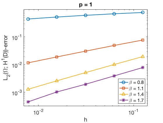
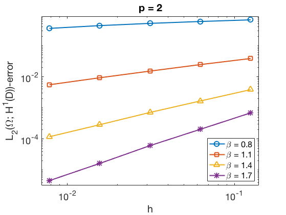
Figure 1. Observed errors of the field in $L_{2}(\Omega;L_{2}(\mathcal{D}))$ (top), $L_{1}(\Omega;L_{\infty}(\mathcal{D}))$ (middle) and $L_{2}(\Omega;H^{1}_{0}(\mathcal{D}))$ (bottom) for polynomial degree $p\in\{1,2\}$ (left, right), and different values of $\beta$, shown in a log-log scale as a function of the mesh width $h$. The corresponding observed convergence rates are shown in Table 2.

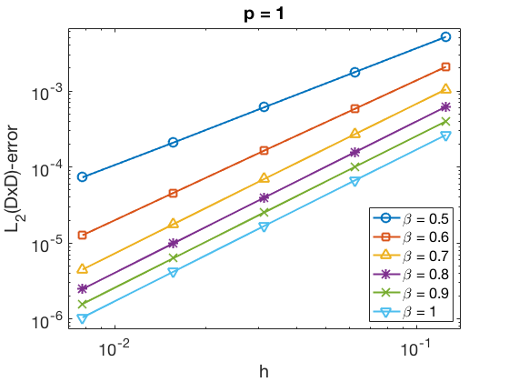
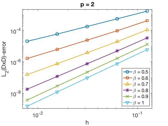
Figure 2. Observed $L_{q}(\mathcal{D}\times\mathcal{D})$-error of the covariance function for $q\in\{2,\infty\}$ (top, bottom), polynomial degree $p\in\{1,2\}$ (left, right), and different values of $\beta$, shown in a log-log scale as a function of the mesh width $h$. The corresponding observed convergence rates are shown in Table 2.

The resulting observed errors are displayed in Figure 1 for the fields and in Figure 2 for the covariances. Overall, the empirical results validate our theoretical outcomes fairly well, with a slight deviation for the $L_{\infty}$-studies which may be caused by a larger pre-asymptotic range.

8. Conclusion and discussion

We have identified necessary and sufficient conditions for square-integrability, Sobolev regularity, and Hölder continuity (in $L_{q}(\Omega)$-sense) for GRFs in terms of their color, as well as square-integrability, mixed Sobolev regularity, and continuity of their covariance functions, see Propositions 3.4, 3.6 and 3.7. Subsequently, we have applied these findings to generalized Whittle–Matérn fields, see $\mathcal{Z}^{\beta}$ in (4.1), where these conditions become assumptions on the smoothness parameter $\beta>0$, corresponding to the fractional exponent of the color $L^{-\beta}$, see Lemmata 4.1–4.3.

While these regularity results readily implied convergence of spectral Galerkin approximations, see Corollaries 5.1–5.3, significantly more work was needed to derive convergence for general Galerkin (such as finite element) approximations, for the following reason: It was unknown, how the deterministic fractional Galerkin error $L^{-\beta}g-L_{h}^{-\beta}g$ behaves in the Sobolev space $H^{\sigma}(\mathcal{D})$, for $0\leq\sigma\leq 1$, all possible exponents $\beta>0$, and sources $g\in H^{\delta}(\mathcal{D})$ of possibly negative regularity $\delta<0$. We have identified this behavior in Theorem 6.6 for the general situation that the second-order elliptic differential operator $L$ is $H^{1+\alpha}(\mathcal{D})$-regular for some $0<\alpha\leq 1$. This result could be exploited to show convergence of the sinc-Galerkin approximations and their covariances to the Whittle–Matérn field $\mathcal{Z}^{\beta}$ and to its covariance function $\varrho^{\beta}$, respectively, see Theorems 6.18 and 6.23.

The fact that the Rayleigh–Ritz projection and, thus, the deterministic Galerkin error $L^{-1}g-L_{h}^{-1}g$ converges at the rate $\min\{1+\alpha-\sigma,\,2\alpha\}$ in $H^{\sigma}(\mathcal{D})$, $0\leq\sigma\leq 1$, if $L$ is $H^{1+\alpha}(\mathcal{D})$-regular, cf. Lemma 6.3, and at the rate $p+1-\sigma$ if the problem is “smooth” and a conforming finite element discretization with piecewise polynomial basis functions of degree at most $p\in\mathbb{N}$ is used, combined with the low regularity of white noise in $\dot{H}^{-\nicefrac{{d}}{{2}}-\varepsilon}_{L}$, show that the Sobolev convergence rates of Theorems 6.18 and 6.23 are (essentially, up to $\varepsilon>0$) optimal. In addition, we believe that our results on Hölder convergence of the field and on $L_{\infty}$-convergence of the covariance function for $d=1$ in Theorem 6.23 are optimal (i) if the problem is only $H^{1+\alpha}(\mathcal{D})$-regular for $\alpha\in(0,1)$ maximal, or (ii) if the problem is smooth and $\beta\in(\nicefrac{{1}}{{4}},1)$ (resp. $\beta\in(\nicefrac{{1}}{{4}},\nicefrac{{5}}{{8}})$ for the covariance). However, the deterministic $p$-FEM $L_{\infty}$-rate for $d=1$ is known to be $p+1$ if the problem is smooth, see [14]. Thus, our results will not be sharp in this case, see also our numerical experiments in Section 7.

Since the approach on deriving optimal $L_{\infty}$-rates involves non-Hilbertian regularity of the solution in $W^{p+1,\infty}(\mathcal{D})$, such a discussion was beyond the scope of this article and we leave this problem as well as the $C^{\delta}(\overline{\mathcal{D}})\,$/$\,L_{\infty}(\mathcal{D}\times\mathcal{D})$ error analysis of sinc-Galerkin approximations in dimension $d\in\{2,3\}$ as topics for future research.

Appendix A Proof of Proposition 6.13

The following lemma will be the main tool for the derivation of Proposition 6.13.

Lemma A.1.

Suppose Assumptions 2.1.I–II and 6.1.III. Let Assumption 6.1.IV be fulfilled with parameters $r,s_{0},t>0$ such that $\nicefrac{{r}}{{2}}\geq t-1$ and $s_{0}\geq t$. Let $d\in\mathbb{N}$, $\beta>0$, and $\rho_{0}(\,\cdot)$, $\rho_{1}(\,\cdot\,)$ be as in (6.33), i.e.,

$$\rho_{0}(\tau) :=\min\left\{r,\,s_{0},\,2\beta+\tau-\nicefrac{{d}}{{2}}\right\},\quad\rho_{1}(\tau):=\min\left\{\nicefrac{{r}}{{2}},\,s_{0},\,2\beta-1+\tau-\nicefrac{{d}}{{2}}\right\},$$

and define the exception set

$$\mathcal{E}_{\tau}:=\left\{2(t-1)-2\beta+\sigma+\nicefrac{{d}}{{2}},\,t-2\beta+\sigma+\nicefrac{{d}}{{2}}:\sigma\in\{0,1\}\right\}.$$

Then, for $\sigma\in\{0,1\}$, the Galerkin error $\widetilde{E}_{V_{h}}^{\beta}$ in (6.22) satisfies

$$\sum_{j\in\mathbb{N}}\lambda_{j}^{-\tau}\bigl{\|}\widetilde{E}_{V_{h}}^{\beta}e_{j}\bigr{\|}_{\sigma}^{2}\lesssim_{(C_{0},C_{\lambda},\sigma,\tau,\beta,A,\kappa,\mathcal{D})}C_{\tau,h}h^{2\rho_{\sigma}(\tau)}\qquad\forall\tau\geq 0,$$ (A.1)

for sufficiently small $h>0$. Here, $\{(\lambda_{j},e_{j})\}_{j\in\mathbb{N}}$ are the $L_{2}(\mathcal{D})$-orthonormal, ordered eigenpairs of $L$ in (2.2) and we set $C_{\tau,h}:=1$ if $\tau\not\in\mathcal{E}_{\tau}$ and $C_{\tau,h}:=\ln(1/h)$ if $\tau\in\mathcal{E}_{\tau}$.

Proof.

Fix $\tau\geq 0$. The definitions of $\widetilde{E}_{V_{h}}^{\beta}$ in (6.22) and of $\widetilde{\Pi}_{h}$ in (6.18) yield

$$\sum_{j\in\mathbb{N}}\lambda_{j}^{-\tau}\bigl{\|}\widetilde{E}_{V_{h}}^{\beta}e_{j}\bigr{\|}_{\sigma}^{2} =\sum_{j=1}^{N_{h}}\lambda_{j}^{-\tau}\bigl{\|}\lambda_{j}^{-\beta}e_{j}-\lambda_{j,h}^{-\beta}e_{j,h}\bigr{\|}_{\sigma}^{2}$$

$$\lesssim\sum_{j=1}^{N_{h}}\lambda_{j}^{-\tau+\sigma}\bigl{|}\lambda_{j}^{-\beta}-\lambda_{j,h}^{-\beta}\bigr{|}^{2}+\sum_{j=1}^{N_{h}}\lambda_{j}^{-\tau}\lambda_{j,h}^{-2\beta}\|e_{j}-e_{j,h}\|_{\sigma}^{2}.$$ (A.2)

By the mean value theorem, $\lambda_{j}^{-\beta}-\lambda_{j,h}^{-\beta}=\widetilde{\lambda}_{j}^{-\beta-1}(\lambda_{j,h}-\lambda_{j})$ for some $\widetilde{\lambda}_{j}\in(\lambda_{j},\lambda_{j,h})$. Thus, we can use (6.5) from Assumption 6.1.IV and the spectral behavior (2.3) from Lemma 2.2 combined with Assumption 6.1.III to bound the first sum in (A.2),

$$\sum_{j=1}^{N_{h}}\lambda_{j}^{-\tau+\sigma}\bigl{|}\lambda_{j}^{-\beta}-\lambda_{j,h}^{-\beta}\bigr{|}^{2} \leq C_{\lambda}^{2}h^{2r}\sum_{j=1}^{N_{h}}\lambda_{j}^{-2\beta-\tau+\sigma+2(t-1)}$$

$$\lesssim_{(C_{\lambda},\sigma,\tau,\beta,A,\kappa,\mathcal{D})}C_{\tau,h}h^{2\min\left\{r,\,2\beta-\sigma+\tau-\nicefrac{{d}}{{2}}\right\}}.$$ (A.3)

where we also have used that $r\geq 2(t-1)$ by assumption. For the second sum in (A.2) we distinguish the cases $\sigma=0$ and $\sigma=1$. If $\sigma=0$, we can apply (6.6) of Assumption 6.1.IV and obtain

$$\sum_{j=1}^{N_{h}}\lambda_{j}^{-\tau}\lambda_{j,h}^{-2\beta}\|e_{j}-e_{j,h}\|_{0}^{2} \leq C_{0}h^{2s_{0}}\sum_{j=1}^{N_{h}}\lambda_{j}^{-2\beta-\tau+t}$$

$$\lesssim_{(C_{0},\sigma,\tau,\beta,A,\kappa,\mathcal{D})}C_{\tau,h}h^{2\min\left\{s_{0},\,2\beta+\tau-\nicefrac{{d}}{{2}}\right\}},$$ (A.4)

since $s_{0}\geq t$. For $\sigma=1$, we first note that (6.5)–(6.6) of Assumption 6.1.IV imply the following estimate with respect to the norm on $\dot{H}^{1}_{L}$,

$$\|e_{j}-e_{j,h}\|_{1}^{2}=\lambda_{j}\|e_{j}-e_{j,h}\|_{0}^{2}+\lambda_{j,h}-\lambda_{j}\leq C_{0}h^{2s_{0}}\lambda_{j}^{t+1}+C_{\lambda}h^{r}\lambda_{j}^{t}.$$

Here, we have used the identity $(e_{j},e_{j,h})_{1}=\lambda_{j}(e_{j},e_{j,h})_{0}$. Thus, if $\sigma=1$, we can bound the second sum in (A.2) as follows,

$$\sum_{j=1}^{N_{h}}\lambda_{j}^{-\tau}\lambda_{j,h}^{-2\beta} \|e_{j}-e_{j,h}\|_{1}^{2}\leq C_{0}h^{2s_{0}}\sum_{j=1}^{N_{h}}\lambda_{j}^{-2\beta-\tau+t+1}+C_{\lambda}h^{r}\sum_{j=1}^{N_{h}}\lambda_{j}^{-2\beta-\tau+t}$$

$$\lesssim_{(C_{0},C_{\lambda},\sigma,\tau,\beta,A,\kappa,\mathcal{D})}C_{\tau,h}h^{2\min\left\{\nicefrac{{r}}{{2}},\,s_{0},\,2\beta-1+\tau-\nicefrac{{d}}{{2}}\right\}},$$ (A.5)

since $s_{0}\geq t$ and $\nicefrac{{r}}{{2}}\geq t-1$ by assumption. Combining (A.2), (A.3), (A.4) and (A.5) completes the proof. ∎

Proof of Proposition 6.13.

In order to derive (6.35), we start with splitting the error in the norm $\|\,\cdot\,\|_{\sigma}$ on $\dot{H}^{\sigma}_{L}$, cf. (2.4), which by (2.6) of Lemma 2.4 implies an upper bound for the Sobolev norm:

$$\left(\mathbb{E}\left[\bigl{\|}\mathcal{Z}^{\beta}-\widetilde{\mathcal{Z}}^{\beta}_{h,k}\bigr{\|}_{\sigma}^{q}\right]\right)^{\nicefrac{{1}}{{q}}} \leq\left(\mathbb{E}\left[\bigl{\|}\mathcal{Z}^{\beta}-\mathcal{Z}^{\beta}_{N_{h}}\bigr{\|}_{\sigma}^{q}\right]\right)^{\nicefrac{{1}}{{q}}}+\left(\mathbb{E}\left[\bigl{\|}\mathcal{Z}^{\beta}_{N_{h}}-\widetilde{\mathcal{Z}}^{\beta}_{h}\bigr{\|}_{\sigma}^{q}\right]\right)^{\nicefrac{{1}}{{q}}}$$

$$\quad+\left(\mathbb{E}\left[\bigl{\|}\widetilde{\mathcal{Z}}^{\beta}_{h}-\widetilde{\mathcal{Z}}^{\beta}_{h,k}\bigr{\|}_{\sigma}^{q}\right]\right)^{\nicefrac{{1}}{{q}}}=:\text{($\text{A}_{\mathcal{Z}}$)}+\text{($\text{B}_{\mathcal{Z}}$)}+\text{($\text{C}_{\mathcal{Z}}$)}.$$

Here, $\mathcal{Z}^{\beta}_{N_{h}}$ is the spectral Galerkin approximation from (5.1) and $\widetilde{\mathcal{Z}}^{\beta}_{h}$ denotes a GRF colored by $L_{h}^{-\beta}\widetilde{\Pi}_{h}$. We readily obtain a bound for ($\text{A}_{\mathcal{Z}}$) from (5.3) of Corollary 5.1, combined with Assumption 6.1.III. This gives

$$\text{($\text{A}_{\mathcal{Z}}$)}\lesssim_{(q,\sigma,\beta,A,\kappa,\mathcal{D})}N_{h}^{-\nicefrac{{1}}{{d}}\,\left(2\beta-\sigma-\nicefrac{{d}}{{2}}\right)}\lesssim_{(q,\sigma,\beta,A,\kappa,\mathcal{D})}h^{2\beta-\sigma-\nicefrac{{d}}{{2}}}.$$

Note that it suffices to estimate the terms ($\text{B}_{\mathcal{Z}}$) and ($\text{C}_{\mathcal{Z}}$) for $\sigma\in\{0,1\}$. The respective bounds for $\sigma\in(0,1)$ then follow by interpolation. By definition of the Galerkin and the quadrature error, $\widetilde{E}_{V_{h}}^{\beta}$, $\widetilde{E}_{Q}^{\beta}$, in (6.22)–(6.23) and by Proposition 3.7,

$$\text{($\text{B}_{\mathcal{Z}}$)}\lesssim_{q}\bigl{\|}\widetilde{E}_{V_{h}}^{\beta}\bigr{\|}_{\mathcal{L}_{2}^{0;\sigma}}\quad\text{and}\quad\text{($\text{C}_{\mathcal{Z}}$)}\lesssim_{q}\bigl{\|}\widetilde{E}_{Q}^{\beta}\bigr{\|}_{\mathcal{L}_{2}^{0;\sigma}},\qquad\mathcal{L}_{2}^{\theta;\sigma}:=\mathcal{L}_{2}\bigl{(}\dot{H}^{\theta}_{L};\dot{H}^{\sigma}_{L}\bigr{)}.$$

Since we have to consider these terms only for $\sigma\in\{0,1\}$, the first term can be bounded by (A.1) of Lemma A.1 (with $\tau:=0$),

$$\text{($\text{B}_{\mathcal{Z}}$)}^{2} \lesssim_{q}\bigl{\|}\widetilde{E}_{V_{h}}^{\beta}\bigr{\|}_{\mathcal{L}_{2}^{0;\sigma}}^{2}=\sum_{j\in\mathbb{N}}\bigl{\|}\widetilde{E}_{V_{h}}^{\beta}e_{j}\bigr{\|}_{\sigma}^{2}\lesssim_{(C_{0},C_{\lambda},\sigma,\beta,A,\kappa,\mathcal{D})}\left(C_{\beta,h}^{\mathcal{Z}}\right)^{2}h^{2\rho_{\sigma}(0)}.$$

where $C_{\beta,h}^{\mathcal{Z}}>0$ is defined as in the statement of Proposition 6.13. To estimate ($\text{C}_{\mathcal{Z}}$), we first apply the convergence result of the sinc quadrature from [5, Lem. 3.4, Rem. 3.1, Thm. 3.5]. Thus, for sufficiently small $k>0$ and all $1\leq j\leq N_{h}$,

$$\bigl{\|}\widetilde{E}_{Q}^{\beta}e_{j}\bigr{\|}_{L_{2}(\mathcal{D})}=\bigl{\|}\bigl{(}L_{h}^{-\beta_{\star}}-Q_{h,k}^{\beta_{\star}}\bigr{)}L_{h}^{-n_{\beta}}e_{j,h}\bigr{\|}_{L_{2}(\mathcal{D})}\lesssim_{(\beta,A,\kappa,\mathcal{D})}e^{-\nicefrac{{\pi^{2}}}{{(2k)}}}\lambda_{j,h}^{-n_{\beta}}.$$

Again by equivalence of the norms $\|\,\cdot\,\|_{\sigma}$, $\|\,\cdot\,\|_{H^{\sigma}(\mathcal{D})}$ for $\sigma\in\{0,1\}$, see Lemma 2.4, and by the inverse inequality (6.4) from Assumption 6.1.II, we then find

$$\text{($\text{C}_{\mathcal{Z}}$)}^{2} \lesssim_{q}\bigl{\|}\widetilde{E}_{Q}^{\beta}\bigr{\|}_{\mathcal{L}_{2}^{0;\sigma}}^{2}=\sum_{j=1}^{N_{h}}\bigl{\|}\widetilde{E}_{Q}^{\beta}e_{j}\bigr{\|}_{\sigma}^{2}\lesssim_{(\sigma,A,\kappa,\mathcal{D})}h^{-2\sigma}\sum_{j=1}^{N_{h}}\bigl{\|}\widetilde{E}_{Q}^{\beta}e_{j}\bigr{\|}_{L_{2}(\mathcal{D})}^{2}$$

$$\lesssim_{(q,\sigma,\beta,A,\kappa,\mathcal{D})}e^{-\nicefrac{{\pi^{2}}}{{k}}}h^{-2\sigma}\sum_{j=1}^{N_{h}}\lambda_{j,h}^{-2n_{\beta}}\lesssim_{(q,\sigma,\beta,A,\kappa,\mathcal{D})}e^{-\nicefrac{{\pi^{2}}}{{k}}}h^{-2\sigma-d\,\mathds{1}_{\{\beta<1\}}},$$

where we have used the spectral behavior (2.3) from Lemma 2.2 and Assumptions 6.1.III-IV in the last step. This completes the proof of (6.35).

We now proceed with the derivation of (6.36). To this end, we consider the error with respect to the norm $\|\,\cdot\,\|_{\sigma,\sigma}$, see (3.15), since the embedding in (2.6) implies that $\dot{H}^{\sigma,\sigma}_{L}\hookrightarrow H^{\sigma,\sigma}(\mathcal{D}\times\mathcal{D})$. We again partition the error in three terms,

$$\bigl{\|}\varrho^{\beta}-\widetilde{\varrho}^{\beta}_{h,k}\bigr{\|}_{\sigma,\sigma} \leq\bigl{\|}\varrho^{\beta}-\varrho^{\beta}_{N_{h}}\bigr{\|}_{\sigma,\sigma}+\bigl{\|}\varrho^{\beta}_{N_{h}}-\widetilde{\varrho}^{\beta}_{h}\bigr{\|}_{\sigma,\sigma}+\bigl{\|}\widetilde{\varrho}^{\beta}_{h}-\widetilde{\varrho}^{\beta}_{h,k}\bigr{\|}_{\sigma,\sigma}$$

$$=:\text{($\text{A}_{\varrho}$)}+\text{($\text{B}_{\varrho}$)}+\text{($\text{C}_{\varrho}$)},$$

where $\widetilde{\varrho}^{\beta}_{h}$ denotes the covariance function of the above-introduced GRF $\widetilde{\mathcal{Z}}^{\beta}_{h}$ colored by $L_{h}^{-\beta}\widetilde{\Pi}_{h}$. A bound for the truncation error is given by (5.4) in Proposition 5.1,

$$\text{($\text{A}_{\varrho}$)}\lesssim_{(\sigma,\beta,A,\kappa,\mathcal{D})}N_{h}^{\nicefrac{{1}}{{d}}\,\left(4\beta-2\sigma-\nicefrac{{d}}{{2}}\right)}\lesssim_{(\sigma,\beta,A,\kappa,\mathcal{D})}h^{4\beta-2\sigma-\nicefrac{{d}}{{2}}},$$

where we also used Assumption 6.1.III. We bound the remaining terms ($\text{B}_{\varrho}$) and ($\text{C}_{\varrho}$) for $\sigma\in\{0,1\}$. Since $\bigl{[}\dot{H}^{0,0}_{L},\dot{H}^{1,1}_{L}\bigr{]}_{\sigma}=\dot{H}^{\sigma,\sigma}_{L}$, see [41, Thm. 16.1], we may again interpolate these results for $\sigma\in(0,1)$. To this end, we first exploit (3.20) from Proposition 3.7 and (6.31) to derive for ($\text{B}_{\varrho}$) that

($$\text{B}_{\varrho} =\bigl{\|}L_{N_{h}}^{-2\beta}-L_{h}^{-\beta}\widetilde{\Pi}_{h}\bigl{(}L_{h}^{-\beta}\widetilde{\Pi}_{h}\bigr{)}^{*}\bigr{\|}_{\mathcal{L}_{2}^{-\sigma;\sigma}}\leq\bigl{\|}\widetilde{E}_{V_{h}}^{\beta}\bigl{(}L_{N_{h}}^{-\beta}+L_{h}^{-\beta}\widetilde{\Pi}_{h}\bigr{)}^{*}\bigr{\|}_{\mathcal{L}_{2}^{-\sigma;\sigma}}$$)

$$\leq\bigl{\|}\widetilde{E}_{V_{h}}^{\beta}L_{N_{h}}^{-\beta}\bigr{\|}_{\mathcal{L}_{2}^{-\sigma;\sigma}}+\bigl{\|}\widetilde{E}_{V_{h}}^{\beta}\bigl{(}L_{h}^{-\beta}\widetilde{\Pi}_{h}\bigr{)}^{*}\bigr{\|}_{\mathcal{L}_{2}^{-\sigma;\sigma}}=:\text{($\text{B}^{\prime}_{\varrho}$)}+\text{($\text{B}^{\prime\prime}_{\varrho}$)}.$$

By Lemma A.1 (for $\tau:=2\beta-\sigma>\nicefrac{{d}}{{2}}>0$ in (A.1)) we have, for $\sigma\in\{0,1\}$ and for $C_{\beta,h}^{\varrho}>0$ as in the statement of Proposition 6.13,

$$\text{($\text{B}^{\prime}_{\varrho}$)}^{2} =\sum_{j\in\mathbb{N}}\lambda_{j}^{-(2\beta-\sigma)}\bigl{\|}\widetilde{E}_{V_{h}}^{\beta}e_{j}\bigr{\|}_{\sigma}^{2}\lesssim_{(C_{0},C_{\lambda},\sigma,\beta,A,\kappa,\mathcal{D})}\bigl{(}C_{\beta,h}^{\varrho}\bigr{)}^{2}h^{2\rho_{\sigma}(2\beta-\sigma)}.$$

Next, we use the identity $\bigl{(}L_{h}^{-\beta}\widetilde{\Pi}_{h}\bigr{)}^{*}e_{j}=\sum_{\ell=1}^{N_{h}}\lambda_{\ell,h}^{-\beta}(e_{j},e_{\ell,h})_{L_{2}(\mathcal{D})}\,e_{\ell}$, the orthogonality $(e_{k,h},e_{\ell,h})_{\sigma}=\delta_{k\ell}\lambda_{k,h}^{\sigma}$ (here, $\delta_{k\ell}$ denotes the Kronecker delta), which holds for $\sigma\in\{0,1\}$, and the relation $\lambda_{j}\leq\lambda_{j,h}$ from Assumption 6.1.IV. With these steps, we obtain again by (A.1) of Lemma A.1 (with $\tau:=2\beta-\sigma$) a bound for ($\text{B}^{\prime\prime}_{\varrho}$),

$$\text{($\text{B}^{\prime\prime}_{\varrho}$)}^{2} =\sum_{j\in\mathbb{N}}\sum_{i=1}^{N_{h}}\sum_{\ell=1}^{N_{h}}\lambda_{j}^{\sigma}\lambda_{i,h}^{-\beta}\lambda_{\ell,h}^{-\beta}(e_{j},e_{i,h})_{L_{2}(\mathcal{D})}(e_{j},e_{\ell,h})_{L_{2}(\mathcal{D})}\bigl{(}\widetilde{E}_{V_{h}}^{\beta}e_{i},\widetilde{E}_{V_{h}}^{\beta}e_{\ell}\bigr{)}_{\sigma}$$

$$=\sum_{i=1}^{N_{h}}\sum_{\ell=1}^{N_{h}}\lambda_{i,h}^{-\beta}\lambda_{\ell,h}^{-\beta}(e_{i,h},e_{\ell,h})_{\sigma}\bigl{(}\widetilde{E}_{V_{h}}^{\beta}e_{i}\widetilde{E}_{V_{h}}^{\beta}e_{\ell}\bigr{)}_{\sigma}=\sum_{\ell=1}^{N_{h}}\lambda_{\ell,h}^{-(2\beta-\sigma)}\bigl{\|}\widetilde{E}_{V_{h}}^{\beta}e_{\ell}\bigr{\|}_{\sigma}^{2}$$

$$\leq\sum_{\ell\in\mathbb{N}}\lambda_{\ell}^{-(2\beta-\sigma)}\bigl{\|}\widetilde{E}_{V_{h}}^{\beta}e_{\ell}\bigr{\|}_{\sigma}^{2}\lesssim_{(C_{0},C_{\lambda},\sigma,\beta,A,\kappa,\mathcal{D})}\bigl{(}C_{\beta,h}^{\varrho}\bigr{)}^{2}h^{2\rho_{\sigma}(2\beta-\sigma)}.$$

In conclusion, $\bigl{\|}\varrho_{N_{h}}^{\beta}-\widetilde{\varrho}_{h}^{\beta}\bigr{\|}_{\sigma,\sigma}\leq\text{($\text{B}^{\prime}_{\varrho}$)}+\text{($\text{B}^{\prime\prime}_{\varrho}$)}\lesssim_{(C_{0},C_{\lambda},\sigma,\beta,A,\kappa,\mathcal{D})}\bigl{(}C_{\beta,h}^{\varrho}\bigr{)}^{2}h^{\rho_{\sigma}(2\beta-\sigma)}$ for $\sigma\in\{0,1\}$. For ($\text{C}_{\varrho}$), we derive with the equivalence of the norms $\|\,\cdot\,\|_{\sigma}$, $\|\,\cdot\,\|_{H^{\sigma}(\mathcal{D})}$, the inverse inequality (6.4) from Assumption 6.1.II, and the convergence result for the sinc quadrature [5, Lem. 3.4, Rem. 3.1, Thm. 3.5] the following, if $\sigma\in\{0,1\}$,

$$\text{($\text{C}_{\varrho}$)}^{2} \lesssim_{(\sigma,A,\kappa,\mathcal{D})}h^{-2\sigma}\sum_{j\in\mathbb{N}}\lambda_{j}^{\sigma}\bigl{\|}\widetilde{E}_{Q}^{\beta}\bigl{(}L_{h}^{-\beta}\widetilde{\Pi}_{h}+Q_{h,k}^{\beta_{\star}}L_{h}^{-n_{\beta}}\widetilde{\Pi}_{h}\bigr{)}^{*}e_{j}\bigr{\|}_{L_{2}(\mathcal{D})}^{2}$$

$$\lesssim_{(\sigma,\beta,A,\kappa,\mathcal{D})}e^{-\nicefrac{{\pi^{2}}}{{k}}}h^{-2\sigma}\sum_{j\in\mathbb{N}}\lambda_{j}^{\sigma}\bigl{\|}L_{h}^{-n_{\beta}}\widetilde{\Pi}_{h}\widetilde{\Pi}_{h}^{*}(L_{h}^{-n_{\beta}})^{*}\bigl{(}L_{h}^{-\beta_{\star}}+Q_{h,k}^{\beta_{\star}}\bigr{)}^{*}e_{j}\bigr{\|}_{L_{2}(\mathcal{D})}^{2}.$$

Since $L_{h}^{-n_{\beta}}\widetilde{\Pi}_{h}\widetilde{\Pi}_{h}^{*}(L_{h}^{-n_{\beta}})^{*}e_{\ell,h}=\lambda_{\ell,h}^{-2n_{\beta}}e_{\ell,h}$ for all $\ell\in\{1,\ldots,N_{h}\}$, this shows that

$$\text{($\text{C}_{\varrho}$)}^{2} \lesssim_{(\sigma,\beta,A,\kappa,\mathcal{D})}e^{-\nicefrac{{\pi^{2}}}{{k}}}h^{-2\sigma}\sum_{\ell=1}^{N_{h}}\sum_{j\in\mathbb{N}}\lambda_{j}^{\sigma}\lambda_{\ell,h}^{-4n_{\beta}}\bigl{(}e_{j},\bigl{(}L_{h}^{-\beta_{\star}}+Q_{h,k}^{\beta_{\star}}\bigr{)}e_{\ell,h}\bigr{)}_{L_{2}(\mathcal{D})}^{2}.$$

Next, again by the inverse inequality (6.4) we find

$$\text{($\text{C}_{\varrho}$)}^{2} \lesssim_{(\sigma,\beta,A,\kappa,\mathcal{D})}e^{-\nicefrac{{\pi^{2}}}{{k}}}h^{-4\sigma}\sum_{\ell=1}^{N_{h}}\lambda_{\ell,h}^{-4n_{\beta}}\bigl{\|}\bigl{(}L_{h}^{-\beta_{\star}}+Q_{h,k}^{\beta_{\star}}\bigr{)}e_{\ell,h}\bigr{\|}_{L_{2}(\mathcal{D})}^{2}$$

$$\lesssim_{(\sigma,\beta,A,\kappa,\mathcal{D})}e^{-\nicefrac{{\pi^{2}}}{{k}}}h^{-4\sigma}\sum_{\ell=1}^{N_{h}}\lambda_{\ell}^{-4n_{\beta}}\lesssim_{(\sigma,\beta,A,\kappa,\mathcal{D})}e^{-\pi^{2}/k}h^{-4\sigma-d\,\mathds{1}_{\{\beta<1\}}}.$$

Here, we have used the uniform stability of $L^{-\beta_{\star}}$, $Q_{h,k}^{\beta_{\star}}$ with respect to $h$ and $k$, see (6.32), as well as (2.3) from Lemma 2.2 and Assumption 6.1.I. Combining the bounds for ($\text{A}_{\varrho}$), ($\text{B}_{\varrho}$), ($\text{C}_{\varrho}$) completes the proof. ∎

References

• [1] R. Andreev, ppfem – MATLAB routines for the FEM with piecewise polynomial splines on product meshes, 2016. https://bitbucket.org/numpde/ppfem/, downloaded on November 12, 2018.
• [2] D. Bolin, K. Kirchner, and M. Kovács, Numerical solution of fractional elliptic stochastic PDEs with spatial white noise, IMA J. Numer. Anal., (2018). Electronic.
• [3] D. Bolin, K. Kirchner, and M. Kovács, Weak convergence of Galerkin approximations for fractional elliptic stochastic PDEs with spatial white noise, BIT, 58 (2018), pp. 881–906.
• [4] D. Bolin and F. Lindgren, Spatial models generated by nested stochastic partial differential equations, with an application to global ozone mapping, Ann. Appl. Stat., 5 (2011), pp. 523–550.
• [5] A. Bonito and J. E. Pasciak, Numerical approximation of fractional powers of elliptic operators, Math. Comp., 84 (2015), pp. 2083–2110.
• [6] J. H. Bramble, J. E. Pasciak, and O. Steinbach, On the stability of the $L^{2}$ projection in $H^{1}(\Omega)$, Math. Comp., 71 (2002), pp. 147–156.
• [7] M. Cameletti, F. Lindgren, D. Simpson, and H. Rue, Spatio-temporal modeling of particulate matter concentration through the SPDE approach, AStA Adv. Stat. Anal., 97 (2013), pp. 109–131.
• [8] G. Chan and A. T. A. Wood, Algorithm AS 312: An algorithm for simulating stationary Gaussian random fields, J. Roy. Statist. Soc. Ser. C, 46 (1997), pp. 171–181.
• [9] J. Chen and M. L. Stein, Linear-cost covariance functions for Gaussian random fields. Preprint, arXiv:1711.05895, 2017.
• [10] M. Crouzeix and V. Thomée, The stability in $L_{p}$ and $W^{1}_{p}$ of the $L_{2}$-projection onto finite element function spaces, Math. Comp., 48 (1987), pp. 521–532.
• [11] E. B. Davies, Spectral theory and differential operators, vol. 42 of Cambridge Studies in Advanced Mathematics, Cambridge University Press, Cambridge, 1995.
• [12] E. Di Nezza, G. Palatucci, and E. Valdinoci, Hitchhiker’s guide to the fractional Sobolev spaces, Bull. Sci. Math., 136 (2012), pp. 521–573.
• [13] C. R. Dietrich and G. N. Newsam, Fast and exact simulation of stationary Gaussian processes through circulant embedding of the covariance matrix, SIAM J. Sci. Comput., 18 (1997), pp. 1088–1107.
• [14] J. Douglas, Jr., T. Dupont, and L. Wahlbin, Optimal $L_{\infty}$ error estimates for Galerkin approximations to solutions of two-point boundary value problems, Math. Comp., 29 (1975), pp. 475–483.
• [15] A. Ern and J.-L. Guermond, Theory and practice of finite elements, vol. 159 of Applied Mathematical Sciences, Springer-Verlag, New York, 2004.
• [16] L. C. Evans, Partial differential equations, vol. 19 of Graduate Studies in Mathematics, American Mathematical Society, Providence, RI, second ed., 2010.
• [17] M. Feischl, F. Y. Kuo, and I. H. Sloan, Fast random field generation with H-matrices, Numer. Math., 140 (2018), pp. 639–676.
• [18] D. Gilbarg and N. S. Trudinger, Elliptic partial differential equations of second order, Classics in Mathematics, Springer-Verlag, Berlin, 2001. Reprint of the 1998 edition.
• [19] I. G. Graham, F. Y. Kuo, D. Nuyens, R. Scheichl, and I. H. Sloan, Analysis of circulant embedding methods for sampling stationary random fields, SIAM J. Numer. Anal., 56 (2018), pp. 1871–1895.
• [20] P. Grisvard, Caractérisation de quelques espaces d’interpolation, Arch. Rational Mech. Anal., 25 (1967), pp. 40–63.
• [21] P. Grisvard, Elliptic problems in nonsmooth domains, vol. 69 of Classics in Applied Mathematics, Society for Industrial and Applied Mathematics (SIAM), Philadelphia, PA, 2011.
• [22] J.-L. Guermond, The LBB condition in fractional Sobolev spaces and applications, IMA J. Numer. Anal., 29 (2009), pp. 790–805.
• [23] N. Hale, N. J. Higham, and L. N. Trefethen, Computing ${\bf A}^{\alpha},\ \log({\bf A})$, and related matrix functions by contour integrals, SIAM J. Numer. Anal., 46 (2008), pp. 2505–2523.
• [24] J. Latz, M. Eisenberger, and E. Ullmann, Fast sampling of parameterised Gaussian random fields, Comput. Methods Appl. Mech. Engrg., 348 (2019), pp. 978–1012.
• [25] M. Ledoux and M. Talagrand, Probability in Banach spaces, Classics in Mathematics, Springer-Verlag, Berlin, 2011. Isoperimetry and processes, Reprint of the 1991 edition.
• [26] F. Lindgren, H. v. Rue, and J. Lindström, An explicit link between Gaussian fields and Gaussian Markov random fields: the stochastic partial differential equation approach, J. R. Stat. Soc. Ser. B Stat. Methodol., 73 (2011), pp. 423–498. With discussion.
• [27] A. Lunardi, Interpolation theory, vol. 16 of Appunti. Scuola Normale Superiore di Pisa (Nuova Serie), Edizioni della Normale, Pisa, 2018.
• [28] K. Mittmann and I. Steinwart, On the existence of continuous modifications of vector-valued random fields, Georgian Math. J., 10 (2003), pp. 311–317.
• [29] D. Nualart, The Malliavin calculus and related topics, Probability and its Applications (New York), Springer-Verlag, Berlin, second ed., 2006.
• [30] S. Osborn, P. S. Vassilevski, and U. Villa, A multilevel, hierarchical sampling technique for spatially correlated random fields, SIAM J. Sci. Comput., 39 (2017), pp. S543–S562.
• [31] E.-M. Ouhabaz, Analysis of heat equations on domains, vol. 31 of London Mathematical Society Monographs Series, Princeton University Press, Princeton, NJ, 2005.
• [32] A. Pazy, Semigroups of linear operators and applications to partial differential equations, vol. 44 of Applied Mathematical Sciences, Springer-Verlag, New York, 1983.
• [33] W. D. Penny, N. J. Trujillo-Barreto, and K. J. Friston, Bayesian fMRI time series analysis with spatial priors, NeuroImage, 24 (2005), pp. 350–362.
• [34] D. Revuz and M. Yor, Continuous martingales and Brownian motion, vol. 293 of Grundlehren der Mathematischen Wissenschaften, Springer-Verlag, Berlin, third ed., 1999.
• [35] S. R. Sain, R. Furrer, and N. Cressie, A spatial analysis of multivariate output from regional climate models, Ann. Appl. Stat., 5 (2011), pp. 150–175.
• [36] E. M. Stein, Singular integrals and differentiability properties of functions, Princeton Mathematical Series, No. 30, Princeton University Press, Princeton, N.J., 1970.
• [37] I. Steinwart and C. Scovel, Mercer’s theorem on general domains: on the interaction between measures, kernels, and RKHSs, Constr. Approx., 35 (2012), pp. 363–417.
• [38] G. Strang and G. Fix, An analysis of the finite element method, Wellesley-Cambridge Press, Wellesley, MA, second ed., 2008.
• [39] H. Triebel, Interpolation theory, function spaces, differential operators, vol. 18 of North-Holland Mathematical Library, North-Holland Publishing Co., Amsterdam-New York, 1978.
• [40] P. Whittle, Stochastic processes in several dimensions, Bull. Inst. Internat. Statist., 40 (1963), pp. 974–994.
• [41] A. Yagi, Abstract parabolic evolution equations and their applications, Springer Monographs in Mathematics, Springer-Verlag, Berlin, 2010.