Study of the core-crust transition in neutron stars with finite-range interactions: the dynamical method

Abstract

The properties of the core-crust transition in neutron stars are investigated using effective nuclear forces of finite-range. Special attention is paid to the so-called dynamical method for locating the transition point, which, apart from the stability of the uniform nuclear matter against clusterization, also considers contributions due to finite-size effects. In particular, contributions to the transition density and pressure from the direct and exchange energies are carefully analyzed. To this end, finite-range forces of Gogny, Modified Gogny Interaction (MDI) and Simple Effective Interaction (SEI) types are used in the numerical applications. The results from the dynamical approach are compared with those from the popular thermodynamical method that neglects the surface and Coulomb effects in the stability condition. The dependence of the core-crust transition on the stiffness of the symmetry energy of the finite-range models is also addressed. Finally, we analyze the impact of the transition point on the mass, thickness and fraction of the moment of inertia of the neutron star crust. Prominent differences in these crustal properties of the star are found between using the transition point obtained with the dynamical method or the thermodynamical method. It is concluded that the core-crust transition needs to be ascertained as precisely as possible in order to have realistic estimates of the observed phenomena where the crust plays a significant role.

I Introduction

Neutron stars (NSs) are the ultradense and compact remnants of massive stars after supernova explosions Shapiro and Teukolsky (1983); Haensel et al. (2007), which are composed of neutrons, protons, leptons and, eventually, other exotic particles. NSs are also electrically neutral objects, and their different components are distributed in such a way that they are locally in $\beta$-equilibrium. The structure of a NS consists of a solid crust at low densities encompassing a homogeneous core in liquid phase. The density is maximum at the center, several times the nuclear matter density ($\simeq$ 2.3 $\times$ 10¹⁴ g cm^-3), and decreases with the distance reaching a value of the terrestrial iron ($\simeq$ 7.5 g cm^-3) at the surface of the star. The external part of the star, i.e., its outer crust, consists of nuclei distributed in a solid body-centered-cubic (bcc) lattice permeated by a free electron gas. When the density increases, the nuclei in the crust become so neutron rich that neutrons start to drip from them. In this scenario, the lattice structure of nuclear clusters still remains, but now it is embedded in free electron and neutron gases. When the average density reaches a value about half of the nuclear matter saturation density, the lattice structure disappears due to energetic reasons and the system changes to a liquid phase. The boundary between the outer and inner crust is determined by nuclear masses, and corresponds to the neutron drip out density around $4\times 10^{11}$ g cm^-3 Rüster et al. (2006); Hempel and Schaffner-Bielich (2007). However, the transition density from the crust to the core is much more uncertain and strongly model dependent Baym et al. (1971a); Kubis (2007); Ducoin et al. (2007); Xu et al. (2009a, b, 2010); Xu and Ko (2010); Moustakidis et al. (2010); Moustakidis (2012); Seif and Basu (2014); Routray et al. (2016); Gonzalez-Boquera et al. (2017).

To determine the core-crust transition density from the crust side it is required to have a precise knowledge of the Equation of State (EOS) in this region of the star. This is a complicated task owing to the presence of neutron gas and the possible existence of complex structures in the deep layers of the inner crust, where the nuclear clusters may adopt shapes different from the spherical one (i.e., what is called “pasta phases”) in order to minimize the energy Baym et al. (1971b); Lattimer and Swesty (1991); Shen et al. (1998a, b); Douchin and Haensel (2001); Sharma et al. (2015); Carreau et al. . Therefore, it is easier to investigate the core-crust transition from the core side. To this end, one searches for the violation of the stability conditions of the homogeneous core under small amplitude oscillations, which indicates the appearance of nuclear clusters and, consequently, the transition to the inner crust. There are different ways to determine the transition density from the core side, namely the thermodynamical method Kubis (2007); Xu et al. (2009a); Moustakidis et al. (2010); Moustakidis (2012); Seif and Basu (2014); Routray et al. (2016); Gonzalez-Boquera et al. (2017), the dynamical method Baym et al. (1971b); Xu et al. (2009a, b, 2010); Xu and Ko (2010); Pethick et al. (1995); Ducoin et al. (2007), the random phase approximation Horowitz and Piekarewicz (2001a, b); Carriere et al. (2003) and the Vlasov equation method Chomaz et al. (2004); Providência et al. (2006); Ducoin et al. (2008a, b); Pais et al. (2010). In the low-density regime of the core near the crust the NS matter is composed of neutrons, protons and electrons. In the thermodynamical approach, the stability is discussed in terms of the bulk properties of the EOS by imposing mechanical and chemical stability conditions, which set the boundaries of the core in the homogeneous case. On the other hand, in the dynamical method, one introduces density fluctuations for neutrons, protons and electrons, which can be expanded in plane waves of amplitude $A_{i}$ ($i=n,p,e$) and of wavevector ${\bf k}$. These fluctuations may be induced by collisions, which transfer some momentum to the system. Following Refs. Baym et al. (1971b); Pethick et al. (1995); Ducoin et al. (2008a, b); Xu et al. (2009a) one writes the variation of the energy density generated by these fluctuations in terms of the energy curvature matrix $C^{J}$. The system is stable when the curvature matrix is convex, that is, the transition density is obtained from the condition $|C^{J}|$=0. This condition determines the dispersion relation $\omega(k)$ of the collective excitations of the system due to the perturbation and the instability will appear when this frequency $\omega(k)$ becomes imaginary. Thus, the dynamical method is more realistic than the thermodynamical approach, as it incorporates surface and Coulomb effects in the stability condition that are not taken into account in the thermodynamical method.

The dynamical method introduced in Ref. Baym et al. (1971b) assumes that the energy density functional can be expressed as a sum of a homogeneous bulk part, a inhomogeneous term depending on the gradients of the neutron and proton densities and the direct Coulomb energy. The zero-range Skyrme forces directly provide an energy density functional of this type. For these interactions, the core-crust transition density has been estimated using both the thermodynamical and dynamical methods Xu et al. (2009a). In the same reference it is found that the transition density calculated with the thermodynamical approach is always higher than the value calculated with with the dynamical method. On the other hand, an analysis Xu et al. (2009a) of the transition densities using 51 Skyrme forces shows a decreasing trend, roughly linear, when the slope of the symmetry energy at saturation (parameter $L$) increases, in agreement with previous findings Oyamatsu and Iida (2007).

The estimate of the transition density using the thermodynamical method with finite-range forces is rather straightforward, as only the energy density and its first and second derivatives with respect to the neutron and proton densities are needed Xu et al. (2009a); Gonzalez-Boquera et al. (2017); Routray et al. (2016). However, to obtain the core-crust transition density using the dynamical method with finite-range forces is more involved. This estimate has been discussed, to our knowledge, only in the particular case of the MDI interaction in Refs. Xu et al. (2009a); Xu and Ko (2010).

In the dynamical method using finite-range interactions one needs to extract the gradient corrections, which are encoded in the force but do not appear explicitly in the energy density functional in the case of finite-range interactions. To solve this problem, the authors in Ref. Xu et al. (2009a) adopted the phenomenology of approximating the gradient contributions with constant coefficients whose values are taken as the respective average values of the contributions provided by 51-Skyrme interactions. A step further in the application of the dynamical method to estimate the core-crust transition density is discussed in Ref. Xu and Ko (2010) also for the particular case of MDI interactions. In this work the authors use the density matrix (DM) expansion proposed by Negele and Vautherin Negele and Vautherin (1972, 1975) to derive a Skyrme-type energy density functional including gradient contributions, but with density-dependent coefficients. Using this functional, the authors study the core-crust transition through the stability conditions provided by the linealized Vlasov equations in NS matter.

The finite-range Gogny forces were proposed by D. Gogny almost forty years ago aimed to describe simultaneously the mean-field and the pairing field Dechargé and Gogny (1980); Berger et al. (1991); Chappert et al. (2008); Goriely et al. (2009). These interactions are well suited for dealing with the deformation properties of finite nuclei and to study fission barriers. However, Gogny interactions fail when one extrapolates to the neutron star domain Sellahewa and Rios (2014); Gonzalez-Boquera et al. (2017) in spite that in the fitting protocol of the D1N Chappert et al. (2008) and D1M Goriely et al. (2009) interactions it is imposed that they reproduce the microscopic neutron matter EOS of Friedman and Pandharipande Friedman and Pandharipande (1981). To remedy this situation we have proposed Gonzalez-Boquera et al. (2018) very recently a reparametrization procedure of the D1M Gogny force, labeled D1M^∗, able to reach a maximum neutron star mass of 2$M_{\odot}$ as required by recent astronomical observations Demorest et al. (2010); Antoniadis et al. (2013).

The so-called Modified Gogny Interactions (MDI) Das et al. (2003) were originally devised for transport calculations in heavy ion collisions, but they have also been applied to other different scenarios (see Xu et al. (2009a) and references therein), in particular to NS Xu et al. (2009a, b, 2010); Xu and Ko (2010). The MDI interactions can be rewritten as a zero-range contribution plus a finite range term with a single Yukawa form factor. The parameters of the MDI interactions are determined subject to the constraint that the momentum-dependence of its single-particle potential reproduces, as best as possible, the predictions of the Gogny interaction Das et al. (2003).

The SEI interaction is an effective nuclear force constructed with a minimum number of parameters to study the momentum and density dependence of the nuclear mean field Behera et al. (1998, 2005). This interaction has a single finite-range part, which can be of any conventional form, Gaussian, Yukawa or exponential, and two zero-range terms, one of them density-dependent, containing altogether eleven parameters. Unlike the case of effective forces such as Skyrme, Gogny or M3Y, nine of the eleven parameters of SEI are fitted using experimental or empirical constraints in nuclear matter that allow one to reproduce the behaviour of the momentum and density dependence of the nuclear matter mean field as predicted by the microscopic Dirac-Brueckner-Hartree-Fock (DBHF), Brueckner-Hartree-Fock (BHF) and variational calculations (see Behera et al. (2013) and references therein). One of the remaining two parameters is determined from the study of spin polarized matter Behera et al. (2015) and the other one along with the strength of the spin-orbit interaction, absent in nuclear matter calculations, is fitted to reproduce the experimental binding energies of 620 even-even nuclei through HFB calculations Behera et al. (1998).

Our aim in this work is to discuss again the core-crust transition in the case of finite-range interactions enlarging the types of forces analyzed by including, in addition to MDI, the Gogny and SEI interactions. On the other hand, in this work we will use a DM expansion based on the Extended Thomas-Fermi approximation that was introduced in Ref. Soubbotin and Viñas (2000). This DM expansion provides, using the Kohn-Sham method in the framework of the density functional theory and including pairing correlations, a quasi-local energy density functional. With this functional one can compute in a simple way ground-state properties of finite nuclei in excellent agreement with the predictions of the full Hartree-Fock-Bogoliubov (HFB) calculations using finite-range interactions Soubbotin et al. (2003); Krewald et al. (2006); Behera et al. (2016). The paper is organized as follows. In Section II the basic theory of the DM expansion used in this work is discussed. In Section III we briefly review the most relevant theoretical aspects of the dynamical method to compute the core-crust transition. Section IV is devoted to the discussion of the results obtained in our calculation and to the comparison with earlier estimates available in the literature. In Section V we give our summary and conclusions. Technical details about the ETF approximation and the dynamical method for finite-range effective nuclear forces are given in Appendices A and B, respectively.

II The Extended Thomas-Fermi approximation with finite-range forces

The total energy density provided by a finite-range density-dependent effective nucleon-nucleon interaction can be decomposed as

$$\mathcal{H}=\mathcal{H}_{kin}+\mathcal{H}_{zr}+\mathcal{H}_{dir}+\mathcal{H}_{exch}+\mathcal{H}_{Coul}+\mathcal{H}_{LS},$$ (1)

where $\mathcal{H}_{kin}$, $\mathcal{H}_{zr}$, $\mathcal{H}_{dir}$, $\mathcal{H}_{exch}$, $\mathcal{H}_{Coul}$ and $\mathcal{H}_{LS}$ are the kinetic, zero-range, finite-range direct, finite-range exchange, Coulomb and spin-orbit contributions. The finite-range part of the interaction can be written in a general way as

$$V({\bf r},{\bf r^{\prime}})=\sum_{m}\left(W_{m}+B_{m}P^{\sigma}-H_{m}P^{\tau}-M_{m}P^{\sigma}P^{\tau}\right)v_{m}({\bf r},{\bf r^{\prime}}),\\$$ (2)

where $P^{\sigma}$ and $P^{\tau}$ are the spin and isospin exchange operators and $v_{m}({\bf r},{\bf r^{\prime}})$ are the form factors of the force. For Gaussian-type interactions the form factor is

$$v_{m}({\bf r},{\bf r^{\prime}})=e^{-|{\bf r}-{\bf r^{\prime}}|^{2}/\alpha_{m}^{2}},$$ (3)

while for a Yukawa force one has

$$v_{m}({\bf r},{\bf r^{\prime}})=\frac{e^{-\mu_{m}|{\bf r}-{\bf r^{\prime}}|}}{\mu_{m}|{\bf r}-{\bf r^{\prime}}|}.$$ (4)

The finite-range term provides the direct ($\mathcal{H}_{dir}$) and exchange ($\mathcal{H}_{exch}$) contributions to the total energy density in Eq. (1).

The HF energy due to the finite-range part of the interaction, neglecting zero-range, Coulomb and spin-orbit contributions, reads

$$E_{HF}=\sum_{q}\int d{\bf r}\left[\frac{\hbar^{2}}{2M}\tau({\bf r})+{\cal H}_{dir}+{\cal H}_{exch}\right]_{q}=\sum_{q}\int d{\bf r}\left[\frac{\hbar^{2}}{2M}\tau({\bf r})+\frac{1}{2}\rho({\bf r})V^{H}({\bf r})+\frac{1}{2}\int d{\bf r^{\prime}}V^{F}({\bf r},{\bf r^{\prime}})\rho\left({\bf r},{\bf r^{\prime}}\right)\right]_{q},$$ (5)

where the subscript $q$ refers to each kind of nucleon. In this equation $\rho({\bf r})$ and $\tau({\bf r})$ are the particle and kinetic energy densities, respectively, and $\rho\left({\bf r},{\bf r^{\prime}}\right)$ is the one-body density matrix. The direct ($V^{H}$) and exchange ($V^{F}$) contributions to the HF potential due to the finite-range interaction (2) are given by

$$V_{q}^{H}({\bf r})=\sum_{m}\int d{\bf r^{\prime}}v_{m}({\bf r},{\bf r^{\prime}})\left[D_{l,dir}^{m}\rho_{q}({\bf r^{\prime}})+D_{u,dir}^{m}\rho_{q^{\prime}}({\bf r^{\prime}})\right]$$ (6)

and

$$V_{q}^{F}({\bf r},{\bf r^{\prime}}) = -\sum_{m}v_{m}({\bf r},{\bf r^{\prime}})\left[D_{l,exch}^{m}\rho_{q}({\bf r},{\bf r^{\prime}})\right.$$ (7)

$$+ \left.D_{u,exch}^{m}\rho_{q^{\prime}}({\bf r},{\bf r^{\prime}})\right],$$

respectively. In Eqs. (6) and (7) the coefficients $D_{l,dir}^{m}$, $D_{u,dir}^{m}$, $D_{l,exch}^{m}$ and $D_{u,exch}^{m}$ are the usual contributions of the spin and isospin strengths for the like and unlike nucleons in the direct and exchange potentials:

$$D_{L,dir}^{m}=W_{m}+\frac{B_{m}}{2}-H_{m}-\frac{M_{m}}{2}$$

$$D_{U,dir}^{m}=W_{m}+\frac{B_{m}}{2}$$

$$D_{L,exch}^{m}=M_{m}+\frac{H_{m}}{2}-B_{m}-\frac{W_{m}}{2}$$

$$D_{U,exch}^{m}=M_{m}+\frac{H_{m}}{2}.$$ (8)

The non-local one-body DM $\rho({\bf r},{\bf r^{\prime}})=\sum_{i}\varphi_{i}^{*}({\bf r})\varphi_{i}({\bf r^{\prime}})$ plays an essential role in Hartree-Fock (HF) calculations using effective finite-range forces, where its full knowledge is needed. The HFB theory with finite-range forces is well established from a theoretical point of view Dechargé and Gogny (1980); Nakada (2003) and calculations in finite nuclei are feasible nowadays with a reasonable computing time. However, these calculations are still complicated and usually require specific codes, as for example the one provided by Ref. Robledo (2002). Therefore, approximate methods based on the expansion of the DM in terms of local densities and their gradients usually allow one to reduce the non-local energy density to a local form.

The simplest approximation to the DM is to replace locally its quantal value by its expression in nuclear matter, i.e., the so-called Slater or Thomas-Fermi (TF) approximation. A more elaborated treatment was developed by Negele and Vautherin Negele and Vautherin (1972, 1975), which expanded the DM into a bulk term (Slater) plus a corrective contribution that takes into account the finite-size effects. Campi and Bouyssy Campi and Bouyssy (1978); Bouyssy and Campi (1979) proposed another approximation consisting of a Slater term alone but with an effective Fermi momentum, which partially resummates the finite-size corrective terms. More recently, Soubbotin and Viñas developed the extended Thomas-Fermi (ETF) approximation of the one-body DM in the case of a non-local single-particle Hamiltonian Soubbotin and Viñas (2000). The ETF DM includes, on top of the Slater part, corrections of $\hbar^{2}$ order, which are expressed through second-order derivatives of the neutron and proton densities. In the same Ref. Soubbotin and Viñas (2000) the similarities and differences with previous DM expansions Negele and Vautherin (1972, 1975); Campi and Bouyssy (1978); Bouyssy and Campi (1979) are discussed in detail.

In this work we will use the ETF DM of Ref. Soubbotin and Viñas (2000). It can be written, for each type of nucleon, as

$$\rho\left({\bf R}+\frac{\bf s}{2},{\bf R}-\frac{\bf s}{2}\right)=\rho_{0}({\bf R},{\bf s})+\rho_{2}({\bf R},{\bf s}),$$ (9)

where ${\bf R}=({\bf r}+{\bf r^{\prime}})/2$ and ${\bf s}={\bf r}-{\bf r^{\prime}}$ are the center of mass and relative coordinates of the two nucleons, respectively. The TF contribution to the DM is given by

$$\rho_{0}\left({\bf R},{\bf s}\right)=\rho({\bf R})\frac{3j_{1}\big{(}k_{F}({\bf R})s\big{)}}{k_{F}({\bf R})s}$$ (10)

where $j_{1}$ is the spherical Bessel function with $l=1$, $\rho({\bf R})$ is the local density and $k_{F}({\bf R})=\big{(}3\pi^{2}\rho({\bf R})\big{)}^{1/3}$ is the corresponding Fermi momentum. The contribution $\rho_{2}({\bf R},{\bf s})$ is the $\hbar^{2}$ contribution to the DM, derived in Refs. Gridnev et al. (1998); Soubbotin and Viñas (2000) and given explicitly in Eq. (LABEL:eqA1) of Appendix A. The HF energy (5) at ETF level calculated using the DM given by Eq. (LABEL:eqA1) reads

$$E_{HF}^{ETF}=\sum_{q}\int d{\bf R}\left[\frac{\hbar^{2}}{2M}\frac{3}{5}(3\pi^{2})^{2/3}\rho^{5/3}+\frac{1}{2}\rho({\bf R})V^{H}({\bf R})+\frac{1}{2}\int d{\bf s}\rho_{0}({\bf R},{\bf s})V_{0}^{F}({\bf R},{\bf s})+\frac{\hbar^{2}\tau_{2}({\bf R})}{2M}+{\cal H}_{exch,2}({\bf R})\right]_{q},$$ (11)

where $\tau_{2}({\bf R})$ and ${\cal H}_{exch,2}({\bf R})$ are the $\hbar^{2}$ contribution to the kinetic and exchange energies, which are explicitly given in Eqs. (51) and (53), respectively, in Appendix A. In Eq. (11) $V_{0}^{F}({\bf R},{\bf s})$ is the exchange potential for each kind of nucleon at TF level computed with Eq. (7) using the Slater DM (10), i.e.

$$V^{F}_{0}({\bf R},k)=-\sum_{m}\left[D_{L,exch}^{m}\int d{\bf s}v(s)\frac{3j_{1}(k_{Fq}s)}{k_{Fq}s}\rho_{q}j_{0}(ks)\right.+\left.D_{U,exch}^{m}\int d{\bf s}v(s)\frac{3j_{1}(k_{Fq^{\prime}}s)}{k_{Fq^{\prime}}s}\rho_{q^{\prime}}j_{0}(ks)\right].$$ (12)

From Eq. (11) we see that the energy in the ETF approximation for finite-range forces consists of a pure TF part, which depends only on the local densities of each type of particles, plus additional $\hbar^{2}$ corrections coming from the $\hbar$-expansion of the kinetic and exchange energy densities. As shown in Appendix A, these $\hbar^{2}$ corrections for each type of nucleon can be written, under an integral sign, as quadratic functions of the gradients of the neutron and proton densities with density-dependent coefficients:

$$\int d{\bf R}\bigg{[}\frac{\hbar^{2}}{2M}\tau_{2}({\bf R})+{\cal H}_{exch,2}({\bf R})\bigg{]}_{q}=$$

$$\int d{\bf R}\bigg{[}B_{qq}(\rho_{n},\rho_{p})({\bf\nabla}\rho_{q})^{2}+B_{qq^{\prime}}(\rho_{n},\rho_{p}){\bf\nabla}\rho_{q}\cdot{\bf\nabla}\rho_{q^{\prime}}\bigg{]}_{q},$$

(13)

where $q=n,p$ and $q^{\prime}=p,n$, respectively (see Eqs. (55)–(57) of Appendix A for the explicit expressions of the $B_{qq}$ and $B_{qq^{\prime}}$ coefficients).

III Dynamical Method: the neutron star core-crust transition

We want to study the stability of NS matter against the formation of nuclear clusters. This matter is composed of neutrons, protons and electrons. It is globally charge neutral and satisfies the $\beta$-equilibrium condition Shapiro and Teukolsky (1983); Haensel et al. (2007). To investigate the core-crust transition, we generalize the formalism developed by Baym, Bethe and Pethick Baym et al. (1971b) to the case of finite-range forces. Following this reference, we write the particle density as a unperturbed constant part plus a position-dependent fluctuating contribution:

$$\rho({\bf R})=\rho_{0}+\delta\rho({\bf R}).$$ (14)

Using (14), the total energy of the system can be expanded as:

$$E = E_{0}+\int d{\bf R}\left[\frac{\partial{\cal H}}{\partial\rho_{n}}\delta\rho_{n}+\frac{\partial{\cal H}}{\partial\rho_{p}}\delta\rho_{p}+\frac{\partial{\cal H}}{\partial\rho_{e}}\delta\rho_{e}\right]_{\rho_{0}}+\frac{1}{2}\int d{\bf R}\left[\frac{\partial^{2}{\cal H}}{\partial\rho_{n}^{2}}(\delta\rho_{n})^{2}+\frac{\partial^{2}{\cal H}}{\partial\rho_{p}^{2}}(\delta\rho_{p})^{2}+\frac{\partial^{2}{\cal H}}{\partial\rho_{e}^{2}}(\delta\rho_{e})^{2}+2\frac{\partial^{2}{\cal H}}{\partial\rho_{n}\partial\rho_{p}}\delta\rho_{n}\delta\rho_{p}\right]_{\rho_{0}}$$ (15)

$$+ \int d{\bf R}\left[B_{nn}(\rho_{n},\rho_{p})\left({\bf\nabla}\delta\rho_{n}\right)^{2}+B_{pp}(\rho_{n},\rho_{p})\left({\bf\nabla}\delta\rho_{p}\right)^{2}+B_{np}(\rho_{n},\rho_{p}){\bf\nabla}\delta\rho_{n}\cdot{\bf\nabla}\delta\rho_{p}+B_{pn}(\rho_{p},\rho_{n}){\bf\nabla}\delta\rho_{p}\cdot{\bf\nabla}\delta\rho_{n}\right]_{\rho_{0}}$$

$$+ \int d{\bf R}\left[{\cal H}_{dir}(\delta\rho_{n},\delta\rho_{p})+{\cal H}_{Coul}(\delta\rho_{p},\delta\rho_{e})\right],$$

where $E_{0}$ contains the contribution to the energy from the unperturbed parts of the neutron, proton and electron densities, $\rho_{0n}$, $\rho_{0p}$ and $\rho_{0e}$, respectively. The subscript $\rho_{0}$ labeling the square brackets in Eq. (15) implies that the derivatives of the energy density ${\cal H}$ as well as the coefficients $B_{qq}$ are evaluated at the unperturbed nucleon and electron densities. The last integral in Eq. (15) is the contribution from the nuclear direct and Coulomb parts arising out of the fluctuation in the particle densities. The two terms of this last integral in Eq. (15) are explicitly given by

$${\cal{H}}_{dir}(\delta\rho_{n},\delta\rho_{p})=\frac{1}{2}\sum_{q}\delta\rho_{q}({\bf R})\int d{\bf s}\left[\sum_{m}D_{L,dir}^{m}v_{m}({\bf s})\delta\rho_{q}({\bf R}-{\bf s})+\sum_{m}D_{U,dir}^{m}v_{m}({\bf s})\delta\rho_{q^{\prime}}({\bf R}-{\bf s})\right]$$ (16)

and

$${\cal{H}}_{Coul}(\delta\rho_{n},\delta\rho_{p})=\frac{e^{2}}{2}(\delta\rho_{p}({\bf R})-\delta\rho_{e}({\bf R}))\int d{\bf s}\frac{\delta\rho_{p}({\bf R}-{\bf s})-\delta\rho_{e}({\bf R}-{\bf s})}{s}.$$ (17)

Linear terms in the $\delta\rho$ fluctuation vanish in Eq. (15) by the following reason. We are assuming that neutrons, protons and electrons are in $\beta$-equilibrium. Therefore, the corresponding chemical potentials, defined as $\mu_{i}={\partial{\cal H}}/{\partial\rho_{i}}|_{\rho_{0}}$ for each kind of particle ($i=n,p,e$), fulfill $\mu_{n}-\mu_{p}=\mu_{e}$. Using this fact, the linear terms in Eq. (15) can be written as:

$$\mu_{n}\delta\rho_{n}+\mu_{p}\delta\rho_{p}+\mu_{e}\delta\rho_{e}=\mu_{n}(\delta\rho_{n}+\delta\rho_{p})+\mu_{e}(\delta\rho_{e}-\delta\rho_{p}).$$ (18)

The integration of this expression over the space vanishes owing to the charge neutrality of the matter (i.e., $\int d{\bf R}(\delta\rho_{e}-\delta\rho_{p})=0$) and to the conservation of the baryon number (i.e., $\int d{\bf R}(\delta\rho_{n}+\delta\rho_{p})=0$).

Next, we write the varying particle densities as the Fourier transform of the corresponding momentum distributions $\delta n_{q}({\bf k})$ as Baym et al. (1971b)

$$\delta\rho_{q}({\bf R})=\int\frac{d{\bf k}}{(2\pi)^{3}}\delta n_{q}({\bf k})e^{i{\bf k}\cdot{\bf R}}.$$ (19)

One can transform this equation to momentum space due to the fact that the fluctuating densities are the only quantities in Eq. (15) that depend on the position. Consider for example the crossed gradient term ${\bf\nabla}\delta\rho_{n}\cdot{\bf\nabla}\delta\rho_{p}$ in Eq. (15). Taking into account Eq. (19) we can write

$$\int d{\bf R}{\bf\nabla}\delta\rho_{n}\cdot{\bf\nabla}\delta\rho_{p} = -\int\frac{d{\bf k_{1}}}{(2\pi)^{3}}\frac{d{\bf k_{2}}}{(2\pi)^{3}}{\bf k_{1}}\cdot{\bf k_{2}}\delta n_{n}({\bf k_{1}})\delta n_{p}({\bf k_{2}})\int d{\bf R}e^{i({\bf k_{1}}+{\bf k_{2}})\cdot{\bf R}}$$ (20)

$$= -\int\frac{d{\bf K}d{\bf k}}{(2\pi)^{3}}\left(\frac{{\bf K}}{2}+{\bf k}\right)\cdot\left(\frac{{\bf K}}{2}-{\bf k}\right)\delta n_{n}\left(\frac{{\bf K}}{2}+{\bf k}\right)\delta n_{p}\left(\frac{{\bf K}}{2}-{\bf k}\right)\delta({\bf K})$$

$$= \int\frac{d{\bf k}}{(2\pi)^{3}}\delta n_{n}({\bf k})\delta n_{p}(-{\bf k})k^{2}=\int\frac{d{\bf k}}{(2\pi)^{3}}\delta n_{n}({\bf k})\delta n_{p}^{*}({\bf k})k^{2},$$

where we have used the fact that $\delta\rho_{q}=\delta\rho^{*}_{q}$ and, therefore, due to (19), $\delta n_{q}(-{\bf k})=\delta n^{*}_{q}({\bf k})$. Similarly, the other quadratic terms in the fluctuating density in Eq. (15) can also be transformed into integrals in momentum space of quadratic combinations of fluctuations of the momentum distributions (22). After some algebra, one obtains

$$E = E_{0}+\frac{1}{2}\int\frac{d{\bf k}}{(2\pi)^{3}}\left\{\left[\frac{\partial\mu_{n}}{\partial\rho_{n}}\delta n_{n}({\bf k})\delta n^{*}_{n}({\bf k})+\frac{\partial\mu_{p}}{\partial\rho_{p}}\delta n_{p}({\bf k})\delta n^{*}_{p}({\bf k})+\frac{\partial\mu_{n}}{\partial\rho_{p}}\delta n_{n}({\bf k})\delta n^{*}_{p}({\bf k})+\frac{\partial\mu_{p}}{\partial\rho_{n}}\delta n_{p}({\bf k})\delta n^{*}_{n}({\bf k})\right.\right.$$ (21)

$$+ \left.\left.\frac{\partial\mu_{e}}{\partial\rho_{e}}\delta n_{e}({\bf k})\delta n^{*}_{e}({\bf k})\right]_{\rho_{0}}\right.$$

$$+ 2k^{2}\left[B_{nn}(\rho_{n},\rho_{p})\delta n_{n}({\bf k})\delta n^{*}_{n}({\bf k})+B_{pp}(\rho_{n},\rho_{p})\delta n_{p}({\bf k})\delta n^{*}_{p}({\bf k})+B_{np}(\rho_{n},\rho_{p})\left(\delta n_{n}({\bf k})\delta n^{*}_{p}({\bf k})+\delta n_{p}({\bf k})\delta n^{*}_{n}({\bf k})\right)\right]_{\rho_{0}}$$

$$+ \sum_{m}\left[D_{L,dir}^{m}\left(\delta n_{n}({\bf k})\delta n^{*}_{n}({\bf k})+\delta n_{p}({\bf k})\delta n^{*}_{p}({\bf k})\right)+D_{U,dir}^{m}\left(\delta n_{n}({\bf k})\delta n^{*}_{p}({\bf k})+\delta n_{p}({\bf k})\delta n^{*}_{n}({\bf k})\right)\right]({\cal F}_{m}(k)-{\cal F}_{m}(0))$$

$$+ \left.\frac{4\pi e^{2}}{k^{2}}\left(\delta n_{p}({\bf k})\delta n^{*}_{p}({\bf k})+\delta n_{e}({\bf k})\delta n^{*}_{e}({\bf k})-\delta n_{p}({\bf k})\delta n^{*}_{e}({\bf k})-\delta n_{e}({\bf k})\delta n^{*}_{p}({\bf k})\right)\right\}.$$

The factors ${\cal F}_{m}(k)$ which enter in the contributions of the direct potential in Eq. (21) are the Fourier transform of the form factors $v_{m}(s)$ (see Appendix B for more details). We see that Eq. (21) can be expressed in a compact form as

$$E=E_{0}+\frac{1}{2}\sum_{i,j}\int\frac{d{\bf k}}{(2\pi)^{3}}\frac{\delta^{2}E}{\delta n_{i}({\bf k})\delta n_{j}^{*}({\bf k})}\delta n_{i}({\bf k})\delta n_{j^{\prime}}^{*}({\bf k}),$$ (22)

where $E_{0}$ is the unperturbed energy and the subscripts $i$ and $j$ concern the different type of particle.

The curvature matrix $C^{f}$ is given by

$$C^{f}=\frac{\delta^{2}E}{\delta n_{i}({\bf k})\delta n_{j}^{*}({\bf k})},$$ (23)

which can be written as a sum of three matrices as

$$C^{f}=\left(\begin{array}[]{ccc}\partial\mu_{n}/\partial\rho_{n}&\partial\mu_{n}/\partial\rho_{p}&0\\ \partial\mu_{p}/\partial\rho_{n}&\partial\mu_{p}/\partial\rho_{p}&0\\ 0&0&\partial\mu_{e}/\partial\rho_{e}\end{array}\right)+\left(\begin{array}[]{ccc}D_{nn}(\rho,k)&D_{np}(\rho,k)&0\\ D_{pn}(\rho,k)&D_{pp}(\rho,k)&0\\ 0&0&0\end{array}\right)+\frac{4\pi e^{2}}{k^{2}}\left(\begin{array}[]{ccc}0&0&0\\ 0&1&-1\\ 0&-1&1\end{array}\right),$$ (33)

(34)

where it is understood that all quantities are evaluated at the unperturbed densities. The curvature matrix $C^{f}$ is composed of three different pieces. The first one, which is the dominant term, corresponds to the bulk contribution. It defines the stability of uniform NS matter, and corresponds to the equilibrium condition of the thermodynamical method for locating the core-crust transition point. The second piece describes the contributions due to the gradient expansion of the energy density functional. Finally, the last piece is due to the direct Coulomb interactions of protons and electrons. These last two terms tend to stabilize the system reducing the instability region predicted by the bulk contribution alone. The functions $D_{qq^{\prime}}(\rho,k)$ contain the terms of the nuclear energy density coming from the form factor of the nuclear interaction plus the $\hbar^{2}$ contributions of the kinetic energy and exchange energy densities. They can be written as:

$$D_{nn}(\rho,k) = \sum_{m}D_{L,dir}^{m}\big{(}{\cal F}_{m}(k)-{\cal F}_{m}(0)\big{)}+2k^{2}B_{nn}(\rho_{n},\rho_{p})$$

$$D_{pp}(\rho,k) = \sum_{m}D_{L,dir}^{m}\big{(}{\cal F}_{m}(k)-{\cal F}_{m}(0)\big{)}+2k^{2}B_{pp}(\rho_{n},\rho_{p})$$

$$D_{np}(\rho,k) = D_{pn}(\rho,k)$$

$$= \sum_{m}D_{U,dir}^{m}\big{(}{\cal F}_{m}(k)-{\cal F}_{m}(0)\big{)}+2k^{2}B_{np}(\rho_{n},\rho_{p}).$$

The stability of the system against small density fluctuations requires that the curvature matrix $C^{f}$ has to be convex for all values of $k$, and if this condition is violated, the system becomes unstable. The convexity of $C^{f}$ is guaranteed if the 3$\times$3 determinant of the matrix is positive, provided that $\partial\mu_{n}/\partial\rho_{n}$ (or $\partial\mu_{p}/\partial\rho_{p}$) and the 2$\times$2 minor of the nuclear sector in (34) are also positive Xu et al. (2009a). Therefore, the stability condition against cluster formation, which indicates the transition from the core to the crust, is given by the condition that the dynamical potential, defined as

$$V_{\mathrm{dyn}}(\rho,k)=\left(\frac{\partial\mu_{p}}{\partial\rho_{p}}+D_{pp}(\rho,k)+\frac{4\pi e^{2}}{k^{2}}\right)-\frac{\left(\partial\mu_{n}/\partial\rho_{p}+D_{np}(\rho,k)\right)^{2}}{\partial\mu_{n}/\partial\rho_{n}+D_{nn}(\rho,k)}-\frac{(4\pi e^{2}/k^{2})^{2}}{\partial\mu_{e}/\partial\rho_{e}+4\pi e^{2}/k^{2}},$$ (36)

be positive. For a given density, the dynamical potential $V_{\mathrm{dyn}}(\rho,k)$ is calculated at the $k$ value that minimizes Eq. (36), i.e., that fulfills $\left.\partial V_{\mathrm{dyn}}(\rho,k)/\partial k\right|_{\rho}=0$ Baym et al. (1971b); Ducoin et al. (2007); Xu et al. (2009a). The first term of (36) gives the stability of protons, and the second and third ones give the stability when the protons interact with neutrons and electrons, respectively. From the condition $\left.\partial V_{\mathrm{dyn}}(\rho,k)/\partial k\right|_{\rho}$ one gets the dependence of the momentum on the density, $k(\rho)$, and therefore Eq. (36) becomes a function only depending on the unperturbed density $\rho=\rho_{0}$. The core-crust transition takes place at the density where the dynamical potential vanishes, i.e., $V_{\mathrm{dyn}}(\rho,k(\rho))=0$.

We conclude this section by mentioning that dropping the Coulomb contributions in Eq. (36) and taking the $k\to 0$ limit leads to the so-called thermodynamical potential used in the thermodynamical method for looking for the core-crust transition:

$$V_{\mathrm{ther}}(\rho)=\frac{\partial\mu_{p}}{\partial\rho_{p}}-\frac{\left(\partial\mu_{n}/\partial\rho_{p}\right)^{2}}{\partial\mu_{n}/\partial\rho_{n}},$$ (37)

where the condition of stability of the uniform matter of the core corresponds to $V_{\mathrm{ther}}(\rho)>0$.

IV Numerical results and discussions

We will discuss first the impact of the finite-range terms of the nuclear effective force on the dynamical potential. Next, we will focus on the study of the core-crust transition density and pressure calculated from the dynamical and thermodynamical methods using three different finite-range nuclear models. Finally, we will examine the influence of the core-crust transition point on the crustal properties in neutron stars.

IV.1 The dynamical potential

We show in Fig. 1 the dynamical potential as a function of the unperturbed density computed using the Gogny forces D1S Berger et al. (1991), D1M Goriely et al. (2009), D1M^∗ Gonzalez-Boquera et al. (2018) and D1N Chappert et al. (2008). The density at which $V_{\mathrm{dyn}}(\rho,k(\rho))$ vanishes depicts the transition density. Below this point a negative value of $V_{\mathrm{dyn}}$ implies instability. Above this density, the dynamical potential is positive, meaning that the curvature matrix in Eq. (34) is convex at all values of $k$ and therefore the system is stable against cluster formation. The Gogny forces D1S and D1M, predict larger values of the transition density compared to D1N and D1M^∗. This is due to the different density slope of the symmetry energy predicted by these forces. The values of the slope parameter $L$ of the symmetry energy

$$L=\left.3\rho_{\mathrm{sat}}\frac{\partial E_{\mathrm{sym}}(\rho)}{\partial\rho}\right|_{\rho_{\mathrm{sat}}}$$ (38)

are $22.43$ MeV, $24.83$ MeV, $35.58$ MeV and $43.18$ MeV for the D1S, D1M, D1N and D1M* forces. A lower $L$ value implies a softer symmetry energy around the saturation density. The prediction of higher core-crust transition density for lower $L$ found in this study is in agreement with the previous results reported in the literature (see Xu et al. (2009a); Gonzalez-Boquera et al. (2017) and references therein).

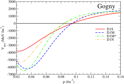
Figure 1: Dynamical potential as a function of the density for the D1S, D1M, D1M^∗ and D1N Gogny interactions.

As has been done in previous works Baym et al. (1971a, b); Xu et al. (2009a), the dynamical potential (34) can be approximated up to order $k^{2}$ by performing a Taylor expansion of the coefficients $D_{nn}$, $D_{pp}$ and $D_{np}=D_{pn}$ in Eqs. (LABEL:eq13). In this case the dynamical potential can be formally written as Pethick et al. (1995); Ducoin et al. (2007); Xu et al. (2009a)

$${\tilde{V}}_{\mathrm{dyn}}(\rho,k)=V_{\mathrm{ther}}(\rho)+\beta(\rho)k^{2}+\frac{4\pi e^{2}}{k^{2}+\frac{4\pi e^{2}}{\partial\mu_{e}/\partial\rho_{e}}},$$ (39)

where $V_{\mathrm{ther}}(\rho)$ has been defined in Eq. (37) and the expression of $\beta(\rho)$ is given in Eq. (68) of Appendix B. The practical advantage of Eq. (39) is that the $k$-dependence is separated from the $\rho$-dependence, whereas in the full expression for the dynamical potential in Eq. (36) they are not separated. It may be mentioned that in the case of Skyrme forces, which are zero-range interactions, the functions $D_{qq^{\prime}}(\rho,k)$ of Eqs. (LABEL:eq13) and (36) are quadratic functions of the momentum $k$ with constant coefficients.

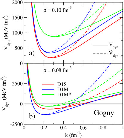
Figure 2: Momentum dependence of the dynamical potential at two different densities, $\rho=0.10$ fm^-3 (panel a) and $\rho=0.08$ fm^-3 (panel b), for the D1S, D1M and D1M^∗ Gogny interactions. The results plotted with solid lines are obtained using the full expression of the dynamical potential, given in Eq. (36), while the dashed lines are the results of its $k^{2}$-approximation, given in Eq. (39).

In order to examine the validity of the $k^{2}$-approximation (long-wavelength limit) of the dynamical potential, we plot in Fig. 2 the dynamical potential at a given density as a function of the momentum $k$ for both Eq. (36) (solid lines) and its $k^{2}$-approximation in Eq. (39) (dashed lines) for the Gogny forces D1S, D1M and D1M^∗. The momentum dependence of the dynamical potential at density $\rho=0.10$ fm^-3 is shown in the upper panel of Fig. 2. One sees that at this density the core has not reached the transition point for any of the considered Gogny forces, as the minima of the $V_{\mathrm{dyn}}(\rho,k)$ curves are positive. This implies that the system is stable against formation of clusters. In the lower panel of Fig. 2 the same results but at a density $\rho=0.08$ fm^-3 are shown. As the minimum of the dynamical potential for all forces is negative, the matter is unstable against cluster formation. From the results in Fig. 2 it can be seen that at low values of $k$ the agreement between the results of Eq. (36) and its approximation Eq. (39) is very good. However, at large momenta beyond $k$ of the minimum of the dynamical potential, there are increasingly larger differences between both calculations of the dynamical potential. This is consistent with the fact that Eq. (39) is the $k^{2}$-approximation of Eq. (36).

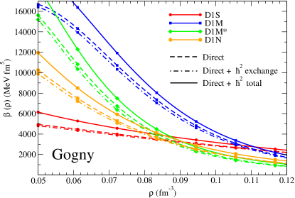
Figure 3: Coefficient $\beta(\rho)$ of Eq. (39) as a function of the density for a set of Gogny interactions. The dashed line includes only contributions coming from the direct energy, the dash-dotted lines include contributions coming from the direct energy and from the from the gradient effects of the exchange energy. Finally, the solid lines include all contributions to $\beta(\rho)$.

To investigate the impact of the direct and $\hbar^{2}$ contributions of the finite-range part of the interaction on the dynamical potential, in Fig. 3 we plot for Gogny forces the behaviour of the coefficient $\beta(\rho)$, which accounts for the finite-size effects in the stability condition of the core using the dynamical potential ${\tilde{V}}_{\mathrm{dyn}}(\rho,k)$. The dashed lines are the result for $\beta(\rho)$ when only the direct contribution from the finite range is taken into account. The dash-dotted lines give the value of $\beta(\rho)$ where, along with the direct contribution, the gradient effects from the exchange energy are included. Finally, solid lines correspond to the total value of $\beta(\rho)$, which includes the direct contribution and the complete $\hbar^{2}$ corrections, coming from both the exchange and kinetic energies. We see that for Gogny forces the gradient correction due to the $\hbar^{2}$ expansion of the exchange energy reduces the result of $\beta(\rho)$ from the direct contribution, at most, by 5%. When the gradient corrections from both the exchange and kinetic energies are taken together, the total result for $\beta(\rho)$ increases by 10% at most with respect to the direct contribution. The effects of the kinetic energy $\hbar^{2}$ corrections are around three times larger than the effects from the exchange energy $\hbar^{2}$ corrections and go in the opposite sense. Therefore, we conclude that the coefficient $\beta(\rho)$ is governed dominantly by the gradient expansion of the direct energy (see Appendix B), whereas the contributions from the $\hbar^{2}$ corrections to the exchange and kinetic energies are small corrections.

IV.2 The core-crust transition with finite-range effective interactions

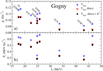
Figure 4: Transition density (panel a) and transition pressure (panel b) as a function of the slope of the symmetry energy calculated using the thermodynamical and the dynamical methods for a set of different Gogny interactions.

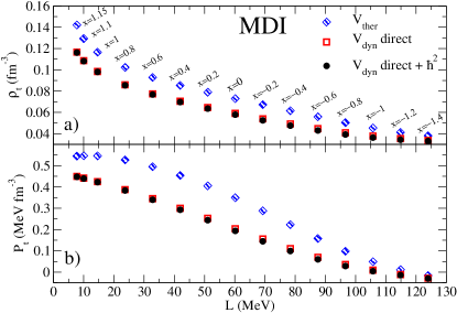
Figure 5: Same as Fig. 4 but for a family of MDI interactions.

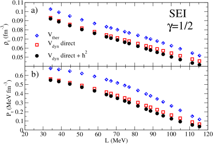
Figure 6: Same as Fig. 4 but for a family of SEI interactions of $\gamma=1/2$ ($K_{0}=237.5$ MeV).

Figure 7: Transition density as a function of the slope of the symmetry energy calculated using the dynamical method for a set of Skyrme, Gogny, MDI and SEI interactions.

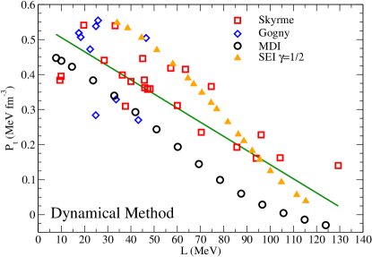
Figure 8: Transition density as a function of the slope of the symmetry energy calculated using the dynamical method for a set of Skyrme, Gogny, MDI and SEI interactions.

In Figs. 4, 5 and 6 we display, as a function of the slope of the symmetry energy $L$, the transition density (upper panels) and the transition pressure (lower panels) calculated with the thermodynamical ($V_{\mathrm{ther}}$) and the dynamical ($V_{\mathrm{dyn}}$) methods for three different types of finite-range interactions. The expression (36) with the complete momentum dependence of the dynamical potential has been used for the dynamical calculations. In the study of the transition properties we have employed several Gogny interactions Dechargé and Gogny (1980); Sellahewa and Rios (2014); Gonzalez-Boquera et al. (2017, 2018) (Fig. 4), a family of MDI forces Das et al. (2003); Xu and Ko (2010), with $L$ from $7.8$ to $124.0$ MeV (corresponding to values of the $x$ parameter ranging from $1.15$ to $-1.4$) (Fig. 5), and a family of SEI interactions Behera et al. (1998) with $\gamma=1/2$ and different values of the slope parameter $L$ (Fig. 6). Notice that the Gogny interactions have different nuclear matter saturation properties, whereas the parameterizations of the MDI or SEI families displayed in Figs. 5 and 6 have the same nuclear matter saturation properties within each family. In particular, all parametrizations of the MDI family considered here have the same nuclear matter incompressibility $K_{0}=212.6$ MeV, whereas the SEI parameterizations with $\gamma=1/2$ have $K_{0}=237.5$ MeV. Consistently with previous investigations (see e.g. Xu et al. (2009a); Xu and Ko (2010) and references therein) we find that for a given parameterization, the transition density obtained with the dynamical method is smaller than the prediction of the thermodynamical approach, as the surface and Coulomb contributions tend to further stabilize the uniform matter in the core against formation of clusters. The relative differences between the transition densities obtained with the thermodynamical and dynamical approaches are found to vary within the ranges $8-14\%$ for Gogny interactions, $15-30\%$ for MDI, and $10-25\%$ for SEI $\gamma=1/2$. For the MDI interactions, the trends are comparable to those found in Ref. Xu et al. (2009a) where the finite-size effects in the dynamical calculation were taken into account phenomenologically through assumed constant values for the $D_{nn}$, $D_{pp}$ and $D_{np}=D_{pn}$ coefficients. From the results of the transition pressure in Figs. 4–6, it is evident again that the thermodynamical method predicts larger values than its dynamical counterpart, which is also consistent with the findings in earlier works (Xu et al. (2009a); Xu and Ko (2010) and references therein). It is to be observed that we have performed the dynamical calculations of the transition properties in two different ways. On the one hand, we have considered the contributions to Eqs. (LABEL:eq13) from the direct energy only (the results are labelled as $V_{\mathrm{dyn}}$ direct in Figs. 4–6). Then, we have used the complete expression of Eqs. (LABEL:eq13) (the results are labelled as $V_{\mathrm{dyn}}$ direct$+\hbar^{2}$ in Figs. 4–6). As with our findings for the dynamical potential in the previous subsection, we see that for the three types of forces the finite-range effects on $\rho_{t}$ and $P_{t}$ coming from the $\hbar^{2}$ corrections of the exchange and kinetic energies are almost negligible compared to the effects due to the direct energy.

Figures 4–6 also provide information about the dependence of the transition properties with the slope of the symmetry energy. We can see that within the MDI and SEI families the transition density and pressure show a clear, nearly linear decreasing trend as a function of the slope parameter $L$. In contrast, the results of the several Gogny forces in Fig. 4 show a weak trend with $L$ for $\rho_{t}$ and almost no trend with $L$ for $P_{t}$. A more global analysis of the eventual dependence of the transition properties with the slope of the symmetry energy is displayed in Figs. 7 and 8. These figures include not only the results for the core-crust transition calculated using the considered sets of finite range interactions (Gogny, MDI and SEI of $\gamma=1/2$ interactions) but also the predictions of $23$ zero-range Skyrme forces covering the range of $L$ between 0 and 140 MeV. Using this large set of nuclear models of different nature, it can be seen that the decreasing trend of the transition density and pressure with rise in the slope $L$ of the symmetry energy is a general feature. However, the correlation of the transition properties with the slope parameter $L$ using all interactions is weaker than within a family of parametrizations where the saturation properties do not change. The correlation in the case of the transition density is found to be slightly better than in the case of the transition pressure. The reason for the weaker correlation obtained in the different Gogny sets (Fig. 4) and Skyrme sets (Figs. 7 and 8) is attributed to the fact that these sets have different nuclear matter saturation properties apart from the $L$ values.

Let us mention that we have also found that in the models used in this work the correlations between the transition density and pressure with the curvature of the symmetry energy, defined as

$$K_{\mathrm{sym}}=\left.9\rho_{\mathrm{sat}}^{2}\frac{\partial^{2}E_{\mathrm{sym}}(\rho)}{\partial\rho^{2}}\right|_{\rho_{\mathrm{sat}}},$$ (40)

are similar in quality to those found with the slope parameter $L$, in agreement with earlier literature Xu et al. (2009a); Carreau et al. .

Figure 9: Transition density (panel a) and transition pressure (panel b) as a function of the slope of the symmetry energy, calculated using the dynamical method for three SEI families with different nuclear matter incompressibilities.

In order to test the impact of the nuclear matter incompressibility on the correlations between the core-crust transition properties and the slope of the symmetry energy for a given type of finite-range interactions, we plot in Fig. 9 the transition density (panel a) and the transition pressure (panel b) against the $L$ parameter for SEI interactions of $\gamma=1/3$, $\gamma=1/2$ and $\gamma=1$, which correspond to nuclear matter incompressibilities $K_{0}$ of $220.0$ MeV, $237.5$ MeV and $282.3$ MeV, respectively, covering an extended range of $K_{0}$ values. From this figure we observe a high correlation with $L$ for the different sets of a given SEI force having the same incompressibility and differing only in the $L$ values. However, the comparison of the results obtained with the SEI forces of different incompressibility shows that higher transition density and pressure are predicted for the force sets with higher incompressibility. This also demonstrates, through the example of the nuclear matter incompressibility, a dependence of the features of the core-crust transition with the nuclear matter saturation properties of the force, on top of the dependence on the stiffness of the symmetry energy.

IV.3 Crustal properties of the neutron star

Figure 10: Neutron star crustal thickness (panels a), crustal mass (panels b) and crustal fraction of the moment of inertia (panels c) against the total mass of the neutron star for some Gogny (left), MDI (center) and SEI (right) interactions. The core-crust transition has been determined using the thermodynamical potential (dashed lines) and the dynamical potential using all direct and $\hbar^{2}$ contributions (solid lines).

Once we have obtained the location of the transition density and pressure, we can study how the differences between the results of the thermodynamical and dynamical methods affect the crustal properties of neutron stars, namely the crustal mass, crustal thickness and crustal fraction of the moment of inertia. For that purpose, we obtain the mass and radius of the NS core by solving the TOV equations from the center of the star to the transition point. We describe the core using the EOS of $\beta$-stable $npe\mu$ matter predicted by the finite-range forces. To obtain the properties of the NS crust, we use the method proposed by Zdunik, Fortin and Haensel Zdunik, J. L. et al. (2017), in which only the transition density and transition pressure are needed, but not the explicit knowledge of the EOS of the crust. In the work of Zdunik et al., the crustal thickness of a neutron star of mass $M$ is given by

$$R_{\mathrm{crust}}=\Phi R_{\mathrm{core}}\frac{1-2GM/R_{\mathrm{core}}c^{2}}{1-\Phi\left(1-2GM/R_{\mathrm{core}}c^{2}\right)},$$ (41)

with

$$\Phi\equiv\frac{(\alpha-1)R_{\mathrm{core}}c^{2}}{2GM}$$ (42)

and

$$\alpha=\left(\frac{\mu_{t}}{\mu_{0}}\right)^{2},$$ (43)

where $\mu_{t}=(P_{t}+{\cal H}_{t}c^{2})/\rho_{t}$ is the chemical potential at the core-crust transition, $\mu_{0}$ is the chemical potential at the surface of the neutron star and $R_{\mathrm{core}}$ is the thickness of the core. The crustal mass is obtained as

$$M_{\mathrm{crust}}=\frac{4\pi P_{t}R_{\mathrm{core}}^{4}}{GM_{\mathrm{core}}}\left(1-\frac{2GM_{\mathrm{core}}}{R_{\mathrm{core}}c^{2}}\right),$$ (44)

where $M_{\mathrm{core}}$ is the mass of the NS core. The total mass of the NS is $M=M_{\mathrm{crust}}+M_{\mathrm{core}}$. This approximate approach predicts the radius and mass of the crust with accuracy better than $\sim 1\%$ in $R_{\mathrm{crust}}$ and $\sim 5\%$ in $M_{\mathrm{crust}}$ for typical neutron star masses Zdunik, J. L. et al. (2017), while one circumvents the complex problem of computing the EOS of the crustal matter.

Finally, to compute the crustal fraction of the moment of inertia we use the approximation given by Lattimer and Prakash (2000, 2001, 2007), which allows one to express this quantity as

$$\frac{\Delta I_{\mathrm{crust}}}{I} = \frac{28\pi P_{t}R^{3}}{3Mc^{2}}\frac{\left(1-1.67\xi-0.6\xi^{2}\right)}{\xi}$$ (45)

$$\times\left[1+\frac{2P_{t}\left(1+5\xi-14\xi^{2}\right)}{\rho_{t}mc^{2}\xi^{2}}\right]^{-1},$$

where $\xi=\frac{GM}{Rc^{2}}$ is the compactness of the star, and $m$ is the baryon mass.

We plot in Fig. 10 the crustal thickness, crustal mass and crustal fraction of the moment of inertia against the total mass of the neutron star. As representative examples, we show the results provided by the D1M and D1M^∗ Gogny interactions, three MDI and three SEI forces with different $L$ values. All considered forces in this figure, except from the Gogny D1M and the MDI force with $L=42$ MeV, predict neutron stars of mass about $2M_{\odot}$, in agreement with astronomical observations Demorest et al. (2010); Antoniadis et al. (2013). For each interaction we have obtained the crustal properties using the transition point given by the thermodynamical and the dynamical approaches. In general, the global behaviour of these properties is similar for all three types of finite-range forces. This is true for both the methods of calculations, where the thermodynamical model gives higher values than its dynamical counterpart. The influence of the transition point is smaller on the crustal radius, and has a larger impact in the calculation of the crustal mass and crustal fraction of the moment of inertia. The differences between the predictions using the core-crust transition found with the thermodynamical or with the dynamical methods are larger for interactions with a larger value of $L$. These differences are very prominent in the typical NS mass region and could influence the properties where the crust has an important role, such as pulsar glitches Link et al. (1999); Fattoyev and Piekarewicz (2010); Chamel (2013); Piekarewicz et al. (2014); Newton et al. (2015); Gonzalez-Boquera et al. (2017).

V Summary and Conclusions

In this work we have analyzed the core-crust transition in neutron stars estimated with the dynamical method using several finite-range interactions of Gogny, MDI and SEI types. This study enlarges previous studies available in the literature, which were basically performed, to our knowledge, in the case of the MDI forces. We follow closely the original method developed by Baym, Bethe and Pethick to derive the energy curvature matrix in momentum space. The contribution coming from the direct energy is obtained through the expansion of its finite-range form factors in terms of distributions, which allows one to write the direct contribution beyond the so-called long-wavelength limit (expansion till $k^{2}$-order). Moreover, the Extended Thomas-Fermi expansion of the density matrix is used to write the kinetic and exchange energies as the sum of a bulk term plus a $\hbar^{2}$ correction. This $\hbar^{2}$ term can be written as a linear combination of the square of the gradients of the neutron and proton distributions, with density-dependent coefficients, which in turn provide a $k^{2}$-dependence in the energy curvature matrix.

We find that the effects of the finite-range part of the nuclear interaction on the energy curvature matrix mainly arises from the direct part of the energy, where the $\hbar^{2}$ contributions from kinetic and exchange part of finite range interaction can be considered as small correction.

We have analyzed the global behaviour of the core-crust transition density and pressure as a function of the slope of the symmetry energy at saturation for a large set of non-relativistic nuclear models, which include finite-range interactions as well as Skyrme forces. The results for MDI sets found under the present formulation are in good agreement with the earlier ones reported by Xu and Ko, where they use a different density matrix expansion to deal with the exchange energy and adopted the Vlasov equation method to obtain the curvature energy matrix. We also observe that within the MDI and SEI families of interactions, the transition density and pressure are highly correlated with the slope of the symmetry energy at saturation. However, when nuclear models with different saturation properties are considered, these correlations are deteriorated, in particular the one related to the transition pressure.

Finally, we have studied the crustal properties of neutron stars, such as the crustal thickness, crustal mass and crustal fraction of moment of inertia, by solving the TOV equations from the center to the point corresponding to the transition density obtained from the dynamical as well as in the thermodynamical approach. It is found that the transition point determined with the thermodynamical and dynamical methods has a relevant impact on the considered crustal properties, in particular for models with stiff symmetry energy. These crustal properties play a crucial role in the prediction of several observed phenomena, like glitches, r-mode oscillation, etc. Therefore, the core-crust transition density needs to be ascertained as precisely as possible by taking into account the associated physical conditions in order to have a realistic estimation of the observed phenomena.

Appendix A

The ETF approximation to the HF energy for non-local potentials consists of replacing the quantal density matrix by the semiclassical one that contains, in addition to the bulk (Slater) term, corrective terms depending on the second-order derivatives of the proton and neutron densities, which account for contributions up to $\hbar^{2}$-order. The angle-averaged semiclassical ETF density matrix, derived in Refs. Centelles et al. (1998); Gridnev et al. (1998); Soubbotin and Viñas (2000), for each kind of nucleon reads

$${\tilde{\rho}}({\bf R},s) = =\rho_{0}({\bf R},s)+\rho_{2}({\bf R},s)=\frac{3j_{1}(k_{F}s)}{k_{f}s}\rho+\frac{s^{2}}{216}\left\{\left[\left(9-2k_{F}\frac{f_{k}}{f}-2k_{F}^{2}\frac{f_{kk}}{f}+k_{F}^{2}\frac{f_{k}^{2}}{f}\right)\frac{j_{1}(k_{F}s)}{k_{F}s}-4j_{0}(k_{F}s)\right]\frac{({\bf\nabla}\rho)^{2}}{\rho}\right.$$

$$- \left.\left[\left(18+6k_{F}\frac{f_{k}}{f}\right)\frac{j_{1}(k_{F}s)}{k_{F}s}-3j_{0}(k_{F}s)\right]\Delta\rho-\left[18\rho\frac{\Delta f}{f}+\left(18-6k_{F}\frac{f_{k}}{f}\right)\frac{{\bf\nabla}\rho\cdot{\bf\nabla}f}{f}\right.\right.$$

$$+ \left.\left.12k_{F}\frac{{\bf\nabla}\rho\cdot{\bf\nabla}f_{k}}{f}-9\rho\frac{({\bf\nabla}f)^{2}}{f}\right]\frac{j_{1}(k_{F}s)}{k_{F}s}\right\},$$

where $\rho({\bf R})$ is the local density, $k_{F}=(3\pi^{2}\rho({\bf R}))^{1/3}$ is the corresponding Fermi momentum for each type of nucleon, and $j_{1}(k_{F}s)$ is the $l=1$ spherical Bessel function. In Eq. (LABEL:eqA1) $f=\left.f({\bf R},k)\right|_{k=k_{F}}$ is the inverse of the position and momentum dependent effective mass, defined for each type of nucleon as

$$f({\bf R},k)=\frac{m}{m^{*}({\bf R},k)}=1+\frac{m}{\hbar^{2}k}\frac{\partial V^{F}_{0}({\bf R},k)}{\partial k}.$$ (47)

computed at the $k=k_{F}$ (see below), and $f_{k}=\left.f_{k}({\bf R},k)\right|_{k=k_{F}}$ and $f_{kk}=\left.f_{kk}({\bf R},k)\right|_{k=k_{F}}$ are its first and second derivatives with respect to $k$. In Eq. (47), $V^{F}_{0}({\bf R},k)$ is the Wigner transform of the exchange potential (7) given by

$$V^{F}_{0}({\bf R},k)=\int d{\bf s}V^{F}_{0}({\bf R},s)e^{-i{\bf k}\cdot{\bf s}}=\int d{\bf s}V_{0}^{F}({\bf R},s)j_{0}(k,s),$$ (48)

which leads to Eq. (12) of the main text. Notice that due to the structure of the exchange potential (12), the space dependence of the effective mass for each kind of nucleon is through the Fermi momenta of both type of nucleon, neutrons and protons, i.e. $f_{q}=f_{q}(k,k_{Fn}({\bf R}),k_{Fp}({\bf R}))$ ($q=n,p$). When the inverse effective mass and its derivatives with respect to $k$ are used in (LABEL:eqA1), an additional space dependence arises from the replacement of the momentum $k$ by the local Fermi momentum $k_{F}({\bf R})$.

Using the DM (LABEL:eqA1) the explicit form of the semiclassical kinetic energy at the ETF level for either neutrons or protons can be written as:

$$\tau_{ETF}({\bf R}) = \left.\left(\frac{1}{4}\Delta_{R}-\Delta_{s}\right){\tilde{\rho}}({\bf R},s)\right|_{s=0}=\tau_{0}+\tau_{2},$$ (49)

which consists of the well-known TF term

$$\tau_{0}=\frac{3}{5}k_{F}^{2}\rho,$$ (50)

plus the $\hbar^{2}$ contribution

$$\tau_{2}({\bf R}) = \frac{1}{36}\frac{({\bf\nabla}\rho)^{2}}{\rho}\left[1+\frac{2}{3}k_{F}\frac{f_{k}}{f}+\frac{2}{3}k_{F}^{2}\frac{f_{kk}}{f}-\frac{1}{3}k_{F}^{2}\frac{f_{k}^{2}}{f^{2}}\right]+\frac{1}{12}\Delta\rho\left[4+\frac{2}{3}k_{F}\frac{f_{k}}{f}\right]$$ (51)

$$+ \frac{1}{6}\rho\frac{\Delta f}{f}+\frac{1}{6}\frac{{\bf\nabla}\rho\cdot{\bf\nabla}f}{f}\left[1-\frac{1}{3}k_{F}\frac{f_{k}}{f}\right]+\frac{1}{9}\frac{{\bf\nabla}\rho\cdot{\bf\nabla}f_{k}}{f}-\frac{1}{12}\rho\frac{({\bf\nabla}f)^{2}}{f^{2}}.$$

This $\hbar^{2}$ contribution reduces to the standard $\hbar^{2}$ expression for local forces Brack et al. (1985) if the effective mass depends only on the position and not on the momentum.

The direct energy is easily obtained using the diagonal part of the DM, which at ETF level reduces to the local density $\rho$. The exchange energy density, which is local within the ETF approximation, is obtained from the exchange potential (48) and is given by

$${\cal H}_{exch}({\bf R})=\frac{1}{2}\int d{\bf s}\rho_{0}({\bf R},s)V_{0}^{F}({\bf R},s)+\int d{\bf s}\rho_{2}({\bf R},s)V^{F}_{0}({\bf R},s),$$ (52)

from where, and after some algebra explained in detail in Ref. Soubbotin and Viñas (2000), one can recast the $\hbar^{2}$ contribution to the exchange energy for each kind of nucleon as

$${\cal H}_{exch,2}({\bf R})=\frac{\hbar^{2}}{2M}\left[(f-1)\left(\tau_{ETF}-\frac{3}{5}k_{F}^{2}\rho-\frac{1}{4}\Delta\rho\right)+k_{F}f_{k}\left(\frac{1}{27}\frac{({\bf\nabla}\rho)^{2}}{\rho}-\frac{1}{36}\Delta\rho\right)\right].$$ (53)

Notice that $\tau_{ETF}-\frac{3}{5}k_{F}^{2}\rho=\tau_{2}$ and that $\Delta\rho$ vanishes under integral sign if spherical symmetry in coordinate space is assumed. Therefore the sum of the total kinetic energy and the $\hbar^{2}$ contribution to exchange energy can be written as the pure TF kinetic part, which contributes to the bulk energy, plus an additional $\hbar^{2}$ term, which depends on the local Fermi momentum $k_{F}$ and on second-order derivatives of the nuclear density:

$$\int d{\bf R}\left[{\cal H}_{kin}({\bf R})+{\cal H}_{exch,2}({\bf R})\right]=\frac{\hbar^{2}}{2M}\int d{\bf R}\left\{\tau_{0}+\left[f\tau_{2}-\frac{1}{4}f\Delta\rho+k_{F}f_{k}\left(\frac{1}{27}\frac{({\bf\nabla}\rho)^{2}}{\rho}-\frac{1}{36}\Delta\rho\right)\right]\right\}.$$ (54)

By performing a suitable partial integration of the Laplacian of the density in Eqs. (51) and (54), one can recast the $\hbar^{2}$ contribution to (54) as a function of the density multiplied by the square gradient of the density as we have pointed out in the main text (see Eq. (13)).

The full $\hbar^{2}$ contribution to the total energy corresponding to the finite-range central interaction (2), given by Eq. (54) for each kind of nucleon, can be written, after partial integration, as:

$$E_{\hbar^{2}}=\int d{\bf R}\bigg{[}B_{nn}(\rho_{n},\rho_{p})\big{(}{\bf\nabla}\rho_{n}\big{)}^{2}+B_{pp}(\rho_{n},\rho_{p})\big{(}{\bf\nabla}\rho_{p}\big{)}^{2}+2B_{np}(\rho_{n},\rho_{p}){\bf\nabla}\rho_{n}\cdot{\bf\nabla}\rho_{p}\bigg{]},$$ (55)

where the like coefficients of the gradients of the densities are

$$B_{nn}(\rho_{n},\rho_{p}) = \frac{\hbar^{2}}{2M}\frac{1}{108}\left\{\left[3f_{n}+k_{Fn}(2f_{nk}-3f_{nk_{Fn}})+k^{2}_{Fn}(5f_{nkk}+3f_{nkk_{Fn}})\right.\right.$$ (56)

$$- \left.\left.k^{2}_{Fn}\frac{(2f_{nk}+f_{nk_{Fn}})^{2}}{f_{n}}\right]\frac{1}{\rho_{n}}-\frac{\rho_{p}}{\rho_{n}^{2}}k^{2}_{Fn}\frac{f^{2}_{pk_{Fn}}}{f_{p}}\right\}$$

and a similar expression for $B_{pp}(\rho_{n},\rho_{p})$ obtained by exchanging $n$ by $p$ in Eq. (56). The unlike coefficient $B_{np}(\rho_{n},\rho_{p})$ of Eq. (55) reads:

$$B_{np}(\rho_{n},\rho_{p}) = B_{pn}(\rho_{p},\rho_{n})=-\frac{\hbar^{2}}{2M}\frac{1}{316}\left\{\left[3k_{Fp}f_{nk_{Fp}}-3k_{Fn}k_{Fp}f_{nkk_{Fp}}+\frac{2k_{Fn}k_{Fp}(2f_{nk}+f_{nk_{Fn}})f_{nk_{Fp}}}{f_{n}}\right]\frac{1}{\rho_{p}}\right.$$ (57)

$$+ \left.\left[3k_{Fn}f_{pk_{Fn}}-3k_{Fp}k_{Fn}f_{pkk_{Fn}}+\frac{2k_{Fp}k_{Fn}(2f_{pk}+f_{pk_{Fp}})f_{pk_{Fn}}}{f_{p}}\right]\frac{1}{\rho_{n}}\right\}.$$

As mentioned before, all derivatives of the neutron (proton) inverse effective mass $f_{q}(k,k_{Fq},k_{Fq^{\prime}})$ with respect to the momentum $k$, $f_{qk}(k_{Fq},k_{Fq^{\prime}})$, are evaluated at the neutron (proton) Fermi momentum $k_{Fq}$, i.e. $f_{qk}(k_{Fq},k_{Fq^{\prime}})=\left.\frac{\partial f_{q}(k,k_{Fq},k_{Fq^{\prime}})}{\partial k}\right|_{k=k_{Fq}}$, $f_{qkk}(k_{Fq},k_{Fq^{\prime}})=\left.\frac{\partial^{2}f_{q}(k,k_{Fq},k_{Fq^{\prime}})}{\partial k^{2}}\right|_{k=k_{Fq}}$, $f_{qkk_{Fq^{\prime}}}(k_{Fq},k_{Fq^{\prime}})=\left.\frac{\partial^{2}f_{q}(k,k_{Fq},k_{Fq^{\prime}})}{\partial k\partial k_{Fq^{\prime}}}\right|_{k=k_{Fq}}$, etc.

Appendix B

In this Appendix we derive the direct term in Eq. (21) due to the fluctuating density. Let us first obtain the gradient expansion of the direct energy coming from the finite-range part of the force. For the sake of simplicity we consider a single Wigner term. The result for the case including spin and isospin exchange operators can be obtained analogously. In the case of a Wigner term we have

$$E_{dir}=\frac{1}{2}\int d{\bf R}d{\bf s}\rho({\bf R})\rho({\bf R}-{\bf s})v({\bf s}).$$ (58)

Following the procedure of Ref. Durand et al. (1993), a central finite-range interaction can be expanded in a series of distributions as follows:

$$v({s})=\sum_{n=0}^{\infty}c_{2n}\nabla^{2n}\delta({\bf s}),$$ (59)

where the coefficients $c_{2n}$ are chosen in such a way that the expansion (59) gives the same moments of the interaction $v$($s$). This implies that Durand et al. (1993)

$$c_{2n}=\frac{1}{(2n+1)!}\int d{\bf s}s^{2n}v({s}),$$ (60)

which allows one to determine the values of the coefficients $c_{2n}$ for any value of $n$. Using this expansion, the direct energy (58) can be written as

$$E_{dir}=\sum_{n=0}^{\infty}\frac{c_{2n}}{2}\int d{\bf R}d{\bf s}\rho({\bf R})\rho({\bf R}-{\bf s})\nabla^{2n}\delta({\bf s})=\sum_{n=0}^{\infty}\frac{c_{2n}}{2}\int d{\bf R}\rho({\bf R})\nabla^{2n}\rho({\bf R}).$$ (61)

Expanding now the density $\rho({\bf R})$ in its uniform and varying contributions, the direct energy due to the fluctuating part of the density becomes:

$$\delta E_{dir}=\sum_{n=0}^{\infty}\frac{c_{2n}}{2}\int d{\bf R}\delta\rho({\bf R})\nabla^{2n}\delta\rho({\bf R}).$$ (62)

Notice that the splitting of the density (14) also provides a contribution to the non-fluctuating energy $E_{0}({\rho_{0}})$ through the constant density $\rho_{0}$. Linear terms in $\delta\rho({\bf R})$ do not contribute to the direct energy by the reasons discussed in the main text (Section III). Proceeding as in the main text to transform integrals in coordinate space into integrals in momentum space (see Eqs. (19) and (20)) after some algebra the fluctuating correction to the direct energy can be written as follows:

$$\delta E_{dir}=\frac{1}{2}\int\frac{d{\bf k}}{(2\pi)^{3}}\delta n({\bf k})\delta n^{*}({\bf k}){\cal F}(k),$$ (63)

where

$${\cal F}(k)=\sum_{n=0}^{\infty}c_{2n}k^{2n}$$ (64)

is a series encoding the response of the direct energy to the perturbation induced by the varying density. This series is the Taylor expansion of the Fourier transform of the form factor $v(s)$. In the case of Gaussian ($e^{-s^{2}/\alpha^{2}}$) or Yukawian ($e^{-\mu s}/\mu s$) form factors one obtains, respectively,

$${\cal F}(k)=\pi^{3/2}\alpha^{3}e^{-\alpha^{2}k^{2}/4}$$ (65)

and

$${\cal F}(k)=\frac{4\pi}{\mu(\mu^{2}+k^{2})}.$$ (66)

Note that if in (66) one takes $\mu$=0, one recovers the result of the direct Coulomb potential Baym et al. (1971b).

For the nuclear direct potential the first term ($c_{0}$) of the series for ${\cal F}(k)$, which can be written as ${\cal F}(0)$, corresponds to the bulk contribution associated to the fluctuating density $\delta\rho({\bf R})$, i.e. it also contributes to $\mu_{n}$ and $\mu_{p}$ in Eq. (21). Then, the fluctuating correction to the direct energy in Eq. (21) is given by

$$\delta E_{dir} = \frac{1}{2}\int\frac{d{\bf k}}{(2\pi)^{3}}\sum_{m}\left[D_{L,dir}^{m}\left(\delta n_{n}({\bf k})\delta n^{*}_{n}({\bf k})+\delta n_{p}({\bf k})\delta n^{*}_{p}({\bf k})\right)\right.$$ (67)

$$+ \left.D_{U,dir}^{m}\left(\delta n_{n}({\bf k})\delta n^{*}_{p}({\bf k})+\delta n_{p}({\bf k})\delta n^{*}_{n}({\bf k})\right)\right]({\cal F}_{m}(k)-{\cal F}_{m}(0))$$

Let us also point out that if the series ${\cal F}(k)$ is cut at first order, i.e. taking only the $n=1$ term of the series, $c_{2}$, one recovers the typical $k^{2}$ dependence corresponding to square gradient terms in the energy density functional. If this expansion up to quadratic terms in $k$ is used, the dynamical potential potential can be written as Eq. (39), where the coefficient $\beta(\rho)$ reads

$$\beta(\rho)=\left[\sum_{m}D^{m}_{L,dir}c^{m}_{2}+2B_{pp}\left(\rho_{n},\rho_{p}\right)\right]+\frac{\left(\frac{\partial\mu_{p}}{\partial\rho_{n}}\right)^{2}}{\left(\frac{\partial\mu_{n}}{\partial\rho_{n}}\right)^{2}}\left[\sum_{m}D^{m}_{L,dir}c^{m}_{2}+2B_{nn}\left(\rho_{n},\rho_{p}\right)\right]-2\frac{\frac{\partial\mu_{p}}{\partial\rho_{n}}}{\frac{\partial\mu_{n}}{\partial\rho_{n}}}\left[\sum_{m}D^{m}_{U,dir}c^{m}_{2}+2B_{np}\left(\rho_{n},\rho_{p}\right)\right],$$ (68)

and the $B_{qq}\left(\rho_{n},\rho_{p}\right)$ and $B_{qq^{\prime}}\left(\rho_{n},\rho_{p}\right)$ functions have been given in Eqs. (56) and (57), corresponding to the $\hbar^{2}$ contributions coming from the expansion of the energy density functional. Moreover, for Gaussian form factors one has

$$c_{2}^{m}=-\frac{\pi^{3/2}\alpha_{m}^{5}}{4},$$ (69)

whereas for Yukawian form factors one has

$$c_{2}^{m}=-\frac{4\pi}{\mu_{m}^{5}}.$$ (70)

References

- Shapiro and Teukolsky (1983) S. L. Shapiro and S. A. Teukolsky, Black holes, white dwarfs, and neutron stars: The physics of compact objects, Vol. 20 (John Wiley & Sons, 1983) p. 663.
- Haensel et al. (2007) P. Haensel, A. Y. Potekhin, and D. G. Yakovlev, Neutron Stars 1: Equation of State and Structure (Springer, 2007).
- Rüster et al. (2006) S. B. Rüster, M. Hempel, and J. Schaffner-Bielich, Phys. Rev. C 73, 035804 (2006).
- Hempel and Schaffner-Bielich (2007) M. Hempel and J. Schaffner-Bielich, Journal of Physics G: Nuclear and Particle Physics 35, 014043 (2007).
- Baym et al. (1971a) G. Baym, C. Pethick, and P. Sutherland, Astrophys. J. 170, 299 (1971a).
- Kubis (2007) S. Kubis, Phys. Rev. C 76, 025801 (2007).
- Ducoin et al. (2007) C. Ducoin, P. Chomaz, and F. Gulminelli, Nucl. Phys. A 789, 403 (2007).
- Xu et al. (2009a) J. Xu, L.-W. Chen, B.-A. Li, and H.-R. Ma, Astrophys. J. 697, 1549 (2009a).
- Xu et al. (2009b) J. Xu, L.-W. Chen, B.-A. Li, and H.-R. Ma, Phys. Rev. C 79, 035802 (2009b).
- Xu et al. (2010) J. Xu, L.-W. Chen, C. M. Ko, and B.-A. Li, Phys. Rev. C 81, 055805 (2010).
- Xu and Ko (2010) J. Xu and C. M. Ko, Phys. Rev. C 82, 044311 (2010).
- Moustakidis et al. (2010) C. C. Moustakidis, T. Nikšić, G. A. Lalazissis, D. Vretenar, and P. Ring, Phys. Rev. C 81, 065803 (2010).
- Moustakidis (2012) C. C. Moustakidis, Phys. Rev. C 86, 015801 (2012).
- Seif and Basu (2014) W. M. Seif and D. N. Basu, Phys. Rev. C 89, 028801 (2014).
- Routray et al. (2016) T. R. Routray, X. Viñas, D. N. Basu, S. P. Pattnaik, M. Centelles, L. B. Robledo, and B. Behera, J. Phys. G Nucl. Part. Phys. 43, 105101 (2016).
- Gonzalez-Boquera et al. (2017) C. Gonzalez-Boquera, M. Centelles, X. Viñas, and A. Rios, Phys. Rev. C 96, 065806 (2017).
- Baym et al. (1971b) G. Baym, H. A. Bethe, and C. J. Pethick, Nucl. Phys. A 175, 225 (1971b).
- Lattimer and Swesty (1991) J. M. Lattimer and F. D. Swesty, Nuclear Physics A 535, 331 (1991).
- Shen et al. (1998a) H. Shen, H. Toki, K. Oyamatsu, and K. Sumiyoshi, Nuclear Physics A 637, 435 (1998a).
- Shen et al. (1998b) H. Shen, H. Toki, K. Oyamatsu, and K. Sumiyoshi, Progress of Theoretical Physics 100, 1013 (1998b).
- Douchin and Haensel (2001) F. Douchin and P. Haensel, Astron. Astrophys. 380, 151 (2001).
- Sharma et al. (2015) B. K. Sharma, M. Centelles, X. Viñas, M. Baldo, and G. F. Burgio, Astron. Astrophys. 584, A103 (2015).
- (23) T. Carreau, F. Gulminelli, and J. Margueron, arXiv:1902.07032 (2019) .
- Pethick et al. (1995) C. Pethick, D. Ravenhall, and C. Lorenz, Nucl. Phys. A 584, 675 (1995).
- Horowitz and Piekarewicz (2001a) C. J. Horowitz and J. Piekarewicz, Phys. Rev. Lett. 86, 5647 (2001a).
- Horowitz and Piekarewicz (2001b) C. J. Horowitz and J. Piekarewicz, Phys. Rev. C 64, 062802 (2001b).
- Carriere et al. (2003) J. Carriere, C. J. Horowitz, and J. Piekarewicz, Astrophys. J. 593, 463 (2003).
- Chomaz et al. (2004) P. Chomaz, M. Colonna, and J. Randrup, Phys. Rep. 389, 263 (2004).
- Providência et al. (2006) C. Providência, L. Brito, S. S. Avancini, D. P. Menezes, and P. Chomaz, Phys. Rev. C 73, 025805 (2006).
- Ducoin et al. (2008a) C. Ducoin, J. Margueron, and P. Chomaz, Nucl. Phys. A 809, 30 (2008a).
- Ducoin et al. (2008b) C. Ducoin, C. Providência, A. M. Santos, L. Brito, and P. Chomaz, Phys. Rev. C 78, 055801 (2008b).
- Pais et al. (2010) H. Pais, A. Santos, L. Brito, and C. Providência, Phys. Rev. C 82, 025801 (2010).
- Oyamatsu and Iida (2007) K. Oyamatsu and K. Iida, Phys. Rev. C 75, 015801 (2007).
- Negele and Vautherin (1972) J. W. Negele and D. Vautherin, Phys. Rev. C 5, 1472 (1972).
- Negele and Vautherin (1975) J. W. Negele and D. Vautherin, Phys. Rev. C 11, 1031 (1975).
- Dechargé and Gogny (1980) J. Dechargé and D. Gogny, Phys. Rev. C 21, 1568 (1980).
- Berger et al. (1991) J. F. Berger, M. Girod, and D. Gogny, Comp. Phys. Comm. 63, 365 (1991).
- Chappert et al. (2008) F. Chappert, M. Girod, and S. Hilaire, Phys. Lett. B 668, 420 (2008).
- Goriely et al. (2009) S. Goriely, S. Hilaire, M. Girod, and S. Péru, Phys. Rev. Lett. 102, 242501 (2009).
- Sellahewa and Rios (2014) R. Sellahewa and A. Rios, Phys. Rev. C 90, 054327 (2014).
- Friedman and Pandharipande (1981) B. Friedman and V. Pandharipande, Nucl. Phys. A 361, 502 (1981).
- Gonzalez-Boquera et al. (2018) C. Gonzalez-Boquera, M. Centelles, X. Viñas, and L. Robledo, Physics Letters B 779, 195 (2018).
- Demorest et al. (2010) P. B. Demorest, T. Pennucci, S. M. Ransom, M. S. E. Roberts, and J. W. T. Hessels, Nature 467, 1081 (2010).
- Antoniadis et al. (2013) J. Antoniadis, P. C. C. Freire, N. Wex, T. M. Tauris, R. S. Lynch, M. H. van Kerkwijk, M. Kramer, C. Bassa, V. S. Dhillon, T. Driebe, J. W. T. Hessels, V. M. Kaspi, V. I. Kondratiev, N. Langer, T. R. Marsh, M. a. McLaughlin, T. T. Pennucci, S. M. Ransom, I. H. Stairs, J. van Leeuwen, J. P. W. Verbiest, and D. G. Whelan, Science 340, 448 (2013).
- Das et al. (2003) C. B. Das, S. Das Gupta, C. Gale, and B.-A. Li, Phys. Rev. C 67, 034611 (2003).
- Behera et al. (1998) B. Behera, T. R. Routray, and R. K. Satpathy, Journal of Physics G: Nuclear and Particle Physics 24, 2073 (1998).
- Behera et al. (2005) B. Behera, T. Routray, A. Pradhan, S. Patra, and P. Sahu, Nuclear Physics A 753, 367 (2005).
- Behera et al. (2013) B. Behera, X. Viñas, M. Bhuyan, T. R. Routray, B. K. Sharma, and S. K. Patra, Journal of Physics G: Nuclear and Particle Physics 40, 095105 (2013).
- Behera et al. (2015) B. Behera, X. Viñas, T. R. Routray, and M. Centelles, Journal of Physics G: Nuclear and Particle Physics 42, 045103 (2015).
- Soubbotin and Viñas (2000) V. Soubbotin and X. Viñas, Nuclear Physics A 665, 291 (2000).
- Soubbotin et al. (2003) V. B. Soubbotin, V. I. Tselyaev, and X. Viñas, Phys. Rev. C 67, 014324 (2003).
- Krewald et al. (2006) S. Krewald, V. B. Soubbotin, V. I. Tselyaev, and X. Viñas, Phys. Rev. C 74, 064310 (2006).
- Behera et al. (2016) B. Behera, X. Viñas, T. R. Routray, L. M. Robledo, M. Centelles, and S. P. Pattnaik, Journal of Physics G: Nuclear and Particle Physics 43, 045115 (2016).
- Nakada (2003) H. Nakada, Phys. Rev. C 68, 014316 (2003).
- Robledo (2002) L. Robledo, HFBaxial computer code (2002).
- Campi and Bouyssy (1978) X. Campi and A. Bouyssy, Physics Letters B 73, 263 (1978).
- Bouyssy and Campi (1979) A. Bouyssy and X. Campi, Nukleonika 24, 1 (1979).
- Gridnev et al. (1998) K. Gridnev, V. Soubbotin, X. Viñas, and M. Centelles, Quantum Theory in honour of Vladimir A. Fock, Y. Novozhilov and V. Novozhilov (Publishing Group of St.Petersburg University, 1998) p. 118 arXiv 1704.03858.
- Zdunik, J. L. et al. (2017) Zdunik, J. L., Fortin, M., and Haensel, P., A&A 599, A119 (2017).
- Lattimer and Prakash (2000) J. M. Lattimer and M. Prakash, Phys. Rep. 333-334, 121 (2000).
- Lattimer and Prakash (2001) J. M. Lattimer and M. Prakash, The Astrophysical Journal 550, 426 (2001).
- Lattimer and Prakash (2007) J. M. Lattimer and M. Prakash, Phys. Rep. 442, 109 (2007), the Hans Bethe Centennial Volume 1906-2006.
- Link et al. (1999) B. Link, R. I. Epstein, and J. M. Lattimer, Phys. Rev. Lett. 83, 3362 (1999).
- Fattoyev and Piekarewicz (2010) F. J. Fattoyev and J. Piekarewicz, Phys. Rev. C 82, 025810 (2010), arXiv:1006.3758 [nucl-th] .
- Chamel (2013) N. Chamel, Phys. Rev. Lett. 110, 011101 (2013).
- Piekarewicz et al. (2014) J. Piekarewicz, F. J. Fattoyev, and C. J. Horowitz, Phys. Rev. C 90, 015803 (2014).
- Newton et al. (2015) W. G. Newton, S. Berger, and B. Haskell, Mon. Not. R. Astron. Soc. 454, 4400 (2015), arXiv:1506.01445 .
- Centelles et al. (1998) M. Centelles, X. Viñas, M. Durand, P. Schuck, and D. Von-Eiff, Annals of Physics 266, 207 (1998).
- Brack et al. (1985) M. Brack, C. Guet, and H.-B. Håkansson, Phys. Rep. 123, 275 (1985).
- Durand et al. (1993) M. Durand, P. Schuck, and X. Viñas, Z. Physik A - Hadrons and Nuclei 346, 87 (1993).