Tracking the footprints of the radio pulsar B1727$-$47: proper motion, host supernova remnant, and the glitches

Abstract

The bright radio pulsar B1727$-$47 with a characteristic age of $80$ kyr is among the first pulsars discovered 50 yr ago. Using its regular timing observations and interferometric positions at three epochs, we measured, for the first time, the pulsar proper motion of $151\pm 19$ mas yr^-1. At the dispersion measure distance of $\gtrsim 2.7$ kpc, this would suggest a record transverse velocity of the pulsar $\gtrsim 1900$ km s^-1. However, a backward extrapolation of the pulsar track to its birth epoch points remarkably close to the center of the evolved nearby supernova remnant RCW 114, which suggests genuine association of the two objects. In this case, the pulsar is substantially closer ($\sim 0.6$ kpc) and younger ($\sim 50$ kyr), and its velocity ($\sim 400$ km s^-1) is compatible with the observed pulsar velocity distribution. We also identified two new glitches of the pulsar. We discuss implications of our results on the pulsar and remnant properties.

1 Introduction

Associations of pulsars (PSRs) with their supernova remnants (SNRs) provide crucial information on the properties of these astrophysical objects born at the same supernova explosions. In particular, this allows one to get the most reliable constraints on objects’ ages, local environments, and on supernova progenitor parameters. Justified associations are useful for the study of the whole PSR–SNR population which is important for unveiling the routes of the final stages of the stellar evolution (e.g., Heger et al., 2003).

Relatively short lifetimes of the extended remnants ($\lesssim 100$ kyr) limit the identification of each pulsar with its SNR. So far only about fifteen radio PSRs have been firmly identified with SNRs (e.g., Yao et al., 2017). The number of candidate associations is permanently growing due to ongoing progress in the observational instrumentation. However, a significant amount of them could be due to a chance spatial coincidence (Gaensler & Johnston, 1995). Therefore, each possible PSR–SNR connection requires several independent justifications. Among them, the highest priority is granted to PSR proper motion (p.m.) measurements (e.g., Kaspi, 1996). Generally, a pulsar must be kicked from its parent supernova explosion center. If the p.m. track of the pulsar misses the remnant center by a significant distance, this can be considered as a strong argument against the association (e.g., Brisken et al., 2006), although sometimes the off-centric asymmetric solutions are possible (e.g., Gvaramadze, 2002).

Table 1: Published B1727 coordinates

Epoch	R.A., B1950	Decl., B1950	R.A., J2000	Decl., J2000	Telescope,
MJD, yr month					Reference
41638, 1972 Nov	17h27m56s(1)	$-$47∘42′22′′(2)	17h31m42$.\!\!^{\rm s}$6(1.0)	$-$47∘44′33$.\!\!^{\prime\prime}$7(2.0)	Molonglo, 1
43494, 1977 Dec	17h27m55$.\!\!^{\rm s}$38(2)	$-$47∘42′21$.\!\!^{\prime\prime}$4(5)	17h31m41$.\!\!^{\rm s}$99(2)	$-$47∘44′33$.\!\!^{\prime\prime}$0(5)	Tidbinbilla, 2
47780.5, 1989 Sep	17h27m55$.\!\!^{\rm s}$42(6)	$-$47∘42′23′′(1)	17h31m42$.\!\!^{\rm s}$06(6)	$-$47∘44′34$.\!\!^{\prime\prime}$7(1.0)	Mt Pleasant, 3
50059, 1995 Dec			17h31m42$.\!\!^{\rm s}$103(5)	$-$47∘44′34$.\!\!^{\prime\prime}$56(14)	Parkes, 4
54548, 2008 Mar			17h31m42$.\!\!^{\rm s}$17(7)	$-$47∘44′37′′(2)	Parkes, 5

Note. — References: 1–Vaughan et al. (1974); 2–Manchester et al. (1983); 3-D’Alessandro et al. (1993); 4–Wang et al. (2000); 5–Yu et al. (2013). The numbers in brackets are uncertainties related to the last significant digits quoted.

One of the targets interesting for establishing a new PSR–SNR connection by the p.m. measurements is PSR B1727$-$47 (J1731$-$4744; hereafter B1727). The pulsar was discovered at the Molonglo observatory (Large et al., 1968) soon after the discovery of first pulsars. Its Galactic coordinates are $l=342\hbox{$.\!\!^{\circ}$}57$ and $b=-7\hbox{$.\!\!^{\circ}$}67$. According to the ATNF pulsar catalogue (Manchester et al., 2005), B1727 is the fourth brightest pulsar in the radio among the relatively young ($\tau_{c}<100$ kyr) pulsars known. It has the period $P\approx 0.83$ s, the characteristic age $\tau_{c}\approx 80$ kyr, and the spin-down energy loss $\dot{E}\approx 1.1\times 10^{34}$ erg s^-1, typical for pulsars of such an age. The spindown-estimated dipole magnetic field is $B\approx 1.2\times 10^{13}$ G. The dispersion measure ${\rm DM}\approx 123$ pc cm^-3 places B1727 at the distance $D=2.7$ kpc according to the Galaxy electron density model NE2001 by Cordes & Lazio (2002) or at 5.5 kpc that follows from the YMW16 model (Yao et al., 2017). Recently, the $\gamma$-ray discovery of the pulsar with Fermi/LAT was reported revealing B1727 as the slowest rotator among the known $\gamma$-ray pulsars (Smith et al., 2019).

The pulsar is projected on the limb of the shell-like H$\alpha$ nebula RCW 114 with an angular diameter of $\approx$ 4^∘, also known as G343.0$-$6.0 in SNR catalogs (Green, 2014a, b). This suggests that the association between the objects is worth investigation. Large angular separation between the RCW 114 center and the B1727 position implies that a significant proper motion can be expected in case of the association.

Neither p.m. estimates nor counterparts in other spectral domains for B1727 have been reported so far. Only one, unsuccessful, attempt to estimate the pulsar velocity by the analysis of its scintillation pattern evolution in the radio was undertaken (Johnston et al., 1998). Nevertheless, as B1727 has a long observational history, it is interesting to search for indications of its p.m. in published data.

2 The p.m. signature from published data

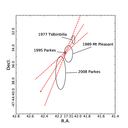
Figure 1: Published positions of B1727 obtained with various telescopes at different epochs as marked in the plot. Here and in other plots ellipse sizes correspond to the 1$\sigma$ coordinate uncertainties presented in Table 1 (39% 2D probability coverage). The Molonglo position (the first line in Table 1) has too large uncertainties and is not shown. The arrow and dashed lines show the p.m. vector and its uncertainties; the vector length shows the pulsar shift at a time base of 100 yr.

Table 2: Parameters of the two new glitches of B1727 found in this work

Epoch	$\Delta\nu_{\rm g}/\nu$	$\Delta\dot{\nu_{\rm g}}/\dot{\nu}$	$Q$	$\tau_{\rm d}$	Number	Data span
MJD, yr month	$10^{-9}$	$10^{-3}$		d	of ToAs	MJD
55735.18(14), 2011 Jun	53.6(1.2)	3.4(0.6)	0.125(0.014)	141(25)	37	55272–56214
56239.86(77), 2012 Nov	10.7(1.7)	1.7(1.9)	0.14(0.1)	70(96)	26	55897–56512

Note. —  $\nu=1/P$ is the pulse frequency, $\dot{\nu}$ is its first time derivative, $\Delta\nu_{\rm g}$ and $\Delta\dot{\nu_{\rm g}}$ are the changes of the frequency and its first derivative during the glitch, $\tau_{\rm d}$ is the exponential recovery time after the glitch, $Q$ is the ratio of the transient frequency increment to $\Delta\nu_{g}$ describing the fractional glitch recovery.

There exist five published positions of B1727 under the B1950 and/or J2000 coordinate systems measured with various telescopes at different epochs between 1972 and 2008 (Table 1).

As anticipated, the data show a noticeable positive increase in the R.A. and a negative trend in the decl. This is clearly seen in Figure 1, where the position from the first row of Table 1 for the epoch of 1972 is omitted because of large uncertainties. The linear fits to $\alpha$ (R.A.) and $\delta$ (decl.) coordinate changes over the epoch yield a formally significant “published-position” (PP) p.m.: $\mu_{\alpha}^{\rm PP}=63\pm 11$ mas yr^-1, $\mu_{\delta}^{\rm PP}=-83\pm 27$ mas yr^-1, and $\mu^{\rm PP}=104\pm 22$ mas yr^-1 with $\chi^{2}=1.6$ for 6 degrees of freedom (d.o.f.). The p.m. vector is shown by the arrow in Figure 1 with uncertainties (dashed lines). The backward extrapolation of the p.m. using the characteristic age of 80 kyr roughly points to the RCW 114 center. This p.m. results in the following transverse velocity of the pulsar $v_{\perp}=(1300\pm 200)\times D_{2.7}$ km s^-1, where $D_{2.7}$ is the distance in 2.7 kpc units. At the YMW16 DM distance of 5.5 kpc this is the record velocity, and the value is still quite large for the lower NE2001 DM distance of 2.7 kpc. To have a 2D speed in the typical for pulsars range 50$-$500 km s^-1 (e.g., Hobbs et al., 2005), B1727 should be substantially closer, namely at $\sim$0.5 kpc. This is consistent with the RCW 114 distance of $\lesssim 1.5$ kpc (Kim et al., 2010) thus favoring the association with the SNR.

This possibility, however, should be considered with a grain of salt as the differences in the reported coordinates can be just a result of unknown systematics between different telescopes$/$instruments. To confirm it, detailed analyses of homogeneous data sets are required.

The latter is possible as B1727 has been a permanent target of the Parkes 64 m telescope southern pulsar survey. Thanks to this, the timing analysis of the data obtained from 1990 to 2010 revealed four glitches in B1727 which occurred with intervals of about 2-5 yr (Yu et al., 2013, and references therein). Unfortunately, in addition to the frequent glitches, the pulsar shows a prominent timing noise hindering the p.m. measurement using a standard timing analysis. However, there are series of archival interferometric observations obtained in 2004–2005 and 2011 with the Australia Telescope Compact Array (ATCA) which can be used to verify the reliability of the timing p.m. derivations.

In the following sections we present the measurements of the p.m. of B1727 using the Bayesian method (Feroz et al., 2009; Lentati et al., 2014) on the available archival data collected with the Parkes telescope until 2014. We also use the ATCA archival data and our own observations obtained in 2016. Preliminary results of the analysis were briefly reported by Shternin et al. (2017). Here we also present two new pulsar glitches occurred between 2010 and 2014. The rest of the paper is organized as follows. The Parkes timing data and analysis are described in Section 3. In Section 4, we present the ATCA data and p.m. measurements. The p.m. results based on the published, timing, and interferometric data are concatenated in Section 5 and the association with RCW 114 is considered in Section 6. The results are discussed in Section 7 and summarized in Section 8.

3 Parkes timing data and analysis

The largest data set for the timing analysis of B1727 obtained with a single telescope is provided by the Parkes telescope archive. We selected the data obtained from 1993 February to 2014 March (MJD range 49043–56740). The detailed information on the observations and filterbank systems is given by Yu et al. (2013) who used the data obtained during the period between 1990 October and 2010 November (MJD range 48184–55507) partially overlapping with our adopted MJD range. We applied the PSRCHIVE tool (Hotan et al., 2004) to the archival data to obtain the pulse times of arrival (TOAs). As a result, 222 TOAs were obtained spanning 21 yr in total.

Table 3: Derived B1727 inter-glitch timing coordinates

Epoch	R.A., J2000	Decl., J2000	Interval range	Number
MJD, yr month			MJD	of TOAs
49203, 1993 Aug	17h31m42$.\!\!^{\rm s}$13(26)	$-$47∘44′37$.\!\!^{\prime\prime}$9(6.7)	49043.81$-$49363.21	20
50059, 1995 Dec	17h31m42$.\!\!^{\rm s}$09(2)	$-$47∘44′34$.\!\!^{\prime\prime}$55(52)	49415.05$-$50703.24	47
51590, 2000 Feb	17h31m42$.\!\!^{\rm s}$112(37)	$-$47∘44′36$.\!\!^{\prime\prime}$98(84)	50722.19$-$52458.51	33
53018, 2004 Jan	17h31m42$.\!\!^{\rm s}$169(21)	$-$47∘44′36$.\!\!^{\prime\prime}$78(49)	52484.38$-$53553.61	28
54659, 2008 Jul	17h31m42$.\!\!^{\rm s}$187(17)	$-$47∘44′37$.\!\!^{\prime\prime}$57(39)	53589.40$-$55730.53	63
55986, 2012 Feb	17h31m42$.\!\!^{\rm s}$225(92)	$-$47∘44′38$.\!\!^{\prime\prime}$0(1.8)	55759.45$-$56214.16	22
56497, 2013 Jul	17h31m42$.\!\!^{\rm s}$179(31)	$-$47∘44′38$.\!\!^{\prime\prime}$65(67)	56255.06$-$56740.76	18

Figure 2: Glitches in B1727. The pulse-frequency residuals $\Delta\nu$ (top), obtained by subtracting the (extrapolated) pulse frequency derived from the $\nu$ and $\dot{\nu}$ values of the first pre-glitch solution, and the variations of the pulse-frequency first time derivative $\dot{\nu}$ (bottom). The glitch epochs are indicated by vertical dashed lines. The last two glitches are found in this work, while the previous four are from Yu et al. (2013).

As the considered data span includes more recent observations than in Yu et al. (2013), we first searched for new glitches in B1727. To do that, we used the TEMPO2 timing package (Hobbs et al., 2006; Edwards et al., 2006) and followed the method described by Yu et al. (2013). As a result, we found two new glitches. Their parameters, shown in Table 2, are intermediate among those of the previous four glitches described by Yu et al. (2013). Variations of the pulse-frequency residuals $\Delta\nu$ and the pulse-frequency first time derivative $\dot{\nu}$ over the whole data span are presented in Figure 2 where the positions of all six glitches are marked by vertical lines.

With the glitch parameters in hands we turned to the inference of astrometric parameters. It is complicated by a strong timing noise of B1727. Several methods were developed to get rid of the timing noise. Recent approaches include a generalized least squares fitting developed by Coles et al. (2011) and the Bayesian approach realized in the TEMPONEST utility (Lentati et al., 2014). Li et al. (2016) recently showed that the two approaches give consistent results, especially for the p.m. measurements. Moreover, they argued that the novel timing analyzing techniques give results generally consistent with the interferometric measurements. In this work, we employ the TEMPONEST utility using two different approaches for the p.m. derivation to avoid possible bias.

In the first approach, we selected inter-glitch intervals to fit for the pulsar positions at the respective epochs. The resulting coordinates, epochs, interval ranges, and numbers of TOAs in the intervals are presented in Table 3. Two positions (MJD 50059 and MJD 54659) are for the same interglitch intervals as the already published positions (the last two rows in Table 1) and are compatible with them within the errors. Notice exclusively small errors for the MJD 50059 position published by Wang et al. (2000), which is presented in the 4-th row in Table 1 and shown in Figure 7 by the open diamond near the relative epoch of $-$3000. The authors applied a “polynomial whitening” method suggested by Kaspi et al. (1994). As has been discussed by Coles et al. (2011), in this approach the uncertainties, as a rule, are strongly underestimated. This is consistent with our findings for the same data (the second row in Table 3), where we get almost the same central value, but larger errorbars. At the same time, our uncertainties for the fifth interglitch interval are smaller than given in the last row in Table 1 because Yu et al. (2013) had less data for that interval than is available for us now.

Based on the positions in Table 3, we then derived the ‘inter-glitch’ (IG) p.m. using the linear fits as in Section 2. This resulted in $\mu_{\alpha}^{\rm IG}=67\pm 18$ mas yr^-1 and $\mu_{\delta}^{\rm IG}=-214\pm 40$ mas yr^-1 with $\chi^{2}=5.2$ for 10 d.o.f. The respective positions and the p.m. vector (thick arrow) are shown in Figure 3 where the p.m. uncertainties (thick dashed lines) are propagated from the average position at the mean epoch of June 2000. As seen, this result is in line with the “guess” provided by the published positions (cf. Figure 1), although the p.m. value $\mu^{\rm IG}=224\pm 38$ mas yr^-1 is about twice as large as compared with $\mu^{\rm PP}=104\pm 22$ mas yr^-1. The positional angle of the p.m.  vector defined from North to East is PA${}^{\mathrm{IG}}=161^{\circ}\pm 7^{\circ}$. It is slightly higher than the respective angle PA${}^{\mathrm{PP}}=141^{\circ}\pm 11^{\circ}$ derived from the published data.

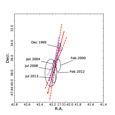
Figure 3: The same as in Figure 1 but for the Parkes timing positions of B1727 for six inter-glitch epochs listed in Table 3. The 1993 Aug position that has too large uncertainties is not shown. Thick and thin lines correspond to the p.m. measurements under the IG and GTS timing solutions, respectively, see text for details. The p.m. vector lengths for both solutions correspond here to the pulsar shift at a time base of 40 yr.

In the second approach we used the whole data span. The glitch parameters were, however, fixed in the TEMPONEST input as they have been derived at the initial analysis step. As a result, we obtained the “global timing-solution” (GTS) with the pulsar reference position R.A.=17^h31^m42$.\!\!^{\rm s}$14(1), decl.=$-$47^∘44^′36$.\!\!^{\prime\prime}$71(23) at a mid-span epoch of MJD 52892, and the p.m. $\mu_{\alpha}^{\rm GTS}=47\pm 14$ mas yr^-1, $\mu_{\delta}^{\rm GTS}=-133\pm 37$ mas yr^-1 at 68% confidence. The weighted post-fit rms residual was $\approx 202$ $\mu$s. Time variations of post-fit residuals shown in Figure 4 demonstrate the fit quality.

The GTS pulsar track is shown with the thin arrow in Figure 3 with uncertainties (thin dashed lines). For $\mu_{\alpha}$, both approaches provide compatible results within uncertainties. However, the p.m. in decl. direction is lower in the GTS solution than that in the IG solution at 90% confidence, resulting in somewhat lower overall $\mu$ value for the GTS solution. This demonstrates complications in accurate measurements of the astrometric parameters for noisy and glitching pulsars.

4 ATCA interferometric observations and data analysis

The first ATCA observations of B1727 were performed during a number of short sessions between 2004 December and 2005 March. We selected the data set obtained on 2005 March 26, with the $\approx$2h15m hour angle coverage. Although the coverage is short, this is the only session that allows for pulsar position measurements with a reasonable accuracy. The remaining shorter-coverage sets resulted in significantly larger position uncertainties and were found to be useless for our goals. The array was in the 6A configuration which contained baselines from 337 to 5939 m. The 128-MHz band was used with the central frequency of 1.384 GHz. In order to distinguish the pulsed emission from B1727 and background sources and boost signal to noise ratio for the pulsar data, the observations were performed exploiting the correlator pulsar binning capability.

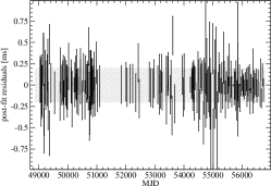
Figure 4: Timing post-fit residuals of the whole data span of B1727 after taking out the timing noise with the TEMPONEST. The hatched region represents the weighted post-fit rms residual of $\approx 0.2$ ms.

The next ATCA observations of the pulsar were obtained on 2011 November 19$-$20 as a part of The Compact Array Pulsar Emission Survey (CAPES). The observations were performed in the 16-cm band available with the Compact Array Broadband Backend (CABB) (Wilson et al., 2011) using the pulsar binning mode, with an hour angle coverage of about 11h. The band had a central frequency of 2.1 GHz and covered the spectral range of 1.1$-$3.1 GHz. The array configuration was 1.5D with baselines ranging from 107 to 4439 m.

In addition, we performed unscheduled observations of the pulsar on 2016 September 15 using Director’s time, that allowed for the $\approx$3h20m hour angle coverage. The data set was obtained with the same CABB frequency setup as in the 2011 observations, however the available array configuration H168 provided shorter baselines, from 61 to 4469 m, and no pulsar binning was possible.

Table 4: Interferometric coordinates of B1727 measured with the ATCA.

Date	R.A., J2000	Decl., J2000	$r1$	$r2$	PA	fpeak	$S/N$	$r1_{\mathrm{beam}}$	$r2_{\mathrm{beam}}$
			arcsec	arcsec	degrees	mJy		arcsec	arcsec
2005 Mar 26	17h31m42$.\!\!^{\rm s}$123(15)	$-$47∘44′36$.\!\!^{\prime\prime}$200(81)	0.167	0.021	$-$61.8	21.7(2)	118	32.7	4.1
2011 Nov 19$-$20	17h31m42$.\!\!^{\rm s}$212(5)	$-$47∘44′37$.\!\!^{\prime\prime}$022(67)	0.067	0.046	6.6	15.0(3)	45	5.0	3.5
2016 Sep 15	17h31m42$.\!\!^{\rm s}$263(9)	$-$47∘44′38$.\!\!^{\prime\prime}$276(160)	0.179	0.032	27.1	14.5(3)	43	13.1	2.3

Note. — $r1$, $r2$, and PA are the error ellipse radii and its position angle (North to East), respectively. $f_{\mathrm{peak}}$ is the pulsar peak value, $S/N$ is the pulsar signal to noise ratio, and $r1_{\mathrm{beam}}$ and $r2_{\mathrm{beam}}$ are the synthesized beam semi-axes. The beam PA is equal to the PA measured for the pulsar.

Three data sets described above were processed using the MIRIAD (Multichannel Image Reconstruction, Image Analysis and Display) package (Sault et al., 1995) following standard methods and the images were analyzed using Karma visualization tools (Gooch, 1996). The absolute flux density scale and bandpass calibration for all epochs were obtained from observations of PKS 1934$-$638, whereas the gain and phase instabilities were accounted using the 1657$-$56, 1714$-$397, and 1740$-$517 calibrators for the 2005, 2011, and 2016 data sets, which lie $\approx$ 9$.\!\!^{\circ}$75, 8$.\!\!^{\circ}$02, and 4$.\!\!^{\circ}$50 away from the target, respectively. In the case of the 2011 data, the primary calibration procedure revealed an unusual behavior of the YY polarization component that was visible across the bandwidth and affected all baselines. The cause of the problem remained unclear, but it could probably result from an unrecognized correlator issue. To avoid possible calibration problems, we thus used only the XX polarization for the analysis of this data set.

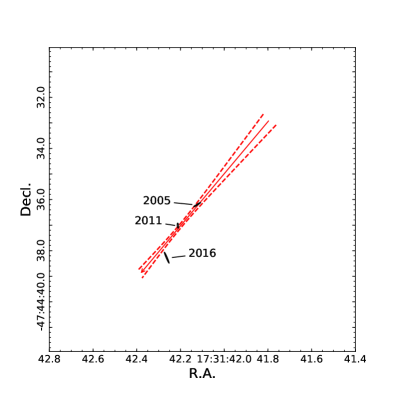
Figure 5: The ATCA interferometric positions of B1727 for the three epochs listed in Table 4. The p.m. track with uncertainties is shown for a 40 yr time base.

The data sets were imaged and deconvolved using standard routines. For the 2011 and 2016 data sets we used the MIRIAD mfclean deconvolution tool to account for spectral variations across the band. The variations were neglected in the 2005 data obtained in a much narrower bandwidth of 128 MHz and the MIRIAD clean tool was used. The pulsar positions were then measured on the respective full band on-pulse images of 2005 and 2011, and on the full band image of 2016 using the task imfit.

Table 5: The Cartesian components of the p.m. vector in R.A. ($\mu_{\alpha}$) and decl. ($\mu_{\delta}$) directions and the total p.m. value ($\mu$) and the position angle (PA). Different columns represent the p.m. results obtained by different methods.

Component	PP	IG	GTS	I	Irel	F	F1	Frel	F1rel
$\mu_{\alpha}$, mas yr-1	$63\pm 11$	$67\pm 18$	$47\pm 14$	$150\pm 10$	$81\pm 19$	$84\pm 4$	$87\pm 5$	$64\pm 7$	$66\pm 7$
$\mu_{\delta}$, mas yr-1	$-83\pm 27$	$-214\pm 40$	$-133\pm 37$	$-152\pm 8$	$-132\pm 23$	$-139\pm 7$	$-142\pm 7$	$-133\pm 14$	$-147\pm 14$
$\mu$, mas yr-1	$104\pm 22$	$224\pm 38$	$142\pm 34$	$213\pm 13$	$155\pm 29$	$162\pm 8$	$166\pm 9$	$148\pm 16$	$161\pm 17$
PA, deg	$141\pm 11$	$162\pm 6$	$159\pm 9$	$135\pm 4$	$148\pm 10$	$149\pm 2$	$148\pm 3$	$154\pm 5$	$156\pm 4$

Note. — Column names and methods: PP – using the published timing positions; IG – using the positions provided by the TEMPONEST timing solutions for the inter-glitch intervals; GTS – using the global timing solution provided by the TEMPONEST with the predefined glitch parameters; I – using the interferometry positions; I_rel – interferometry result in the ‘relative astrometry’ approach; F (F1) – final solution concatenating the PP, I, and GTS (IG) results. Notice, that the PP points used in concatenation do not include Parkes data already taken into account in GTS (IG) results to avoid double counting. Accordingly, F_rel (F1_rel) combines the PP, I_rel, and GTS (IG) results, see text for details. The errors correspond to the 68% confidence level.

The pulsar was firmly detected in all images with signal to noise ratios $S/N$ and peak fluxes $f_{\mathrm{peak}}$ given in Table 4. Notice the difference in $f_{\mathrm{peak}}$ for 1.384 GHz (2005 epoch) and 2.1 GHz (2011 and 2016 epochs) bands. The resulting pulsar coordinates with respective uncertainties are given in Table 4 and the position error ellipses are shown in Figure 5. According to the resulting positions, the pulsar demonstrates a significant regular shift between the 2005 and 2016 epochs which is compatible with shifts obtained from the timing measurements (cf. Figure 3). The resulted “interferometry” (I) p.m. values are $\mu_{\alpha}^{\rm I}=150\pm 10$ mas yr^-1, $\mu_{\delta}^{\rm I}=-152\pm 8$ mas yr^-1, and $\mu^{\rm I}=213\pm 13$ mas yr^-1. The $\delta$-component, which dominates the overall pulsar p.m., is consistent within uncertainties with the results of the timing analysis. In contrast, the $\alpha$-component is significantly larger than those found from the timing analysis, irrespective of which solution, IG or GTS, is adopted.

In Table 4 we quote purely statistical uncertainties which are roughly consistent with the expected ones calculated as a half of the synthesized beam size (given in the last columns in Table 4) divided by $S/N$. However, there can be systematic uncertainties exceeding the statistical ones. Partially, this can be guessed from Figure 5 where the position error ellipses seem not to follow the straight line and from a relatively large value of the $\chi^{2}=10$ for 2 d.o.f. for the proper motion fit. One source of the systematic errors is the absolute position uncertainties of the phase calibrators. Since three different calibrators were used, these errors are not canceled in the proper motion studies (as would have been if the same calibrator for all the epochs had been used). The calibrator position errors are negligible as compared to the pulsar position statistical errors in the 2005 data ($\approx$0.4 mas for 1657$-$56 ) and in the 2016 data ($\approx$8$\times$4 mas for 1740$-$517) while they appear to be noticeable for the 2011 data ($\approx$25$\times$52 mas for 1714$-$397). Adding the 1714$-$397 uncertainties in quadrature to the statistical ones leads only to a slight improvement of the fit ($\chi^{2}=8.7$), while the p.m. vector remains the same within the errors. Another source of systematic uncertainties can be related to the calibration and/or deconvolution algorithm errors. The most unreliable in this respect is the H168 array (2016 epoch) which has unbalanced baselines and is not well-suited for the astrometry tasks. The source of calibration errors can come from the antenna position uncertainties and incomplete compensation of the tropospheric/ionospheric propagation effects which are known to increase with the separation between the calibrator and the target (e.g., Chatterjee et al., 2004). These errors are difficult to estimate from the data as we have not found any cataloged radio source with precisely measured coordinates in the ATCA field of view.

However, these systematic errors can be estimated by comparing the positions of the uncatalogued sources between the epochs. By doing so we found considerable shifts between the positions of most of the point sources in the field. Therefore we followed the approach of Kirichenko et al. (2015) and performed the relative astrometry of the ATCA images using as the reference the positions of eight point sources around the pulsar firmly detected in all the images. The details of the procedure are given in Appendix A. In short, we allowed for shifts and rotations between the images as well as for an overall scaling. The astrometric solution revealed $\approx 0\hbox{$.\!\!^{\prime\prime}$}6$ shift in R.A. between the 2005 and 2011 images and $\approx 0\hbox{$.\!\!^{\prime\prime}$}6$ shift in decl. between the 2011 and 2016 images. Moreover, the successful solution was obtained only when the 2011 image was scaled by a factor of $\approx 0.998$. The most likely cause of the latter factor is related to the additional frequency averaging performed by CABB in the pulsar binning mode. After applying this transformation, the positions of the reference sources agreed well between the epochs (see Appendix A). In this way we lose the information on the absolute positions of the pulsar (and the reference sources) but can estimate its proper motion. As a result, we found $\mu_{\alpha}^{\mathrm{I}_{\mathrm{rel}}}=81\pm 19$ mas yr^-1 and $\mu_{\delta}^{\mathrm{I}_{\mathrm{rel}}}=-132\pm 23$ mas yr^-1. While the decl. component is consistent within errors with the estimate based on the absolute (more precisely, relative to the calibrators) interferometric positions, the R.A. component decreased significantly. Notably, this ‘relative astrometry’ p.m. estimate is consistent within 1-2$\sigma$ with the various timing-based estimates discussed above.

5 Concatenation of the published, timing, and interferometric p.m. results

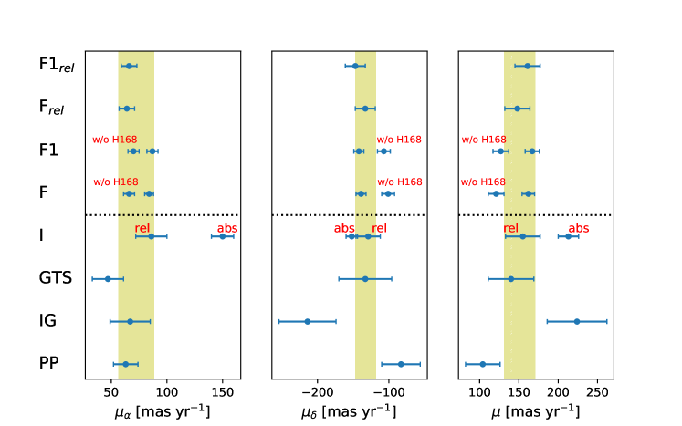
Figure 6: Summary of the proper motion measurements using various methods described in the paper. Dotted line separates the independent measurements (below) and the results from different approaches to their combination (above). Vertical strips show our final conservative p.m. estimate, see text for details.

In Table 5 and Figure 6, we collect all p.m. measurements based on the published positions (Section 2), the Parkes timing positions (Section 3), and the ATCA interferometry positions (Section 4). Despite differences in some of the p.m. components, all approaches result in substantial proper motion roughly in the same direction. To get the most robust pulsar astrometry it is useful to consider all the data together.

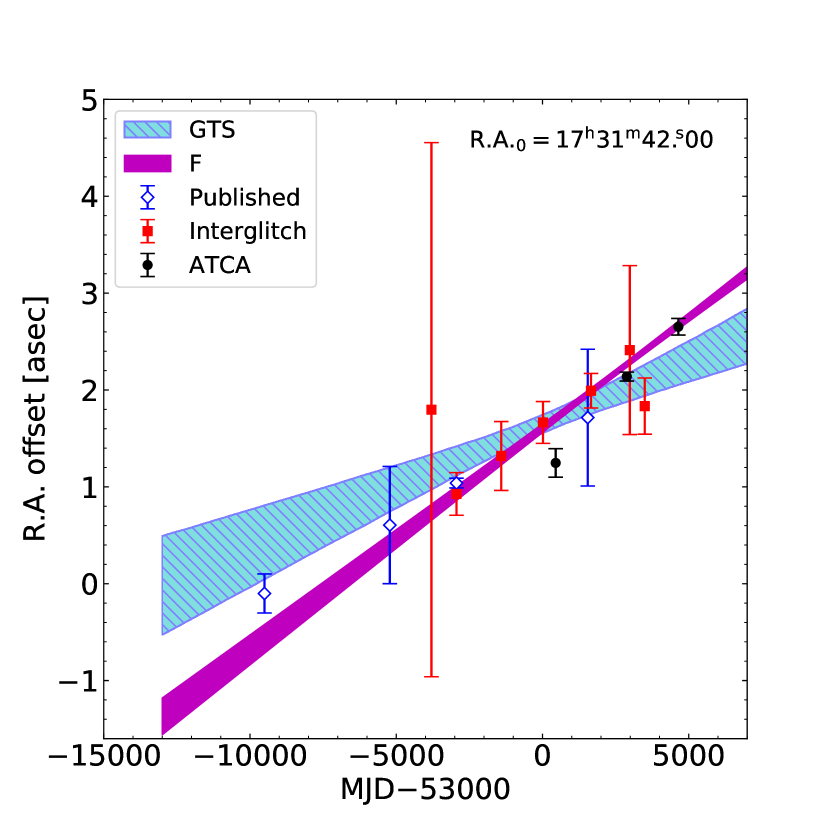
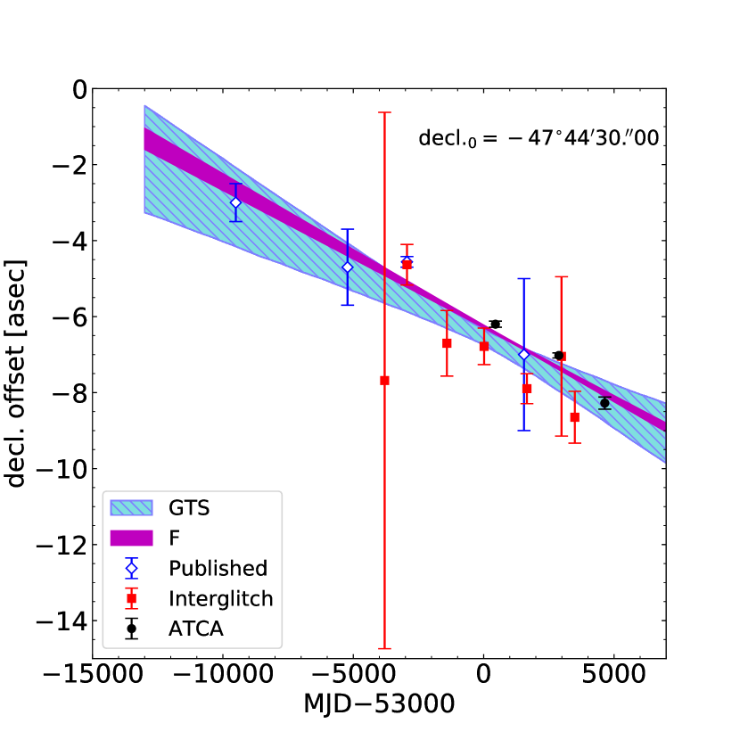
Figure 7: B1727 R.A. (left) and decl. (right) variation with the epoch based on the published (open diamonds), and our timing inter-glitch (filled squares) and ATCA interferometric (filled circles) positions measured at different epochs. The coordinates are presented in offsets relative to a reference point with RA₀ and decl.₀ shown in the plots. The epoch axis is referenced to MJD 53000. Hatched and filled strips show 68% credible regions for the pulsar p.m. track based on our global timing solution and on our combined solution F, respectively.

In Figure 7, we plot the published pulsar coordinates (Table 1), inter-glitch coordinates (Table 3), and interferometry coordinates (Table 4) by the open diamonds, squares, and circles, respectively. The earliest position, corresponding to the first row in Table 1, has too large uncertainties and is not shown. The position epochs are referenced to the MJD 53000, and the coordinates are shown in relative offsets from an auxiliary reference point with R.A.₀ and decl.₀ as indicated in the plots. Hatched strip in Figure 7 shows the 68% credible region for the pulsar track based on our global timing solution obtained with TEMPONEST in Section 3. As seen, all data points, including the published and interferometric ones, are consistent with each other for the same epochs and with the GTS region at $1-2\sigma$ level.

However, there is a clear tension between the interferometric p.m. in the R.A. direction as measured relative to the calibrators, $\mu_{\alpha}^{\mathrm{I}}$, and other measurements, which is best seen in Figure 6. In this Figure, the p.m. components based on the ‘absolute’ ineterferometric positions are marked by ‘abs’. Indeed, fitting the linear pulsar track using the interferometric positions, the timing inter-glitch positions, and the two published positions before MJD 49043 (excluding again the Molonglo point) together, we obtain the “F1” solution presented in Table 5 and Figure 6. However, since the interferometric fit is not good, the “F1” fit is not good either, with $\chi^{2}=76$ for 20 d.o.f. Taking out the H168 position (epoch 2016) we obtain a much better fit with $\chi^{2}=28$ for 18 d.o.f. ($p$-value of 6.2%). In this case, which is marked with ‘w/o H168’ labels in Figure 6 and not shown in Table 5 for brevity, $\mu_{\alpha}=70\pm 5$ mas yr^-1 and $\mu_{\delta}=-107\pm 9$ mas yr^-1.

It is not possible to combine our favored GTS timing solution with other positions in the similar fashion, since the former results from the Bayesian analysis of the whole TOAs dataset based on the Markov Chain Monte Carlo simulations which return the sample from the posterior distributions of the pulsar position at the reference epoch and the proper motion parameters. These posteriors need to be updated with the information on the interferometric and published positions. To do this, we approximated the joined posterior distributions of the four astrometric parameters marginalized over other model parameters with the multivariate normal distribution which works well for our TEMPONEST result. This approximated posterior was then used in combination with likelihoods for other positions assuming the pulsar linear motion to obtain the updated inference on the parameters. This resulted in the ‘F’ proper motion solution also shown in Table 5 and Figure 6. It gives $\mu_{\alpha}^{\mathrm{F}}=84\pm 4$ mas yr^-1 and $\mu_{\delta}^{\mathrm{F}}=-139\pm 7$ mas yr^-1, consistent with the ‘F1’ solution based on the inter-glitch timing positions. Although it is not straightforward to extract the goodness-of-fit for this solution, we expect that the situation is similar to the ‘F1’ case, i.e. the tension between the I positions and the GTS solution results in a bad combined fit. This is illustrated with the filled strip in Figure 7 which shows the pulsar track under the ‘F’ solution and its 68% uncertainty range. Its R.A. part (left panel) deviates either from the GTC and the interferometric position. Performing the same fit without H168 position gives $\mu_{\alpha}=66\pm 5$ mas yr^-1 and $\mu_{\delta}=-142\pm 7$ as marked with ‘w/o H168’ in the ‘F’ row in Figure 6. This is consistent with the respective ‘F1 w/o H168’ solution.

The interferometric results I_rel based on the direct registration of the images for three ATCA epochs can be considered as more robust and less affected by the systematic calibration errors than the ‘I’ results. Since the information about the absolute position is lost during the registration procedure, it is impossible to combine the results of timing and interferometric analysis based on the pulsar positions as above. Instead, we combined the timing solution, IG or GTS, with the two published positions and then took the weighted means of the resulting p.m. component values with the respective I_rel components. In this way we get the final ‘F_rel’ and ‘F1_rel’ solutions in Table 5 and Figure 6, based on the GTS or IG timing results, respectively. These two results are consistent with each other and with timing and I_rel values. Based on the discussion in Sections 3–4, we suggest the F_rel as the most reliable proper motion solution, that accounts in the best way for the timing noise in the Parkes data and the systematics in the ATCA data.

To be more conservative, however, we will further consider the extended region which contains both the F and the F_rel solutions as our final p.m. estimate as indicated with the filled vertical strips in Figure 6. This range is also in agreement with the results obtained by exclusion of the H168 data point and with the results obtained by doubling the ATCA position errors (not shown for brevity). Therefore, our conservative estimate is $\mu_{\alpha}=73\pm 15$ mas yr^-1 and $\mu_{\delta}=-132\pm 14$ mas yr^-1 resulting in the total p.m. $\mu=151\pm 19$ mas yr^-1 in the direction specified by the position angle $\mathrm{PA}=151^{\circ}\pm 8^{\circ}$. This yields the pulsar transverse velocity $v_{\perp}=(1930\pm 240)\times D_{2.7}$ km s^-1.

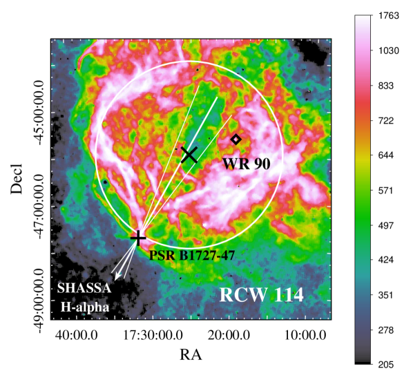
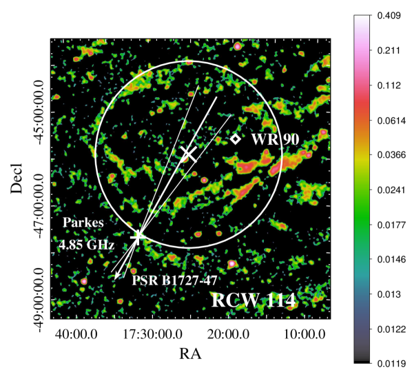
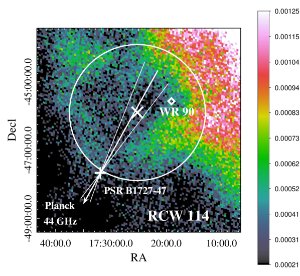
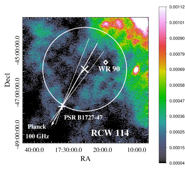
Figure 8: RCW 114 SNR images obtained in the H$\alpha$ emission line (The Southern H$\alpha$ Sky Survey Atlas (SHASSA); Gaustad et al., 2001), at 4.85 GHz (The Parkes-MIT-NRAO Southern Sky Survey; Condon et al., 1993), and 44 and 100 GHz (Planck Release 1 results) as notified in the frames. Colours show the intensity in photons cm^-2 s^-1 sr^-1, in Jy beam^-1, and in antenna temperatures (K), for the H$\alpha$, 4.85 GHz, and Planck images, respectively. In each frame, the circle of a 2^∘ radius roughly outlines the presumed outer shell of the SNR as seen in H$\alpha$; the X-point is the circle center. The diamond marks the position of the WR 90 star projected on the remnant. The B1727 position is shown by the cross. Its p.m. track is presented by the arrow, which is extended backwards by the characteristic age (80 kyr); thin lines show 1$\sigma$ uncertainties of the track.

6 Association with RCW 114

In the top left panel of Figure 8, we show the H$\alpha$ image of the extended RCW 114 nebula whose shell structure is thought to represent an evolved SNR (see discussion in Section 7.1 below). Three other panels of Figure 8 show radio images of RCW 114 at 4.85 GHz (top right panel), 44 GHz (bottom left panel), and 100 GHz (bottom right panel). In H$\alpha$, the shell-like structure of the nebulae with a radius of $\approx$ 2^∘ is clearly seen. In addition, three almost parallel ridges cross over the south-west SNR quadrant. Faint radio filaments spatially correlated with the bright H$\alpha$ shell and the ridge features can be resolved in the 4.85 GHz radio map. Although they are only barely resolved at lower frequencies (Duncan et al., 1997), the overall shell-like structure of RCW 114 is visible at higher frequencies until 100 GHz in the Planck telescope data (bottom panels in Figure 8).

B1727 position coincides with the south-east shell of this remnant, as shown by the plus sign in Figure 8. To check for the possible association between the pulsar and the SNR, we performed a backward extension of the B1727 p.m. track, using the final p.m. vector measured in Section 5 and the pulsar characteristic age of 80 kyr. We checked that the pulsar track distortion due to the Galactic gravitational potential is negligible at such a short time scale. This extension is shown by the arrow in Figure 8, while thin lines bracket the 68% extrapolation uncertainty propagated from the measured p.m. uncertainty. The pulsar track passes remarkably close to the putative RCW 114 shell center marked with the ‘x’-point in Figure 8 and shows that B1727 was at least born at a position within the remnant. Moreover, if the pulsar was born at the remnant center, its age should be about 50 kyr, which is a reasonable value provided that pulsar characteristic ages usually differ from their true ages, when the latter are known (Thorsett et al., 2003; Popov & Turolla, 2012). Difference between the inferred kinematic age and the pulsar characteristic age allows to constrain its initial period. We save this discussion to Section 7.3.

Thus we can conclude that the p.m. measurements of B1727 strongly support the genuine association between the PSR and the SNR. In this case the most plausible age of the PSR+SNR system is about 50 kyr.

7 Discussion

7.1 Nature of the RCW 114 nebula

For a long time the SNR nature of RCW 114 was not obvious. Historically, one of the counterarguments was the absence of the radio and soft X-ray emission typical for SNRs (Bedford et al., 1984). However, Parkes and Planck data shown in Figure 8 reveal faint radio emission spatially correlated with the nebula optical features. In X-rays, RCW 114 has not yet been detected. Nevertheless, in the far-ultraviolet, the emission in the C iv line spatially correlated with the H$\alpha$ features was found (Kim et al., 2010). This situation is possible in evolved SNRs where the excited matter has already cooled down enough to be undetectable in X-rays while it can still be visible in the ultraviolet (Shelton, 1999). Moreover, spectroscopic studies of the optical filaments in RCW 114 (Walker & Zealey, 2001) revealed high S ii/H$\alpha$ line ratios, which are consistent with those produced by a supernova shock in interstellar matter (ISM; Fesen et al., 1985).

According to the alternative interpretation (e.g, Cappa de Nicolau et al., 1988; Welsh et al., 2003), RCW 114 could be an asymmetric bubble blown in ISM with a density gradient by the wind from a Wolf-Rayet star HD 156385, also known as WR 90. In Figure 8, the WR 90 location is marked by the diamond. However, analyzing H i 21 cm maps that had better resolution than those used in the older studies, Kim et al. (2010) found two H i voids in the direction of RCW 114. The prominent H i void already found by Cappa de Nicolau et al. (1988) has a systemic velocity of $\approx-4$ km s^-1, whereas the velocity of a smaller circular-shaped void around WR 90 is $\approx-13$ km s^-1. The latter structure of about 50^′  in diameter is apparently visible in the H$\alpha$ and Planck images in Figure 8 as well. The prominent void can be identified with RCW 114, while the smaller void corresponds to the WR 90 wind-blown bubble. The difference in velocities suggests that RCW 114 is unrelated to WR 90 and, in addition, is closer to us (Kim et al., 2010).

Combining all the facts, we can confidently consider RCW 114 as an evolved SNR. Clearly, the presence of the neutron star, B1721, kicked roughly from the RCW 114 center, also favors the SNR interpretation.

It is possible to get an estimate on the distance to the RCW 114 analyzing the spectral properties of the stars projected on the remnant. This was done by Welsh et al. (2003) who observed the interstellar Na i D1 & D2 Fraunhofer absorption lines in spectra of seven field stars located within the distance range of 0.2–1.5 kpc. We updated their analysis using recent Gaia parallax-based distance measurements for these stars (Bailer-Jones et al., 2018). In Figure 9 we show the D1 & D2 equivalent widths vs. stars’ distances based on the figure 3 in Welsh et al. (2003). The prominent equivalent width excess at $D\gtrsim 1.1$ kpc is much better localized as compared to the initial version by Welsh et al. (2003). Four nearby stars with $D\lesssim 0.5$ kpc, including HD 157698 with a distance of $0.43^{+0.020}_{-0.018}$ kpc, show a single component absorption profile indicating that they are foreground objects for RCW 114. The next by the distance star, HD 157832 ($D=1.078^{+0.092}_{-0.079}$ kpc), shows a broader double component profile demonstrating that it is already behind (or within) the SNR. The WR 90 distance derived from recent Gaia parallax measurements is $1.154^{+0.082}_{-0.072}$ kpc (Bailer-Jones et al., 2018). This star, and HD 156575 ($D=1.268^{+0.084}_{-0.074}$ kpc), show even more complex multi-component structures of line profiles, with larger equivalent widths. A similar pattern was found in the IUE spectra of the interstellar Si ii $\lambda 1304$ absorption line profiles (Welsh et al., 2003). This can be interpreted as a result of the contribution from both the RCW 114 filaments and the expanding WR 90 wind bubble (Kim et al., 2010). Notice that both WR 90 and HD 156575 project on the smaller H i void (Kim et al., 2010), while HD 157832 does not. The complexity of the profiles is thus consistent with the H i data also suggesting that WR 90 wind bubble is further than RCW 114 (Kim et al., 2010). The spectroscopic analysis results in the 0.4–1.1 kpc distance range for the RCW 114 which is shown in Figure 9 by the double-ended arrow. This distance range is in accord with the limit of $\lesssim 1.5$ kpc based on the assumption that the C iv luminosity can hardly exceed the luminosity of Cygnus Loop (Kim et al., 2010). Observations of interstellar absorption features in spectra of field stars with the distances within the range of 0.5–1 kpc, filling the distance gap in Figure 9 between HD 157698 and HD 157832, can help to better constrain the distance to the SNR.

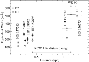
Figure 9: Interstellar Na i D1 & D2 absorption line equivalent widths vs parallax-based distances for seven stars projected on RCW 114. The star names are shown near their data-points, the line widths are taken from Welsh et al. (2003), and the parallaxes are measured with Gaia. The width excesses for WR 90 and HD 156575 are caused by the interstellar absorption associated with RCW 114 and the WR 90 H i bubble. A plausible distance range for RCW 114 is shown by the double-ended arrow.

7.2 RCW 114 vs SNR models, its ambient ISM density and evolution phase

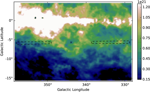
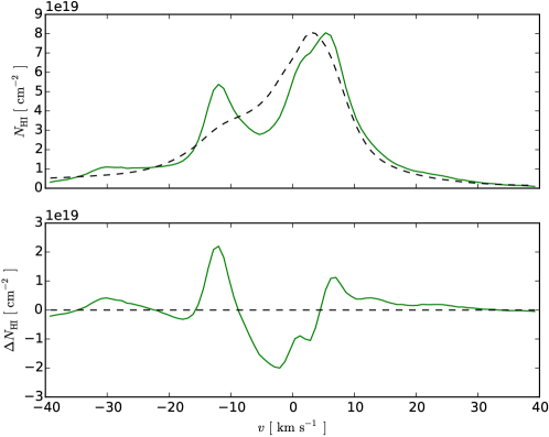
Figure 10: Top: GASS map of the H i emission towards the RCW 114 SNR in units of $N_{\textrm{H}\,\textsc{i}}$ marginalized over the LSR velocities $-8\,{\rm km\,s^{-1}}<v<+1\,{\rm km\,s^{-1}}$. RCW 114 is associated with the void whose approximate center is marked by the cross. Dashed polygons show regions selected for the background extraction. Middle: The solid and dashed lines show the column density velocity profiles extracted along the direction marked by the cross and the background regions in the top panel, respectively. Bottom: The difference of the two curves in the middle panel which reveals two ISM peaks and a void between them produced by the SNR shock.

It is important to check if the pulsar-SNR association is consistent with the observed RCW 114 properties. The distance range of $0.4-1.1$ kpc and the angular diameter of 4^∘ imply the remnant radius in the range of $16-35$ pc. Proper motion arguments suggest that the age of the system is about $50$ kyr (Section 5). Both values are above the upper limits of $\approx$14 pc and $\approx$13 kyr constraining the Sedov-Taylor SNR expansion phase (e.g., Cioffi et al., 1988). Therefore the remnant has likely entered the next pressure-driven snowplough (PDS) phase.

The analytical expressions for the PDS expansion phase in a uniform ambient ISM with Solar abundances from Cioffi et al. (1988) result in the following approximate estimates for the SNR blast-wave shock velocity $V_{\rm s}$ and radius $R_{\rm s}$

$$V_{\rm s} \approx 134~{}{\rm km}~{}{\rm s}^{-1}\times E_{51}^{0.22}n_{0}^{-0.26}\left(\frac{t}{50~{}{\rm kyr}}\right)^{-0.7},$$

$$R_{s} \approx 22~{}{\rm pc}\times E_{51}^{0.22}n_{0}^{-0.26}\left(\frac{t}{50~{}{\rm kyr}}\right)^{0.3},$$ (2)

where $E_{51}$ is the supernova explosion energy in $10^{51}$ erg units, $n_{0}$ is the pre-supernova particle number density of the ambient ISM in cm^-3, and $t$ is the SNR age. At $t\gtrsim 20$ kyr, Equations (LABEL:eq:vpds)–(2) are consistent with more complex expressions by Cioffi et al. (1988) within a few per cent accuracy. For the the remnant angular radius of about 2^∘, Equation (2) implies the distance

$$D \approx 647~{}{\rm pc}\times E_{51}^{0.22}n_{0}^{-0.26}\left(\frac{t}{50~{}{\rm kyr}}\right)^{0.3}.$$ (3)

For reasonable values of $E_{51}$, $n_{0}$, and $t$, it is in accord with the 0.4–1.1 kpc range obtained in Section 7.1.

In order to further analyze Equations (LABEL:eq:vpds)–(3), we tried to independently estimate $n_{0}$ using the third data release of the Parkes Galactic All Sky Survey (GASS) of the Milky Way H i emission (Kalberla & Haud, 2015). The top panel in Figure 10 shows the H i map of the RCW 114 region summed up over the the local standard of rest (LSR) velocity range $-8$ km s^-1 $<v<$ $+1$ km s^-1. The map is converted to the column density $N_{\textrm{H}\,\textsc{i}}$ using the expression $N_{\textrm{H}\,\textsc{i}}=1.822\times 10^{18}\Delta vT(v)$ cm^-2, where $T(v)$ is the brightness temperature in Kelvins and $\Delta v$ is the velocity channel width in km s^-1 (see, e.g., Matthews et al., 1998). An extended H i void is seen in the map which coincides by its position and morphology with RCW 114 (cf. Figure 8), as discussed in Section 7.1. It presumably corresponds to a cavity in the ISM swept up by the passage of the SNR shock. An approximate void center is marked by the cross.

The $N_{\textrm{H}\,\textsc{i}}$ velocity profile extracted from the data using the direction towards the center is shown in the middle panel of Figure 10 by the solid line. There is a dip in the profile between $-$10 km s^-1 and 5 km s^-1 excavated by the shock. The corresponding deficit of $N_{\textrm{H}\,\textsc{i}}$ divided by the SNR extent along the direction would give us an estimate of the initial density of the ISM where the supernova exploded in. However, to estimate the deficit correctly, the background gas has to be taken into account. To estimate the background, we take an average of $N_{\textrm{H}\,\textsc{i}}$ from two dashed polygons located outside the SNR and stretched along the Galactic longitude (see the top panel of Figure 10). The background velocity profile is shown by the dashed line in the middle panel of Figure 10, while the background-subtracted profile towards the SNR center is presented in the bottom panel of Figure 10. Two peaks or walls which are presumably formed by the material swept up by the SNR shock and a void between them are seen in the subtracted profile. The total $N_{\textrm{H}\,\textsc{i}}$ deficit between the two walls is $\approx 1.9\times 10^{20}\,\rm cm^{-2}$. The ambient matter density can be now estimated as $n_{0}=N_{\textrm{H}\,\textsc{i}}/(2R_{s})$. Notice that $R_{s}$ in Equation (2) itself depends on $n_{0}$.

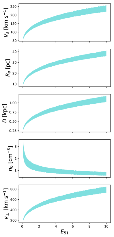
Figure 11: Dependencies of the RCW 114 SNR parameters on the supernova explosion energy $E_{51}$. Panels show (from top to bottom) the expansion velocity $V_{s}$, the remnant radius $R_{s}$, the distance to the system $D$, the ambient matter density $n_{0}$, and the pulsar transverse velocity $v_{\perp}$ at the remnant distance. See text for details.

This estimate allows us to exclude $n_{0}$ from Eqs. (LABEL:eq:vpds)–(3), and the remnant properties are then parameterized only by the explosion energy $E_{51}$. In Figure 11 we show the dependencies of the parameters $V_{s}$, $R_{s}$, $D$, and $n_{0}$ on $E_{51}$ taking into account uncertainties in various constraints on parameters employed. The bottom panel in Figure 11 additionally shows the pulsar transverse velocity $v_{\perp}$ at the RCW 114 distance. Specifically, to obtain the uncertainty strips plotted in Figure 11, we included $0\hbox{$.\!\!^{\circ}$}1$ uncertainty on the remnant angular radius, $0\hbox{$.\!\!^{\circ}$}3$ uncertainty on the pulsar shift during lifetime (this, combined with the B1727 p.m., gives the system age, cf. Section 6), and 20% accuracy of our $N_{\textrm{H}\,\textsc{i}}$ deficit estimate. As can be seen from Figure 11, our adopted distance range of $0.4-1.1$ kpc corresponds to a broad explosion energy range of $(0.3-10)\times 10^{51}$ erg.

Typical explosion energies obtained in simulations of neutrino-driven core-collapse supernovae are about $(0.5-1.5)\times 10^{51}$ erg (Sukhbold et al., 2016; Müller et al., 2016). This puts RCW 114 at the lower edge of the adopted distance range. For instance, for $E_{51}=1$ the dependencies shown in Figure 11 result in $V_{s}=120\pm 10$ km s^-1, $R_{s}=19\pm 1$ pc, $D=550\pm 40$ pc, $n_{0}=1.4\pm 0.3$ cm^-3, and $v_{\perp}=397\pm 30$ km s^-1. Most of the simulations suggest an explosion energy upper limit of about $2\times 10^{51}$ erg for of the core-collapse neutrino-driven supernovae (Janka, 2012; Müller, 2017, and references therein) (see, however, Pejcha & Thompson, 2015). As follows from Figure 11, at $D\gtrsim 750$ pc the RCW 114 explosion energy should be higher than this limit, which in turn means that a non-standard explosion mechanism, e.g., a magneto-rotational supernova, needs to be invoked in this case. This suggests that the lower half of the adopted distance range, i.e., 400–750 pc, is somewhat more probable.

At the same time, the estimated shock speeds are $V_{\rm s}>95$ km s^-1 (top panel in Figure 11) which is hard to reconcile with the expansion velocities of 25–35 km s^-1 obtained in the analysis of the radial velocities measured in the optical for a few RCW 114 filaments (Meaburn et al., 1991). This is not unusual that the radial speeds measured in the remnant filaments are smaller than the real expansion speed. In this case, the lower-speed motion of the filaments may be driven by a secondary remnant shock. A similar situation is observed, e.g., for another evolved SNR S147 associated with PSR J0538$+$2817. In this case, the maximal measured velocity is about 100 km s^-1 while most filaments show significantly smaller velocities, with a mean value of 10 km s^-1 (e.g., Ren et al., 2018, and references therein). Moreover, for one faint filament located at the south-east edge of the RCW 114 remnant, Meaburn et al. (1991) found a high velocity H$\alpha$ component centered at 80 km s^-1 with the line width of about 30 km s^-1. If it is associated with the remnant expansion, the real expansion speed should be higher due to the projection arguments. This is in agreement with the calculated $V_{\rm s}$ range.

7.3 Pulsar birth period

The independent estimation of the pulsar age based on the derived p.m. and the PSR-SNR association allows one to probe its initial period. For the power-law spin-down evolution with a braking index $n$, the pulsar initial period can be found from the true age $\tau$ and the current period $P$ as (e.g., Lorimer & Kramer, 2012)

$$P_{0}=P\left[1-\frac{n-1}{2}\frac{\tau}{\tau_{c}}\right]^{1/(n-1)}.$$ (4)

The purely magnetic dipole braking mechanism corresponds to $n=3$. Then, assuming $\tau=50\pm 10$ kyr, we get $P_{0,3}=0.5\pm 0.1$ s (here we follow the notation of Noutsos et al. (2013) where the second number in the initial period superscript, if present, corresponds to the adopted value of $n$). Braking indices are rarely known well. In cases when the braking indices are reliably measured, they are less than 3, making the simple dipole spin-down model inadequate. Since B1727$-$47 has a lot of glitches and timing noise, it is hardly possible to firmly estimate $n$ ($\ddot{\nu}$) from timing solution. Allowing $n$ to vary in the range of $1.4-3$ we get $P_{0}=0.56\pm 0.07$ s, where the error is dominated by the age uncertainty and not by the adopted index range. Therefore, if the supernova explosion was highly asymmetric with the pulsar birth site significantly shifted from the SNR geometric center, B1727$-$47 could be older and thus faster rotating at birth.

The inferred initial period of B1727$-$47  is quite large as compared to the $P_{0}$ values of 30 young pulsars whose real ages were more or less reliably estimated via their associations with SNRs (Popov & Turolla, 2012). With a few exceptions, their initial periods cluster at $P_{0,3}\lesssim 0.1$ s. Noutsos et al. (2013) analyzed kinematic ages of 27 pulsars and found a bimodal distribution of pulsars over $P_{0,3}$. The long-period component formed by a half-dozen of pulsars is located at $P_{0,3}>0.6$ s. B1727$-$47 could belong to this population. However, its members are significantly older, $>10^{5}$ yr, than B1727$-$47 as well as the sample presented by Popov & Turolla (2012). It is not impossible that the appearance of this population in the analysis by Noutsos et al. (2013) is related to the pulsar magnetic field evolution and does not resemble the actual initial period distribution (Igoshev & Popov, 2013). B1727$-$47 is young and as such, the longer term evolution of the magnetic field can hardly affect its initial period estimate.

There are only two objects in the Popov & Turolla (2012) sample that have $P_{0,3}>0.4$ s. One of them, PSR J1210$-$5225 associated with the SNR G296.5$+$10, is a weakly-magnetized, $B\sim 10^{11}$, slowly rotating pulsar dubbed “anti-magnetar” (e.g., Gotthelf et al., 2013; Halpern & Gotthelf, 2015, and references therein). It is also known as CCO 1E1207+5209 and is a peculiar object in comparison to a bulk of NS populations (see, e.g., De Luca, 2017, for review). In contrast, the second source, PSR B2334$+$61 associated with the SNR G114.3$+$0.3, is quite similar to B1727$-$47. It has $B\approx 10^{13}$ G, the period $P=0.49$ s, and a characteristic age of $40$ kyr. Similarly to B1727$-$47, its association with the SNR suggests a lower distance than inferred from the electron density maps and a smaller true age $\tau\sim 10$ kyr (Yar-Uyaniker et al., 2004). The latter translates to $P_{0,3}\approx 0.9P=0.45$ s, which is remarkably close to our estimate for B1727$-$47. On the other hand, only a marginal p.m. of $\mu_{\alpha}=-1\pm 18$ mas yr^-1 and $\mu_{\delta}=-15\pm 16$ mas yr^-1 is reported for PSR B2334+61 (Hobbs et al., 2005) resulting in a 3$\sigma$ upper limit of the transverse velocity $v_{\perp}<230D_{0.7~{}\mathrm{kpc}}$ km s^-1, where $D_{0.7~{}\mathrm{kpc}}$ is the distance to PSR B2334$+$61 scaled by the favored distance of 0.7 kpc (Yar-Uyaniker et al., 2004). Although somewhat smaller, this value is nethertheless comparable to the transverse velocity inferred for B1727$-$47.

Recent simulations of the core-collapse supernovae by Müller et al. (2019) revealed a significant anti-correlation between NS $P_{0}$ and $v_{\perp}$. On the other hand, parametric simulations by Wongwathanarat et al. (2013) resulted in the initial periods in the range of $0.1-8$ s and the birth kick velocities up to more than $700$ km s^-1 (due to a so-called “tug-boat” mechanism) without any apparent correlation between the two parameters. The relatively large initial periods accompanied by the large kick velocities inferred for B1727$-$47, and partially for PSR B2334$+$61, appear to be challenging for both simulations, which make these two pulsars important tests for the core-collapse supernova models.

7.4 Pulsar distance and the Galactic electron density distribution

Current models of the electron density distribution in the Galaxy place B1727 either at the DM distance of 2.7 kpc (NE2001 model; Cordes & Lazio, 2002) or even at 5.5 kpc (more recent model by Yao et al., 2017). According to our p.m. measurements (Section 5), both models result in an unrealistically high transverse velocity $v_{\perp}$ of about 2000 or 4000 km s^-1, respectively. Typical pulsar transverse velocities are in the range of $50-700$ km s^-1 (Brisken et al., 2003; Hobbs et al., 2005; Faucher-Giguère & Kaspi, 2006; Verbunt et al., 2017; Jankowski et al., 2019) suggesting that B1727 is much closer than the electron density models predict. This is again in line with the picture of the association of B1727 with RCW 114, see the bottom panel in Figure 11. The adopted RCW 114 distance range of 0.4–1.1 kpc results in the pulsar $v_{\perp}$ in the range of 300–800 km s^-1, with the higher plausibility being granted to its lower end. This makes the pulsar velocity a typical one, supporting further the PSR-SNR association. As stated above, such a value of the pulsar velocity can be explained by the standard pulsar kick mechanisms (e.g., Janka, 2017, and references therein). In this case, however, the existing models of the Galactic electron density distribution require serious corrections in the direction to the pulsar.

An independent support for the smaller distance comes from the recent $\gamma$-ray detection of B1727$-$47 (Smith et al., 2019). The $\gamma$-ray efficiency $\eta=L_{\gamma}/\dot{E}$, i.e. the ratio of the $\gamma$-ray luminosity to the spin-down energy, is found to be 80% for the distance of 2.7 kpc and more than the limiting 100% for the 5.5 kpc (assuming the $\gamma$-ray beaming factor $f_{\Omega}=1$). In contrast, at the distances less than $1$ kpc, one obtains $\eta\lesssim 11\%$, the value typical for the $\gamma$-ray pulsars. Therefore, the $\gamma$-ray observations also point out to the overestimation of the B1727$-$47 distance by the current electron density models, although the possibility of a strong beaming ($f_{\Omega}\ll 1$) or an unknown contamination of the observed $\gamma$-ray flux by RCW 114 can somewhat lighten these arguments (Smith et al., 2019).

The discussion above implies that the fractional uncertainty of the models of the Galactic electron density distribution along the pulsar line of sight is 60–80%. Such a situation is not unusual (Yao et al., 2017). For instance, the very long baseline interferometry (VLBI) parallax measurements for two pulsars revealed 65% lower distances than followed from the NE2001 model (Kirsten et al., 2015). Subsequent extensive VLBI parallax analysis of 57 pulsar under the PSR$\pi$ project also suggests that the accuracy of the DM-based distance predictions is significantly overestimated (Deller et al., 2018). Using precise timing observations of 42 millisecond pulsars, Desvignes et al. (2016) found that the fractional NE2001 uncertainty can be as high as 80%. For the distance resulting from the pulsar–RCW 114 association, the NE2001 model predicts a lower DM of B1727 than the actual one. This indicates the presence of an unmodelled nearby electron ‘clump’ on the line of sight. For the model of Yao et al. (2017), such a clump should be even denser or larger.

7.5 Properties of B1727 glitches

In this work we found two new glitches of B1727. Four events were reported previously (see Yu et al., 2013, and references therein) and Jankowski et al. (2017) recently reported on the newest and largest glitch of B1727 with $\Delta\nu_{\rm g}/\nu\approx 3.148\times 10^{-6}$ which occurred in August 2017. The seven glitches are distributed over a 23.5 yr data span. This suggests a mean glitch rate of $\sim$0.25 yr^-1. It is consistent with the observed rate for pulsars with relatively high pulse frequency derivatives $\dot{\nu}$ between a few times of $10^{-13}$ and $10^{-11}$  Hz s^-1 (Espinoza et al., 2011). For B1727, $\dot{\nu}\approx 2.37\times 10^{-13}$ Hz s^-1 and is marginally within the above range.

The fractional glitch size $\Delta\nu_{\rm g}/\nu$ for B1727 varies in the range of (2.7–3147.7)$\times 10^{-9}$. The data on $\Delta\nu_{\rm g}/\nu$ collected for all pulsars demonstrate a bimodal distribution with two wide peaks (Espinoza et al., 2011; Yu et al., 2013, and references therein). This distribution is shown in Figure 12 by the blue histogram, with the solid line showing the best-fit two-component Gaussian distribution. Individual Gaussian components are plotted with dashed lines in Figure 12.

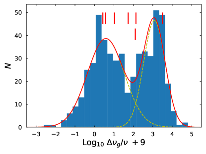
Figure 12: Distribution of relative pulsar glitch sizes according to the data in http://www.jb.man.ac.uk/pulsar/glitches.html, as given for August 2018. The solid line is the double-Gaussian best fit for the distribution; dashed lines show individual components. Vertical bars mark the positions of seven glitches of B1727 discussed in the text.

The small glitch peak is located around $\Delta\nu_{g}/\nu\approx 3\times 10^{-9}$ and the large glitch peak is near $10^{-6}$. The peaks are separated by a dip at $\Delta\nu_{\rm g}/\nu\sim 10^{-7}$. This distribution suggests that two different mechanisms may trigger small and large glitches. The cracking of the NS crust may be responsible for the small glitches, while other mechanisms, such as a critical superfluid vortex repining inside the star (e.g., “snowplough” glitch model) need to be invoked to explain large glitches as observed, i.e., in the Vela pulsar (Haskell & Melatos, 2015). Fractional sizes of the B1727 glitches are shown with the vertical bars in Figure 12. As seen, they do not follow the overall distribution. Three glitches of B1727 with $\Delta\nu_{\rm g}/\nu\approx 2.7,\,3.7,\,10.7\times 10^{-9}$ are compatible with the small glitch population, the largest recently discovered one clearly belongs to the large glitch population, while the rest three glitches with $\Delta\nu_{\rm g}/\nu\approx 54,\,126,\,136\times 10^{-9}$ fall exactly in the dip of the glitch distribution.

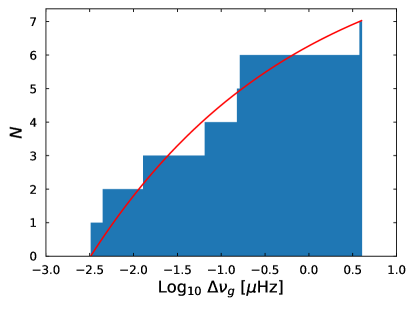
Figure 13: Cumulative distribution of the glitch sizes observed in B1727. The solid line shows the best-fit power law distribution.

Seven glitches detected in B1727 allows to roughly investigate the glitch statistics for this pulsar. In Figure 13, we show the cumulative distribution of glitch sizes (i.e. the number of glitches with $\Delta\nu_{g}$ smaller than the given one). The obtained broad distribution is similar to those for the Crab and similar pulsars (Espinoza et al., 2011) in contrast to Vela-like glitchers. The distribution in Figure 13 is well-fitted by the power-law (see, e.g., Melatos et al., 2008) with the index $\alpha=1.2\pm 0.3$ in agreement with the values found for other frequently glitching pulsars (Melatos et al., 2008; Haskell & Melatos, 2015). The best-fit power law is shown with the solid line in Figure 13. Figure 13 indicates that probably the same trigger mechanism operates in B1727, including the recent largest event. The glitch spin-up rate $\Delta\dot{\nu_{g}}$ for B1727 does not vary substantially from glitch to glitch and is consistent with what is typically observed for other pulsars of similar ages (Espinoza et al., 2011).

The exponential and fractional glitch recovery parameters $\tau_{d}$ and $Q$ were estimated only for three of seven B1727 glitches. The $Q$ histogram for all pulsars is also bimodal, pointing on two different mechanisms of the glitch recovery (Yu et al., 2013). The first peak is located near $Q\approx 0.01$ and the second is between 0.1 and 1. Interestingly, for all three glitches where $Q$ value was estimated, it falls in the dip between the two peaks of the distribution making it impossible to speculate about mechanisms of the glitch recoveries in B1727.

8 Conclusions

We measured, for the first time, the p.m. of the radio-bright pulsar B1727. Timing observations during 50 yr, since the pulsar discovery, and the interferometric positions for three epochs resulted in significant $\mu_{\alpha}=73\pm 15$ mas yr^-1 and $\mu_{\delta}=-132\pm 14$ mas yr^-1.

The obtained p.m. allowed us to reveal the birth place of B1727 near the center of the nearby evolved SNR RCW 114. This strongly suggests the genuine association between the pulsar and the SNR. The association enabled us to constrain self-consistently the properties of the system.

Based on the analysis of all the data, we argue that the system is located at $\approx 0.4-0.7$ kpc, much closer than given by the pulsar dispersion measure and current Galactic electron density maps. The dispersion measure distance results in unrealistically high transverse velocities of $\gtrsim 1900$ km s^-1. In contrast, the new distance and p.m. imply a reasonable pulsar transverse velocity of about 300–500 km s^-1. The inferred distance makes feasible B1727 parallax measurements with the VLBI which can help to set stronger constraints on the system parameters and to correct the electron density distribution towards the pulsar.

Based on the measured p.m. value and the pulsar shift from the remnant center, we conclude that the most plausible system age is about 50 kyr. For reasonable values of braking indices, this implies a relatively large pulsar initial period of about 0.5$-$0.6 s. Comparison of the RCW 114 data with the SNR evolution models shows that the remnant is at the middle of the PDS phase. The remnant properties are consistent with being a product of a usual neutrino-driven core-collapse supernovae. This places the system to the lower edge of the above distance range.

We detected two new glitches of the pulsar. Together with four glitches found previously and that of August 2017 this suggests a mean glitch rate for B1727 of 0.25 yr^-1. The pulsar likely demonstrates a broad range of the glitch sizes described by the power-law distribution.

Appendix A ATCA relative astrometry

Table 6: Reference sources used for the registration of the ATCA images.

Source #	R.A., J2000	Decl., J2000	$S/N$	$\chi^{2}_{11-16}$	$\chi^{2}_{11-16}$	$\chi^{2}_{11-05}$	$\chi^{2}_{11-05}$
				before	after	before	after
1	17h31m01$.\!\!^{\rm s}$385(15)	$-$47∘29′44$.\!\!^{\prime\prime}$37(22)	14	55	0.41	8.6	0.9
2	17h30m47$.\!\!^{\rm s}$294(10)	$-$47∘31′24$.\!\!^{\prime\prime}$78(15)	20	153	0.07	1.1	0.15
3	17h32m20$.\!\!^{\rm s}$880(16)	$-$47∘42′06$.\!\!^{\prime\prime}$04(24)	12	17	0.82	0.57	0.28
4	17h32m38$.\!\!^{\rm s}$665(12)	$-$47∘62′12$.\!\!^{\prime\prime}$03(17)	18	54	0.18	$\cdots$	$\cdots$
5	17h31m41$.\!\!^{\rm s}$379(7)	$-$47∘40′16$.\!\!^{\prime\prime}$59(10)	29	0.3	0.01	5.7	0.6
6	17h31m09$.\!\!^{\rm s}$344(31)	$-$47∘48′54$.\!\!^{\prime\prime}$89(47)	7	1.6	0.76	$\cdots$	$\cdots$
7	17h31m57$.\!\!^{\rm s}$777(9)	$-$47∘54′49$.\!\!^{\prime\prime}$68(13)	24	123	0.07	4.3	1.2
8	17h33m10$.\!\!^{\rm s}$537(10)	$-$47∘52′22$.\!\!^{\prime\prime}$49(14)	22	498	0.28	10.4	1.8

Note. — Source coordinates are given as measured on the 2011 image relative to the respective calibrator. $S/N$ is the source signal to noise ratio on the 2011 image. Four last columns show the weighted squared residuals ($\chi^{2}$) for individual sources for two image pairs before and after the registration; subscripts 11–16 and 11–05 denote the image pairs of 2011 and 2016, and of 2011 and 2005, respectively. Sources 4 and 6 were not detected firmly in the 2005 image and were not used.

Eight firmly detected point-like sources located in the pulsar vicinity were used for the relative astrometry of the ATCA images. Source positions on the 2011 image are listed in Table 6. This epoch is used as the reference. Two sources listed in Table 6 were not detected with the sufficient $S/N$ in the 2005 image. We define the discrepancy in the indiviual source positions on two images by means of $\chi^{2}$ as

$$\chi^{2}=\Delta x^{T}W^{-1}\Delta x,$$ (A1)

where $\Delta x=x_{2}-x_{1}$, $W=W_{1}+W_{2}$, and $(x_{i},W_{i}),\ i=1,2$ are source positions and their covariance matrices for two epochs 1 and 2. Then the initial $\chi^{2}$ summed over the sources is $\sum\chi^{2}_{11-05}=31$ for 12 dof (number of coordinates) for 2005–2011 astrometry and $\sum\chi^{2}_{11-05}=903$ for 16 dof for 2016–2011 astrometry. It is clear that the 2016 map differs substantially from the 2011 map. The same is true for the 2005 map, but to the less extent. Therefore we matched the 2005 and 2016 images to the 2011 image allowing for the coordinate transformation in the form

$$\mathbf{x}^{\prime}=a\hat{R}(\Theta)\left(\mathbf{x}+\delta\mathbf{x}\right),$$ (A2)

where $\mathbf{x}$ is the initial position in the image, $\mathbf{x}^{\prime}$ is the transformed position on the reference epoch, $\delta\mathbf{x}$ is the shift between maps, $\hat{R}(\Theta)$ is the rotation matrix which rotates the image by the angle $\Theta$, and $a$ is the scale parameter. The source positions on the 2011 epoch were fitted simultaneously with the transformation parameters, and, notably the pulsar position and proper motion. The pulsar positions here, however, were measured on the same images and using the same reference sources, i.e. in the off-pulse (unbinnned) mode in contrast to the positions used for the I solution in Section 4.

Table 7: Astrometric solution with respect to the 2011 image.

Epoch	$\delta x_{\alpha}$	$\delta x_{\delta}$	$\Theta$	$a-1$	$\chi^{2}_{\mathrm{tot}}$	$\chi^{2}_{\mathrm{tot}}$
	asec	asec	amin	$10^{-3}$	before	after
2005	$-0.59\pm 0.16$	$0.07\pm 0.15$	$-2.0\pm 0.5$	$2.1\pm 0.1$	31	5.7
2016	$0.03\pm 0.06$	$-0.56\pm 0.11$	$-0.2\pm 0.5$	$=a_{2005}$	903	2.6

Note. — $\delta x_{\alpha}$ and $\delta x_{\delta}$ are the image shifts in R.A. and decl. directions, respectively, $\Theta$ is the rotation angle, while the scale parameter $a$ is set the same for 2005$-$2011 and 2016$-$2011 registrations. Two last columns show the total $\chi^{2}$ before and after the registration (sums of the corresponding columns in Table 6).

Initially we performed registration allowing for the linear transformations only, i.e. setting $a=1$ in Equation (A2). Although sources’ offsets had generally reduced, there were still large differences in 2011–2016 positions (total discrepancy $\sum\chi^{2}_{11-16}=78.8$), while the 2005–2011 registration was formally good, with $\sum\chi^{2}_{11-05}=8.7$. These values and the visual inspection of the shifted source positions suggested that the linear transformation was not enough. Allowing the scale parameters to vary as well, we got a much better solution. Moreover, we found that the scale parameters for 2005 and 2016 epochs are comparable within uncertainties suggesting that it is actually the 2011 map that needs to be scaled. Therefore we performed the final registration tying the scale parameters for 2005–2011 and 2016–2011 registrations. The source registration becomes fairly good with $\sum\chi^{2}_{11-16}=2.6$ and $\sum\chi^{2}_{11-05}=5.7$ as indicated in Table 7 where the best-fit astrometric solution parameters are given. Examining these parameters we conclude that there is a significant (5$\sigma$) shift between the 2011 and 2016 images in decl. direction and the R.A. shift (at 3.7$\sigma$ level) between 2005 and 2011 images. In addition, the small rotation is preferrable between the 2005 and 2011 maps. The possible cause of the rotation can be due to one correlator cycle (10 s) timing mismatch between $uvw$ and visibiltities. The scale parameter $a=1.0021(1)$ is well-determined indicating that there is a problem in a 2011 image reconstruction. A possible cause of this systematics can be additional frequency averaging performed in the correlator control computer of CABB in the pulsar binning mode, a setup specific to the 2011 epoch. The pulsar proper motion determined in this solution is $\mu_{\alpha}=81\pm 19$ mas yr^-1 and $\mu_{\delta}=-132\pm 23$ mas yr^-1. We adopt these values as our ‘relative astrometry’ estimate in Sections 4–5. We also checked that the solution that completely neglects the rotation is slightly worse, but acceptable and results in the same p.m. parameters within errors.

References

- Astropy Collaboration et al. (2013) Astropy Collaboration, Robitaille, T. P., Tollerud, E. J., et al. 2013, A&A, 558, A33, doi: 10.1051/0004-6361/201322068
- Astropy Collaboration et al. (2018) Astropy Collaboration, Price-Whelan, A. M., Sipőcz, B. M., et al. 2018, AJ, 156, 123, doi: 10.3847/1538-3881/aabc4f
- Bailer-Jones et al. (2018) Bailer-Jones, C. A. L., Rybizki, J., Fouesneau, M., Mantelet, G., & Andrae, R. 2018, AJ, 156, 58, doi: 10.3847/1538-3881/aacb21
- Bedford et al. (1984) Bedford, D. K., Elliott, K. H., Ramsey, B., & Meaburn, J. 1984, MNRAS, 210, 693, doi: 10.1093/mnras/210.3.693
- Brisken et al. (2006) Brisken, W. F., Carrillo-Barragán, M., Kurtz, S., & Finley, J. P. 2006, ApJ, 652, 554, doi: 10.1086/507765
- Brisken et al. (2003) Brisken, W. F., Fruchter, A. S., Goss, W. M., Herrnstein, R. M., & Thorsett, S. E. 2003, AJ, 126, 3090, doi: 10.1086/379559
- Cappa de Nicolau et al. (1988) Cappa de Nicolau, C. E., Niemela, V. S., Dubner, G. M., & Arnal, E. M. 1988, AJ, 96, 1671, doi: 10.1086/114918
- Chatterjee et al. (2004) Chatterjee, S., Cordes, J. M., Vlemmings, W. H. T., et al. 2004, ApJ, 604, 339, doi: 10.1086/381748
- Cioffi et al. (1988) Cioffi, D. F., McKee, C. F., & Bertschinger, E. 1988, ApJ, 334, 252, doi: 10.1086/166834
- Coles et al. (2011) Coles, W., Hobbs, G., Champion, D. J., Manchester, R. N., & Verbiest, J. P. W. 2011, MNRAS, 418, 561, doi: 10.1111/j.1365-2966.2011.19505.x
- Condon et al. (1993) Condon, J. J., Griffith, M. R., & Wright, A. E. 1993, AJ, 106, 1095, doi: 10.1086/116707
- Cordes & Lazio (2002) Cordes, J. M., & Lazio, T. J. W. 2002, ArXiv Astrophysics e-prints
- D’Alessandro et al. (1993) D’Alessandro, F., McCulloch, P. M., King, E. A., Hamilton, P. A., & McConnell, D. 1993, MNRAS, 261, 883, doi: 10.1093/mnras/261.4.883
- De Luca (2017) De Luca, A. 2017, Journal of Physics: Conference Series, 932, 012006, doi: 10.1088/1742-6596/932/1/012006
- Deller et al. (2018) Deller, A. T., Goss, W. M., Brisken, W. F., et al. 2018, arXiv e-prints, arXiv:1808.09046. https://arxiv.org/abs/1808.09046
- Desvignes et al. (2016) Desvignes, G., Caballero, R. N., Lentati, L., et al. 2016, MNRAS, 458, 3341, doi: 10.1093/mnras/stw483
- Duncan et al. (1997) Duncan, A. R., Stewart, R. T., Haynes, R. F., & Jones, K. L. 1997, MNRAS, 287, 722, doi: 10.1093/mnras/287.4.722
- Edwards et al. (2006) Edwards, R. T., Hobbs, G. B., & Manchester, R. N. 2006, MNRAS, 372, 1549, doi: 10.1111/j.1365-2966.2006.10870.x
- Espinoza et al. (2011) Espinoza, C. M., Lyne, A. G., Stappers, B. W., & Kramer, M. 2011, MNRAS, 414, 1679, doi: 10.1111/j.1365-2966.2011.18503.x
- Faucher-Giguère & Kaspi (2006) Faucher-Giguère, C.-A., & Kaspi, V. M. 2006, ApJ, 643, 332, doi: 10.1086/501516
- Feroz et al. (2009) Feroz, F., Hobson, M. P., & Bridges, M. 2009, MNRAS, 398, 1601, doi: 10.1111/j.1365-2966.2009.14548.x
- Fesen et al. (1985) Fesen, R. A., Blair, W. P., & Kirshner, R. P. 1985, ApJ, 292, 29, doi: 10.1086/163130
- Gaensler & Johnston (1995) Gaensler, B. M., & Johnston, S. 1995, MNRAS, 277, 1243, doi: 10.1093/mnras/277.4.1243
- Gaustad et al. (2001) Gaustad, J. E., McCullough, P. R., Rosing, W., & Van Buren, D. 2001, PASP, 113, 1326, doi: 10.1086/323969
- Gooch (1996) Gooch, R. 1996, in Astronomical Society of the Pacific Conference Series, Vol. 101, Astronomical Data Analysis Software and Systems V, ed. G. H. Jacoby & J. Barnes, 80
- Gotthelf et al. (2013) Gotthelf, E. V., Halpern, J. P., & Alford, J. 2013, ApJ, 765, 58, doi: 10.1088/0004-637X/765/1/58
- Green (2014a) Green, D. A. 2014a, Bulletin of the Astronomical Society of India, 42, 47. https://arxiv.org/abs/1409.0637
- Green (2014b) —. 2014b, A Catalogue of Galactic Supernova Remnants (2014 May version), available at “http://www.mrao.cam.ac.uk/surveys/snrs/”
- Gvaramadze (2002) Gvaramadze, V. V. 2002, ArXiv Astrophysics e-prints
- Halpern & Gotthelf (2015) Halpern, J. P., & Gotthelf, E. V. 2015, ApJ, 812, 61, doi: 10.1088/0004-637X/812/1/61
- Haskell & Melatos (2015) Haskell, B., & Melatos, A. 2015, International Journal of Modern Physics D, 24, 1530008, doi: 10.1142/S0218271815300086
- Heger et al. (2003) Heger, A., Fryer, C. L., Woosley, S. E., Langer, N., & Hartmann, D. H. 2003, ApJ, 591, 288, doi: 10.1086/375341
- Hobbs et al. (2005) Hobbs, G., Lorimer, D. R., Lyne, A. G., & Kramer, M. 2005, MNRAS, 360, 974, doi: 10.1111/j.1365-2966.2005.09087.x
- Hobbs et al. (2006) Hobbs, G. B., Edwards, R. T., & Manchester, R. N. 2006, MNRAS, 369, 655, doi: 10.1111/j.1365-2966.2006.10302.x
- Hotan et al. (2004) Hotan, A. W., van Straten, W., & Manchester, R. N. 2004, PASA, 21, 302, doi: 10.1071/AS04022
- Hunter (2007) Hunter, J. D. 2007, Computing In Science & Engineering, 9, 90, doi: 10.1109/MCSE.2007.55
- Igoshev & Popov (2013) Igoshev, A. P., & Popov, S. B. 2013, MNRAS, 432, 967, doi: 10.1093/mnras/stt519
- Janka (2012) Janka, H.-T. 2012, Annual Review of Nuclear and Particle Science, 62, 407, doi: 10.1146/annurev-nucl-102711-094901
- Janka (2017) —. 2017, ApJ, 837, 84, doi: 10.3847/1538-4357/aa618e
- Jankowski et al. (2017) Jankowski, F., Bailes, M., Barr, E. D., et al. 2017, The Astronomer’s Telegram, 10770
- Jankowski et al. (2019) Jankowski, F., Bailes, M., van Straten, W., et al. 2019, MNRAS, 484, 3691, doi: 10.1093/mnras/sty3390
- Johnston et al. (1998) Johnston, S., Nicastro, L., & Koribalski, B. 1998, MNRAS, 297, 108, doi: 10.1046/j.1365-8711.1998.01461.x
- Jones et al. (2001–) Jones, E., Oliphant, T., Peterson, P., et al. 2001–, SciPy: Open source scientific tools for Python. http://www.scipy.org/
- Kalberla & Haud (2015) Kalberla, P. M. W., & Haud, U. 2015, A&A, 578, A78, doi: 10.1051/0004-6361/201525859
- Kaspi (1996) Kaspi, V. M. 1996, in Astronomical Society of the Pacific Conference Series, Vol. 105, IAU Colloq. 160: Pulsars: Problems and Progress, ed. S. Johnston, M. A. Walker, & M. Bailes, 375
- Kaspi et al. (1994) Kaspi, V. M., Manchester, R. N., Siegman, B., Johnston, S., & Lyne, A. G. 1994, ApJ, 422, L83, doi: 10.1086/187218
- Kim et al. (2010) Kim, I.-J., Min, K.-W., Seon, K.-I., Han, W., & Edelstein, J. 2010, ApJ, 709, 823, doi: 10.1088/0004-637X/709/2/823
- Kirichenko et al. (2015) Kirichenko, A., Shibanov, Y., Shternin, P., et al. 2015, MNRAS, 452, 3273, doi: 10.1093/mnras/stv1420
- Kirsten et al. (2015) Kirsten, F., Vlemmings, W., Campbell, R. M., Kramer, M., & Chatterjee, S. 2015, A&A, 577, A111, doi: 10.1051/0004-6361/201425562
- Large et al. (1968) Large, M. I., Vaughan, A. E., & Wielebinski, R. 1968, Nat, 220, 753, doi: 10.1038/220753a0
- Lentati et al. (2014) Lentati, L., Alexander, P., Hobson, M. P., et al. 2014, MNRAS, 437, 3004, doi: 10.1093/mnras/stt2122
- Li et al. (2016) Li, L., Wang, N., Yuan, J. P., et al. 2016, MNRAS, 460, 4011, doi: 10.1093/mnras/stw1262
- Lorimer & Kramer (2012) Lorimer, D. R., & Kramer, M. 2012, Handbook of Pulsar Astronomy (Cambridge, UK: Cambridge University Press)
- Manchester et al. (2005) Manchester, R. N., Hobbs, G. B., Teoh, A., & Hobbs, M. 2005, AJ, 129, 1993, doi: 10.1086/428488
- Manchester et al. (1983) Manchester, R. N., Newton, L. M., Goss, W. M., & Hamilton, P. A. 1983, MNRAS, 202, 269, doi: 10.1093/mnras/202.2.269
- Matthews et al. (1998) Matthews, B. C., Wallace, B. J., & Taylor, A. R. 1998, ApJ, 493, 312, doi: 10.1086/305112
- Meaburn et al. (1991) Meaburn, J., Goudis, C., Solomos, N., & Laspias, V. 1991, A&A, 252, 291
- Melatos et al. (2008) Melatos, A., Peralta, C., & Wyithe, J. S. B. 2008, ApJ, 672, 1103, doi: 10.1086/523349
- Müller (2017) Müller, B. 2017, in IAU Symposium, Vol. 329, The Lives and Death-Throes of Massive Stars, ed. J. J. Eldridge, J. C. Bray, L. A. S. McClelland, & L. Xiao, 17–24
- Müller et al. (2016) Müller, B., Heger, A., Liptai, D., & Cameron, J. B. 2016, MNRAS, 460, 742, doi: 10.1093/mnras/stw1083
- Müller et al. (2019) Müller, B., Tauris, T. M., Heger, A., et al. 2019, MNRAS, 484, 3307, doi: 10.1093/mnras/stz216
- Noutsos et al. (2013) Noutsos, A., Schnitzeler, D. H. F. M., Keane, E. F., Kramer, M., & Johnston, S. 2013, MNRAS, 430, 2281, doi: 10.1093/mnras/stt047
- Pejcha & Thompson (2015) Pejcha, O., & Thompson, T. A. 2015, ApJ, 801, 90, doi: 10.1088/0004-637X/801/2/90
- Popov & Turolla (2012) Popov, S. B., & Turolla, R. 2012, Ap&SS, 341, 457, doi: 10.1007/s10509-012-1100-z
- Ren et al. (2018) Ren, J.-J., Liu, X.-W., Chen, B.-Q., et al. 2018, Research in Astronomy and Astrophysics, 18, 111, doi: 10.1088/1674-4527/18/9/111
- Sault et al. (1995) Sault, R. J., Teuben, P. J., & Wright, M. C. H. 1995, in Astronomical Society of the Pacific Conference Series, Vol. 77, Astronomical Data Analysis Software and Systems IV, ed. R. A. Shaw, H. E. Payne, & J. J. E. Hayes, 433
- Shelton (1999) Shelton, R. L. 1999, ApJ, 521, 217, doi: 10.1086/307553
- Shternin et al. (2017) Shternin, P. S., Yu, M., Kirichenko, A. Y., et al. 2017, Journal of Physics : Conference Series, 932, 012004, doi: 10.1088/1742-6596/932/1/012004
- Smith et al. (2019) Smith, D. A., Bruel, P., Cognard, I., et al. 2019, ApJ, 871, 78, doi: 10.3847/1538-4357/aaf57d
- Sukhbold et al. (2016) Sukhbold, T., Ertl, T., Woosley, S. E., Brown, J. M., & Janka, H.-T. 2016, ApJ, 821, 38, doi: 10.3847/0004-637X/821/1/38
- Thorsett et al. (2003) Thorsett, S. E., Benjamin, R. A., Brisken, W. F., Golden, A., & Goss, W. M. 2003, ApJ, 592, L71, doi: 10.1086/377682
- Vaughan et al. (1974) Vaughan, A. E., Nicholson, M. J., & Disney, P. 1974, MNRAS, 168, 361, doi: 10.1093/mnras/168.2.361
- Verbunt et al. (2017) Verbunt, F., Igoshev, A., & Cator, E. 2017, A&A, 608, A57, doi: 10.1051/0004-6361/201731518
- Walker & Zealey (2001) Walker, A. J., & Zealey, W. J. 2001, MNRAS, 325, 287, doi: 10.1046/j.1365-8711.2001.04423.x
- Wang et al. (2000) Wang, N., Manchester, R. N., Pace, R. T., et al. 2000, MNRAS, 317, 843, doi: 10.1046/j.1365-8711.2000.03713.x
- Welsh et al. (2003) Welsh, B. Y., Sallmen, S., Jelinsky, S., & Lallement, R. 2003, A&A, 403, 605, doi: 10.1051/0004-6361:20030168
- Wilson et al. (2011) Wilson, W. E., Ferris, R. H., Axtens, P., et al. 2011, MNRAS, 416, 832, doi: 10.1111/j.1365-2966.2011.19054.x
- Wongwathanarat et al. (2013) Wongwathanarat, A., Janka, H. T., & Müller, E. 2013, A&A, 552, A126, doi: 10.1051/0004-6361/201220636
- Yao et al. (2017) Yao, J. M., Manchester, R. N., & Wang, N. 2017, ApJ, 835, 29, doi: 10.3847/1538-4357/835/1/29
- Yar-Uyaniker et al. (2004) Yar-Uyaniker, A., Uyaniker, B., & Kothes, R. 2004, ApJ, 616, 247, doi: 10.1086/424794
- Yu et al. (2013) Yu, M., Manchester, R. N., Hobbs, G., et al. 2013, MNRAS, 429, 688, doi: 10.1093/mnras/sts366