Ultra-diffuse galaxies in the Auriga simulations

Abstract

We investigate the formation of ultra-diffuse galaxies (UDGs) using the Auriga high-resolution cosmological magneto-hydrodynamical simulations of Milky Way-sized galaxies. We identify a sample of $92$ UDGs in the simulations that match a wide range of observables such as sizes, central surface brightness, Sérsic indices, colors, spatial distribution and abundance. Auriga UDGs have dynamical masses similar to normal dwarfs. In the field, the key to their origin is a strong correlation present in low-mass dark matter haloes between galaxy size and halo spin parameter. Field UDGs form in dark matter haloes with larger spins compared to normal dwarfs in the field, in agreement with previous semi-analytical models. Satellite UDGs, on the other hand, have two different origins: $\sim 55\%$ of them formed as field UDGs before they were accreted; the remaining $\sim 45\%$ were normal field dwarfs that subsequently turned into UDGs as a result of tidal interactions.

1 Introduction

Ultra-diffuse galaxies (hereafter UDGs) are “extreme” galaxies whose sizes are as large as $L_{\star}$ galaxies but whose luminosities are as faint as dwarf galaxies. Specifically, UDGs are usually defined as galaxies with $g$-band central surface brightnesses, $\mu_{g}(0)\ga 24$ $\mathrm{mag}$ $\mathrm{arcsec}^{-2}$ and effective radii, $r_{\mathrm{e}}\ga 1.5$ $\mathrm{kpc}$ (van Dokkum et al., 2015). While such low surface brightness galaxies have been known since 1980s (e.g. Impey et al., 1988; Dalcanton et al., 1997), a survey of $47$ UDGs in the Coma cluster presented by van Dokkum et al. (2015) has unveiled their ubiquity, and drawn much attention recently.

After the work of van Dokkum et al. (2015), further observations of UDGs in different environments, from dense to sparse, have been reported in:

(i) Clusters such as Coma (Koda et al., 2015; Yagi et al., 2016; Ruiz-Lara et al., 2018), Virgo (Mihos et al., 2015; Beasley et al., 2016; Mihos et al., 2017; Toloba et al., 2018), Fornax (Muñoz et al., 2015; Venhola et al., 2017); 8 clusters in the redshift range of $0.044<z<0.063$ (van der Burg et al., 2016) and another 10 clusters with $z\leq 0.09$ (Sifón et al., 2018); Abell 168 (Román & Trujillo, 2017a); Abell 2744 (Janssens et al., 2017; Lee et al., 2017); Abell S1063 (Lee et al., 2017); Pegasus I and Pegasus II (Shi et al., 2017); and Perseus (Wittmann et al., 2017).

(ii) Groups such as NGC 3414 and NGC 5371 (Makarov et al., 2015), Centaurus A (Crnojević et al., 2016), NGC 253 (Toloba et al., 2016), NGC 5473/5485 (Merritt et al., 2016), HCG44 (Smith Castelli et al., 2016), HCG07, HCG25 and HCG98 (Román & Trujillo, 2017b), M77 (Trujillo et al., 2017); 325 groups in KiDs and GAMA surveys (van der Burg et al., 2017); HCG95 (Shi et al., 2017); NGC 4958, M81 and the Local Volume (Karachentsev et al., 2017); Leo-I (Müller et al., 2018); NGC 1052 (van Dokkum et al., 2018a; Cohen et al., 2018); and M96 (Cohen et al., 2018).

(iii) Filaments and the field, such as DGSAT I in the filament of the Pisces-Perseus supercluster (Martínez-Delgado et al., 2016); filaments and the field around Abell 168 (Román & Trujillo, 2017a); SECCO-dI-1 and SECCO-dI-2 (Bellazzini et al., 2017); DF03 which was originally cataloged by van Dokkum et al. (2015) and later shown to be a field UDG with spectroscopy by Kadowaki, Zaritsky & Donnerstein (2017); 115 isolated UDGs from the ALFALFA survey (Leisman et al., 2017); Yagi771, which was originally cataloged by Yagi et al. (2016) and later shown to be a field UDG by Alabi et al. (2018); R-127-1 and M-161-1 (Papastergis et al., 2017), etc. See also Yagi et al. (2016) for a search of UDGs in previous literatures.

From the observations above, it is found that UDGs in clusters tend to be red, dark matter-dominated, have Sérsic indices slightly smaller than $1$ (e.g. van Dokkum et al., 2015; Koda et al., 2015; Román & Trujillo, 2017a), possibly have a relatively higher specific frequency of globular clusters than other typical dwarfs at similar luminosities (e.g. van Dokkum et al., 2017; Lim et al., 2018; Amorisco et al., 2018), and their stellar populations tend to be old and metal-poor (e.g. Kadowaki et al., 2017; Ferré-Mateu et al., 2018; Gu et al., 2018; Pandya et al., 2018; Ruiz-Lara et al., 2018). Furthermore, unlike typical dwarfs, UDGs tend to be absent in the centre of clusters (e.g. van Dokkum et al., 2015; van der Burg et al., 2016). The number of UDGs in a cluster is found to be approximately proportional to the host halo mass (van der Burg et al., 2016). In contrast, UDGs in lower density environments tend to be bluer, more irregular, and some of them are gas rich (e.g. Bellazzini et al., 2017; Leisman et al., 2017; Papastergis et al., 2017; Román & Trujillo, 2017b). They might have younger and more metal-rich stellar populations than their cluster counterparts (see Pandya et al., 2018, for the example of DGSAT 1).

Given the ubiquity of these low surface brightness objects, a natural question arises: how do UDGs form? Three possible origins have been proposed: (i) failed $L_{\star}$ galaxies which have dark matter haloes with masses of $\sim 10^{12}$ ${\rm M}_{\odot}$ and lost their gas due to some physical process after forming its first generation of stars at high redshift (see e.g. van Dokkum et al., 2015; van Dokkum et al., 2016; Toloba et al., 2018), (ii) genuine dwarfs (halo masses $\la 10^{11}$ ${\rm M}_{\odot}$) whose extended sizes are driven by their high spins (see e.g. Amorisco & Loeb, 2016; Leisman et al., 2017; Rong et al., 2017; Spekkens & Karunakaran, 2018) or feedback outflows (Di Cintio et al., 2017; Chan et al., 2018), and (iii) tidal galaxies (e.g. Venhola et al., 2017; Carleton et al., 2019; Toloba et al., 2018).

To distinguish between the scenarios of failed $L_{\star}$ galaxies and genuine dwarfs, a useful probe are the galaxies’ virial masses. Several methods have been used to determine virial masses of UDGs, for example, stellar kinematics from spectroscopy (van Dokkum et al., 2016, 2017), dynamics of globular clusters (Beasley et al., 2016; van Dokkum et al., 2018a), specific frequency of globular clusters (Beasley et al., 2016; Beasley & Trujillo, 2016; Peng & Lim, 2016; van Dokkum et al., 2017; Amorisco et al., 2018; Lim et al., 2018; Toloba et al., 2018), galaxy scaling relations (Lee et al., 2017; Zaritsky, 2017), HI rotation curves (Leisman et al., 2017), width of HI lines (Trujillo et al., 2017), and weak gravitational lensing (Sifón et al., 2018). From these observations, van Dokkum et al. (2016) show that one UDG in the Coma cluster, DF 44, has a virial mass of $M_{200}\sim 10^{12}$ ${\rm M}_{\odot}$, and Toloba et al. (2018) show that two UDGs in the Virgo cluster, VLSB-B and VCC615, are consistent with $\sim 10^{12}$ ${\rm M}_{\odot}$ dark matter haloes. Their results support the scenario of failed $L_{\star}$ galaxies. On the other hand, many other studies suggest UDG virial masses similar to those of dwarf galaxies (see e.g. Beasley et al., 2016; Beasley & Trujillo, 2016; Peng & Lim, 2016; Amorisco et al., 2018). There are also studies showing that the virial masses of UDGs range from dwarfs to $L_{\star}$ galaxies, and thus hint at more than one formation mechanism (e.g. Zaritsky, 2017; Sifón et al., 2018).

While most of UDGs do not show tidal features (see e.g. van Dokkum et al., 2015; Mowla et al., 2017), there are some, both in high and low density environments, that are observed to be experiencing tidal effects, supporting the view that at least some UDGs may originate from the third mechanism. Examples of UDGs which may be associated with tidal origins can be found in Mihos et al. (2015); Crnojević et al. (2016); Merritt et al. (2016); Toloba et al. (2016); Venhola et al. (2017); Wittmann et al. (2017); Greco et al. (2018); Toloba et al. (2018).

There is still no consensus regarding the formation of UDGs, and as we discussed, there are hints that UDGs may have multiple origins. More observational and theoretical work is necessary to solve this mystery. Among different approaches to exploring UDGs, numerical simulations are one of the most useful, because they allow us to trace the entire evolutionary paths of galaxies. However, up to now, there are still few works on simulated UDGs. Yozin & Bekki (2015) used idealize hydrodynamical simulations to consider possible evolutionary histories for the Coma UDGs. They show that the red UDGs in the Coma cluster are possibly galaxies which are accreted into the cluster at $z\sim 2$, and then efficiently quenched by ram pressure stripping during the first infall, thus becoming red. Based on the Millennium-II (Boylan-Kolchin et al., 2009) and Phoenix (Gao et al., 2012) dark matter simulations and the semi-analytical model of Guo et al. (2011), Rong et al. (2017) show that UDGs are genuine dwarf galaxies whose spatially extended sizes are due to the combination of the late formation time and high spins of their host haloes.

Di Cintio et al. (2017) used zoom-in cosmological hydrodynamical simulations of isolated galaxies, the NIHAO simulations (Wang et al., 2015a), to address the origin of UDGs. They identify $21$ UDGs from their simulations with definitions slightly different from observations, and show that these UDGs, which live in dwarf-sized dark matter haloes with typical spins, originate from supernovae feedback driving gas outflows. Jiang et al. (2019) further looked at UDGs using a zoom-in hydrodynamical simulation of a group galaxy, and show that the satellite UDGs in the group galaxy are either from the infall feedback-driven field UDGs or form by tidal puffing up and ram-pressure stripping. With $6$ isolated dwarf galaxies from the FIRE-2 zoom-in hydrodynamical simulations (Hopkins et al., 2018), Chan et al. (2018) support the feedback outflow scenario. They further mimic the quenching effects in cluster environments by artificially stopping star formation in a galaxy at a certain redshift and passively evolving its stellar population to $z=0$, and show that quenching processes can reproduce the observed properties of UDGs in the Coma cluster. Note that the UDG sample sizes of the NIHAO and FIRE simulations are quite limited, and comparing to the normal dwarfs in the same mass bin, these simulations may produce over abundant UDGs; see their Fig. 1 and related discussions in Jiang et al. (2019).

Given that the feedback outflow mechanism proposed in the NIHAO and FIRE simulations is different from the high-spin mechanism suggested by semi-analytical models, and we still do not have consensus on the detailed implementations and parameters for the subgrid models in hydrodynamical simulations, in the current stage, studying UDGs with different and independent simulations is necessary. This motivates us to use a set of high-resolution zoom-in simulations, the Auriga simulation (Grand et al., 2017), to study the formation and evolution of UDGs. The Auriga simulations are a set of zoom-in simulations of isolated Milky Way-sized galaxies using a state-of-the-art hydrodynamical code. The typical baryonic particle mass of the Auriga simulations is $m_{b}=5\times 10^{4}$ ${\rm M}_{\odot}$, which should be sufficient to study UDGs with stellar masses $\sim 10^{8}$ ${\rm M}_{\odot}$. The sample of $30$ Milky Way-sized galaxies also makes the Auriga simulations a good choice to study simulated UDGs in a statistical way.

The organization of this paper is as follows. In Section 2, we describe the simulation details and the procedures to identify simulated UDGs. In Section 3, we compare the properties of simulated UDGs to those from observations. Then we investigate the formation mechanisms of UDGs in Section 4. Our conclusions are presented in Section 5.

2 Methodology

2.1 Simulations

The Auriga simulations are a suite of $30$ cosmological magneto-hydrodynamical zoom-in simulations of isolated Milky Way-sized galaxies and their surroundings. These simulations are denoted by ‘Au-$N$’ with $N$ varying from $1$ to $30$ in this study. The parent dark matter haloes of the Auriga zoom-in galaxies were selected from a dark matter-only EAGLE simulation (Schaye et al., 2015). The simulations were performed with the $N$-body + magneto-hydrodynamical moving mesh code Arepo (Springel, 2010). The subgrid physics models are detailed in Grand et al. (2017). The adopted cosmological parameters are $\Omega_{m}=0.307$, $\Omega_{b}=0.048$, $\Omega_{\Lambda}=0.693$, and $h=0.6777$ (Planck Collaboration et al., 2014). The typical masses for high-resolution dark matter and star particles are $m_{\mathrm{DM}}=3\times 10^{5}$ ${\rm M}_{\odot}$ and $m_{\mathrm{b}}=5\times 10^{4}$ ${\rm M}_{\odot}$, respectively. Before $z=1$, the comoving softening length for high-resolution dark matter and star particles is $\epsilon=500$ $h^{-1}\mathrm{pc}$. After $z=1$, the simulations adopt a fixed physical softening length of $\epsilon=369$ $\mathrm{pc}$. Groups were identified with the friends-of-friends algorithm (Davis et al., 1985), and subhaloes were further extracted with the SUBFIND algorithm (Springel et al., 2001). To trace the growth histories of subhaloes, merger trees were constructed with the LHaloTree algorithm described in Springel et al. (2005). The Auriga simulations successfully reproduce a range of observables of our Milky Way Galaxy, for example, stellar masses, disc sizes, rotation curves, star formation rates, and metallicities (Grand et al., 2017), and its satellites (Simpson et al., 2018).

2.2 UDG sample

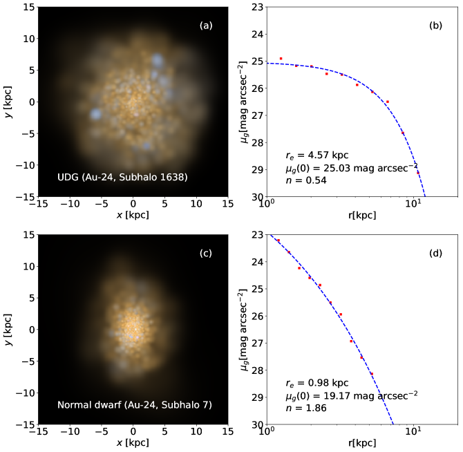
Figure 1: Face-on projected stellar densities and fitted projected surface brightness profiles for a UDG (upper panels) and a normal dwarf (lower panels) in the Auriga simulations. The RGB images on the left column are synthesized from the $i$-, $r$-, and $g$-band luminosities of star particles. The subhalo IDs are the indices from the SUBFIND subhalo catalog. In the right panels, the red squares show the projected surface brightness profiles computed from the simulations, and the blue dashed lines give the fitted Sérsic profiles. The best-fit $r_{e}$, $\mu_{g}(0)$ and $n$ are summarized in the corresponding panels. Note that these two galaxies have similar stellar mass (the stellar masses within $2r_{\star,1/2}$ for the UDG and the normal dwarf are $2.14\times 10^{8}$ ${\rm M}_{\odot}$ and $2.37\times 10^{8}$ ${\rm M}_{\odot}$, respectively), but very different appearance.

To identify UDGs in the Auriga simulations, we applied the following method:

(i) Rotate the subhalo (galaxy) with more than $500$ star particles to the face-on direction. We compute the inertia tensor for the star particles within two times the half stellar mass radius ($r_{\star,1/2}$) of the galaxy,

$$\mathcal{I}_{\alpha\beta}=\sum_{i}m_{i}(x_{i,\alpha}-x_{c,\alpha})(x_{i,\beta}-x_{c,\beta}),$$ (1)

where $m_{i}$ is the mass of the $i$-th star particle, $x_{i,\alpha}$ is the $\alpha$-th component of the $i$-th particle’s coordinate, and $x_{c,\alpha}$ is the $\alpha$-th component of the galaxy’s center coordinate. The line-of-sight direction is defined as the eigenvector corresponding to the smallest eigenvalue of $\mathcal{I}_{\alpha\beta}$. All the star particles are then projected onto the face-on plane.

(ii) Compute the $g$-band projected surface brightness profile $I_{g}(r)$. We calculate the circular $I_{g}(r)$ in the range $[3\epsilon,3r_{\star,1/2}]$ with $N_{\mathrm{bin}}=10$ equal logarithmic bins. In each bin, we compute the sum of the $g$-band fluxes of all star particles within this radial bin, $F_{g}(r_{i})$, and the area of the ring, $A_{i}=\pi(r_{i,R}^{2}-r_{i,L}^{2})$, with $r_{i,L}$ and $r_{i,R}$ being the inner and outer radius of the $i$-th bin respectively. Then the surface brightness at this bin is:

$$I_{g}(r_{i})=F_{g}(r_{i})/A_{i}.$$ (2)

We have varied the radial range (e.g. $[3\epsilon,2r_{\star,1/2}]$) and the number of bins (e.g. from 8 to 12), and found that this has negligible effect on the results.

(iii) Fit $I_{g}(r)$ with a Sérsic profile,

$$I_{g}(r)=I_{e}\exp\left\{-b_{n}\left[\left(\frac{r}{r_{e}}\right)^{1/n}-1\right]\right\},$$ (3)

where $I_{e}$, $r_{e}$ and $n$ are free parameters; $b_{n}$ satisfies $\gamma(2n,b_{n})=\Gamma(2n)/2$, where $\Gamma(x)$ and $\gamma(s,x)$ are the Gamma and lower incomplete Gamma functions. The best fit is obtained by minimizing the dimensionless figure-of-merit function (Navarro et al., 2010)

$$Q^{2}=\frac{1}{N_{\mathrm{bin}}}\sum^{N_{\mathrm{bin}}}_{i=1}\left(\log I_{i}^{\mathrm{data}}-\log I_{i}^{\mathrm{model}}\right)^{2}.$$ (4)

Once we obtain the fitted Sérsic profile, the central surface brightness, $\mu_{g}(0)$, can be obtained by expressing $I_{g}(0)$ in units of $\mathrm{mag}$ $\mathrm{arcsec}^{-2}$. AB magnitudes are adopted here. Note that some galaxies are poorly fitted with a Sérsic profile, and thus we only use galaxies with good fits ($Q^{2}<0.05$) and with $n\leq 4$ to define UDGs in this study. See Panels (b) and (d) of Fig. 1 for the projected surface brightness profiles and the fits for two example galaxies.

(iv) Following the definition in the observations (e.g. van Dokkum et al., 2015), we define the Auriga galaxies with $\mu_{g}(0)\geq 24$ $\mathrm{mag}$ $\mathrm{arcsec}^{-2}$, $r_{e}\geq 1.5$ $\mathrm{kpc}$ and $-18\leq M_{g}\leq-12$ as UDGs. $M_{g}$ here denotes the absolute $g$-band magnitude of the galaxy. For comparison, we also define a sample of normal dwarfs from the remaining non-UDGs. The normal dwarfs consist of galaxies which can be fitted with a Sérsic profile (with $n\leq 4$) and are in the same $g$-band magnitude range as UDGs.

Note that we only consider Auriga UDGs and normal dwarfs with more than $500$ star particles. When fitting the profiles, we also require each radial bin to contain at least $10$ particles. To avoid possible contamination from particles in the lower resolution region of the simulations, we only consider those galaxies whose distances to the central Milky Way-sized host satisfy $d<1$ $h^{-1}\mathrm{Mpc}$, and we further exclude galaxies which contain low-resolution particles within radius $10r_{1/2}$, which roughly equals three times the virial radius assuming an NFW density profile. Here $r_{1/2}$ is the subhalo half total mass radius.

The numbers of UDGs, non-UDGs and selected normal dwarfs in our sample are summarized in Table 1. Note that none of the thirty central galaxies in the Auriga simulations are classified as UDG according to the above definitions. In total, we identify $92$ UDGs from $30$ Auriga simulations, $38$ of which are satellites (i.e. galaxies inside the virial radius of the host galaxy, $d\leq R_{200}$), while the remaining $54$ UDGs are in the field (i.e. $R_{200}<d<1$ $h^{-1}\mathrm{Mpc}$). In Fig. 1, we illustrate examples of a UDG and a normal dwarf galaxy which have similar stellar mass. Clearly the UDG has a very extended and diffuse appearance, while the normal dwarf looks more compact and brighter in the center.

Apart from the thirty simulations (‘Level-4’) mentioned above, the Auriga project has an additional six simulations (‘Level-3’) with eight times better mass resolution. We have also identified UDGs in the Level-3 simulations, and found that the UDG properties from Level-4 converge well to those of Level-3 (see Appendix A for details). In this study, we analyze the Level-4 simulations in order to have better statistics.

Table 1: Number of galaxies in the sample. Non-UDGs consist of all galaxies (including both galaxies with and without successful Sérsic fits) which are not defined as UDGs in the simulations (except the central Milky Way-sized host galaxies).

Galaxies $(M_{g}\leq-12)$	$d\leq R_{200}$	$d<1$ $h^{-1}\mathrm{Mpc}$
UDGs	$38$	$92$
Non-UDGs	$89$	$358$
Normal dwarfs selected from non-UDGs	$48$	$173$

3 General properties

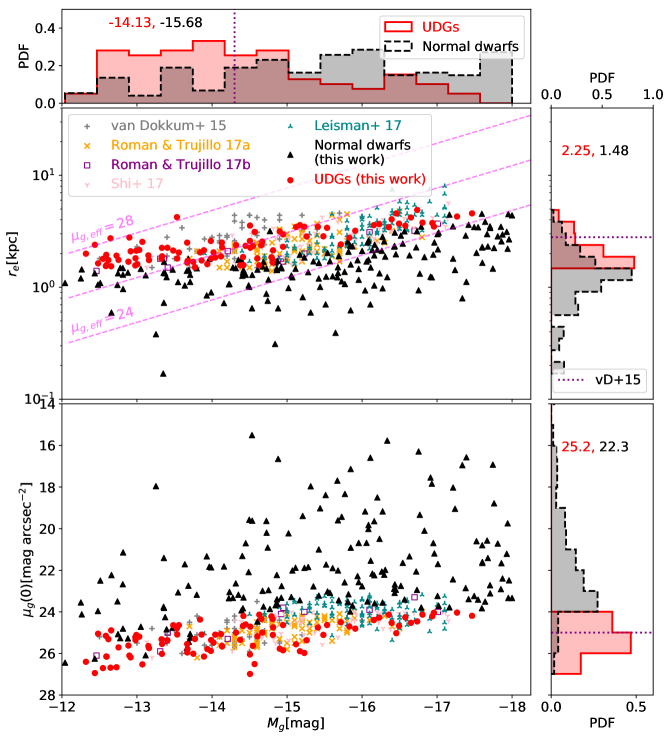
Figure 2: Relations between effective radius and central surface brightness, and $g$-band magnitude for Auriga galaxies. UDGs and normal dwarfs from Auriga are plotted as red circles and black triangles respectively. As a comparison, we also plot observed UDGs in different environments, i.e., the Coma cluster (van Dokkum et al., 2015), the Abell 168 cluster and its surrounding groups and filaments (Román & Trujillo, 2017a), groups (Román & Trujillo, 2017b; Shi et al., 2017) and the field (Leisman et al., 2017). The colors and symbols indicating different observed UDGs are given in the legend of the upper panel. The magenta dashed lines present the size-magnitude relations for different effective surface brightness, i.e., $\mu_{g,\mathrm{eff}}=28,26,24$ $\mathrm{mag}$ $\mathrm{arcsec}^{-2}$ (from top to bottom). We also plot the probability distribution functions (PDFs) of $M_{g}$, $r_{e}$ and $\mu_{g}(0)$ for UDGs (red solid) and normal dwarfs (black dashed). The first number in each histogram panel gives the median value for UDGs and the second for normal dwarfs. The purple dotted lines mark the median values from the Coma UDGs in van Dokkum et al. (2015).

In this section, we compare the general properties of UDGs in the Auriga simulations and observations. We first show the size - magnitude and central surface brightness - magnitude distributions of the Auriga UDGs as red circles in Fig. 2. In the same figure, we also show the same distribution for the Auriga normal dwarfs with black triangles, together with observed UDGs from different environments. From the plot, we see that the Auriga simulations reproduce well the observed size-magnitude and central surface brightness-magnitude relations for UDGs. As a quantitative comparison, we also plot the probability distribution functions (PDFs) of $M_{g}$, $r_{e}$, and $\mu_{g}(0)$, and compare their median values with those from the Coma UDGs in van Dokkum et al. (2015) (the dotted lines). The UDGs in the Auriga simulations (the Coma cluster) have a median absolute $g$-band magnitude $\langle M_{g}\rangle=-14.1$ $(-14.3)$, a median effective radius $\langle r_{e}\rangle=2.3$ $(2.8)$ kpc, and a median central surface brightness $\langle\mu_{g}(0)\rangle=25.2$ $(25.0)$ mag arcsec^-2, in broad agreement with observations.

We also see that Auriga UDGs and normal dwarfs form a continuous distribution in the size (or central surface brightness) - magnitude plane. This is a hint that UDGs are not a distinct population from normal dwarfs but merely the “extreme” galaxies in the same luminosity range (see Danieli & van Dokkum, 2019, for a similar result for galaxies in the Coma cluster).

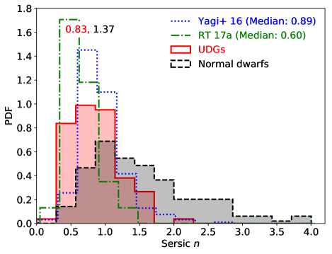
Figure 3: Sérsic indices of UDGs (red solid) and normal dwarfs (black dashed) in the Auriga simulations. The first number in the upper left corner gives the median value for UDGs and the second for normal dwarfs. We also plot the observational data from Yagi et al. (2016) (blue dotted) and Román & Trujillo (2017a) (green dash-dotted), and their median values are given in parentheses. Specifically, the plotted $328$ UDGs from Yagi et al. (2016) are those with $r_{e}>1.5$ kpc and “better-fitted” model flag $\neq 0$ in the catalog, and their $n$ comes from a single Sérsic fitting or a PSF+Sérsic fitting according to the better-fitted model flag.

The distribution of Sérsic index for the Auriga UDGs is shown in Fig. 3, where we also plot the distributions of observed UDGs derived by Yagi et al. (2016) and Román & Trujillo (2017a) for comparison. Our UDG sample tends to have $n$ smaller than $1$ (with a median of $0.83$), which is consistent with the observational results. At the same time, our normal dwarfs tend to have a larger $n$, with a median of $1.37$.

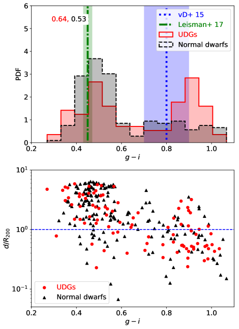
Figure 4: Top: color distributions of Auriga UDGs and normal dwarfs. The first number in the upper left corner gives the median for UDGs and the second for normal dwarfs. The blue dotted line and the corresponding shaded region show the mean and scatter of the cluster UDG sample from van Dokkum et al. (2015), while the green dash-dotted ones give those of field UDGs from Leisman et al. (2017). Bottom: relation between galaxy color and distance to the host galaxy. The blue dashed line marks the virial radius of the host haloes.

The $g-i$ color distribution for Auriga UDGs is presented in the upper panel of Fig. 4. Interestingly, the distribution of $g-i$ for UDGs is clearly bimodal. In the observations, red UDGs are usually found in high density environments (e.g. in the Coma cluster as reported in van Dokkum et al., 2015), while bluer UDGs are observed in the field (e.g. Leisman et al., 2017). We also show the mean and scatter of UDGs in clusters and the field from observations in Fig. 4; our simulated UDGs show fairly similar colors to these two samples. If we look at the relation between a galaxy’s distance to the host galaxy and its color, which is shown in the lower panel of Fig. 4, we can readily find that the blue UDGs in our sample tend to reside in the field ($d/R_{200}>1$), while the red ones tend to be satellites ($d/R_{200}<1$). But there is also a small fraction of blue UDGs inside the host’s $R_{200}$. We have traced their evolution histories with merger trees, and found that most of these blue galaxies are newly accreted systems. Similarly, there is a small fraction of red UDGs in the field, and they are usually ‘backsplash’ galaxies, i.e. galaxies that crossed $R_{200}$ at an earlier time but became field galaxies again at $z=0$. Such backsplash galaxies were quenched during their earlier infall; see Simpson et al. (2018) for a detailed investigations. Overall, the normal dwarfs share a similar color distribution and distance - color relation as UDGs. They tend to have a higher fraction of blue colors; this is simply because there are more normal dwarfs than UDGs in our sample of field objects (see Table 1).

From the lower panel of Fig. 4, we can also notice that no UDGs reside within $0.2R_{200}$, while some normal dwarfs can survive further in (e.g. $d<0.1R_{200}$). This is similar to the observed UDGs in clusters. For example, van Dokkum et al. (2015) find no UDGs within the central $\sim 300$ kpc ($\sim 0.11R_{200}$ assuming $R_{200}\approx 2.8$ Mpc for the Coma cluster; see Kubo et al., 2007) region in the Coma cluster; van der Burg et al. (2016) show that a model without UDGs in the central $0.15R_{200}$ region is consistent with their observed radial distribution of UDGs for 8 nearby clusters (see Mancera Piña et al., 2018, for a similar result).

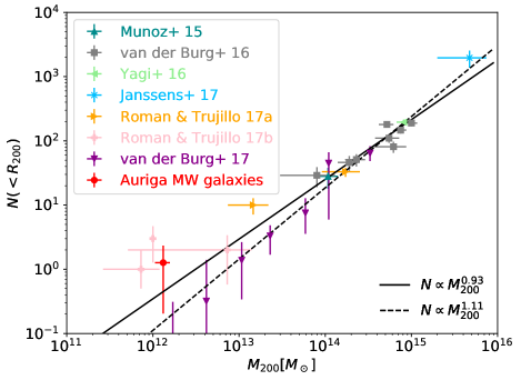
Figure 5: Relation between the number of satellite UDGs and host halo mass. The red dot with error bars (at $M_{200}=(1.32\pm 0.26)\times 10^{12}$ ${\rm M}_{\odot}$ and $N=1.27\pm 1.06$) marks the results for Auriga host galaxies, while other data points come from different observations as indicated in the legend. The solid and dashed lines show the power-law relations $N\propto M_{200}^{0.93}$ from Janssens et al. (2017) and $N\propto M_{200}^{1.11}$ from van der Burg et al. (2017), respectively.

In the observations, it was found that the number of satellite UDGs is approximately proportional to the host halo mass (e.g. van der Burg et al., 2016). In the Auriga simulations, we find that there are on average $1.27\pm 1.06$ satellite UDGs in a Milky Way-sized galaxy. In Fig. 5, we plot the Auriga UDGs in the number of satellite UDGs - host halo mass plane, together with data collected from observations. The abundance of Auriga satellite UDGs is consistent with those from observations. It approximately follows the power law relation inferred from observations, $N\propto M_{200}^{0.93\pm 0.16}$ (Janssens et al., 2017). The Auriga prediction is especially close to the results from Román & Trujillo (2017b). However, we should also note that there is still a relatively large scatter in the observed abundance of UDGs in Milky Way-sized galaxies. For example, van der Burg et al. (2017) find fewer UDGs in galaxies with similar halo masses, and they thus find a steeper power-law relation, $N\propto M_{200}^{1.11\pm 0.07}$.

There are claims in the literature that the Milky Way Galaxy has one satellite UDG, the Sagittarius dSph, and that the Andromeda galaxy has two satellite UDGs, And XIX and Cas III (see e.g. Yagi et al., 2016; Karachentsev et al., 2017; Rong et al., 2017). This is consistent with our predictions on the abundance of satellite UDGs in Milky Way-sized galaxies.

Given that the Auriga UDGs are similar to the observed UDGs in size, central surface brightness, Sérsic index, color, spatial distribution and abundance, we conclude that the Auriga simulations successfully reproduce the observed UDGs. Therefore, it becomes viable for us to use the Auriga simulations to further study their origin which is the main topic of the remainder of this paper. From the comparisons between simulated UDGs and normal dwarfs, we can find that, apart from being more extended and fainter, UDGs are quite similar to normal dwarfs in many aspects. This suggests that UDGs may just be genuine dwarfs, rather than a distinct population. We will explore the dwarf nature of UDGs in more detail in the next section.

Note that the properties of the Auriga UDGs presented in this section can also be regarded as the predictions for UDGs in/around Milky Way-sized galaxies. For example, one of the predictions is that blue and red UDGs have roughly equal numbers within the spherical region with a radius of $\sim 1$ $h^{-1}{\rm Mpc}$ around a Milky Way-sized galaxy. It will be interesting to test this prediction with future observations.

4 Formation of UDGs

4.1 Halo masses, spins, and morphology

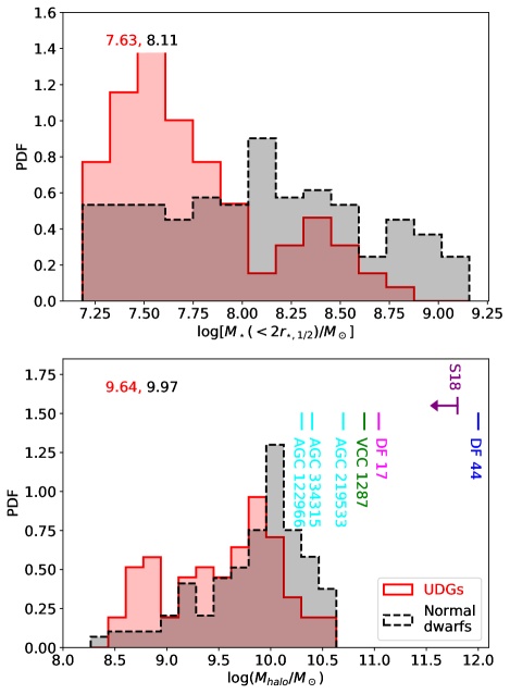
Figure 6: Top: distribution of stellar masses for UDGs (red solid) and normal dwarfs (black dashed). The first (second) number in the upper left corner gives the median for UDGs (normal dwarfs). Bottom: distribution of halo masses for UDGs and normal dwarfs. The halo masses of several observed UDGs are also indicated: DF 44 (van Dokkum et al., 2016), DF 17 (Beasley & Trujillo, 2016; Peng & Lim, 2016), and VCC 1287 (Beasley et al., 2016) in clusters, and AGC 219533, 334315, 122966 (Leisman et al., 2017) in the field. The line segment and the arrow labelled with “S18” mark the upper limit of halo masses for 784 UDGs in 18 clusters estimated by Sifón et al. (2018) with weak gravitational lensing.

A key quantity to consider when distinguishing between the scenarios of failed $L_{\star}$ galaxies and genuine dwarf galaxies is the dynamical mass of UDGs. In Fig. 6, we plot the distributions of the stellar masses of the UDGs measured within twice the half stellar mass radius, $M_{\star}(<2r_{\star,1/2})$, and their total subhalo masses, $M_{\mathrm{halo}}$ (i.e. the total mass of the particles and cells that are bound to the subhalo). Our simulated UDGs have a median stellar mass similar to normal dwarfs, $\langle M_{\star}\rangle=4.3\times 10^{7}{\rm M}_{\odot}$. Also, the Auriga UDGs have a median total subhalo mass of $\langle M_{\mathrm{halo}}\rangle=4.4\times 10^{9}$ ${\rm M}_{\odot}$ and a maximum of $3.1\times 10^{10}$ ${\rm M}_{\odot}$. This suggests that all Auriga UDGs are genuine galaxies with dwarf halo masses, not failed $L_{\star}$ galaxies. In Fig. 6 we also plot the halo masses of several observed UDGs. The Auriga UDGs tend to have total masses smaller than those of observed cluster UDGs (e.g. DF 44, DF 17, VCC 1287, and the mass upper limit inferred from $784$ cluster UDGs), but have total masses similar to field UDGs (e.g. the three UDGs from Leisman et al., 2017). This hints at a possible dependence of UDGs dynamical masses on their host galaxy environments.

Having confirmed that Auriga UDGs are genuine dwarf galaxies, the question arises of why are they more extended than normal dwarfs. As suggested by semi-analytical models of galaxy formation (Amorisco & Loeb, 2016; Rong et al., 2017), one possible explanation is that UDGs reside in dark matter haloes that have higher than average spin. To address this possibility, we compute the dark matter halo spin parameters for the simulated UDGs and normal dwarfs,

$$\lambda_{\mathrm{halo}}(<R)=\frac{j_{\mathrm{halo}}(<R)}{\sqrt{2}RV_{\mathrm{c}}(R)},$$ (5)

where $j_{\mathrm{halo}}(<R)$ is the specific angular momentum of dark matter particles within radius, $R$, and the circular velocity is

$$V_{\mathrm{c}}(R)=\sqrt{\frac{GM(<R)}{R}},$$ (6)

with $M(<R)$ the total enclosed mass (i.e. including dark matter, gas, and stars) within $R$. In our analysis, we set $R=2r_{1/2}$. Note that we have also computed the stellar spins within $2r_{\star,1/2}$ and found that our conclusions in the following sections do not change.

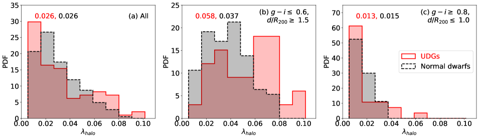
Figure 7: Distribution of halo spin parameters for all galaxies (left), blue field galaxies (middle), and red satellite galaxies (right). The UDGs are shown with red solid histograms, while normal dwarfs are shown with black dashed lines. The first and second numbers in the upper left corner of each panel give the medians for UDGs and normal dwarfs, respectively.

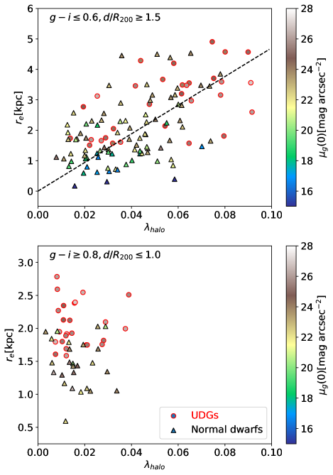
Figure 8: Relation between effective radius and halo spin for blue field galaxies (upper panel) and red satellites (lower panel). Circles and triangles denote UDGs and normal dwarfs, respectively. The color of each data point encodes the galaxy’s $g$-band central surface brightness, $\mu_{g}(0)$. The dashed line in the upper panel is a linear fit to all the data points.

The distributions of spin parameters for the whole UDG and normal dwarf samples are presented in the left panel of Fig. 7. The distributions are quite similar, and their median values are identical. A two-sample Kolmogorov-Smirnov (KS) test (two-sided) returns a KS statistic of $0.127$ and a p-value of $0.269$. However, if we split the sample into blue field galaxies (with $g-i\leq 0.6$ and $d/R_{200}\geq 1.5$) and red satellite galaxies (with $g-i\geq 0.8$ and $d/R_{200}\leq 1$), we can clearly see a significant difference between blue UDGs and normal dwarfs in the field, as shown in the middle panel. Note that we apply the additional colour restriction here in order to exclude backsplash field galaxies (whose properties are similar to satellite galaxies) and newly accreted satellites (whose properties are similar to field galaxies) so as not to contaminate either sample.

For blue field galaxies, UDGs tend to have higher halo spins than normal dwarfs. Their median spin ($0.058$) is $\sim 40$ per cent higher than that of normal dwarfs ($0.037$). The KS statistic is $0.393$ and the p-value is $1.10\times 10^{-3}$, indicating strong evidences to reject the null hypothesis that the halo spin parameters of these UDGs and normal dwarfs have the same distribution. If the blue field UDGs originate from high-spin haloes, we should expect to see a correlation between their sizes and spins, as suggested by semi-analytical models (e.g. Mo, Mao & White, 1998). In the upper panel of Fig. 8, we plot the relation between $r_{e}$ and $\lambda_{\mathrm{halo}}$ for blue field galaxies. We do see a clear correlation between galaxies’ effective radii and spin parameters. Galaxies with higher spins tend to have more extended sizes. Similar correlations have also been observed for Auriga host galaxies (see Grand et al., 2017). In Fig. 8, the colours of the points encode the galaxies’ $g$-band central surface brightness. As we can see, those normal dwarfs which have relatively high spins and large sizes are actually quite close to the definition of UDGs (i.e. their $\mu_{g}(0)$ are close to $24$ mag arcsec^-2). Therefore, our results indicate that the simulated field UDGs support the high-spin explanation inferred from semi-analytical models (Amorisco & Loeb, 2016; Rong et al., 2017) and further supported by some recent observations (Leisman et al., 2017; Spekkens & Karunakaran, 2018).

In contrast, we do not see significant differences between the distributions of spin for red satellite UDGs and normal dwarfs (right panel of Fig. 7). Their median spins are almost indistinguishable (i.e. $0.013$ for UDGs and $0.015$ for normal dwarfs). The corresponding KS statistic is $0.192$ and the p-value is $0.674$. Comparing to field galaxies, these satellite galaxies tend to have lower spins. A similar phenomenon is also found in pure $N$-body simulations (Onions et al., 2013), and is possibly due to the effect of tidal stripping in removing the outer layers of subhaloes (Wang et al., 2015b). The low spins of red satellite UDGs here are also consistent with the recent observations of van Dokkum et al. (2019b), which show that the rotation of the Coma UDG, DF 44, is fairly small, with a maximum rotation velocity - dispersion ratio, $V_{\rm max}/\left<\sigma\right><0.12$ ($90\%$ confidence). In the lower panel of Fig. 8, we plot the relation between $r_{e}$ and $\lambda_{\mathrm{halo}}$ for red satellites. In general, we do not see any clear correlation between spin and size for red satellite galaxies.

One possible explanation for the lack of correlation seen in red satellites is that as these galaxies are accreted into their hosts, the tidal effects gradually erase the original correlation between spin and size. Another possibility is that some red satellite UDGs may not originate from high-spin haloes. We will investigate these possibilities in detail in later subsections.

Another evidence hinting that the field and satellite UDGs may have different formation mechanisms is the axial ratios of their stellar distributions. Here, the axial ratios are computed from the three eigenvalues of the inertia tensor defined in Eq. (1), $a\leq b\leq c$. In Fig. 9, we show the axial ratios $a/b$ and $b/c$ of blue field galaxies and red satellite galaxies with scatter plots. We also compute the triaxiality parameter (Franx et al., 1991),

$$T=\frac{c^{2}-b^{2}}{c^{2}-a^{2}},$$ (7)

to quantify whether a galaxy is prolate ($T=1$) or oblate ($T=0$), and the minor-to-major axial ratio, $a/c$, to quantify the sphericity of a galaxy. As we can see from the upper panel, the blue field UDGs tend to be oblate (or disk-like) as their $b/c$ tend to be $1$, their median triaxiality is $0.26$ and their median $a/c$ is only $0.34$. This suggests that these blue field UDGs are disk galaxies similar to the classical low surface brightness galaxies. In contrast, the red satellite UDGs shown in the lower panel tend to be spherical as both their $a/b$ and $b/c$ are very close to $1$, and their median $a/c$ is $0.82$. This is consistent with the observational results that UDGs in clusters are usually round (van Dokkum et al., 2015; Koda et al., 2015; Yagi et al., 2016). The red satellite UDGs have a median triaxiality of $0.55$, which indicates that they are slightly more close to be prolate, in agreement with the results of Burkert (2017). This hints that the red satellite UDGs may have a different formation mechanism (e.g. tidal effects) from the blue field ones, which we will discuss in later subsections. Note that similar environmental dependencies of UDG morphology have been also found in Mancera Piña et al. (2019) for eight nearby clusters.

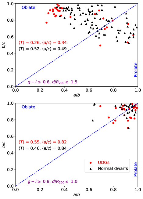
Figure 9: Axial ratios of stellar distribution within $2r_{\star,1/2}$ for blue field galaxies (upper panel) and red satellite galaxies (lower panel). UDGs and normal dwarfs are plotted with red circles and black triangles respectively. The dashed line indicates $b/c=a/b$. $\left<T\right>$ and $\left<a/c\right>$ with red (black) color give the median triaxiality and minor-to-major axial ratio for UDGs (normal dwarfs) respectively.

4.2 Density profile evolution of field UDGs

In this subsection we look at the evolution of the density profiles of field UDGs and normal dwarfs, and compare them with the results of Di Cintio et al. (2017) in order to investigate feedback outflows as the origin of UDGs.

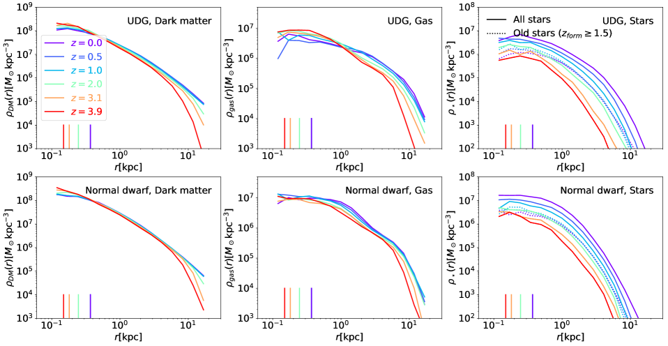
Figure 10: Evolution of stacked density profiles from $10$ selected UDGs (upper panel) and $10$ selected normal dwarfs (lower panel) in the field. All stacked UDGs and normal dwarfs have stellar masses in the range $[5\times 10^{7},5\times 10^{8}]{\rm M}_{\odot}$. From left to right, we plot the spherically-averaged density profiles for dark matter, gas, and star components respectively. The colors denoting different redshifts are specified in the legend in the upper left panel. In the right panels, we use solid lines and dotted lines to represent the density profiles of all stars and old stars (i.e. stars form before $z=1.5$), respectively. The vertical line segments in each panel mark the physical softening length at different redshifts. Note that after $z=1$, the physical softening length is fixed to $0.369$ kpc.

We compare the evolution of spherically-averaged dark matter, gas, and stellar density profiles for field UDGs and normal dwarfs in Fig. 10. To reduce noise, we have stacked $10$ UDGs and $10$ normal dwarfs with stellar masses in the range of $[5\times 10^{7},5\times 10^{8}]{\rm M}_{\odot}$. To emphasize the difference, we require the selected UDGs to have relatively larger sizes (i.e. $r_{e}\geq 2.5$ kpc), and the selected normal dwarfs to have smaller sizes (i.e. $r_{e}\leq 1.5$ kpc). We also require that the selected galaxies should never have been satellite galaxies. The mean stellar mass, effective radius, central $g$-band surface brightness, Sérsic index, and halo spin for the selected UDGs are $1.36\times 10^{8}{\rm M}_{\odot}$, $3.55$ kpc, $25.1$ mag arcsec^-2, $0.61$ and $0.061$, respectively, while for the selected normal dwarfs, they are $1.47\times 10^{8}{\rm M}_{\odot}$, $1.04$ kpc, $19.0$ mag arcsec^-2, $2.19$, and $0.032$, respectively.

The evolution of dark matter density profiles from $z=4$ to $0$ is presented in the left column of Fig. 10. A common feature of the Auriga dwarf galaxies is that their dark matter density profiles do not form cores and remain cuspy at all times (see a detailed study in Bose et al., 2019). This is different from the case of Di Cintio et al. (2017), where they suggest that the core creation mechanism is associated with the extended sizes of UDGs. As shown by Benítez-Llambay et al. (2019), this core-cusp difference is likely due to the different gas density thresholds for star formation adopted in different simulations (e.g. $n_{\mathrm{th}}=0.13$ cm^-3 for the Auriga simulations and $n_{\mathrm{th}}=10.3$ cm^-3 for NIHAO simulations); see also Dutton et al. (2019). Comparing the upper and lower panels in the left column of Fig. 10, it is notable that the density profiles of UDGs tend to evolve slighly more after $z=4$ than those of normal dwarfs.

The middle column of Fig. 10 shows the evolution of the gas density profiles. Comparing to the gas distribution at $z=4$, normal dwarfs tend to have more gas growth at small radii (i.e. $r\la 2$ kpc), while UDGs tend to have more gas growth at large radii (i.e. $r\ga 3$ kpc). This can be understood as a sign that gas in UDGs generally has higher specific angular momentum and thus a more extended distribution. Once the gas cools and forms stars, we can expect to see a similarly extended distribution of stars. As discussed in the following, this is indeed seen in the stellar density profiles.

In the right column of Fig. 10, we present the evolution of the stellar density profiles for UDGs and normal dwarfs. From $z=4$ to $0$, the stellar density profiles for both UDGs and normal dwarfs keep growing at all radii. However, compared to the stellar distribution at $z=4$, UDGs tend to have more star formation at large radii (i.e. $r\ga 2$ kpc), which is a result of high spin causing UDGs to be more extended. In this panel, we also plot the density profiles of old stars, defined as those formed before $z=1.5$, with dotted lines. The distribution of old stars evolves slightly with redshift. These results are different from those in Di Cintio et al. (2017), in which the central stellar density decreases by approximately one order of magnitude from $z=4$ to $0$ and the old stars expand dramatically in response to the supernovae feedback processes. Therefore, in the Auriga simulations we do not find the evolutionary picture expected from the feedback outflow scenario for field UDGs. Instead, our simulations support the high-spin origin of these galaxies.

4.3 Formation paths of satellite UDGs

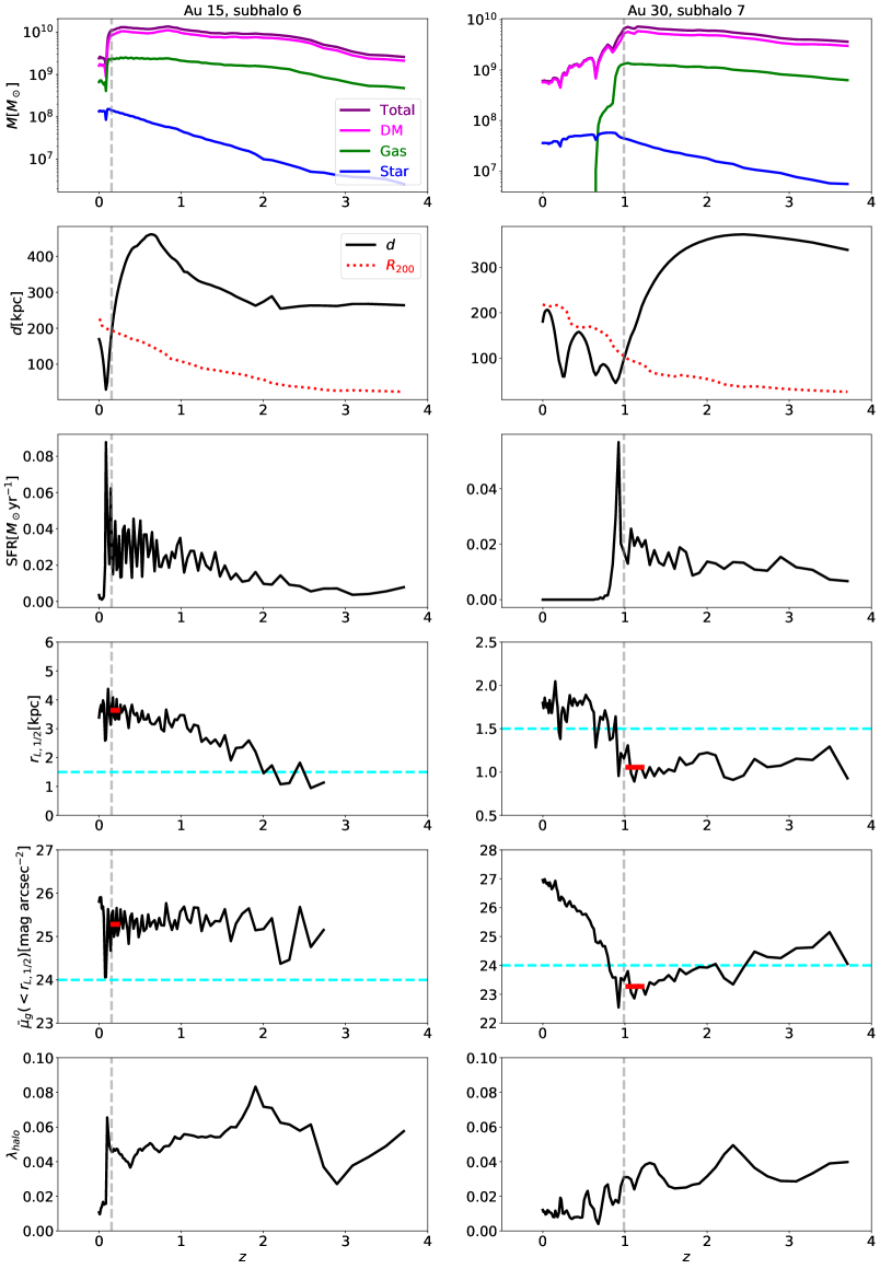
Figure 11: Evolutionary histories of two satellite UDGs, Au-15, Subhalo 6 (left) and Au-30, Subhalo 7 (right). From top to bottom, we plot the masses of the subhalo’s different components, distance from the subhalo to the host galaxy $d$ and the host galaxy’s $R_{200}$, star formation rate, half-light radius, $r_{L,1/2}$, mean surface brightness within $r_{L,1/2}$, and subhalo spin as a function of redshift. The grey dashed vertical lines mark the infall redshifts. The cyan horizontal dashed lines mark the thresholds used to define UDGs, i.e. $r_{L,1/2}=1.5$ kpc and $\bar{\mu}_{g}(<r_{L,1/2})=24$ mag arcsec^-2. In the fourth and fifth rows, the red line segments mark the mean values of $r_{L,1/2}$ and $\bar{\mu}_{g}(<r_{L,1/2})$ for five snapshots before infall, respectively.

Given that there is no evident correlation between $r_{e}$ and $\lambda_{\mathrm{halo}}$ for red satellite UDGs, a natural question is how such red satellite UDGs form. To answer this, we have traced the histories of satellite UDGs by following merger trees in our simulations. We find two distinct evolutionary paths: (i) a field origin in which the galaxy is a UDG before accretion and remains so up to the present day; (ii) a tidal origin in which the galaxy is a normal field dwarf before accretion but turns into a UDG after infall.

We first use two representative UDGs to illustrate these two formation paths. In Fig. 11, from top to bottom, we plot the time evolution of the masses of the different galaxy components, distance from the UDG to its host galaxy, $d$, and $R_{200}$ of the host, star formation rate (SFR), projected half-light radius, $r_{L,1/2}$, projected mean surface brightness within $r_{L,1/2}$, and the spin parameter of the dark matter subhalo. The fitted $r_{e}$ and $\mu_{g}(0)$ for UDGs at different redshifts are relatively noisy, especially at the redshifts when the UDGs experience significant tidal effects. Therefore, we use the half-light radius and mean surface brightness instead in the fourth and fifth rows of the figure. After projecting the star particles into the face-on plane, $r_{L,1/2}$ is defined as the radius where the enclosed luminosity is half of the total luminosity in the $g$-band, and $\bar{\mu}_{g}(<r_{L,1/2})$ is computed as the total $g$-band luminosity within $r_{L,1/2}$ divided by the area, $\pi r_{L,1/2}^{2}$. We adopt similar criteria to define a UDG at high redshift: $r_{L,1/2}\geq 1.5$ kpc and $\bar{\mu}_{g}(<r_{L,1/2})\geq 24$ mag arcsec^-2, which are plotted as cyan dashed horizontal lines in the fourth and fifth rows.

Let us first look at the satellite UDG (Au-15, Subhalo 6) shown in the left column of Fig. 11, which is an example of “field origin”. The progenitor of this UDG falls into the host galaxy recently at $z_{\mathrm{infall}}=0.17$ (marked by the grey dashed vertical line). The infall redshift is here defined as the redshift when the progenitor first enters the virial radius of its host galaxy. Before infall, the progenitor resides in a dark matter halo with a relatively high spin parameter, around $0.06$. As illustrated in the previous sections, this high spin has kept the galaxy size increasing all the time. At $z\sim 2$, the progenitor becomes a UDG. After $z=2$, the progenitor still contains enough gas to power star formation at a rate of $\sim 0.02{\rm M}_{\odot}\mathrm{yr}^{-1}$. The mean surface brightness within the half-light radius is roughly constant for this galaxy before $z_{\mathrm{infall}}$. Prior to its infall, the progenitor has a size of $r_{L,1/2}=3.64$ kpc and a mean surface brightness $\bar{\mu}_{g}(<r_{L,1/2})=25.28$ mag arcsec^-2. After infall, a significant amount of dark matter and gas are tidally stripped during the first pericentric passage, and star formation is almost halted. The stellar component is also affected by the tidal process, leading to larger fluctuations in $r_{L,1/2}$ and $\bar{\mu}_{g}(<r_{L,1/2})$. The UDG recovers after passing pericenter, and remains as a UDG. We also observe that tidal stripping has greatly reduced the spin of the associated dark matter halo, which is consistent with previous studies (e.g. Onions et al., 2013; Wang et al., 2015b). The idea that some satellite UDGs originate from infalling field UDGs is consistent with some observational results (Román & Trujillo, 2017a, b; Alabi et al., 2018).

The satellite UDG (Au-30, Subhalo 7) shown in the right column of Fig. 11 illustrates an example of a UDG forming through the “tidal origin” channel. It has an earlier infall time, $z_{\mathrm{infall}}=1.04$. Before $z_{\mathrm{infall}}$, the progenitor is a normal dwarf in the field and resides in a dark matter halo with a relatively low spin (i.e. $\sim 0.035$). It is gas rich, and has an SFR around $0.015{\rm M}_{\odot}\mathrm{yr}^{-1}$. The galaxy size is almost constant ($r_{L,1/2}\sim 1$ kpc), while the mean central surface brightness keeps increasing ($\bar{\mu}_{g}(<r_{L,1/2})$ drops from $\sim 25$ to $\sim 23$ mag arcsec^-2). This indicates that the newly formed stars are mainly created in the central region. After the progenitor falls into the host galaxy, its dark matter and gas components are severely stripped, specially the gas which is fully stripped by ram pressure during the second orbit, and the galaxy is quenched (e.g. its SFR becomes zero thereafter). At the same time, the galaxy size keeps growing during each orbital passage, whilst the central surface brightness keeps decreasing mainly because of passive evolution. The progenitor becomes a UDG after the second pericentric passage. Clearly, it is the tidal effect that transforms this normal dwarf into a UDG. The tidal origin mechanism seen in our simulations is supported by observations of some UDGs which are associated with tidal features (see e.g. Mihos et al., 2015; Crnojević et al., 2016; Merritt et al., 2016; Toloba et al., 2016; Venhola et al., 2017; Wittmann et al., 2017; Greco et al., 2018; Toloba et al., 2018). The claimed UDG in our Milky Way Galaxy, Sagittarius dSph, can also be regarded as an example of a UDG of tidal origin.

Following the illustration of two individual cases of two different origins for satellite UDGs, the next question is: what are the fractions of our simulated satellite UDGs that have these two different origins? To answer this question, we divided the satellite UDGs into two subsamples according to whether they are UDGs before accretion or not. When determining whether a progenitor is a UDG, in order to reduce noise, we used the mean values of $r_{L,1/2}$ and $\bar{\mu}_{g}(<r_{L,1/2})$ from five snapshots prior to the infall snapshot (as shown in the fourth and fifth rows of Fig. 11 with red line segments). At $z\leq 4$, the time interval between two successive snapshots is $0.1-0.2$ Gyr. We find that, for the $38$ satellite UDGs in our sample, $21$ $(55\%)$ of them have a field origin, while the remaining $17$ $(45\%)$ have a tidal origin. The satellite UDGs with a field origin tend to have a later infall time (i.e. with a median infall redshift of $0.55$) than those with a tidal origin (i.e. with a median infall redshift of $1.04$). The recent simulation work of Jiang et al. (2019), which studies satellite UDGs in a group environment, also finds similar formation paths and fractions.

An intriguing aspect of satellite UDGs in observations is that they tend to have higher specific frequency of globular clusters than normal dwarfs with similar luminosity. For example, UDGs in the Coma cluster are found to have on average $\sim 7$ times more globular clusters than other galaxies of the same luminosity (van Dokkum et al. 2017; see also Beasley et al. 2016; Peng & Lim 2016; Amorisco et al. 2018; Lim et al. 2018), albeit with large scatters (Amorisco et al., 2018); the confirmed globular clusters in NGC1052-DF2 and NGC1052-DF4 make up $\sim 3\%$ of the galaxy total luminosity (van Dokkum et al., 2018b; van Dokkum et al., 2019a), which is much higher than known normal dwarfs. As globular clusters are not resolved in our simulations, and high spins and tidal interactions do not directly enhance the number of globular clusters (Peng & Lim, 2016; Lim et al., 2018), it will be interesting to study why UDGs have higher abundance of globular clusters than normal dwarfs with the next generation hydrodynamical simulations.

5 Conclusions

In this paper we have investigated the formation of UDGs in the vicinity of Milky Way-sized galaxies in the Auriga cosmological magento-hydrodynamics simulations. We identified a total of $92$ UDGs in $30$ high-resolution Auriga simulations, which enables us to explore the properties and origin of UDGs with good statistics. We show that the Auriga simulations reproduce key observed properties of UDGs, including sizes, central surface brightness, absolute magnitudes, Sérsic indices, colors, spatial distribution and abundance. The Auriga UDGs have similar masses to normal dwarfs and can be seen as extreme versions of normal dwarfs rather than as a distinct population.

Field UDGs in the simulations reside in low-mass haloes and have larger spin parameters than normal dwarfs; their low surface brightness merely reflects a strong correlation between their effective radii and their halo spins. The evolution of the dark matter, gas and star density profiles in the field UDGs in the Auriga simulations is very different from that in the NIHAO and FIRE simulations where the UDGs result from strong supernova feedback (Di Cintio et al., 2017; Chan et al., 2018). The Auriga simulations support the high-spin origin of field UDGs inferred from semi-analytical models (Amorisco & Loeb, 2016; Rong et al., 2017).

Satellite UDGs in the Auriga simulations have two distinct origins: (i) field dwarfs that are UDGs before accretion and remain UDGs to the present day; (ii) galaxies that are normal dwarfs before accretion but are subsequently transformed into UDGs by strong tidal interactions. About $\sim 55\%$ of the $38$ satellite UDGs in our sample have a field origin, while the remaining $\sim 45\%$ have a tidal origin.

Appendix A Resolution study

The Auriga simulations include six runs (i.e. Au-6, Au-16, Au-21, Au-23, Au-24, and Au-27) with higher resolutions, i.e. $m_{\mathrm{DM}}=4\times 10^{4}{\rm M}_{\odot}$, $m_{\mathrm{b}}=6\times 10^{3}{\rm M}_{\odot}$, and $\epsilon=184$ pc at $z=0$. This set of higher-resolution simulations is named ‘Level-3 (L3)’ simulations, and the $30$ Auriga simulations with lower resolutions are called ‘Level-4 (L4)’ simulations. Currently, it is still difficult to perform one-to-one match and comparisons for galaxies in hydrodynamical simulations with different resolutions. Here, we address the resolution convergence of L4 simulations by looking at the statistical properties of UDGs identified from simulations with different resolutions.

Following the methods outlined in Section 2.2, we identify UDGs from six L3 simulations. The only difference is that we adopt $20$ logarithmic bins in $r$ when computing the projected $g$-band surface brightness profiles, and we have checked that our results are not sensitive to the number of radial bins. In total, there are $14$ UDGs ($8$ field UDGs $+$ $6$ satellite UDGs) identified from these six L3 simulations. As a comparison, in the corresponding six L4 simulations, we find $16$ UDGs ($10$ field UDGs $+$ $6$ satellite UDGs). The general properties of UDGs from L4 and L3 simulations are compared in Table 2.

Overall, UDGs from L4 and L3 simulations agree well in different properties. This indicates that Auriga simulations achieve relatively good resolution convergence in galaxy properties, consistent also with Marinacci, Pakmor & Springel (2014).

Table 2: Properties of UDGs identified from the L4 and L3 simulations. Apart from the number of UDGs, other rows show the mean values and standard deviations of different physical quantities.

	L4	L3
# of UDGs	$16$	$14$
# of field UDGs	$10$	$8$
# of satellite UDGs	$6$	$6$
$r_{e}$ [kpc]	$2.19\pm 0.83$	$2.20\pm 0.72$
$\mu_{g}(0)$ [mag arcsec-2]	$25.3\pm 0.43$	$25.2\pm 0.97$
Sérsic $n$	$0.95\pm 0.33$	$0.84\pm 0.33$
$g-i$	$0.76\pm 0.25$	$0.60\pm 0.28$
$M_{\star}$ [${\rm M}_{\odot}$]	$10^{7.7\pm 0.37}$	$10^{7.6\pm 0.48}$
$M_{\mathrm{halo}}$ [${\rm M}_{\odot}$]	$10^{9.4\pm 0.55}$	$10^{9.4\pm 0.61}$

References

- Alabi et al. (2018) Alabi A., et al., 2018, MNRAS, 479, 3308
- Amorisco & Loeb (2016) Amorisco N. C., Loeb A., 2016, MNRAS, 459, L51
- Amorisco et al. (2018) Amorisco N. C., Monachesi A., Agnello A., White S. D. M., 2018, MNRAS, 475, 4235
- Beasley & Trujillo (2016) Beasley M. A., Trujillo I., 2016, ApJ, 830, 23
- Beasley et al. (2016) Beasley M. A., Romanowsky A. J., Pota V., Navarro I. M., Martinez Delgado D., Neyer F., Deich A. L., 2016, ApJ, 819, L20
- Bellazzini et al. (2017) Bellazzini M., Belokurov V., Magrini L., Fraternali F., Testa V., Beccari G., Marchetti A., Carini R., 2017, MNRAS, 467, 3751
- Benítez-Llambay et al. (2019) Benítez-Llambay A., Frenk C. S., Ludlow A. D., Navarro J. F., 2019, MNRAS, 488, 2387
- Bose et al. (2019) Bose S., et al., 2019, MNRAS, 486, 4790
- Boylan-Kolchin et al. (2009) Boylan-Kolchin M., Springel V., White S. D. M., Jenkins A., Lemson G., 2009, MNRAS, 398, 1150
- Burkert (2017) Burkert A., 2017, ApJ, 838, 93
- Carleton et al. (2019) Carleton T., Errani R., Cooper M., Kaplinghat M., Peñarrubia J., Guo Y., 2019, MNRAS, 485, 382
- Chan et al. (2018) Chan T. K., Kereš D., Wetzel A., Hopkins P. F., Faucher-Giguère C.-A., El-Badry K., Garrison-Kimmel S., Boylan-Kolchin M., 2018, MNRAS, 478, 906
- Cohen et al. (2018) Cohen Y., et al., 2018, ApJ, 868, 96
- Crnojević et al. (2016) Crnojević D., et al., 2016, ApJ, 823, 19
- Dalcanton et al. (1997) Dalcanton J. J., Spergel D. N., Gunn J. E., Schmidt M., Schneider D. P., 1997, AJ, 114, 635
- Danieli & van Dokkum (2019) Danieli S., van Dokkum P., 2019, ApJ, 875, 155
- Davis et al. (1985) Davis M., Efstathiou G., Frenk C. S., White S. D. M., 1985, ApJ, 292, 371
- Di Cintio et al. (2017) Di Cintio A., Brook C. B., Dutton A. A., Macciò A. V., Obreja A., Dekel A., 2017, MNRAS, 466, L1
- Digby et al. (2019) Digby R., et al., 2019, MNRAS, 485, 5423
- Dutton et al. (2019) Dutton A. A., Macciò A. V., Buck T., Dixon K. L., Blank M., Obreja A., 2019, MNRAS, 486, 655
- Ferré-Mateu et al. (2018) Ferré-Mateu A., et al., 2018, MNRAS, 479, 4891
- Franx et al. (1991) Franx M., Illingworth G., de Zeeuw T., 1991, ApJ, 383, 112
- Gao et al. (2012) Gao L., Navarro J. F., Frenk C. S., Jenkins A., Springel V., White S. D. M., 2012, MNRAS, 425, 2169
- Garrison-Kimmel et al. (2019) Garrison-Kimmel S., et al., 2019, MNRAS, 487, 1380
- Grand et al. (2017) Grand R. J. J., et al., 2017, MNRAS, 467, 179
- Greco et al. (2018) Greco J. P., et al., 2018, PASJ, 70, S19
- Gu et al. (2018) Gu M., et al., 2018, ApJ, 859, 37
- Guo et al. (2011) Guo Q., et al., 2011, MNRAS, 413, 101
- Hopkins et al. (2018) Hopkins P. F., et al., 2018, MNRAS, 480, 800
- Ibata et al. (1994) Ibata R. A., Gilmore G., Irwin M. J., 1994, Nature, 370, 194
- Impey et al. (1988) Impey C., Bothun G., Malin D., 1988, ApJ, 330, 634
- Janssens et al. (2017) Janssens S., Abraham R., Brodie J., Forbes D., Romanowsky A. J., van Dokkum P., 2017, ApJ, 839, L17
- Jiang et al. (2019) Jiang F., Dekel A., Freundlich J., Romanowsky A. J., Dutton A. A., Macciò A. V., Di Cintio A., 2019, MNRAS, 487, 5272
- Kadowaki et al. (2017) Kadowaki J., Zaritsky D., Donnerstein R. L., 2017, ApJ, 838, L21
- Karachentsev et al. (2017) Karachentsev I. D., Makarova L. N., Sharina M. E., Karachentseva V. E., 2017, Astrophysical Bulletin, 72, 376
- Koda et al. (2015) Koda J., Yagi M., Yamanoi H., Komiyama Y., 2015, ApJ, 807, L2
- Kubo et al. (2007) Kubo J. M., Stebbins A., Annis J., Dell’Antonio I. P., Lin H., Khiabanian H., Frieman J. A., 2007, ApJ, 671, 1466
- Lee et al. (2017) Lee M. G., Kang J., Lee J. H., Jang I. S., 2017, ApJ, 844, 157
- Leisman et al. (2017) Leisman L., et al., 2017, ApJ, 842, 133
- Lim et al. (2018) Lim S., Peng E. W., Côté P., Sales L. V., den Brok M., Blakeslee J. P., Guhathakurta P., 2018, ApJ, 862, 82
- Makarov et al. (2015) Makarov D. I., Sharina M. E., Karachentseva V. E., Karachentsev I. D., 2015, A&A, 581, A82
- Mancera Piña et al. (2018) Mancera Piña P. E., Peletier R. F., Aguerri J. A. L., Venhola A., Trager S., Choque Challapa N., 2018, MNRAS, 481, 4381
- Mancera Piña et al. (2019) Mancera Piña P. E., Aguerri J. A. L., Peletier R. F., Venhola A., Trager S., Choque Challapa N., 2019, MNRAS, 485, 1036
- Marinacci et al. (2014) Marinacci F., Pakmor R., Springel V., 2014, MNRAS, 437, 1750
- Martínez-Delgado et al. (2016) Martínez-Delgado D., et al., 2016, AJ, 151, 96
- Merritt et al. (2016) Merritt A., van Dokkum P., Danieli S., Abraham R., Zhang J., Karachentsev I. D., Makarova L. N., 2016, ApJ, 833, 168
- Mihos et al. (2015) Mihos J. C., et al., 2015, ApJ, 809, L21
- Mihos et al. (2017) Mihos J. C., Harding P., Feldmeier J. J., Rudick C., Janowiecki S., Morrison H., Slater C., Watkins A., 2017, ApJ, 834, 16
- Mo et al. (1998) Mo H. J., Mao S., White S. D. M., 1998, MNRAS, 295, 319
- Mowla et al. (2017) Mowla L., van Dokkum P., Merritt A., Abraham R., Yagi M., Koda J., 2017, ApJ, 851, 27
- Muñoz et al. (2015) Muñoz R. P., et al., 2015, ApJ, 813, L15
- Müller et al. (2018) Müller O., Jerjen H., Binggeli B., 2018, A&A, 615, A105
- Navarro et al. (2010) Navarro J. F., et al., 2010, MNRAS, 402, 21
- Onions et al. (2013) Onions J., et al., 2013, MNRAS, 429, 2739
- Pandya et al. (2018) Pandya V., et al., 2018, ApJ, 858, 29
- Papastergis et al. (2017) Papastergis E., Adams E. A. K., Romanowsky A. J., 2017, A&A, 601, L10
- Peng & Lim (2016) Peng E. W., Lim S., 2016, ApJ, 822, L31
- Planck Collaboration et al. (2014) Planck Collaboration et al., 2014, A&A, 571, A16
- Román & Trujillo (2017a) Román J., Trujillo I., 2017a, MNRAS, 468, 703
- Román & Trujillo (2017b) Román J., Trujillo I., 2017b, MNRAS, 468, 4039
- Rong et al. (2017) Rong Y., Guo Q., Gao L., Liao S., Xie L., Puzia T. H., Sun S., Pan J., 2017, MNRAS, 470, 4231
- Ruiz-Lara et al. (2018) Ruiz-Lara T., et al., 2018, MNRAS, 478, 2034
- Schaye et al. (2015) Schaye J., et al., 2015, MNRAS, 446, 521
- Shi et al. (2017) Shi D. D., et al., 2017, ApJ, 846, 26
- Sifón et al. (2018) Sifón C., van der Burg R. F. J., Hoekstra H., Muzzin A., Herbonnet R., 2018, MNRAS, 473, 3747
- Simpson et al. (2018) Simpson C. M., Grand R. J. J., Gómez F. A., Marinacci F., Pakmor R., Springel V., Campbell D. J. R., Frenk C. S., 2018, MNRAS, 478, 548
- Smith Castelli et al. (2016) Smith Castelli A. V., Faifer F. R., Escudero C. G., 2016, A&A, 596, A23
- Spekkens & Karunakaran (2018) Spekkens K., Karunakaran A., 2018, ApJ, 855, 28
- Springel (2010) Springel V., 2010, MNRAS, 401, 791
- Springel et al. (2001) Springel V., White S. D. M., Tormen G., Kauffmann G., 2001, MNRAS, 328, 726
- Springel et al. (2005) Springel V., et al., 2005, Nature, 435, 629
- Toloba et al. (2016) Toloba E., et al., 2016, ApJ, 816, L5
- Toloba et al. (2018) Toloba E., et al., 2018, ApJ, 856, L31
- Trujillo et al. (2017) Trujillo I., Roman J., Filho M., Sánchez Almeida J., 2017, ApJ, 836, 191
- Venhola et al. (2017) Venhola A., et al., 2017, A&A, 608, A142
- Wang et al. (2015a) Wang L., Dutton A. A., Stinson G. S., Macciò A. V., Penzo C., Kang X., Keller B. W., Wadsley J., 2015a, MNRAS, 454, 83
- Wang et al. (2015b) Wang Y., Lin W., Pearce F. R., Lux H., Muldrew S. I., Onions J., 2015b, ApJ, 801, 93
- Wittmann et al. (2017) Wittmann C., et al., 2017, MNRAS, 470, 1512
- Yagi et al. (2016) Yagi M., Koda J., Komiyama Y., Yamanoi H., 2016, ApJS, 225, 11
- Yozin & Bekki (2015) Yozin C., Bekki K., 2015, MNRAS, 452, 937
- Zaritsky (2017) Zaritsky D., 2017, MNRAS, 464, L110
- van Dokkum et al. (2015) van Dokkum P. G., Abraham R., Merritt A., Zhang J., Geha M., Conroy C., 2015, ApJ, 798, L45
- van Dokkum et al. (2016) van Dokkum P., et al., 2016, ApJ, 828, L6
- van Dokkum et al. (2017) van Dokkum P., et al., 2017, ApJ, 844, L11
- van Dokkum et al. (2018a) van Dokkum P., et al., 2018a, Nature, 555, 629
- van Dokkum et al. (2018b) van Dokkum P., et al., 2018b, ApJ, 856, L30
- van Dokkum et al. (2019a) van Dokkum P., Danieli S., Abraham R., Conroy C., Romanowsky A. J., 2019a, ApJ, 874, L5
- van Dokkum et al. (2019b) van Dokkum P., et al., 2019b, ApJ, 880, 91
- van der Burg et al. (2016) van der Burg R. F. J., Muzzin A., Hoekstra H., 2016, A&A, 590, A20
- van der Burg et al. (2017) van der Burg R. F. J., et al., 2017, A&A, 607, A79