Minimal Length Effects on Quantum Cosmology and Quantum Black Hole Models

Abstract

A Kantowski-Sachs model with a modified quantization prescription is considered. Such quantization rules, inspired by the so-called Generalized Uncertainty Principle (GUP), correspond to a modified commutation relation between minisuperspace variables and their conjugate momenta. For a wide range of the modification parameter, this approach differentiates from the standard results by the presence of a potential well in the corresponding Wheeler-DeWitt equation. This then produces the appearance of a set of wave functions, with corresponding discrete energy spectrum.

I Introduction

Among the most tenacious efforts in fundamental physics is the seek for a theory of Quantum Gravity (QG), that is, a theory that could give a quantum description of gravity. As of now, several candidates have been proposed, and the debate on the validity of one over the others is open. Despite the various theoretical possibilities to realize a theory of QG, no experimental evidence can direct us, nor any evidence of deviations from general relativity or quantum theories can help us in this task. Nonetheless, there are a series of features that we expect from a quantum theory of gravity. On of these features, when translated to low energy systems, consists in the existence of a minimal measurable length Garay1995_1 . In fact, such a minimal length arises in different contexts, for example from string theory Gross1988_1 ; Amati1989_1 , loop quantum gravity Rovelli1995 ; Rovelli1998 ; Ashtekar2017 , and thought experiments in black hole physics Maggiore1993_1 ; Scardigli1999_1 . These common characteristics of several theories of quantum gravity led to a phenomenological model consisting in a modification of the uncertainty principle. Such a model is known as the generalized uncertainty principle (GUP). It has been the subject of many studies, in the attempt to use it as a signature of QG, and has been compared with known phenomena and theories of modified gravity (see, e.g., Scardigli2016 ; Scardigli2016_1 ; Bosso2017 ; Lambiase2018 ; Bosso2018_1 ; Scardigli2018 ; Kanazawa2019 ; Buoninfante2019 ; Bushev2019 ). A version of this model considers a modification of the Heisenberg algebra Kempf1995_1 ; Das2009_1 ; BossoPhD ; Bosso2018 to reproduce, via the Schrödinger–Robertson uncertainty relation, the desired minimal length. Notice that this modification can also be thought of as a modified quantization rule.

These effects are predicted to be important in systems with energies near the Planck scale. A particularly relevant example of such systems is the very early universe, in which quantum effects of gravity are expected to be dominant Ryan1972 ; Hartle1983 ; Ryan2015 . A special branch of this line of investigation is loop quantum cosmology, developed in the past years, where the framework of loop quantum gravity has been applied to cosmology Ashtekar2011 ; Agullo2017 . Therefore, Quantum Cosmology is the appropriate playground where this modified quantization rule is expected to be influential. Previous approaches to this field using the tools of canonical quantum gravity have investigated various aspects of this construction with the purpose of studying quantum cosmological models. In the past, several quantization procedures have been considered regarding this approximation (see, e.g. Bergeron2017 ). In particular, recent attempts have been directed towards a noncommutative deformation of quantum cosmology Garcia-Compean2002 ; Aguero2007 , that is, descriptions in which variables do not commute. This resulted from proposals of noncommutativity in spacetime and from developments in $M$ theory and string theory Snyder1947 ; Connes1995 ; Douglas2001 .

In the present work, thus, we implement a different perspective, proposing a quantization rule for the minisuperspace approximation Misner1969 ; Misner1972 in which the corresponding variables are considered to obey a similar commutation relation as in GUP. This will imply a modification of the Wheeler-DeWitt equation (WDWE), governing the quantum cosmological model, characterizing a modified dynamics of the solution. Previous approaches from a different viewpoint have been pursued in Kober2011 ; Faizal2014 ; Garattini2016 . It is worth noticing that this procedure does not directly implies a physical minimal length. Rather, it can be understood as imposing a minimal uncertainty in the minisuperspace variables.

As a particular case for this proposal, we will consider its effects on the Kantowski-Sachs model. As it is known, at the classical level it describes a homogeneous but anisotropic cosmological model, thus not relatable with the current description with the observable universe Obregon1998 . However, its relevance arises as well from the fact that it can describe a Schwarzschild black hole Gambini2015 . The wave function of the corresponding quantum model thus represents a quantum cosmology or a quantum black hole. The minisuperspace coordinates, at the present quantum stage, are not affected by their classical dependence on the time $t$ or the radius $r$ Obregon1998 . Thus, from now on, we will refer our analysis only at the level of the minisuperspace Kantowski-Sachs variables and their quantum evolution. This metric can be written as Misner1972

$$\mathrm{d}s^{2}=-N^{2}\mathrm{d}t^{2}+e^{2\sqrt{3}\beta}\mathrm{d}r^{2}\\ +e^{-2\sqrt{3}\beta}e^{-2\sqrt{3}\Omega}(\mathrm{d}\theta^{2}+\sin^{2}\theta\mathrm{d}\phi^{2}).$$ (1)

The corresponding WDWE in the standard theory of quantum gravity is given by

$$e^{\sqrt{3}\beta+2\sqrt{3}\Omega}\left[-P_{\Omega}^{2}+P_{\beta}^{2}-48e^{-2\sqrt{3}\Omega}\right]\psi(\Omega,\beta)=0,$$ (2)

where

$$P_{\Omega}= -i\frac{\partial}{\partial\Omega}, P_{\beta}= -i\frac{\partial}{\partial\beta},$$ (3)

are the conjugate momenta to the variables $\Omega$ and $\beta$, respectively, and such that

$$[\Omega,P_{\Omega}]= i, [\beta,P_{\Omega}]= 0, [\Omega,P_{\beta}]= 0, [\beta,P_{\beta}]= i.$$ (4)

The solutions of Eq. (2) are given in terms of the modified Bessel function $K_{i\nu}$ as follows

$$\psi^{\pm}_{\nu}(\Omega,\beta)=e^{\pm i\nu\sqrt{3}\beta}K_{i\nu}(4e^{-\sqrt{4}\Omega}).$$ (5)

In what follows, we will revise the model above modifying the quantization relations in Eq. (4). In particular, we will consider a different commutation relation between the variables $\{\Omega,\beta\}$ and the conjugate momenta. In fact, we will consider the model inspired by Kempf1995_1 , for which

$$[q_{j},p_{k}]=i\delta_{jk}\{1+\gamma^{2}p_{l}p_{l}\},$$ (6)

with

$$q_{1}= \Omega, q_{2}= \beta, p_{1}= P_{\Omega}, p_{2}= P_{\beta},$$ (7)

where $\gamma$ is some parameter with units of inverse $P_{\Omega}$ and $P_{\beta}$, and where we considered Einstein’s summation convention. For a more convenient treatment, we will introduce coordinates $q^{\prime}_{j}$ such that $[q^{\prime}_{j},p_{k}]=i\delta_{jk}$, i.e. $q^{\prime}_{j}$ and $p_{k}$ fulfill the same relations as those in Eqs. (4). The momentum-space representation of the coordinate operators obeying Eqs. (6) is

$$q_{j}=i(1+\gamma^{2}p_{k}p_{k})\frac{\partial}{\partial p_{j}}=(1+\gamma^{2}p_{k}p_{k})q^{\prime}_{j}.$$ (8)

Notice that in this model, the two coordinates do not commute

$$[q_{j},q_{k}]=2i\gamma^{2}(1+\gamma^{2}p_{l}p_{l})(p_{j}q^{\prime}_{k}-p_{k}q^{\prime}_{j})=2\gamma^{2}\epsilon_{jk}p_{j}q_{k},$$ (9)

where $\epsilon_{jk}$ is the two-indices Levi-Civita symbol. Furthermore, in position-space we can write

$$q_{j}=q_{j}^{\prime}(1+\gamma^{2}p_{k}p_{k}).$$ (10)

As we will see next, this modification is directly related with the form of the wave function $\psi(\Omega,\beta)$ in Eq. (2) introducing, for a particular range of values for the parameter $\gamma$, a well in the potential in Eq. (2). The effect of this modification is to modify the uncertainty relation for the minisuperspace variables. In fact, it imposes a minimal uncertainty in these variables, thus resulting in a fuzy metric. As a consequence, this furthermore results in a notion of distance with a minimal uncertainty and, therefore, a minimal length.

This paper is structured as follows: in Section II, we will revise the WDWE for the Kantowski-Sachs model with a modified quantization rule; in Section III, we will focus on a particular region of the variables, in which the modified potential associated with the Kantowski-Sachs model produces a more noticeable difference with the usual quantum behavior Eq. (5); finally, Section IV is devoted to conclusions and outlook.

II Kantowski-Sachs model with GUP

Following Garcia-Compean2002 and using the relations above, the potential term in Eq. (2) can be rewritten as

$$V=-48e^{-2\sqrt{3}\Omega}=-48e^{-2\sqrt{3}\Omega^{\prime}[1+\gamma^{2}(-P_{\Omega}^{2}+P_{\beta}^{2})]}\\ \simeq-48e^{-2\sqrt{3}(1-4\gamma^{2})\Omega^{\prime}}e^{-2\sqrt{3}\gamma^{2}\Omega^{\prime}(-P_{\Omega}^{2}+P_{\beta}^{2})}e^{12i\gamma^{2}\Omega^{\prime}P_{\Omega}},$$ (11)

where Zassenhaus formula

$$e^{A+B}=e^{A}e^{B}e^{-\frac{1}{2}[A,B]}e^{\frac{1}{6}([A,[A,B]]+2[B,[A,B]])}\cdots\,,$$ (12)

has been used and where only terms up to exponentials in $\gamma^{2}$ have been retained. Using the substitution $\Omega^{\prime}=e^{x}$ we find

$$-i\Omega^{\prime}\frac{\partial}{\partial\Omega^{\prime}}=-i\frac{\partial}{\partial x}\,.$$ (13)

Therefore, assuming the following representation for the momentum operators

$$P_{\Omega}= -i\frac{\partial}{\partial\Omega^{\prime}}\,, P_{\beta}= -i\frac{\partial}{\partial\beta^{\prime}}\,,$$ (14)

the last exponential above, Eq. (11), acts as a translation operator for the coordinate $x$, corresponding to a scaling of the coordinate $\Omega^{\prime}$

$$e^{12i\gamma^{2}\Omega^{\prime}P_{\Omega}}\psi(\Omega^{\prime},\beta)=\psi(e^{12\gamma^{2}}\Omega^{\prime},\beta).$$ (15)

The potential above then becomes

$$V\psi(\Omega^{\prime},\beta^{\prime})=-48e^{-2\sqrt{3}(1-4\gamma^{2})\Omega^{\prime}}\\ \times e^{-2\sqrt{3}\gamma^{2}\Omega^{\prime}(-P_{\Omega}^{2}+P_{\beta}^{2})}\psi(e^{12\gamma^{2}}\Omega^{\prime},\beta^{\prime}).$$ (16)

We can further expand the second exponential in the previous expression up to second order in momentum, obtaining

$$V\simeq-48e^{-2\sqrt{3}(1-4\gamma^{2})\Omega^{\prime}}\left[1-2\sqrt{3}\gamma^{2}\Omega^{\prime}(-P_{\Omega}^{2}+P_{\beta}^{2})\right].$$ (17)

We can then rewrite the modified Eq. (2) as

$$\left[\left(1+96\sqrt{3}\gamma^{2}\Omega^{\prime}e^{-2\sqrt{3}(1-4\gamma^{2})\Omega^{\prime}}\right)\left(-P_{\Omega}^{2}+P_{\beta}^{2}\right)\right.\\ \left.-48e^{-2\sqrt{3}(1-4\gamma^{2})\Omega^{\prime}}\right]\psi(e^{12\gamma^{2}}\Omega^{\prime},\beta^{\prime})=0.$$ (18)

It is interesting to notice that the region in which the modification terms are relevant depends on $\gamma$. In fact, the closer $\gamma$ is to the value $1/2$, the more extended this region is and the more relevant the correction terms are, as shown in Fig. 1. We will focus on the interval of $\Omega^{\prime}$ in which the modification is not negligible, since outside this region the same results as in Misner1972 apply.

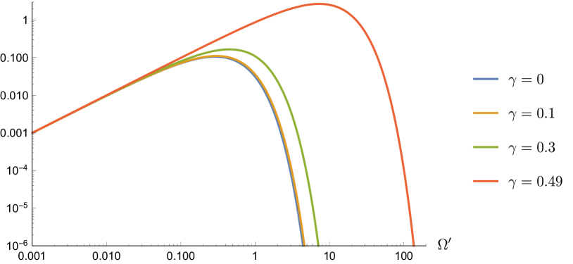
Figure 1: Functions $\Omega^{\prime}e^{-2\sqrt{3}(1-4\gamma^{2})\Omega^{\prime}}$. Notice that the interval of values of $\Omega^{\prime}$ in which the corrections are not negligible depends on the value of $\gamma$. In particular, the closer $\gamma$ is to the value $1/2$, the more extended and large in magnitude the modification is. The pick of this function is for $\Omega^{\prime}=\frac{1}{2\sqrt{3}(1-4\gamma^{2})}$.

Using the same factorization as in Garcia-Compean2002 ,

$$\psi(e^{12\gamma^{2}}\Omega^{\prime},\beta^{\prime})=e^{\sqrt{3}\nu\beta^{\prime}}\chi(\Omega^{\prime}),$$ (19)

we can write the previous equation up to second order in $\gamma$ as

$$\left[\frac{\mathrm{d}^{2}}{\mathrm{d}\Omega^{\prime}{}^{2}}-3\nu^{2}-\left(1-96\sqrt{3}\gamma^{2}\Omega^{\prime}e^{-2\sqrt{3}(1-4\gamma^{2})\Omega^{\prime}}\right)\right.\\ \left.\times 48e^{-2\sqrt{3}(1-4\gamma^{2})\Omega^{\prime}}\right]\chi(\Omega^{\prime})\\ =\left[-\frac{\mathrm{d}^{2}}{\mathrm{d}\Omega^{\prime}{}^{2}}-V_{\gamma,\nu}-\gamma^{2}\tilde{V}\right]\chi(\Omega^{\prime})=0,$$ (20)

where

$$V_{\gamma,\nu}= 3\nu^{2}+48e^{-2\sqrt{3}(1-4\gamma^{2})\Omega^{\prime}},$$ (21a)

$$\tilde{V}= -4608\sqrt{3}\Omega^{\prime}e^{-4\sqrt{3}(1-4\gamma^{2})\Omega^{\prime}}.$$ (21b)

The function $V_{\gamma,\nu}$, in the limit $\gamma\rightarrow 0$, represents the potential of the standard WDWE Eq. (2). On the other hand, $\tilde{V}$ represents the correction due to the modified commutation relation. Notice that $\tilde{V}$ is relevant only in an interval about the value $\Omega^{\prime}=\frac{1}{4\sqrt{3}(1-4\gamma^{2})}$, whose extension depends on the value of $\gamma$. In what follows, thus, we will focus our attention around this value. It is also interesting to notice that the correction does not depend on the parameter $\nu$.

In this interval of values, the parameter $\gamma$ has a very interesting role. In fact, for values $\gamma\ll\frac{1}{2}\sqrt{\frac{e^{3/2}}{24+e^{3/2}}}\simeq 0.198$, the potential is mainly dominated by the standard part, $V_{\gamma,\nu}$. On the other hand, for values $\gamma\geq\frac{1}{2}\sqrt{\frac{e^{3/2}}{24+e^{3/2}}}$, the term $\tilde{V}$ dominates, introducing a well. This is shown in Fig. 2.

(a)

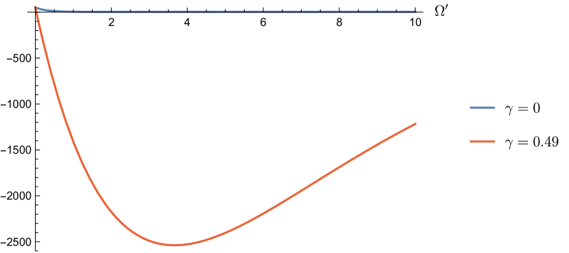
(b)

Figure 2: Dependence of $V_{\gamma,\nu}+\gamma^{2}\tilde{V}$ on $\gamma$. Four cases are reported, namely for the values $\gamma=0$, i.e. the standard case, $\gamma=0.1$, $\gamma=0.3$, $\gamma=0.49$. This last case is shown also in figure b, compared with the standard case, for clarity. Notice the well for this last case, due to the predominance of $\gamma^{2}\tilde{V}$ over $V_{\gamma,\nu}$.

For the same reason, the position of the local minimum of the potential shifts with $\gamma$. It is given by the expression

$$\Omega^{\prime}_{\mathrm{min}}=\frac{\sqrt{3}\left[1-2W\left(-\frac{\sqrt{e}\left(1-4\gamma^{2}\right)}{96\gamma^{2}}\right)\right]}{12\left(1-4\gamma^{2}\right)},$$ (22)

where $W(z)$ is the Lambert $W$ function, solution of the equation $z=we^{w}$ with respect to the variable $w$. This function admits real values only for $z>-\frac{1}{e}$. This motivates the bound $\gamma>\frac{1}{2}\sqrt{\frac{e^{3/2}}{24+e^{3/2}}}$, as observed also in Fig. 3.

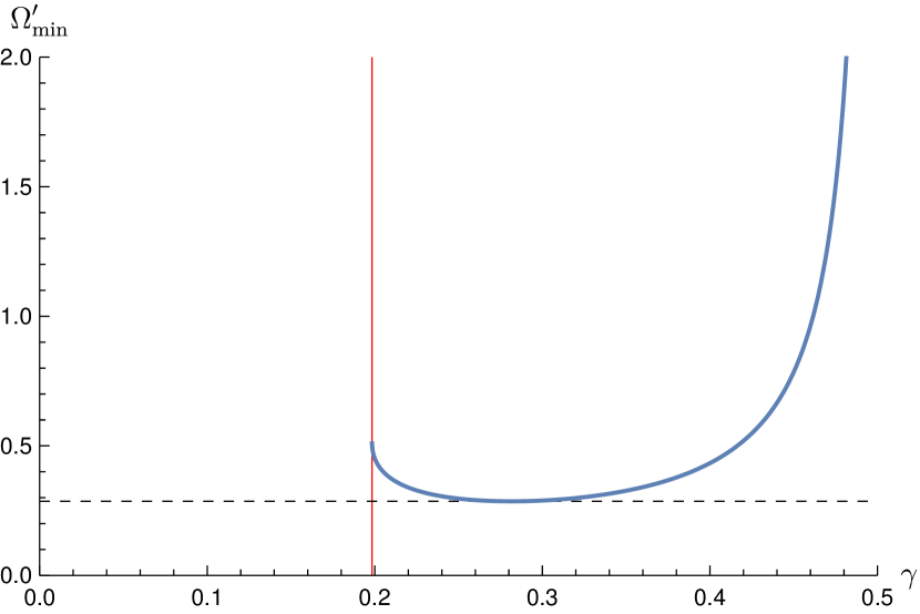
Figure 3: Value of $\Omega^{\prime}_{\mathrm{min}}$ with respect to $\gamma$. The horizontal line, $\Omega_{\mathrm{min}}\simeq 0.28597$, corresponds to the smallest value for $\Omega_{\mathrm{min}}$. The vertical line correspond to the bound $\gamma=\frac{1}{2}\sqrt{\frac{e^{3/2}}{24+e^{3/2}}}$, related with the appearance of the well in Eq. (20). The asymptote at $\gamma=1/2$ is due to the factor $1-4\gamma^{2}$ in Eq. (22).

III Harmonic Oscillator Approximation

It is worth now to investigate further on the behavior of the solution of Eq. (20) in the well described above, that is for $\gamma>\frac{1}{2}\sqrt{\frac{e^{3/2}}{24+e^{3/2}}}$. To do this, let us consider an expansion of the the potential about $\Omega^{\prime}_{\mathrm{min}}$ up to second order. In this case, with the substitution $y=\Omega^{\prime}-\Omega^{\prime}_{\mathrm{min}}$, we find an equation that clearly resembles that of a harmonic oscillator

$$\left\{-\frac{\mathrm{d}^{2}}{\mathrm{d}y^{2}}-b+ay^{2}\right\}\chi(y)=0,$$ (23)

with

$$a= 3(1-4\gamma^{2})^{3}\frac{\left[W\left(-\frac{\sqrt{e}(1-4\gamma^{2})}{96\gamma^{2}}\right)+1\right]}{\gamma^{2}W^{2}\left(-\frac{\sqrt{e}(1-4\gamma^{2})}{96\gamma^{2}}\right)},$$ (24a)

$$b= -3\left[\nu^{2}-\frac{1-4\gamma^{2}}{12\gamma^{2}W\left(-\frac{\sqrt{e}(1-4\gamma^{2})}{96\gamma^{2}}\right)}\right.$$ (24b)

$$\left.-\frac{1-4\gamma^{2}}{24\gamma^{2}W^{2}\left(-\frac{\sqrt{e}(1-4\gamma^{2})}{96\gamma^{2}}\right)}\right],$$ (24c)

where $b$ has the role of an energy. Notice that this analogy is more appropriate the smaller $b$ is, as long as it is positive. In other words, we require $b>0$ to obtain a bound state or, in terms of $\nu$,

$$|\nu|<-\frac{\sqrt{(1-4\gamma^{2})\left[12W\left(-\frac{\sqrt{e}(1-4\gamma^{2})}{96\gamma^{2}}\right)+6\right]}}{12\gamma W\left(-\frac{\sqrt{e}(1-4\gamma^{2})}{96\gamma^{2}}\right)}.$$ (25)

Notice that the rhs is not necessarily real. To obtain a real value for $\nu$, we need to impose the following further condition on $\gamma$

$$\gamma\geq\frac{1}{2}\sqrt{\frac{e}{12+e}}.$$ (26)

Furthermore, this value for $\gamma$ is greater than the minimal value necessary to form a well in the potential.

Continuing in this analogy, and using the following redefinitions

$$E= \frac{b}{2}, \omega= \sqrt{a},$$ (27)

and, furthermore, considering an harmonic oscillator with $\hbar=m=1$, we have the following relation for the energy levels

$$E=\omega\left(n+\frac{1}{2}\right)\qquad\Rightarrow\qquad b=\sqrt{a}(2n+1),\qquad n\in\mathbb{N}.$$ (28)

This relation imposes a quantization rule for the parameter $\nu$ for a given value of $\gamma$

$$\nu=\frac{\sqrt{1-4\gamma^{2}}}{2\sqrt{6}}\left\{\frac{2W\left(-\frac{\sqrt{e}(1-4\gamma^{2})}{96\gamma^{2}}\right)+1}{\gamma^{2}W^{2}\left(-\frac{\sqrt{e}(1-4\gamma^{2})}{96\gamma^{2}}\right)}\right.\\ \left.+8\sqrt{3}(2n+1)\frac{\sqrt{(1-4\gamma^{2})\left[W\left(-\frac{\sqrt{e}(1-4\gamma^{2})}{96\gamma^{2}}\right)+1\right]}}{\gamma W\left(-\frac{\sqrt{e}(1-4\gamma^{2})}{96\gamma^{2}}\right)}\right\}^{1/2}.$$ (29)

Also in this case, looking for real values of $\nu$ gives constraints on $\gamma$ and the number of possible bounds states, as seen in Fig. 4.

Figure 4: Argument of the square root in Eq. (29) for several values of $n$. The vertical line corresponds to the value $\gamma=\frac{1}{2}\sqrt{\frac{e^{3/2}}{24+e^{3/2}}}$, while the dashed line corresponds to $\gamma=\frac{1}{2}\sqrt{\frac{e}{12+e}}$. Notice that, for large $n$, the square root is real only for values $\gamma\rightarrow 1/2$. In other words, for values of $\gamma$ approaching 1/2, arbitrarily large numbers of bound states are allowed.

Numerically, one finds that a first bound state is allowed for $\gamma>0.268593$, two bound states appear when $\gamma>0.343239$, three for $\gamma>0.379114$, and so forth. In general, a larger number of bound states are allowed for larger values of $\gamma$, provided that $\gamma<1/2$. In the limit $\gamma\rightarrow 1/2$, an infinite ladder of bound states is present.

Perturbing the Approximation

For a better study of the effects of the proposed quantization rule, we will retain terms up to fourth order in $\Omega^{\prime}$ in Eq. (20). Using the same substitution above, we can write

$$\left\{-\frac{\mathrm{d}^{2}}{\mathrm{d}y^{2}}-b+ay^{2}+cy^{3}+dy^{4}\right\}\chi(y)=0,$$ (30)

with

$$c= -2\sqrt{3}(1-4\gamma^{2})^{4}\frac{\left[3W\left(-\frac{\sqrt{e}(1-4\gamma^{2})}{96\gamma^{2}}\right)+4\right]}{\gamma^{2}W^{2}\left(-\frac{\sqrt{e}(1-4\gamma^{2})}{96\gamma^{2}}\right)},$$ (31a)

$$d= 3(1-4\gamma^{2})^{5}\frac{\left[7W\left(-\frac{\sqrt{e}(1-4\gamma^{2})}{96\gamma^{2}}\right)+12\right]}{\gamma^{2}W^{2}\left(-\frac{\sqrt{e}(1-4\gamma^{2})}{96\gamma^{2}}\right)}.$$ (31b)

When these extra terms are small compared to the one already analyzed, one can use perturbation theory to compute the correction to the energy levels.

In general, when $n$ bound states are allowed, the energy of the $n$-th state will be corrected by a term

$$\epsilon_{n,(1)}=\frac{6n^{2}+6n+3}{4}(1-4\gamma^{2})^{2}\frac{7W\left(-\frac{\sqrt{e}(1-4\gamma^{2})}{96\gamma^{2}}\right)+12}{W\left(-\frac{\sqrt{e}(1-4\gamma^{2})}{96\gamma^{2}}\right)+1}.$$ (32)

Notice that, for $\sqrt{\frac{e^{3/2}}{24+e^{3/2}}}<2\gamma<1$, these corrections are always positive and their magnitude increase quadratically with the occupation number $n$, as shown in Fig. 5.

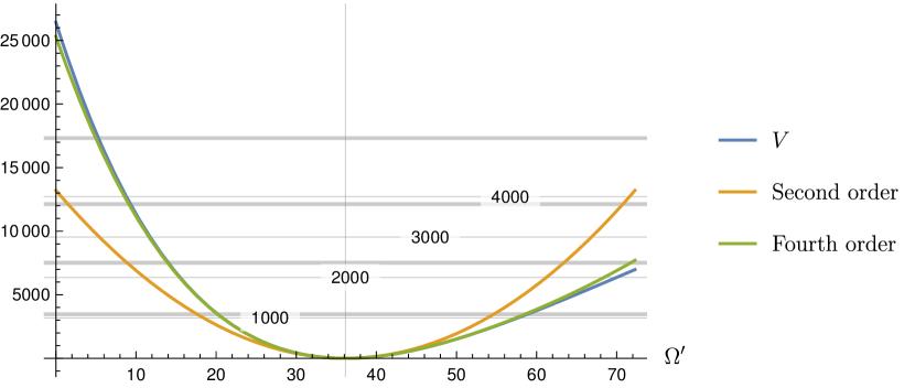
Figure 5: Energies and corresponding corrections to bound states described by Eqs. (23) and (30) for $\gamma=0.449$. Horizontal lines describe the energy levels for 4 particular values of the occupation number (indicated on the plot.) Thin lines correspond to the energy as computed via Eq. (27), while thicker lines are the corrected energy, considering the term in Eq. (32). Finally, in the plot, the blue line corresponds to the full potential in Eq. (20), the orange line correspond to the second order expansion in $\Omega^{\prime}$ about $\Omega^{\prime}_{\mathrm{min}}$, and the green one is the fourth order expansion.

Moreover, in general, if $n$ bound states are allowed, the correction to the $m$-th state is

$$|\eta_{m,(1)}\rangle=\sum_{\begin{subarray}{c}s=0\\ s\neq m\end{subarray}}^{n}\frac{\langle s|cx^{3}+dx^{4}|m\rangle}{E_{m}-E_{s}}=\sum_{u=-\left\lfloor\frac{m+1}{2}\right\rfloor}^{\left\lfloor\frac{n-m-1}{2}\right\rfloor}c\frac{\langle m+2u+1|x^{3}|m\rangle}{E_{m}-E_{m+2u+1}}|m+2u+1\rangle+\sum_{\begin{subarray}{c}v=-\left\lfloor\frac{m}{2}\right\rfloor\\ v\neq 0\end{subarray}}^{\left\lfloor\frac{n-m}{2}\right\rfloor}d\frac{\langle m+2v|x^{4}|m\rangle}{E_{m}-E_{m+2v}}|m+2v\rangle\\ =(1-4\gamma^{2})^{3/4}\frac{\left[3W\left(-\frac{\sqrt{e}(1-4\gamma^{2})}{96\gamma^{2}}\right)+4\right]\sqrt{\gamma W\left(-\frac{\sqrt{e}(1-4\gamma^{2})}{96\gamma^{2}}\right)}}{3^{3/4}\sqrt{2}\left[W\left(-\frac{\sqrt{e}(1-4\gamma^{2})}{96\gamma^{2}}\right)+1\right]^{5/4}}\\ \times\left[-\frac{\sqrt{m^{\underline{3}}}}{3}|m-3\rangle-3m^{3/2}|m-1\rangle+3(m+1)^{3/2}|m+1\rangle+\frac{\sqrt{(m+1)^{\overline{3}}}}{3}|m+3\rangle\right]\\ -(1-4\gamma^{2})^{2}\frac{\left[7W\left(-\frac{\sqrt{e}(1-4\gamma^{2})}{96\gamma^{2}}\right)+12\right]\gamma W\left(-\frac{\sqrt{e}(1-4\gamma^{2})}{96\gamma^{2}}\right)}{8\sqrt{3}\left[W\left(-\frac{\sqrt{e}(1-4\gamma^{2})}{96\gamma^{2}}\right)+1\right]^{3/2}}\\ \times\left[-\frac{\sqrt{m^{\underline{4}}}}{2}|m-4\rangle-2\sqrt{m^{\underline{2}}}(2m-2+1)|m-2\rangle+2\sqrt{(m+1)^{\overline{2}}}|m+2\rangle+\frac{\sqrt{(m+1)^{\overline{4}}}}{2}|m+4\rangle\right].$$ (33)

IV Conclusion and Outlook

Summarizing what has been found in this work, we have considered the Kantowski-Sachs model in the context of quantum cosmology with a modified quantization rule. In doing so, one of the most interesting results is that, for $\gamma\ll 1/2$ but $\gamma\geq\frac{1}{2}\sqrt{\frac{e^{3/2}}{24+e^{3/2}}}$, this modification has a deep impact only on a relatively restricted region of the coordinate space. Furthermore, it is interesting to observe that this region, for a wide range of values of $\gamma$, is very close to or includes the most probable value for the variable $\Omega$ as found in Garcia-Compean2002 . Therefore, it has a concrete influence on the considered model. Furthermore, we have noticed that, for a particular interval of the modification parameter, a well appears in the quantum potential characterizing the system. The presence of this well is a completely novel aspect of the application of this modification with respect to the standard quantum analysis of the Kantowski-Sachs minisuperspace model. Because of this feature, the solution in that particular region and for given values of the parameter $\gamma$ can be expressed in terms of harmonic oscillator states, the number of which depends on $\gamma$ itself.

The importance of these results goes well beyond the cosmological aspects of Kantowski-Sachs model. In fact, as mentioned above, this model would represent a possible quantum description of a spherically symmetric black hole Gambini2015 . Therefore, continuing the works in Obregon2001 ; Arraut2009 ; Bargueno2015 , it would be possible to use the results presented in this paper to further study these effects on quantum black hole models. In particular, the application of GUP in this context results in a minimal uncertainty for $\Omega$. In turn, it would result in a minimal uncertainty for the radial coordinate of the black hole. This and further analyses will be pursued in future works.

References

- (1) L. J. Garay, “Quantum gravity and minimum length,” International Journal of Modern Physics A 10 no. 02, (Jan, 1995) 145–165, arXiv:9403008 [gr-qc].
- (2) D. J. Gross and P. F. Mende, “String theory beyond the Planck scale,” Nuclear Physics B 303 no. 3, (Jul, 1988) 407–454.
- (3) D. Amati, M. Ciafaloni, and G. Veneziano, “Can spacetime be probed below the string size?,” Physics Letters B 216 no. 1-2, (Jan, 1989) 41–47.
- (4) C. Rovelli and L. Smolin, “Discreteness of area and volume in quantum gravity,” Nuclear Physics B 442 no. 3, (Nov, 1994) 593–619, arXiv:9411005 [gr-qc].
- (5) C. Rovelli, “Loop Quantum Gravity,” Living Reviews in Relativity 1 no. 1, (Dec, 1998) arXiv:gr-qc/9710008.
- (6) A. Ashtekar and J. Pullin, Loop Quantum Gravity, vol. 4 of 100 Years of General Relativity. World Scientific Publishing Company, May, 2017.
- (7) M. Maggiore, “A generalized uncertainty principle in quantum gravity,” Physics Letters B 304 no. 1-2, (Apr, 1993) 65–69, arXiv:9301067 [hep-th].
- (8) F. Scardigli, “Generalized uncertainty principle in quantum gravity from micro-black hole gedanken experiment,” Physics Letters B 452 no. 1-2, (Apr, 1999) 39–44, arXiv:9904025 [hep-th].
- (9) F. Scardigli, R. Casadio “Uncertainty relations and precession of perihelion,” Journal of Physics: Conference Series 701, (2016) 012016.
- (10) F. Scardigli, G. Lambiase, E. Vagenas, “GUP parameter from quantum corrections to the Newtonian potential” Physics Letters B 767 (2016) 242–246, arXiv:1611.01469.
- (11) P. Bosso, S. Das, I. Pikovski, M. Vanner, “Amplified transduction of Planck-scale effects using quantum optics” Physical Review A 96 no. 2 (2017) 023849, arXiv:1610.06796.
- (12) G. Lambiase, F. Scardigli, “Lorentz violation and generalized uncertainty principle” Physical Review D 97 no. 7 (2018) 075003, arXiv:1709.00637.
- (13) P. Bosso, S. Das, R. Mann, “Potential tests of the generalized uncertainty principle in the advanced LIGO experiment,” Physics Letters B 785 (2018) 498-505, arXiv:1804.03620.
- (14) F. Scardigli, M. Blasone, G. Luciano, and R. Casadio, “Modified Unruh effect from Generalized Uncertainty Principle,” The European Physical Journal C 78 no. 9 (2018) 728, arXiv:1804.05282.
- (15) T. Kanazawa, G. Lambiase, G. Vilasi, A. Yoshioka, “Noncommutative Schwarzschild geometry and generalized uncertainty principle,” The European Physical Journal C 79 no. 2 (2019) 95.
- (16) L. Buoninfante, G.C. Luciano, L. Petruzziello, “Generalized Uncertainty Principle and Corpuscular Gravity,” The European Physical Journal C 79 no. 8 (2019) 663, arXiv:1903.01382.
- (17) P. A. Bushev, et al., “Testing the generalized uncertainty principle with macroscopic mechanical oscillators and pendulums,” Physical Review D 100 no. 6 (2019) 066020, arXiv:1903.03346.
- (18) A. Kempf, G. Mangano, and R. B. Mann, “Hilbert space representation of the minimal length uncertainty relation,” Physical Review D 52 no. 2, (Jul, 1995) 1108–1118, arXiv:9412167 [hep-th].
- (19) S. Das and E. C. Vagenas, “Phenomenological Implications of the Generalized Uncertainty Principle,” Canadian Journal of Physics 87 no. 3, (Jan, 2009) 233–240, arXiv:0901.1768.
- (20) P. Bosso, “Generalized Uncertainty Principle and Quantum Gravity Phenomenology,” Ph.D. Thesis, University of Lethbridge, (Aug, 2017), arXiv:1709.04947
- (21) P. Bosso, “Rigorous Hamiltonian and Lagrangian analysis of classical and quantum theories with minimal length,” Physical Review D 97 no. 12, (Apr, 2018) 126010, arXiv:1804.08202.
- (22) M. Ryan, Hamiltonian Cosmology, vol. 13 of Lecture Notes in Physics. Springer Berlin Heidelberg, Berlin, Heidelberg, 1972.
- (23) J. B. Hartle and S. W. Hawking, “Wave function of the Universe,” Physical Review D 28 no. 12, (Dec, 1983) 2960–2975.
- (24) M. Ryan and L. Shepley, Homogeneous Relativistic Cosmologies. Princeton University Press, 2015.
- (25) A. Ashtekar and P. Singh, “Loop quantum cosmology: a status report,” Classical and Quantum Gravity 28 no. 21, (Nov, 2011) 213001, arXiv:1108.0893 [gr-qc].
- (26) I. Agullo and P. Singh, “Loop Quantum Cosmology,” in Loop Quantum Gravity, A. Ashtekar and J. Pullin, eds., ch. 6, pp. 183–240. World Scientific Publishing Company, May, 2017. arXiv:1612.01236.
- (27) H. Bergeron, E. Czuchry, and P. Małkiewicz, Coherent states quantization and affinesymmetry in quantum models of gravitationalsingularities, vol. 205 of Springer Proceedings in Physics. Springer, Cham, 2018, arXiv:1708.09670.
- (28) H. García-Compeán, O. Obregón, and C. Ramírez, “Noncommutative quantum cosmology.,” Physical review letters 88 no. 16, (Apr, 2002) 161301, arXiv:0107250 [hep-th].
- (29) M. Aguero, J. A. S. Aguilar, C. Ortiz, M. Sabido, and J. Socorro, “Noncommutative Bianchi Type II Quantum Cosmology,” International Journal of Theoretical Physics 46 no. 11, (Oct, 2007) 2928–2934, arXiv:0703151 [gr-qc].
- (30) H. S. Snyder, “Quantized Space-Time,” Physical Review 71 no. 1, (Jan, 1947) 38–41.
- (31) A. Connes, “Noncommutative geometry and reality,” Journal of Mathematical Physics 36 no. 11, (Nov, 1995) 6194–6231.
- (32) M. Douglas and N. Nekrasov, “Noncommutative field theory,” Reviews of Modern Physics 73 no. 4, (Nov, 2001) 977–1029, arXiv:0106048 [hep-th].
- (33) C. W. Misner, “Quantum Cosmology. I,” Physical Review 186 no. 5, (Oct, 1969) 1319–1327.
- (34) C. W. Misner, Minisuperspace. W. H. Freeman, San Francisco, 1972.
- (35) M. Kober, “Generalized Quantization Principle in Canonical Quantum Gravity and Application to Quantum Cosmology,” Int.J.Mod.Phys. A 27, 1250106 (2011) arXiv:1109.4629
- (36) M. Faizal, “Deformation of the Wheeler-DeWitt Equation,” Int.J.Mod.Phys. A 29, 1450106 (2014) arXiv:1406.0273
- (37) R. Garattini and M. Faizal, “Cosmological constant from a deformation of the Wheeler–DeWitt equation,” Nucl.Phys. B 905, 313–326 (2016) arXiv:1510.04423
- (38) O. Obregón and M. P. Ryan, “Quantum Planck size blackhole states without a horizon,” Modern Physics Letters A 13 no. 40, (Dec, 1998) 3251–3258.
- (39) R. Gambini and J. Pullin, “An introduction to spherically symmetric loop quantum gravity black holes,” vol. 1647, pp. 19–22. 2015.
- (40) O. Obregón, M. Sabido, and V. I. Tkach, “Entropy Using Path Integrals for Quantum Black Hole Models,” General Relativity and Gravitation 33 no. 5, (May, 2001) 913–919, arXiv:0003023 [gr-qc].
- (41) I. Arraut, D. Batic, and M. Nowakowski, “Comparing two approaches to Hawking radiation of Schwarzschild-de Sitter black holes,” Class.Quant.Grav. 26, 125006 (2009) arXiv:0810.5156
- (42) P. Bargueño and E. C. Vagenas, “Semiclassical corrections to black hole entropy and the generalized uncertainty principle,” Physics Letters, Section B: Nuclear, Elementary Particle and High-Energy Physics 742 (2015) 15–18, arXiv:1501.03256.