Data-Optimized Coronal Field Model:
I. Proof of concept

Abstract

Deriving the strength and direction of the three-dimensional (3D) magnetic field in the solar atmosphere is fundamental for understanding its dynamics. Volume information on the magnetic field mostly relies on coupling 3D reconstruction methods with photospheric and/or chromospheric surface vector magnetic fields. Infrared coronal polarimetry could provide additional information to better constrain magnetic field reconstructions. However, combining such data with reconstruction methods is challenging, e.g., because of the optical-thinness of the solar corona and the lack and limitations of stereoscopic polarimetry. To address these issues, we introduce the Data-Optimized Coronal Field Model (DOCFM) framework, a model-data fitting approach that combines a parametrized 3D generative model, e.g., a magnetic field extrapolation or a magnetohydrodynamic model, with forward modeling of coronal data. We test it with a parametrized flux rope insertion method and infrared coronal polarimetry where synthetic observations are created from a known “ground truth” physical state. We show that this framework allows us to accurately retrieve the ground truth 3D magnetic field of a set of force-free field solutions from the flux rope insertion method. In observational studies, the DOCFM will provide a means to force the solutions derived with different reconstruction methods to satisfy additional, common, coronal constraints. The DOCFM framework therefore opens new perspectives for the exploitation of coronal polarimetry in magnetic field reconstructions and for developing new techniques to more reliably infer the 3D magnetic fields that trigger solar flares and coronal mass ejections.

1. Introduction

Solar flares and coronal mass ejections (CMEs) are driven by the evolution of current-carrying magnetic fields in the solar corona (e.g., Forbes00; Priest03; Schrijver05; Shibata11; Aulanier12). Deriving the three-dimensional (3D) properties of such non-potential magnetic fields is critical for identifying the mechanism(s) driving flares and CMEs, as well as for understanding and predicting their evolution (e.g., Bateman78; Hood81; Antiochos99; Kusano12; Pariat17). Hence, measuring the strength and direction of the 3D magnetic field in the solar coronal volume is fundamental.

Magnetic field information in the solar corona is mostly derived from the inversion of off-limb polarization measurements associated with the Zeeman and Hanle effects (e.g., Harvey69; Casini99; Lin04; Centeno10). The Zeeman effect creates a frequency-modulated polarization signal sensitive to both the strength and direction of the magnetic field. Due to the large Doppler widths of coronal emission lines and the wavelength squared scaling, the Zeeman effect in the corona is better observed with infrared (IR) spectral lines (e.g., Judge98; Penn14). However, the coronal magnetic field is weak, with typical values of 1 to 10 Gauss, except right above solar active regions where it can reach up to a few 100 Gauss (e.g., Kuhn96; Lin00). The corresponding fraction of circular polarization in IR lines, such as the Fe XIII lines, is thus only expected to be of the order of $10^{-4}$ (equivalent to a 1 Gauss magnetic field strength; e.g., Querfeld82; Plowman14). Accurately measuring the Zeeman-induced polarization signal in the corona is therefore a challenging task that will require large aperture telescopes, such as the Large Coronagraph (1.5 meter) on the COronal Solar Magnetism Observatory (COSMO; Tomczyk16) or the 4-meter Daniel K. Inouye Solar Telescope (DKIST; see Keil11, and references therein).

The Hanle effect is the second main mechanism exploited for diagnosing the solar coronal magnetic field. This process modifies the polarization of spectral lines in the presence of a magnetic field (e.g., Hanle24; SahalBrechot77; Bommier82; Arnaud87). As opposed to the Zeeman effect, the Hanle effect is a depolarization mechanism. It therefore requires the prior existence of polarization by means of other physical processes such as, e.g., radiation scattering (e.g., Charvin65). Sensitivity of the Hanle effect to the magnetic field can range from a few milli-Gauss to several hundred Gauss depending on the choice of spectral line and the strength and direction of the magnetic field (e.g., Bommier82; Raouafi16). The Hanle effect is hence a powerful tool for probing the coronal magnetic field, as confirmed by theoretical (e.g., Judge06; Rachmeler13; Rachmeler14; Dalmasse16) and observational (e.g., BakSteslicka13; Morton16; Gibson17; KarnaSub) studies with, e.g., off-limb coronal polarimetry in the IR Fe XIII lines. Note, though, that routine measurements of coronal polarization are currently limited to the IR Fe XIII lines with the Coronal Multi-channel Polarimeter (CoMP; Tomczyk08) for which the Hanle effect operates in the saturated regime (e.g., Casini99). In practice, it means that the measured linear polarization is sensitive to the magnetic field direction but not its strength. Coronal polarimetry with other spectral lines, such as the IR He I 10830 Å or the UV H I Ly $\alpha$ lines, will be necessary to further obtain Hanle diagnostics sensitive to the coronal magnetic field strength (e.g., Raouafi16).

While the Zeeman and Hanle effects offer powerful diagnostics of the coronal magnetic field, determining the actual 3D coronal magnetic field from coronal polarimetry remains a true challenge. In addition to the previously discussed limitations, the solar corona is optically thin at most wavelengths. It follows that the measured polarization signal is the integration of all the plasma emission along the line of sight (LOS). Consequently, it is in general not possible to invert the polarization maps into 2D maps of the magnetic field. Furthermore, it is difficult to extract individual magnetic field data at specific positions along the LOS, even with stereoscopic measurements whether used on their own or combined with 3D magnetic field extrapolation methods (e.g., Kramar13; Kramar16). In particular, one of the main challenges with stereoscopic polarimetry relies on the limited amount of information that can be retrieved from the data, either due to a limited range in magnetic strength sensitivity at a given wavelength, or the lack of it for, e.g., the linear polarization signal measured for the Fe XIII lines. The latter is only sensitive to the magnetic field direction and further possesses both a $90^{\circ}$ and $180^{\circ}$ ambiguity (saturated regime of the Hanle effect; Judge07; Plowman14).

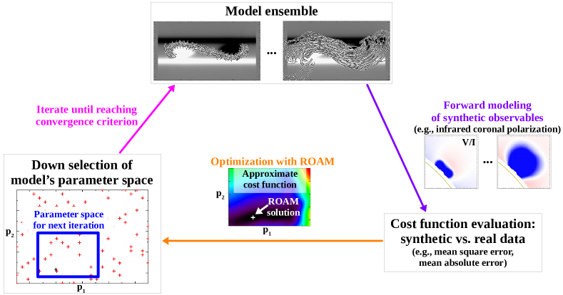
Figure 1.— General sketch of the DOCFM framework.

Volume information on the vector magnetic field in the solar corona thus mostly relies on the approximate 3D solution obtained by coupling surface magnetic field maps (so-called vector magnetograms), derived from photospheric and/or chromospheric polarimetry, with 3D magnetic field reconstruction methods. 3D techniques for reconstructing the solar coronal magnetic field from surface measurements are either of the nonlinear force-free field (NLFFF; e.g., vanBallegooijen04; Wheatland07; Wiegelmann10; Valori10; Contopoulos11; Malanushenko12; Amari13; Yeates14) or the magnetohydrodynamics (MHD; e.g., Mikic99; Inoue11; Feng12; Zhu13) type.

These reconstruction methods differ by the equations solved, the implemented algorithms, and their treatment of the vector magnetograms as boundary conditions (e.g., full vs. LOS vector, pre-processing to create more force-free boundary conditions). As a consequence, the 3D, current-carrying, magnetic field solution and its properties can strongly vary from one method to the other. For instance, DeRosa09, DeRosa15 and Yeates18 reported variations between reconstruction methods that can reach up to 200$\%$ for the ratio of free to potential magnetic energy, as well as for relative magnetic helicity, which are key ingredients for producing solar flares and CMEs (e.g., Low96; Forbes06; Tziotziou12; Zuccarello18). Even the magnetic topology, which can also play a key role on the stability of the 3D magnetic field configuration (e.g., Gorbachev89; Somov93; Savcheva16), can be strongly affected by the choice of reconstruction method. This can make it difficult to determine the role of magnetic topology in the triggering of solar flares, in particular for events for which some reconstruction methods may produce a flux rope prior to the flare (e.g., Amari18) when others only produce sheared arcades (e.g., Jiang16).

The present paper is the first in a series that investigates the possibility of improving the reliability of 3D magnetic field reconstructions by further exploiting coronal polarimetry. The methodology we propose and the tools we use are described in Section 2. Section 3 presents the test-case for which we test and prove the concept of our approach, using a known “ground truth” 3D magnetic field to create synthetic observations. The results of our analysis are reported in Section 4. Section LABEL:sec:S-Discussion discusses the applicability, limitations and perspectives of our approach. Our conclusions are summarized in Section LABEL:sec:S-Conclusions.

2. Method

2.1. Summary of approach

The general framework we propose to couple existing 3D magnetic field reconstructions with coronal polarimetric observations is the Data-Optimized Coronal Field Model (DOCFM). It is a model-data fitting approach of the 3D reconstruction of the coronal magnetic field. The DOCFM is built on the three following general bases:

1. A generative 3D magnetic field model (i.e., extrapolation/reconstruction) parametrized through its electric currents. This can be done either at the photospheric boundary (e.g., by means of the transverse magnetic field or the force-free parameter) or in the volume (e.g., for flux rope insertion methods; e.g., vanBallegooijen04; Titov14; Titov18). The generative model then creates the physical state of the corona (e.g., magnetic field, plasma pressure, density, temperature).

2. Forward modeling of coronal polarimetry, in particular to address the fact that the solar corona is optically thin and the lack and limitations of stereoscopic coronal polarimetry.

3. Finding the set of parameters that minimize a cost function (or maximize a likelihood function as in Dalmasse16), here the mean squared error between the polarization signal predicted for the magnetic field model and the real polarization data.

LABEL:Fig-DOCFM-diagram presents a general chart of the DOCFM approach.

Previous work has demonstrated the sensitivity of polarization signals in coronal cavities to the 3D magnetic field geometry (e.g., Judge06; BakSteslicka13; Rachmeler13; Rachmeler14). Our main focus is thus on exploiting coronal cavities and their IR polarimetric signatures as observed by CoMP to constrain the 3D magnetic field that precedes CMEs. The parametrized 3D magnetic field model we choose to work with is the flux rope insertion method of vanBallegooijen04 briefly presented in Section 2.2. This method uses the LOS measurement of the photospheric magnetic field and an analytical model to produce a coronal flux rope. It is particularly useful for studying coronal cavities, which are likely associated with 3D magnetic flux ropes in weak field regions where the LOS magnetic field is still well-enough above the noise level while the transverse field is not. The flux rope insertion method is thus better suited for studying such structures than more traditional extrapolation techniques for which flux ropes arise from the electric currents associated with the photospheric transverse magnetic field measurements, and which would likely fail to retrieve the flux ropes when such measurements are too noisy. Our choice of synthetic coronal polarimetric data is IR polarimetry in the 10747 Å Fe XIII-I line, synthesized with the codes of the FORWARD IDL package (see Section 2.3; Gibson16). For the minimization, we use an iterative implementation of the Radial-basis-functions Optimization Approximation Method (Dalmasse16) described in Section 2.4.

2.2. Generative magnetic field model

In the the strong field regions of the solar corona, the plasma $\beta$, i.e., the ratio of plasma pressure to magnetic pressure, is relatively low (about $10^{-4}$ to $10^{-2}$; e.g., Gary01). In this low-$\beta$ environment, all non-magnetic forces (e.g., kinematic plasma flow pressure, gravity) are dominated by the magnetic ones and can thus be neglected. As a consequence, the Lorentz force vanishes (i.e., the magnetic pressure force is compensated by the magnetic tension force) and the coronal magnetic field can be modeled as a force-free field, such that

$$\nabla\times{\mathbf{B}}(r)=\frac{4\pi}{c}{\mathbf{j}}(r)=\alpha(r){\mathbf{B}}(r)\,,$$ (1)

where $c$ is the speed of light, ${\mathbf{B}}(r)$ is the vector magnetic field, ${\mathbf{j}}(r)$ is the electric current density and $\alpha(r)$ is the force-free parameter. $\alpha(r)=0$ refers to the potential field solution, while constant-$\alpha$ solutions are the so-called linear force-free fields (e.g., Alissandrakis81). In the most general case, $\alpha(r)$ is constant along individual magnetic field lines, but varies from one field line to the other, which corresponds to the NLFFF solutions (see, e.g., review by Wiegelmann12R).

Several NLFFF methods have been developed to solve for Equation (1) and extrapolate, or reconstruct, the 3D coronal magnetic field from 2D photospheric magnetic field measurements as a bottom boundary condition (see, e.g., Grad58; Amari06; Wheatland07; Valori10; Inoue12; Malanushenko12; Wiegelmann12; Titov18, to cite a few). In this paper, we use the flux rope insertion method of vanBallegooijen04. Such a choice is motivated by the fact that (1) our main focus is on applying the DOCFM approach to coronal cavities, which are density-depleted regions likely associated with a 3D magnetic flux rope (e.g., BakSteslicka13; Gibson15), and (2) the flux rope insertion method is already a parametrized 3D generative model. The flux rope possesses two parameters, which are the axial flux (i.e., the magnetic flux along the flux rope axis), $\Phi$, and the poloidal flux per unit length (i.e., the magnetic flux per unit length in the direction perpendicular to the flux rope axis), F.

To apply the flux rope insertion method (vanBallegooijen04), a potential field source surface (PFSS) extrapolation is first computed from LOS photospheric magnetograms. EUV data of, e.g., solar filaments (see, e.g., Su11; Savcheva12), are then used to determine the photospheric feet and path of the flux rope. A field-free (i.e., zero-magnetic field), 3D thin channel is created along the flux rope path in the potential field. The parametrized 3D flux rope is then inserted into that field-free thin channel, thus producing a magnetic field configuration containing a flux rope, but which is out of equilibrium. The magnetic field is then driven towards a quasi-force-free state by means of magnetofrictional relaxation (more details on the flux rope insertion method can be found in, e.g., vanBallegooijen04; Bobra08; Savcheva16). The entire flux rope insertion procedure is performed in terms of modifying and evolving the vector potential, ${\mathbf{A}}$ (defined by ${\mathbf{B}}=\nabla\times{\mathbf{A}}$), through the induction equation and using hyperdiffusion to smooth gradients in the force-free parameter (Yang86; vanBallegooijen00). The advantage of performing the relaxation with the vector potential is that it automatically ensures that the solenoidal condition for the magnetic field (i.e., $\nabla\cdot{\mathbf{B}}=0$) is numerically satisfied.

For all flux rope insertions produced in this paper, the magnetofrictional relaxation is applied without any diffusion for the first 100 steps. Then, hyperdiffusion is used until $6\times 10^{4}$ relaxation steps have been performed, at which point the relaxation is stopped and stable NLFFF models are obtained.

2.3. Forward modeling of coronal polarimetry

As mentioned Section 1, the solar corona is optically thin and stereoscopic observations of the coronal polarization are currently not available. In addition, the linear polarization measured in the Fe XIII lines is sensitive to the direction of the coronal magnetic field but not its strength. Hence, off-limb coronal polarimetry as measured by CoMP provides a LOS-integrated signal that cannot be inverted into a 2D plane-of-sky (POS) magnetic field that could be directly plugged in the 3D magnetic field model. To couple such coronal polarimetric data with coronal magnetic field reconstruction models, we must instead rely on a model-data fitting approach. The latter requires a means to produce synthetic coronal observations from a given magnetic field model cube and observing position.

To produce synthetic coronal polarimetric data, we use the FORWARD IDL suite (Gibson16). FORWARD is a package for multiwavelength coronal magnetometry that is integrated into the SolarSoft (Freeland98) IDL toolset. It is designed to create synthetic observables and compare them to coronal data (a full description is provided in Gibson16). In particular, FORWARD employs the Coronal Line Emission (CLE) polarimetry code developed by Casini99 to synthesize full Stokes $(I,Q,U,V)$ line profiles for visible and IR forbidden lines including, but not limited to, the Fe XIII lines routinely observed by the CoMP and used in the analyses performed in this paper. Stokes $I$ corresponds to the integrated total line intensity. Stokes $(Q,U)$ are the two components of the linear polarization. And Stokes $V$ is the circular polarization.

2.4. Optimization of flux-rope parameters

To find the set of parameters minimizing the mean squared error (MSE) between the predicted polarization signal for the magnetic field model and the real data, we use an iterative implementation of the Radial-basis-functions Optimization Approximation Method (ROAM; e.g., Dalmasse16). ROAM relies on evaluating a cost function (hence, the generative magnetic field model and synthetic observables) for a sparse sample of model-parameter values, approximating the sparse cost function sample with a series of radial basis functions (RBF) to obtain an analytical form for the cost function as a function of the model-parameter values, and computing an estimate of the best-fit parameters by minimizing the analytical form of the cost function (the more detailed procedure is provided in Section 2 of Dalmasse16).

The generative magnetic field model we use to test the applicability and accuracy of the DOCFM approach only has two parameters (cf. Section 2.2). ROAM was developed to be a fast and efficient optimization method for higher-dimensional optimization problems, i.e., with a number of parameters at least equal to 3. Thus, in practice, there exists other optimization methods that would be faster and more efficient (i.e., requiring fewer model evaluations) than ROAM for the optimization problem at hand. However, the goal of this paper is to show the applicability of the complete DOCFM framework, which we developed to be general enough to be used with generative magnetic field models having a large number of parameters and for which ROAM is better suited. The latter is the motivation behind the use of ROAM in this investigation.

Let $p$ be the number of (model)-parameters, ${\mathbf{x}}=(x_{1},x_{2},...,x_{p})$ a vector parameter in the $p$-dimensional parameter space, and $S=\{{\mathbf{x}}^{i=\{1,...,n\}}\}$ a random sample of $n$ independent vector parameters (i.e., $x^{j\neq i}_{k}\neq x^{i}_{k}$ for all $k$). As shown by the tests performed in Dalmasse16, the estimate of best-fit parameters obtained with the ROAM can be sensitive to the choice of sample of vector parameters, i.e., to the choice of $S$. On the other hand, the mean best-fit vector parameter obtained by averaging the best-fit vector parameters computed by applying ROAM with different samples, actually provides a good approximation of the true best-fit vector parameter. We use the latter result to build an iterative implementation of ROAM that gives an estimate of the best-fit vector parameters that is quasi-independent of the sample choice. Our iterative application of ROAM is based on adaptive refinement, such that refinement is performed in the region where the best-fit vector parameter is likely to be. The algorithm is as follows:

1. Let $R$ refer to both the refinement level and iteration number, such that $R=0$ corresponds to the un-refined starting grid.

2. Choose boundaries, $((x^{\mathrm{min}}_{1},x^{\mathrm{max}}_{1}),...,(x^{\mathrm{min}}_{p},x^{\mathrm{max}}_{p}))=((x^{\mathrm{min},R=0}_{1},x^{\mathrm{max},R=0}_{1}),...,(x^{\mathrm{min},R=0}_{p},x^{\mathrm{max},R=0}_{p}))$, to define the parameter space region where to search for the parameter values minimizing the MSE.

3. Use latin hypercube sampling (LHS; e.g., McKay79; Iman81) to create 3, randomly chosen, sparse samples, $(S^{R}_{1},S^{R}_{2},S^{R}_{3})$ of $n$ vector parameters for the parameter space region of interest. The 3 samples are chosen with the constraint that the 3$n$ vector parameters are all different.

4. Combine the latin hypercube samples to produce the 7 samples, $(S^{\prime}_{1},S^{\prime}_{2},S^{\prime}_{3},S^{\prime}_{4},S^{\prime}_{5},S^{\prime}_{6},S^{\prime}_{7})=(S^{R}_{1},S^{R}_{2},S^{R}_{3},S^{R}_{1}+S^{R}_{2},S^{R}_{1}+S^{R}_{3},S^{R}_{2}+S^{R}_{3},S^{R}_{1}+S^{R}_{2}+S^{R}_{3})$.

5. Apply ROAM to the 7 samples, $(S^{\prime}_{d=1,...,7})$, to obtain 7 estimates of best-fit vector parameters, $({\mathbf{x}}^{\mathrm{bf},R}(S^{\prime}_{1}),...,{\mathbf{x}}^{\mathrm{bf},R}(S^{\prime}_{7}))$, at the $R$-th iteration.

6. Compute the optimization solution vector defined as the mean best-fit solution, $\mu^{R}=(\mu^{R}_{1},\mu^{R}_{2},...,\mu^{R}_{p})$, and its standard deviation vector, $\sigma^{R}=(\sigma^{R}_{1},\sigma^{R}_{2},...,\sigma^{R}_{p})$, at the $R$-th iteration

   $$\mu^{R}_{k} = \frac{1}{7}\sum^{7}_{d=1}x^{\mathrm{bf},R}_{k}(S^{\prime}_{d})$$ (2)

   $$\sigma^{R}_{k} = \sqrt{\frac{1}{7}\sum^{7}_{d=1}\left(x^{\mathrm{bf},R}_{k}(S^{\prime}_{d})-\mu^{R}_{k}\right)^{2}}\,,$$ (3)

7. Compute the parameter-space boundaries where refinement is needed according to

   $$x^{\mathrm{min},R+1}_{k} = \frac{\left(\lambda-1\right)x^{\mathrm{min},R}_{k}+\min\left(x^{\mathrm{bf}}_{k}(S^{\prime}_{1}),...,x^{\mathrm{bf}}_{k}(S^{\prime}_{7})\right)}{\lambda}$$ (4)

   $$x^{\mathrm{max},R+1}_{k} = \frac{\left(\lambda-1\right)x^{\mathrm{max},R}_{k}+\max\left(x^{\mathrm{bf}}_{k}(S^{\prime}_{1}),...,x^{\mathrm{bf}}_{k}(S^{\prime}_{7})\right)}{\lambda}\,,$$ (5)

   where $\lambda>1$ is the shrinkage coefficient. It is a user-specified scalar that controls the speed at which the refining region shrinks; larger $\lambda$ values lead to slower shrinkage.

8. Repeat steps 3 through 7 for the refined region until a convergence criterion is met (e.g., $\sigma^{R}_{k}$ and/or the refining region are sufficiently small).

3. Test-case

3.1. Ground-truth magnetic fields

Table 1Ground-truth parameter values

Flux rope model	$\Phi_{\mathrm{GT}}$ (Mx)	$\mathrm{F}_{\mathrm{GT}}$ (Mx cm${}^{-1}$)
Low-height Low-twist (LL)	$2.50\times 10^{20}$	$-1.00\times 10^{8}$
Low-height Mild-twist (LM)	$2.50\times 10^{20}$	$-4.00\times 10^{9}$
Low-height High-twist (LH)	$2.50\times 10^{20}$	$-1.00\times 10^{10}$
Mid-height Low-twist (ML)	$5.00\times 10^{20}$	$-1.00\times 10^{8}$
Mid-height Mild-twist (MM)	$5.00\times 10^{20}$	$-4.00\times 10^{9}$
Mid-height High-twist (MH)	$5.00\times 10^{20}$	$-1.00\times 10^{10}$
High-height Low-twist (HL)	$7.50\times 10^{20}$	$-1.00\times 10^{8}$
High-height Mild-twist (HM)	$7.50\times 10^{20}$	$-4.00\times 10^{9}$
High-height High-twist (HH)	$7.50\times 10^{20}$	$-1.00\times 10^{10}$

Note. — Each model is used to produce a set of coronal polarimetric observations to be fitted, as if we were applying the DOCFM to 9 different cavity systems in observational applications. Such a choice allows us to show that the robustness and success of the DOCFM framework are independent of the choice of parameter values for the ground truth 3D magnetic field.

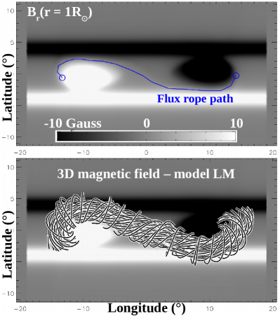
Figure 2.— Top: Photospheric magnetic flux distribution (grey scale) and flux rope path (blue line) and feet (blue circles) used to prove the concept of the DOCFM approach with the flux rope insertion method, as given from Fan12 MHD simulation. The magnetic field is in units of Gauss. Bottom: Top view of selected 3D magnetic field lines for ground-truth model LM which parameter values are reported in Table 1.

With this series of papers, our goal is to investigate the possibility of improving the reliability of 3D magnetic field reconstructions by further exploiting coronal polarimetry. The primary goal of this investigation is to prove the concept of the methodology and characterize the uncertainties that are both inherent to the limited amount of information contained in the polarimetric data (see Section 1) and the limitations of the optimization algorithm (described in Section 2.4). To that end, we begin by creating a “ground truth” solution, which is a full representation of the coronal physical state (magnetic field, density, temperature, pressure) created from a generative model. With this ground truth solution, we can forward model synthetic coronal data that will be used in the place of true observations. The point of such an approach is to test the capability of the DOCFM framework for a problem where the solution is fully known.

Limitations due to the ability of the generative model to reproduce a given magnetic field will be addressed in our second paper in this series (Paper II). For these reasons, the ground-truth magnetic fields we use in this paper are created with the reconstruction model we use, i.e., the flux rope insertion method briefly described in Section 2.2.

To produce a ground-truth magnetic field with the flux rope insertion method, we first need a photospheric magnetic flux distribution and a flux rope path (see Section 2.2). LABEL:Fig-GT-Bfield displays the photospheric magnetogram and flux rope path selected for our investigation. The boundary condition is chosen to be consistent with that of flux-rope MHD model of Fan12, which we will use in Paper II to further test the robustness of our approach. For consistency, we computed the PFSS from the flux distribution displayed in LABEL:Fig-GT-Bfield with the source surface set at $\approx 6R_{\odot}$, which is far enough from the photosphere to allow most of the arcade magnetic field to be closed. To create the ground-truth, current-carrying magnetic field, we then insert a flux rope with axial flux, $\Phi_{\mathrm{GT}}$, and poloidal flux per unit length, $\mathrm{F}_{\mathrm{GT}}$. LABEL:Fig-GT-Bfield displays the ground-truth solution defined by the set of parameters, $\Phi_{\mathrm{GT}}=2.5\times 10^{20}\ \mathrm{Mx}$ and $\mathrm{F}_{\mathrm{GT}}=-4\times 10^{9}\ \mathrm{Mx}\cdot\mathrm{cm}^{-1}$, which produces a low-lying, mildly-twisted, left-handed flux rope referred to as model LM.

To show that the DOCFM approach works regardless of the choice of ground-truth parameters, $\left(\Phi_{\mathrm{GT}},\mathrm{F}_{\mathrm{GT}}\right)$, and validate it, we consider 8 additional ground truth solutions that are reported in Table 1. Each one of the 9 chosen flux ropes is used to create a set of coronal polarimetric observations to be fitted, as if we were applying the DOCFM framework to finding the 3D magnetic field of 9 different solar coronal cavities. In particular, we produce low-height, mid-height and high-height ground truth flux ropes with different degrees of magnetic twist by choosing different axial and poloidal flux values.

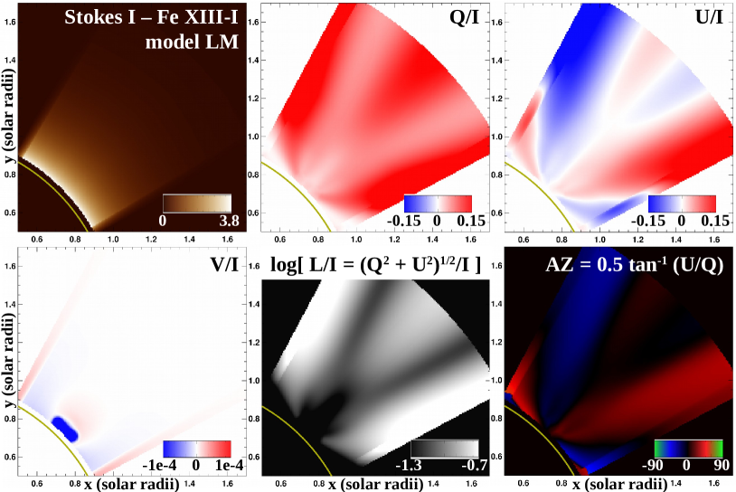
Figure 3.— Coronal polarimetric observations in the Fe XIII-I line synthesized with FORWARD for the ground-truth model LM which parameter values are reported in Table 1. The flux rope axis is aligned with the LOS. The total line intensity (Stokes $I$), the two components of the fraction of linear polarization ($Q/I$ and $U/I$), and the fraction of circular polarization ($V/I$) are displayed together with the fraction of linear ($L/I=\sqrt{Q^{2}+U^{2}}/I$) polarization and the azimuth ($AZ=0.5\tan^{-1}(U/Q)$). Notice the darkening in the central part of the flux rope and the dark lagomorphic shape in the $L/I$ signal, which are typical signatures expected in the $L/I$ signal associated with flux ropes closely aligned with the LOS (e.g., BakSteslicka13; Rachmeler13).

3.2. Synthetic data

Our application of the DOCFM framework has a focus on the exploitation of off-limb coronal polarimetry as obtained by the CoMP instrument in the Fe XIII-I line (10747 Å; Tomczyk08). For our analysis, we use Stokes I, Q, U and V images synthesized with FORWARD (see Section 2.3). We further considered Stokes $L=\sqrt{Q^{2}+U^{2}}$ and Stokes $AZ=0.5\tan^{-1}(U/Q)$ images, which provide an alternate representation of the linear polarization and have been shown to provide useful diagnostics of the coronal magnetic field (e.g., BakSteslicka13; Rachmeler14; Gibson17; KarnaSub). Each synthetic Stokes image is generated with a field of view (FOV) set to $y\times z=[0.5R_{\odot},1.7R_{\odot}]^{2}$ ($y$ and $z$ being the plane-of-sky coordinates) and $x=[-0.79,0.79]R_{\odot}$ in the LOS direction. The POS and the LOS are respectively covered with $192^{2}$ and 161 grid points. The resulting spatial resolution is $\approx 6.0^{\prime\prime}\times 6.0^{\prime\prime}$ in the POS, and $\approx 9.4^{\prime\prime}$ along the LOS. The forward calculations of the Stokes parameters are limited to a radial range of $[1.03,1.7]R_{\odot}$, where 1.03 corresponds to the lower limit of CoMP FOV. Our choice of spatial resolution of $6.0^{\prime\prime}$ is only slightly lower than that of CoMP ($4.5^{\prime\prime}$) to allow us to maintain a relatively low computational time per set of Stokes parameters (about 15 minutes on a Linux workstation with an Intel Xeon E5-2630 v4 processor).

Forward modeling of coronal polarimetric observables requires a 3D magnetic field model and also a plasma model, because the density and temperature are involved in the formation process of any emission line. However, most NLFFF generative models, such as the flux rope insertion one, disregard the plasma and only provide a 3D magnetic field solution. In the DOCFM framework, we therefore need to provide a plasma model if the magnetic field reconstruction model does not include one. For a FFF, the plasma solution compatible with the force-free assumption is a spherically symmetric hydrostatic atmosphere. If we further assume that the atmosphere is isothermal with coronal temperature, $T_{c}$, then the plasma density and pressure are

$$n(r) = n_{c}\exp\left(\frac{R_{c}}{h}\cdot\frac{R_{c}-r}{r}\right)$$ (6)

$$h = \frac{2k_{B}T_{c}R^{2}_{c}}{GM_{c}m_{p}}$$ (7)

$$P(r) = 2n(r)k_{B}T_{c}\,,$$ (8)

where $r$ is the radial distance to the center of the Sun (in cm), $R_{c}$ is the radius of the solar coronal base, $n_{c}=n(R_{c})$ is the plasma density at the coronal base (in units of cm${}^{-3}$), $n(r)$ is the coronal plasma density (in units of cm${}^{-3}$), $h$ is the scale height (in cm), $k_{B}=1.38\times 10^{-16}$ erg K${}^{-1}$ is Boltzmann constant (in CGS units), $G=6.67\times 10^{-8}$ cm${}^{3}$ g${}^{-1}$ s${}^{-2}$ is the gravitational constant (CGS units), $M_{c}$ is the solar plasma mass at $R_{c}$ (in g), $m_{p}=1.67\times 10^{-24}$ g is the proton mass, and $P(r)$ is the plasma pressure (in dyne cm${}^{-2}$).

Equations (6) – (8) define the plasma model we specify with each magnetic field model we compute in this paper. Assuming that the coronal base is at $\sim$2 Mm above the photosphere, then we have $R_{c}\approx R_{\odot}=6.96\times 10^{10}$ cm (the solar radius) and $M_{c}\approx M_{\odot}=1.99\times 10^{33}$ g (the solar mass). We set $T_{c}=1.46\times 10^{6}$ K and $n_{c}=1.82\times 10^{8}$ cm${}^{-3}$ in accordance with the values observed at the base of the 3D MHD simulation of Fan12 for consistency with Paper II (cf. Section 3.1). The resulting coronal polarimetric observations for the ground-truth model LM described Section 3.1 are shown in LABEL:Fig-GT-data.

3.3. Mean squared error diagnostics

In the DOCFM framework, the 3D magnetic field solution is obtained by minimization of an MSE between predicted and real polarization signals. Let Y be a Stokes-related image, i.e., Y can be any of $\{Q/I,U/I,V/I,L/I,AZ\}$. Working with images of polarization fraction is here motivated by the fact that Stokes I, Q, U and V all have dependencies on the plasma density (e.g., Casini99) and that working with ratios of these quantities reduces the sensitivity to the plasma density. $\mathrm{Y}^{\mathrm{GT}}$ is a Stokes-related image associated with the ground-truth magnetic field, i.e., any of the images shown in LABEL:Fig-GT-data. For the $i$-th vector parameter, ${\mathbf{x}}^{i}$, the mean squared error, $\chi^{2}_{\mathrm{Y}}({\mathbf{x}}^{i})$, between the predicted (Y$({\mathbf{x}}^{i})$) and ground-truth images, is

$$\chi^{2}_{\mathrm{Y}}({\mathbf{x}}^{i})=\sum_{l}\left(\mathrm{Y}_{l}({\mathbf{x}}^{i})-\mathrm{Y}^{\mathrm{GT}}_{l}\right)^{2}\,,$$ (9)

where $l$ is the $l$-th pixel of the Y image. The final MSEs we consider are then

$$\chi^{2}_{QUV}({\mathbf{x}}^{i}) = w_{Q/I}\chi^{2}_{Q/I}({\mathbf{x}}^{i})+w_{U/I}\chi^{2}_{U/I}({\mathbf{x}}^{i})+w_{V/I}\chi^{2}_{V/I}({\mathbf{x}}^{i})$$ (10)

$$\chi^{2}_{QU}({\mathbf{x}}^{i}) = w_{Q/I}\chi^{2}_{Q/I}({\mathbf{x}}^{i})+w_{U/I}\chi^{2}_{U/I}({\mathbf{x}}^{i})$$ (11)

$$\chi^{2}_{LAZV}({\mathbf{x}}^{i}) = w_{L/I}\chi^{2}_{L/I}({\mathbf{x}}^{i})+w_{AZ}\chi^{2}_{AZ}({\mathbf{x}}^{i})+w_{V/I}\chi^{2}_{V/I}({\mathbf{x}}^{i})$$ (12)

$$\chi^{2}_{LAZ}({\mathbf{x}}^{i}) = w_{L/I}\chi^{2}_{L/I}({\mathbf{x}}^{i})+w_{AZ}\chi^{2}_{AZ}({\mathbf{x}}^{i})\,,$$ (13)

where the $w_{\mathrm{Y}}$ coefficients are used to force the individual MSEs to similarly contribute to the overall MSE. Such a choice is motivated by the fact that, $Q/I$, $U/I$, $V/I$, $L/I$, and $AZ$ vary on very different scales, i.e., $\sim 10^{-2}$ for $(Q/I,U/I,L/I)$, $\sim 10^{-4}$ for $V/I$, and $\sim 1-10^{2}$ for $AZ$ (see e.g., Judge06; Rachmeler13; Gibson17). By tuning the $w_{\mathrm{Y}}$ coefficients, we can make sure that the overall MSE is sensitive to the individual MSE possessing the smallest scale and not dominated by the one with the largest scale. The values used for our analysis are $(w_{Q/I},w_{U/I},w_{L/I},w_{AZ},w_{V/I})=(5.4\times 10^{-2},6.1\times 10^{-2},4.5\times 10^{-2},1.7\times 10^{-3},7.5\times 10^{3})$.

CoMP is currently the only instrument realizing daily observations of coronal emission line polarization in the IR Fe XIII lines. Unfortunately, the signal-to-noise ratio for the circular polarization (Stokes $V$) is too small for CoMP to allow its routine measurement. Although this limitation should be resolved by DKIST or the proposed COSMO telescope (Tomczyk16), we use the $\chi^{2}_{QU}$ MSE to test whether the linear polarization signal associated with the Fe XIII lines contains sufficient information to fully constrain the coronal magnetic field in our model-data fitting approach. Finally, although observations of the linear polarization actually provide Stokes $Q$ and $U$, insights at the actual 3D coronal magnetic field are better obtained from the visual inspection of Stokes $L$ and $AZ$. The MSEs with Stokes $L$ and $AZ$ are chosen to investigate which of $(L,AZ)$ or $(Q,U)$ provides the most useful numerical constraints in our application of the DOCFM framework.

3.4. Error analysis

To characterize the uncertainties in our model-data fitting approach of the 3D reconstruction of solar coronal magnetic fields, we compute the following errors

$$\epsilon_{\Phi} = \bigg{|}\frac{\Phi_{\mathrm{BF}}-\Phi_{\mathrm{GT}}}{\Phi_{\mathrm{GT}}}\bigg{|}$$ (14)

$$\epsilon_{\mathrm{F}} = \bigg{|}\frac{\mathrm{F}_{\mathrm{BF}}-\mathrm{F}_{\mathrm{GT}}}{\mathrm{F}_{\mathrm{GT}}}\bigg{|}$$ (15)

$$\epsilon_{B} = \sqrt{\frac{1}{N}\sum_{m}\left(\frac{\|{\mathbf{B}}^{\mathrm{BF}}_{m}\|-\|{\mathbf{B}}^{\mathrm{GT}}_{m}\|}{\|{\mathbf{B}}^{\mathrm{GT}}_{m}\|}\right)^{2}}$$ (16)

$$\epsilon_{B\mathrm{-angle}} = \sqrt{\frac{1}{N}\sum_{m}\theta^{2}_{m}}$$ (17)

$$\epsilon_{B\mathrm{-CWL}} = \sin^{-1}\left(\frac{\sum_{m}\|{\mathbf{B}}^{\mathrm{BF}}_{m}\|\sin\left(\theta_{m}\right)}{\sum_{m}\|{\mathbf{B}}^{\mathrm{BF}}_{m}\|}\right)$$ (18)

$$\epsilon_{J} = \sqrt{\frac{1}{N}\sum_{i}\left(\frac{\|{\mathbf{j}}^{\mathrm{BF}}_{m}\|-\|{\mathbf{j}}^{\mathrm{GT}}_{m}\|}{\|{\mathbf{j}}^{\mathrm{GT}}_{m}\|}\right)^{2}}$$ (19)

$$\epsilon_{J\mathrm{-angle}} = \sqrt{\frac{1}{N}\sum_{m}\alpha^{2}_{m}}$$ (20)

$$\epsilon_{J\mathrm{-CWL}} = \sin^{-1}\left(\frac{\sum_{m}\|{\mathbf{j}}^{\mathrm{BF}}_{m}\|\sin\left(\alpha_{m}\right)}{\sum_{m}\|{\mathbf{j}}^{\mathrm{BF}}_{m}\|}\right)$$ (21)

$$\epsilon_{E_{\mathrm{free}}} = \bigg{|}\frac{E_{\mathrm{free}}({\mathbf{B}}_{\mathrm{BF}})-E_{\mathrm{free}}({\mathbf{B}}_{\mathrm{GT}})}{E_{\mathrm{free}}({\mathbf{B}}_{\mathrm{GT}})}\bigg{|}$$ (22)

$$\epsilon_{H_{r}} = \bigg{|}\frac{H_{r}({\mathbf{B}}_{\mathrm{BF}})-H_{r}({\mathbf{B}}_{\mathrm{GT}})}{H_{r}({\mathbf{B}}_{\mathrm{GT}})}\bigg{|}$$ (23)

$$\epsilon_{\mathrm{Y}} = \sqrt{\frac{1}{N^{\prime}}\sum_{l}\left(\mathrm{Y}^{\mathrm{BF}}_{l}-\mathrm{Y}^{\mathrm{GT}}_{l}\right)^{2}}\,,$$ (24)

where the subscript $m$ runs over the grid points of the 3D magnetic field computational domain, $N$ is the number of grid points, $E_{\mathrm{free}}$ and $H_{r}$ respectively are the free magnetic energy and the relative magnetic helicity as computed in Bobra08, the subscript $l$ runs over the pixels of the synthetic Stokes image $\mathrm{Y}=\{I,Q,U,V\}$, $N^{\prime}$ is the number of pixels in the synthetic Stokes image, and

$$\theta_{m} = \sin^{-1}\left(\frac{\|{\mathbf{B}}^{\mathrm{BF}}_{m}\times{\mathbf{B}}^{\mathrm{GT}}_{m}\|}{\|{\mathbf{B}}^{\mathrm{BF}}_{m}\|\ \|{\mathbf{B}}^{\mathrm{GT}}_{m}\|}\right)$$ (25)

$$\alpha_{m} = \sin^{-1}\left(\frac{\|{\mathbf{j}}^{\mathrm{BF}}_{m}\times{\mathbf{j}}^{\mathrm{GT}}_{m}\|}{\|{\mathbf{j}}^{\mathrm{BF}}_{m}\|\ \|{\mathbf{j}}^{\mathrm{GT}}_{m}\|}\right)\,.$$ (26)

$\epsilon_{\Phi}$, $\epsilon_{\mathrm{F}}$, $\epsilon_{B}$, $\epsilon_{J}$, $\epsilon_{E_{\mathrm{free}}}$ and $\epsilon_{H_{r}}$ are relative errors. $\epsilon_{\mathrm{Y}}$ is in units of parts per million (ppm). $\epsilon_{B\mathrm{-angle}}$, $\epsilon_{B\mathrm{-CWL}}$, $\epsilon_{J\mathrm{-angle}}$, and $\epsilon_{J\mathrm{-CWL}}$ are angles in units of degrees. Note that $\epsilon_{B\mathrm{-CWL}}$ and $\epsilon_{J\mathrm{-CWL}}$ are CW-like (CWL) angles defined in the spirit of Equations (13) and (14) of Wheatland00.

4. Results

4.1. Optimization results

To apply the DOCFM approach, we fix the un-refined starting parameter space grid to $\Phi(\mathrm{Mx})\times\mathrm{F}(\mathrm{Mx\ cm}^{-1})=[10^{20},10^{21}]\times[-5\times 10^{10},+5\times 10^{10}]$. Four models with axial fluxes spanning four orders of magnitude ($10^{19}$, $10^{20}$, $10^{21}$, $10^{22}$) were first run to restrict the axial flux, $\Phi$, to a range of values always strong enough to produce a flux rope above the polarity inversion line, and low enough to ensure that the flux rope insertion (Section 2.2) can lead to a stable flux rope (stable in the sense that the flux rope does not erupt during the magnetofrictional relaxation stage; cf. Section 2.2). For the optimization steps with ROAM, we use 3 LHS of 24 points at each iteration, resulting in the computation of 72 flux rope models per iteration. For each iteration, the 72 flux rope models are generated (including the magnetofrictional relaxation phase; see Section 2.2) in parallel using the high-performance computing (HPC) resources of the CALMIP supercomputing center, which provides us with the advantage that one iteration has an elapsed time equivalent to the generation of one flux rope model only. For the computation of the new boundaries where refinement is to be done at each iteration (see Equations (4) and (5)), we set the shrinkage coefficient to $\lambda=2$.

Table 2Optimization results vs. iteration number
for ground-truth model LM with $\chi^{2}_{QUV}$ minimization

$R$	$\Phi_{\mathrm{BF}}$ (Mx)	$\sigma_{\Phi}$ (Mx)	$\mathrm{F}_{\mathrm{BF}}$ (Mx cm${}^{-1}$)	$\sigma_{\mathrm{F}}$ (Mx cm${}^{-1}$)
0	$2.55\times 10^{20}$	$2.58\times 10^{19}$	$-5.53\times 10^{8}$	$1.73\times 10^{10}$
1	$2.51\times 10^{20}$	$3.66\times 10^{18}$	$-3.93\times 10^{9}$	$2.84\times 10^{9}$
2	$2.51\times 10^{20}$	$8.09\times 10^{17}$	$-3.65\times 10^{9}$	$5.61\times 10^{8}$
3	$2.50\times 10^{20}$	$2.46\times 10^{17}$	$-4.00\times 10^{9}$	$2.18\times 10^{8}$

Note. — $\mu=(\Phi_{\mathrm{BF}},\mathrm{F}_{\mathrm{BF}})$ and $\sigma=(\sigma_{\Phi},\sigma_{\mathrm{F}})$ are the mean and standard deviation values computed from the seven best-fit vector parameters obtained at each iteration of ROAM, as defined by Equations (2) and (3) in Section 2.4. The ground-truth model LM is defined by $(\Phi_{\mathrm{GT}},\mathrm{F}_{\mathrm{GT}})=(2.50\times 10^{20}\ \mathrm{Mx},\ -4.00\times 10^{9}\ \mathrm{Mx}\ \mathrm{cm}^{-1})$.

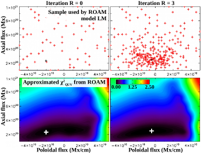
Figure 4.— Optimization results for sample $S^{\prime}_{7}$ (see Section 2.4) at the un-refined starting stage (left column) and at the refined final stage (right column) for model LM (see Table 1 for its parameter values). Top: Distribution of models in the parameter space (red “$+$” signs). Bottom: Corresponding approximated $\chi^{2}_{QUV}$ MSE (defined by Equation (10)). The black (top row) / white (bottom row) “$+$” sign indicates the position of the minimum found by ROAM.

Table 3Optimization results for all mean squared error tests
for ground-truth model LM

Minimized	$\Phi_{\mathrm{BF}}$	$\sigma_{\Phi}$	$\mathrm{F}_{\mathrm{BF}}$	$\sigma_{\mathrm{F}}$
MSE	(Mx)	(Mx)	(Mx cm${}^{-1}$)	(Mx cm${}^{-1}$)
$\chi^{2}_{QUV}$	$2.50\times 10^{20}$	$2.46\times 10^{17}$	$-4.00\times 10^{9}$	$2.18\times 10^{8}$
$\chi^{2}_{QU}$	$2.50\times 10^{20}$	$1.32\times 10^{17}$	$-3.93\times 10^{9}$	$8.85\times 10^{7}$
$\chi^{2}_{LAZV}$	$2.50\times 10^{20}$	$2.17\times 10^{17}$	$-4.00\times 10^{9}$	$1.85\times 10^{8}$
$\chi^{2}_{LAZ}$	$2.50\times 10^{20}$	$9.12\times 10^{16}$	$-3.98\times 10^{9}$	$4.75\times 10^{7}$

Note. — $\mu=(\Phi_{\mathrm{BF}},\mathrm{F}_{\mathrm{BF}})$ and $\sigma=(\sigma_{\Phi},\sigma_{\mathrm{F}})$ are the mean and standard deviation values computed from the seven best-fit vector parameters obtained after $R=3$ iterations of ROAM, as defined by Equations (2) and (3) in Section 2.4. The ground-truth model LM is defined by $(\Phi_{\mathrm{GT}},\mathrm{F}_{\mathrm{GT}})=(2.50\times 10^{20}\ \mathrm{Mx},\ -4.00\times 10^{9}\ \mathrm{Mx}\ \mathrm{cm}^{-1})$.

Table 4Optimization results vs. ground-truth parameters for $\chi^{2}_{QUV}$ minimization

Flux rope model	$\Phi_{\mathrm{GT}}$ (Mx)	$\Phi_{\mathrm{BF}}$ (Mx)	$\sigma_{\Phi}$ (Mx)	$\mathrm{F}_{\mathrm{GT}}$ (Mx cm${}^{-1}$)	$\mathrm{F}_{\mathrm{BF}}$ (Mx cm${}^{-1}$)	$\sigma_{\mathrm{F}}$ (Mx cm${}^{-1}$)	$R_{f}$
LL	$2.50\times 10^{20}$	$2.50\times 10^{20}$	$3.46\times 10^{16}$	$-1.00\times 10^{8}$	$-1.08\times 10^{8}$	$2.43\times 10^{7}$	5
LM	$2.50\times 10^{20}$	$2.50\times 10^{20}$	$2.46\times 10^{17}$	$-4.00\times 10^{9}$	$-4.00\times 10^{9}$	$2.18\times 10^{8}$	3
LH	$2.50\times 10^{20}$	$2.50\times 10^{20}$	$2.86\times 10^{17}$	$-1.00\times 10^{10}$	$-0.98\times 10^{10}$	$1.35\times 10^{8}$	3
ML	$5.00\times 10^{20}$	$5.00\times 10^{20}$	$3.46\times 10^{16}$	$-1.00\times 10^{8}$	$-1.02\times 10^{8}$	$6.79\times 10^{6}$	4
MM	$5.00\times 10^{20}$	$5.00\times 10^{20}$	$3.14\times 10^{16}$	$-4.00\times 10^{9}$	$-4.03\times 10^{9}$	$1.21\times 10^{7}$	3
MH	$5.00\times 10^{20}$	$5.00\times 10^{20}$	$7.48\times 10^{16}$	$-1.00\times 10^{10}$	$-1.00\times 10^{10}$	$1.48\times 10^{7}$	3
HL	$7.50\times 10^{20}$	$7.50\times 10^{20}$	$3.19\times 10^{17}$	$-1.00\times 10^{8}$	$-0.93\times 10^{8}$	$3.05\times 10^{7}$	3
HM	$7.50\times 10^{20}$	$7.49\times 10^{20}$	$6.36\times 10^{17}$	$-4.00\times 10^{9}$	$-3.95\times 10^{9}$	$1.26\times 10^{7}$	3
HH	$7.50\times 10^{20}$	$7.50\times 10^{20}$	$2.24\times 10^{17}$	$-1.00\times 10^{10}$	$-1.00\times 10^{10}$	$4.02\times 10^{7}$	3

Note. — $\mu=(\Phi_{\mathrm{BF}},\mathrm{F}_{\mathrm{BF}})$ and $\sigma=(\sigma_{\Phi},\sigma_{\mathrm{F}})$ are the mean and standard deviation values computed from the seven best-fit vector parameters obtained at the final iteration of ROAM, $R_{f}$, as defined by Equations (2) and (3) in Section 2.4.