Dynamic investment model of the life cycle of a company under the influence of factors in a competitive environment.

Abstract

Modelling all possible life cycles of a company in a highly competitive economic environment gives a significant advantage to the owner in his business investment activities. This article proposes and analyses a dynamic model of a company’s life cycle with known action costs and transition probabilities, that can be affected by an outside influence. For this task, the Markov model was utilized. The proposed model is illustrated on a task of determining an advertising policy for a car dealership, that would increase the stock equity of a company. The result demonstrates the usefulness of a model for use in determining future actions of a company. We also review multiple models of the influence of outside factors on a company’s total capitalization.

Keywords: Game theory; investment activities; strategy; optimization problem; Markov model; advertisement; deterministic model; stochastic model; decision tree; capitalization; decision-making

1 Introduction.

Dynamic decision-making game is the basis for modelling the influence of positive and negative factors on a company’s total capitalization. There are multiple possible models that can be applied to solve this problem. The Deterministic model takes into account the owner of a company, set of all possible states, discrete time variable, control function and some rational function. The Stochastic model adds to this a probability of transition from one state to another. We demonstrate stochastic model on an example by building a decision tree and finding an optimal strategy for the release of a new product on the national market. We also look at the probabilistic - deterministic model and demonstrate it on a simple example.

Markov models are very effective in many different fields which rely on sequential decision making. At each step, the decision maker considers the current state and makes a decision with a goal to maximize a company’s total capitalization, which leads a company to the next state. Action costs and transition probabilities are mainly responsible for how the system behaves.

As an example of an application of this model, we use a car dealership’s marketing campaign. We apply our model to help the owner chose an optimal advertising policy for every city. This model uses transitional probabilities and profits as input data for Howard’s improvement algorithm. This algorithm is chosen because of its simplicity and effectiveness in deciding which policy is optimal.

Many ideas that are used in this work are taken from [1]-[60]

2 Literature Review.

There are some previously conducted studies related to the use of the Markov model which are summarized below.
Merve Merakli and Simge Kucukyavuz used Markov Decision Processes to solve an inventory management problem for humanitarian relief operations during a slow-onset disaster.
C. Drent, S. Kapodistria, and J. A. C. Resing formulated condition based maintenance policies under imperfect maintenance at scheduled and unscheduled opportunities as a semi-Markov decision process, and used it to find an optimal policy.
Yu-Yang Zhou and Guang Cheng used Multi-Objective Markov Decision Processes in their novel shuffling method against DDoS attacks.
Sebastian Junges, Erika Abraham, Christian Hensel, Nils Jansen, Joost-Pieter Katoen, Tim Quatmann, Matthias Volk developed multiple analysis algorithms for parametric Markov chains and Markov decision processes.
Thiago Freitas dos Santos, Paulo E. Santos, Leonardo A. Ferreira, Reinaldo A. C. Bianchi, Pedro Cabalar used Markov Decision Process to solve spatial puzzles.
Takashi Tanaka, Ehsan Nekouei, Ali Reza Pedram, Karl Henrik Johansson showed that mean-field approximation of a dynamic traffic routing game over an urban road network leads to the linearly solvable Markov decision process.

3 Deterministic model of the influence of positive and negative factors on activities of a company’s investment activities.

3.1 Informal formalization of the task of constructing and analysing a deterministic model of the influence of positive and negative factors on investment activities of a company.

Let be

$$\Gamma=\Gamma\langle N,X=\{X_{i}^{j}\}_{0_{1}}^{n^{m}},t=\{0,1,...,n\},U=\{u_{i}^{j}\}_{1_{1}}^{n^{m}},R=\{r_{i}^{j}\}_{1_{1}}^{b^{m}}\rangle$$

– dynamic decision-making game by an owner of a business with full information. Here N - the owner of a company, making the decisions. X - set of all states of a company. t - discrete value, denoting time. U - control function, determining the transition from state $X_{i}$ to state $X_{i+1},U_{i+1}:X_{i}\rightarrow X_{i+1}$. R - rational function is given on the set of all controls. The sum value of this function on controls is called a total win. Depending on what decision is made(control at the current stage) development of a company occurs according to one of the schemes, which implies an action of the collection, of positive factors $\alpha_{i}$, and negative factors $\beta_{i}$, while a company is in state $\Omega$.

Among controls, emerging from the point X we are required to choose a control with maximum sum total capitalization.

3.2 Formalization of the task of constructing and analysing a deterministic model of the influence of factors on a company’s investment activities.

Initially, the owner starts in a state $X_{0}$ and makes a management decision $u_{1}^{j}\in U_{1}$, i.e chooses one of the possible controls in this state. After that company transitions to state $X_{1}$. After that, internal and external factors with positive and negative influence start to affect company’s investment activities. Because of this growth or decline of capitalization of a company is possible.

For example, the purchase of new equipment causes an increase in production volume. That, in turn, can cause multiple outcomes. The best one being – an increase in profits. With stable demand, purchasing new equipment with higher performance is inadvisable.

During the second step, the owner again makes a management decision $u_{2}^{j}\in U_{2}$, by choosing from a set of available controls. A company transitions to the next state - $X_{2}$.After that, internal and external factors with positive and negative influence start to affect a company, and so on.

On step n the owner chooses $u_{n}^{j}\in U_{n}$ one of the possible controls during this stage. After that a company transitions to the final step. During a transition from $X_{i}$ to $X_{i+1}$, a company’s capitalization rises or declines. In final state $X_{n}$ capitalization of a company is defined as total capitalization during a previous step.

Thus, the problem will be solved, then a company’s capitalization is be defined for each point and a maximum will be found.

4 Stochastic model of the influence of negative and positive factors on a company’s investment activities.

4.1 Informal formulation of the problem of building and analysing a stochastic model of the influence of negative and positive factors on a company’s investment activities.

Let be

$$\Gamma=\Gamma\langle N,X=\{X_{i}^{j}\}_{0_{1}}^{n^{m}},t=\{0,1,...,n\},U=\{u_{i}^{j}\}_{1_{1}}^{n^{m}},P=\{p_{i}^{j}\}_{1_{1}}^{n^{m}},R=\{r_{i}^{j}\}_{1_{1}}^{b^{m}}\rangle$$

– a dynamic decision-making game for the owner of a company, where N – is the owner, who makes decisions. X – a set of all possible states of a company. t – a discrete value, denoting time, which determines the step number. U – a control function, which defines a transition from state $X_{i}$ to state $X_{i+1}$. R – a rational function, which is defined on a set of all controls. A sum of function R is called a sum total of company’s capitalization. $p_{i}^{j}$ – a probability of transition from state $X_{i}$ to state $X_{i+1}$.

Among controls, emerging from the point X we are required to choose a control with maximum sum total capitalization.

4.2 Formulation of the problem of building and analysing the deterministic model of influences by factors on a company’s investment activities.

The model is described as follows. On initial stage entrepreneur - is an owner of a company, in state $X_{0}$ makes a decision. Then, a company’s investment activities are affected by both external and internal factors that have either positive or negative effects. Entrepreneur possesses information, that events of the second stage from $X_{2}$ may occur with a certain probability P. The sum of even probabilities from each stage = 1. The entrepreneur knows possible outcome options, their probabilities and will there be a rise or fall of a company’s capitalization, depending on his decision, and by what amount. The uncertainty lies in the fact that the entrepreneur cannot determine what influence external factors will have on the choice of a particular decision.

Example.

A company is deciding on the introduction of a new product on the national market. Uncertainty lies in, how will the market react to a new product. Test launch of a new product in the regional market is being considered. This way, the initial decision, which a company needs to make is – should product’s marketing start on a regional level. A company states, that launch on a regional market requires an initial investment of four million dollars, and launch on the national market required an investment of eighty million dollars. If trial sales at the regional level are not conducted, the decision to enter the national market can be made immediately.

A company considers sales number as successful, mediocre or negative, depending on volume sold. For the regional level, this equates to sale volumes of 500, 200 and 50 thousand units, and for the national 10000, 5000 and 1000 thousand units respectively. Based on the data, from the regional testing of similar products, a company assesses the probabilities of these three outcomes as 0.2, 0.7 and 0.1. Besides this, after researching the data about the relation of regional sales results with subsequent sales on the national market, a company has managed to estimate the following conditional probabilities.

		Conditional probabilities of sales in the nationwide market
			Successful	Mediocre	Negative
Probability of sales in the regional market	0.2	Successful	0.75	0.2	0.05
	0.7	Mediocre	0.35	0.5	0.15
	0.1	Negative	0.05	0.3	0.65

Besides that, it is known, that each sale brings a profit of 25 dollars on both local and national markets.

The problem is to make a valid strategy for entering (or not entering) the market with a new product.

Solution: We consider three main components for situations of this type. After that, we will build a decision tree for this problem.

Let us calculate decision tree’s characteristics.

Probabilities of sales levels in the nationwide market without initial regional market launch:

• Successful: $(0.75*0.2)+(0.35*0.7)+(0.05*0.1)=0.4$

• Mediocre: $(0.2*0.2)+(0.5*0.7)+(0.3*0.1)=0.42$

• Negative: $(0.05*0.2)+(0.15*0.7)+(0.65*0.1)=0.18$

Revenue from a national market launch:

• Successful: $10000*25=250000$

• Mediocre: $5000*25=125000$

• Negative: $1000*25=25000$

Profits from a national market launch without initial regional market launch:

• Successful: $250000-80000=170000$

• Mediocre: $125000-80000=45000$

• Negative: $25000-80000=-55000$

Results on a national market without initial regional market launch:
$0.4*250000+0.42*125000+0.18*25000-80000=77000$

Revenue from a regional market launch:

• Successful: $500*25=12500$

• Mediocre: $200*25=5000$

• Negative: $50*25=1250$

Profits from a regional market launch:

• Successful: $12500-4000=8500$

• Mediocre: $5000-4000=1000$

• Negative: $1250-4000=-2750$

Profits from a national market launch with initial successful regional market launch:

• Successful: $250000-80000+8500=178500$

• Mediocre: $125000-80000+8500=53500$

• Negative: $25000-80000+8500=-46500$

Probabilities of sales levels in nationwide market with initial successful regional market launch:

• Successful: $0.2*0.75=0.15$

• Mediocre: $0.2*0.2=0.04$

• Negative: $0.2*0.05=0.01$

Result on a national market with initial successful regional market launch:
$250000*0.75+125000*0.2+25000*0.05-80000+12500-4000=142250$

Profits from a national market launch with initial mediocre regional market launch:

• Successful: $250000-80000+1000=171000$

• Mediocre: $125000-80000+1000=46000$

• Negative: $25000-80000+1000=-54000$

Probabilities of sales levels in nationwide market with initial mediocre regional market launch:

• Successful: $0.7*0.35=0.245$

• Mediocre: $0.7*0.5=0.35$

• Negative: $0.7*0.15=0.105$

Result on a national market with initial mediocre regional market launch:
$250000*0.35+125000*0.5+25000*0.15-80000+5000-4000=74750$

Profits from a national market launch with initial negative regional market launch:

• Successful: $250000-80000-2750=167250$

• Mediocre: $125000-80000-2750=42250$

• Negative: $25000-80000-2750=-57750$

Probabilities of sales levels in nationwide market with initial negative regional market launch:

• Successful: $0.1*0.05=0.005$

• Mediocre: $0.1*0.3=0.03$

• Negative: $0.1*0.65=0.065$

Result on a national market with initial negative regional market launch:
$250000*0.05+125000*0.3+25000*0.65-80000+1250-4000=-12900$

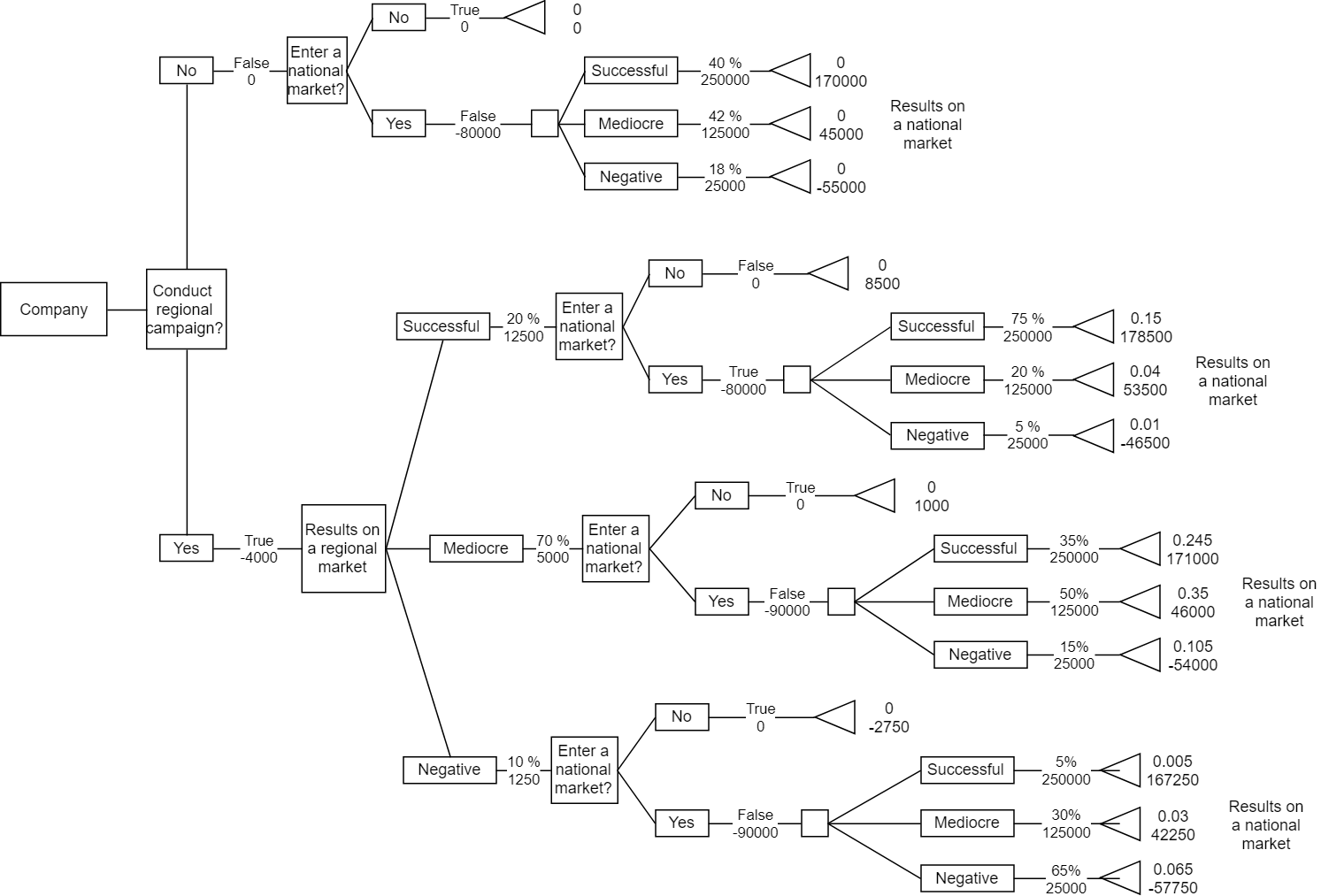
Figure 1: Product launch decision tree.

Thus, by analysing the decision tree, we can formulate an optimal strategy for a company, namely: it is necessary to make a preliminary sales in the regional market and to expand sales at the national level, only if results during regional trials prove to be successful.

5 Probabilistic - deterministic model of influences by negative and positive factors on a company’s investment activities.

5.1 Informal statement of the problem of constructing and analysing a probabilistic-deterministic model of influences by negative and positive factors on a company’s investment activities.

Let be

$$\Gamma=\Gamma\langle N,X=\{X_{i}^{j}\}_{1}^{n},t=\{0,1,...,n\},U=\{u_{t}\}_{1}^{n},R=\{r_{k}\}_{1}^{c}\rangle$$

- a dynamic game of decision-making by the owner of a company with complete information, where N is the owner of a company making decisions. X is the set of all company’s states. t - discrete value denoting time. U - control function that determines the transition from state X to state $X_{i+1},U_{i+1}:X_{i}\rightarrow X_{i+1}$. R - a rational function defined on the set of all controls.

5.2 Formulation of the problem of building and analysing a probabilistic - deterministic model of influences by negative and positive factors on a company’s investment activities.

Now suppose that the choice of control at a point X does not determine a state, but only a probability distribution for this state.

Let $X_{t}$ and $U_{t}$ be arbitrary finite sets. Each u from $U_{t}$ is mapped to probability distribution p on $X_{t}$. The function p, that defines the law of transition from $U_{t}$ to $X_{t}$, will be called the transition function. It is assumed that the point $X_{0}$ from the set from which the game begins is also random, and its probability distribution $\mu$ (initial distribution) is given.

The transition from x$\in X_{t-1}$ to $U_{t}$ is determined by the entrepreneur. In this case, we choose u not from all of $U_{t}$, but from its subset $U\left(x\right)$, that is dependant on the state x. The elements of a set $U\left(x\right)$ will be called controls at a point x. Sets $U\left(x\right)$ are defined and not empty for all non-final states. It is assumed that $U\left(x\right)$ do not intersect in pairs and their sum of all $x\in X_{t-1}$ is equal to $U_{t}$. In other words, each control u can be used in one and only one state. We denote this state as $j\left(u\right)$, so the record $x=j\left(u\right)$ is equivalent to the record $u\in U\left(x\right)$.

On the set of all controls, the current growth or decline of a company’s capitalization $r\left(u\right)$ is given, and on the set of final states - the final growth or decline of a company’s capitalization $r\left(x\right)$ is given.

The model is described as follows. At the initial moment of time, the entrepreneur - the owner of a company - makes a decision, chooses a control - a set of transition probabilities at the current stage. Then the second participant - nature chooses the next state. For the transition from state 0 to state 1, the owner receives a certain capitalization of a company.

The purpose of the model is to obtain the maximum capitalization of a company.

Example.

The column $U_{1}$ shows three probability distributions on the set $X_{1}$, corresponding to the three controls from $X_{0}$. The column $U_{2}$ indicates five probability distributions on the set $X_{2}$, that correspond to the controls from the state $X_{1}$. The problem will be solved if we find the control with the maximum increase in the capitalization of a company.

In state 3 expected value equals:

$0+\frac{1}{2}*1+\frac{1}{2}*2=\frac{3}{2}$

when choosing the first control and equals

$1+\frac{1}{4}*1+\frac{3}{4}*2=\frac{11}{4}$

when choosing the second. The estimate of state 3 is equal to the maximum of these two numbers, i.e. $\frac{11}{4}$ and it is clear that under state 3 one should prefer the second control.

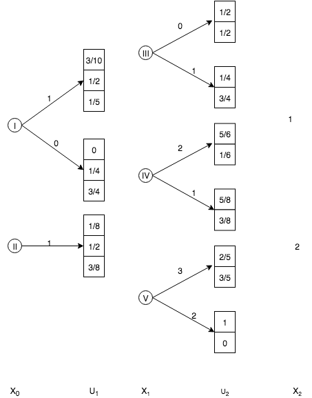
Figure 2: Model.

Similarly,

$v\left(IV\right)=max\left(2+\frac{5}{6}*1+\frac{1}{6}*2;1+\frac{5}{8}*1+\frac{3}{8}*2\right)=\frac{19}{6},$

in state 4, the first control is preferable.

$v\left(V\right)=max\left(3+\frac{2}{5}*1+\frac{3}{5}*2;2+1*1+0*2\right)=\frac{23}{5},$

In state 5, the first control is more profitable. Next, choosing in state 1 the first control, and then, acting in an optimal way, we obtain an estimate,

$1+\frac{3}{10}*\frac{11}{4}+\frac{1}{2}*\frac{19}{6}+\frac{1}{5}*\frac{23}{5}=\frac{2597}{600}$

and choosing the second state, we obtain an estimate

$0+0*\frac{11}{4}+\frac{1}{4}*\frac{19}{6}+\frac{3}{8}*\frac{23}{5}=\frac{151}{60}$

6 Stochastic decision-making investment model of company’s life cycle.

6.1 Informal statement of the problem of constructing and analysing a stochastic decision-making investment model of company’s life cycle.

A model $\Gamma=\langle I=\{1,2,...,n\}=\{i\}_{1}^{k},K_{i}=\{1,2,...,k_{i}\},S_{i}=\{s_{i}\}_{1}^{n},R_{i}\rangle$ is considered, in which the decision-making process is represented by a finite number of states i, i = 1,2, …, n.

Let each state $i\in S=\{1,...,N\}$ correspond to a finite set of solutions (or alternatives) $K_{i}$, the elements of which we denote by numbers 1,…,$k_{i}$. The space of strategies K is the direct product of sets of solutions K = $K_{1}\times K_{2}\times...\times K_{n}$.

Exists a matrix $P=(p_{i}j)$ of transition probabilities between states. The reward structure is represented in the form of a matrix $R\left(q\right)=\left(r_{ij}\left(q\right)\right)$, the elements of which are the income values. The matrix of transition probabilities P and the income matrix $R\left(q\right)$ depend on the decision policies k by the decision maker.

Depending on what decision is made (control at the current stage), the development of a company proceeds according to one or another scheme, which implies an influence by a combination of positive factors $\alpha_{i}$ and negative factors $\beta_{i}$ on the state of a company $\Omega$.

There is a finite set of company’s states i, which is estimated by the value of a company’s capitalization per unit of time t. Depending on the decision taken, a company goes into one of the possible states i. In each state i, the set of rational strategies k depends on this state.

The goal of the task is to find the optimal strategy that maximizes the expected capitalization of a company from a process that has a finite number of stages.

6.2 Formulation of the problem of constructing and analysing a stochastic decision making investment model of company’s life cycle.

Let the process of transition from state to state occur, not deterministically, but stochastically and controlled by the transition matrix $P=\left(p_{ij}\right)$, where $p_{ij}$ is the probability that the system at the time t+1 is in the state j, if it is known, that at the time t it was in the state i.

Consider the case, when the matrix does not depend on time, and decisions are made at each step. Suppose that at each step one of the sets of such matrices can be chosen as a transition matrix, and we denote the matrix, corresponding to policy q, as $P\left(q\right)=\left(p_{ij}\left(q\right)\right)$.

Suppose further that not only the state at each step changes but also the capitalization of a company, which is a function of the initial and final states and the solution.

Let $R\left(q\right)=\left(r_{ij}\left(q\right)\right)$ denote the corresponding matrix of a company’s capitalization.

Note that this model is not perfect since the same factor can be both positive and negative. Examples are a change in technology, personnel, investment, etc. In order to get the closer details of specific tasks, the stochastic model will be discussed below using a specific example.

7 Classification of a company’s investment activities in the Markov model of control of its activities.

We introduce a classification based on a company’s key performance indicators (for example, sales of goods and/or services, productivity, profits, customer satisfaction, etc.); in this case, we will consider the growth of stock prices, x(t). We introduce the following indicators:

• growth rate, $V\left(t\right)=\frac{x\left(t\right)}{t}$;

• growth acceleration, $a\left(t\right)=\frac{V\left(t\right)}{t}$.

Thus, if the growth rate is zero, a company is in a stable state (there is no rise and fall in stock prices); if the growth rate is greater than zero, then a company is in a state of growth, because its shares are growing; if it is less than zero, then a company is in decline (stock quote falls). Acceleration largely characterizes stable conditions not only of a company but also of the stock market as a whole, since It shows spasmodic processes of rising or falling stock prices.

7.1 Car dealership

Suppose that a car dealership operates in five cities. In any of these cities we can invest in an advertisement in the following areas:

• 1 - advertisement on the radio;

• 2 - placing ads on the website;

• 3 - placement of advertisements in the printed publication ”Car Bulletin”;

• 4 - TV adverts;

• 5 - active search for customers.

In each city for all of these fixed policies, the probabilities are set that the next customer will acquire a car in one of the five cities and the corresponding income in monetary terms associated with each sale. Since each policy has a different set of clients, transition probabilities and revenues depend on the policies. Income, in this case, is expressed as a fall or an increase in the capitalization of a company.

If we assign some hypothetical numbers to them, then these tasks can be written in a table.

State (city)	Policy	Transition probability					Profit
		j = 1	2	3	4	5	i = 1	2	3	4	5
1	1	0.1	0.2	0.4	0.1	0.2	-300	-200	-190	280	-120
	2	0.2	0.2	0.1	0.5	0	940	-270	-600	80	620
	3	0.7	0.1	0	0	0.2	-60	100	520	-760	230
	4	0.2	0.1	0.2	0.3	0.2	20	110	0	390	510
	5	0.2	0.1	0.1	0.4	0.2	620	0	-640	250	630
2	1	0.1	0.2	0.2	0.2	0.3	0	330	680	-240	390
	2	0	0.1	0.1	0.3	0.5	270	640	320	0	-480
	3	0.1	0.5	0.2	0	0.2	460	-480	0	180	570
	4	0.3	0.2	0.3	0	0.2	-320	840	750	730	690
	5	0.4	0.3	0.1	0.2	0	560	510	-90	120	0
3	1	0.3	0	0.4	0.2	0.1	170	120	180	-300	280
	2	0.5	0.2	0	0.2	0.1	220	-60	150	0	660
	3	0.1	0.2	0.5	0.1	0.1	110	20	100	-160	90
	4	0	0.1	0.4	0.3	0.1	170	170	0	300	-880
	5	0.4	0	0.1	0.4	0.1	-660	480	810	830	240
4	1	0.2	0.2	0.1	0.1	0.4	-100	0	800	150	560
	2	0	0.1	0.2	0.6	0.1	620	560	470	-620	400
	3	0.5	0.1	0.1	0.2	0.1	170	250	0	-280	0
	4	0.3	0.1	0.1	0.5	0	500	630	920	430	90
	5	0.3	0.3	0.1	0.1	0.1	80	510	-110	110	300
5	1	0.1	0.3	0.1	0.4	0.1	710	-160	50	280	690
	2	0.2	0.2	0	0.2	0.4	920	100	600	270	180
	3	0	0.1	0.1	0.7	0.1	0	740	710	-60	160
	4	0.1	0.1	0.1	0.3	0.4	500	980	900	220	580
	5	0.4	0.1	0.3	0	0.2	520	400	960	60	690

Lets us explain the table using the last row as an example. It shows that investment in the first policy (advertising on the radio) in the fifth city, will lead to a probability of 0.1 that there will be a sale in city 1, and there will be an increase in the capitalization of a company by 710 units. With a probability of 0.3, there will be a sale in city 2 with a loss of 160 units, and a probability of 0.1 that there will be a sale in city 3, with an income of 50 units, a probability of 0.4 that the sale will occur in city 4, with an income of 280 units and a probability of 0.1 that there will be a sale in city 5, and the capitalization of a company will increase by 690 units.

There are five states in this problem, i.e. N = 5, and five policies in states 1, 2, 3, 4, 5, i.e. $n_{1}=5,n_{2}=5,n_{3}=5,n_{4}=5,n_{5}=5$. This means that there are 5 * 5 * 5 * 5 * 5 = 3125 possible policies


Solution:

As the initial approximation, the policy vector D will be chosen as,

$D=\begin{bmatrix}1\\ 1\\ 1\\ 1\\ 1\end{bmatrix}$

which means that we work in all cities. This is a policy that maximizes the expected value of a company’s capitalization growth. For this policy, we have a matrix of transition probabilities P

$P=\begin{bmatrix}0.1&0.2&0.4&0.1&0.2\\ 0.1&0.2&0.2&0.2&0.3\\ 0.3&0&0.4&0.2&0.1\\ 0.2&0.2&0.1&0.1&0.4\\ 0.1&0.3&0.1&0.4&0.1\end{bmatrix}$

The sum $\sum_{j=1}^{N}p_{ij}r_{ij}$ will be denoted as $q_{i}$, since the expected capitalization of a company depends only on i. The equation for determining the values of $v_{i}$, assuming a value of $v_{3}$ is zero, is written as

$\begin{array}[]{lcl}g+v_{1}=-142+0.1v_{1}+0.2v_{2}+0.4v_{3}+0.1v_{4}\\ g+v_{2}=271+0.1v_{1}+0.2v_{2}+0.2v_{3}+0.2v_{4}\\ g+v_{3}=91+0.3v_{1}+0v_{2}+0.4v_{3}+0.2v_{4}\\ g+v_{4}=299+0.2v_{1}+0.2v_{2}+0.1v_{3}+0.1v_{4}\\ g=209+0.1v_{1}+0.3v_{2}+0.1v_{3}+0.4v_{4}\end{array}$

and have a solution

$\begin{array}[]{lcl}g=150.78\\ v_{1}=-458.25\\ v_{2}=21.58\\ v_{3}=-317.98\\ v_{4}=32.32\\ v_{5}=0\\ \end{array}$

Using the policy of ”advertising on the radio” dealership will have an average of 150.78 units gained per transaction.

Referring to the policy improvement procedure, let us calculate the values of $q_{i}^{k}+\sum_{j=1}^{N}p_{ij}^{k}v_{j}$ for all i and k.

i	k	$q_{i}^{k}+\sum_{j=1}^{N}p_{ij}^{k}v_{j}$
1	1	-307.469
	2	11.028
	3	-304.617
	4	90.608
	5	177.638	+
2	1	172.359
	2	-163.944
	3	-178.631
	4	206.447	+
	5	189.84
3	1	-167.203
	2	-54.345
	3	-139.267
	4	-96.338
	5	-29.17	+
4	1	-23.013
	2	-562.917
	3	-408.7958
	4	74.347	+
	5	-225.7162
5	1	150.779
	2	249.14
	3	111.984
	4	470.231	+
	5	397.464

We see that for i = 1 the value in the right column is maximum for k = 5. Similarly for i = 3. For i = 2, i = 4 and i = 5 the value is maximum for k = 4. In other words, the new policy will be determined by vector D.

$D=\begin{bmatrix}5\\ 4\\ 5\\ 4\\ 4\end{bmatrix}$

This means that in the first, third and fifth cities it is most advantageous to use the 5th policy and for the second and fourth cities to use the fourth.

Now we have

$P=\begin{bmatrix}0.2&0.1&0.1&0.4&0.2\\ 0.3&0.2&0.3&0&0.2\\ 0.4&0&0.1&0.4&0.1\\ 0.3&0.1&0.1&0.5&0\\ 0.1&0.1&0.1&0.3&0.4\end{bmatrix}\begin{bmatrix}q_{i}\end{bmatrix}=\begin{bmatrix}209\\ 330\\ 119\\ 536\\ 674\end{bmatrix}$

Let us solve the equations

$\begin{array}[]{lcl}g+v_{1}=209+0.2v_{1}+0.1v_{2}+0.1v_{3}+0.4v_{4}+0.2v_{5}\\ g+v_{2}=330+0.3v_{1}+0.2v_{2}+0.3v_{3}+0v_{4}+0.2v_{5}\\ g+v_{3}=119+0.4v_{1}+0v_{2}+0.1v_{3}+0.4v_{4}+0.1v_{5}\\ g+v_{4}=536+0.3v_{1}+0.1v_{2}+0.1v_{3}+0.5v_{4}+0v_{5}\\ g+v_{5}=674+0.1v_{1}+0.1v_{2}+0.1v_{3}+0.3v_{4}+0.4v_{5}\end{array}$

Assuming again that $v_{5}$ is zero, we get

$\begin{array}[]{lcl}g=400.633\\ v_{1}=-551.143\\ v_{2}=-555.888\\ v_{3}=-695.783\\ v_{4}=-310.286\\ v_{5}=0\\ \end{array}$

Note that g has increased from 150.79 to 400.633, so the agency earns an average of 400.633 units per transaction. Using the policy improvement algorithm for these values, we calculate the values $q_{i}^{k}+\sum_{j=1}^{N}p_{ij}^{k}v_{j}$ for all i and k.

i	k	temp
1	1	-617.6337
	2	-332.1275
	3	-427.3889
	4	-164.0598
	5	-73.5101	+
2	1	-96.5057
	2	-362.2529
	3	-552.2149
	4	-50.2554	+
	5	-126.8591
3	1	-414.7133
	2	-284.8063
	3	-487.212
	4	-407.9878
	5	-241.1499	+
4	1	183.1
	2	-224.046
	3	-198.301
	4	369.045	+
	5	47.433
5	1	-206.5734
	2	46.5366
	3	-223.3673
	4	262.6328	+
	5	189.2191

The new policy is thus determined by the vector D.

$D=\begin{bmatrix}5\\ 4\\ 5\\ 4\\ 4\end{bmatrix}$

Which coincides with the vector of the previous policy, the process has converged, and the value reached its maximum equal to 400.633. The agency must actively search for clients in the first and third city, but use TV adverts in the rest. The application of this policy will give, on average, per transaction, an income of 419.2 units.

References

- [1] I.V.Zaitseva, E.N.Kriulina, O.A.Malafeyev Model of dynamic in interregional migrational flows of labour resources. Nikon readings. 2018. No. 23. S. 263-265. 1972. 4. S. 41-46.
- [2] Zaitseva I., Ermakova A., Shlaev D., Malafeyev O., Strekopytov S. Game-Theoretical model OF labour force training. Journal of Theoretical and Applied Information Technology. 2018. T. 96. No. 4. S. 978-983.
- [3] O.A. Malafeyev, Redinskikh N.D. Model of planning of basic geopolitical operations with the possible support of the subsidiary activities. Control Processes and Stability. 2018. T. 5. No 1. S. 479-481.
- [4] O.A. Malafeyev, Sicheva S.A. Mathematical methods and models in speed construction. Saint-Petersburg 2017.
- [5] Malafeyev O.A., Rylov D.S., Zaitseva I.V., Novozhilova L.M. Differential game model of dispersed material drying. No. arXiv:1705.11129 19.05.2017
- [6] Kiryanen A.I., Malafeyev O.A., Redinskikh N.D. Stability in the process with lag of interaction between mining and processing industries. No arXiv:1706.06010 06.06.2017
- [7] Pichugin Yu.A., Malafeyev O.A., Rylov D.S. A statistical method for corrupt agents detection. No. arXiv:1707.04461v1 14.07.2017
- [8] Malafeyev O.A., Rylov D.S., Zaitseva I.V., Ermakova A., Shlaev D. Multistage voting model with alternative elimination. No arXiv:1707.06189v1 19.07.2017
- [9] Malafeyev O.A., Farvazov K., Zenovich O. Geopolitical model of investment project implementation. No arXiv:1707.06829v1 21.07.2017
- [10] Malafeyev O.A., Awasthi A., Kambekar K.S. Random walks and market efficiency in chinese and indian equity markets. No. arXiv:1707.06189v1 19.07.2017
- [11] Kolesin I.D., Malafeyev O.A., Zaitseva I.V., Ermakova A.N., Shlaev D.V. Modeling of the labour force redistribution in investment projects with account of their delay. No. arXiv:1707.06189v1 19.07.2017
- [12] Malafeyev O.A., Redinsky N. D., Zaitseva I.V. Problem of distribution of income in the company. No. arXiv:1709.06380v1 19.09.2017
- [13] Malafeyev O.A., Awasthi A. Dynamic optimization of a portfolio. No. arXiv:1712.00585v1 02.12.2017
- [14] Zaitseva I., Ermakova A., Shlaev D., Malafeyev O., Kolesin I. Modeling of the labour force redistribution in investment projects with account of their delay. In: IEEE International Conference on Power, Control, Signals and Instrumentation Engineering, ICPCSI 2017 2017. S. 68-70.
- [15] Malafeyev O.A., Redinskikh N.D. Quality estimation of the geopolitical actor development strategy. In: 2017 Constructive nonsmooth analysis and related topics (dedicated to the memory of V.F. Demyanov) (CNSA) 2017. S. 7973986.
- [16] Malafeyev O., Rylow D., Novozhilova L., Zaitseva I., Popova M., Zelenkovskii S. Game-theoretic model of dispersed material drying process. In: AIP Conference Proceedings ”International Conference on Functional Materials, Characterization, Solid State Physics, Power, Thermal and Combustion Energy, FCSPTC 2017” 2017. S. 020063.
- [17] Malafeyev O.A., Rylow D., Kolpak E.P., Nemnyugin S.A., Awasthi A. Corruption dynamics model. In: AIP Conference Proceedings ”International Conference of Numerical Analysis and Applied Mathematics, ICNAAM 2016” 2017. S. 170013.
- [18] Kolesin I., Malafeyev O., Andreeva M., Ivanukovich G. Corruption: taking into account the psychological mimicry of officials. In: AIP Conference Proceedings ”International Conference of Numerical Analysis and Applied Mathematics, ICNAAM 2016” 2017. S. 170014.
- [19] Malafeyev O., Saifullina D., Ivaniukovich G., Marakhov V., Zaytseva I. The model of multi-agent interaction in a transportation problem with a corruption component. In: AIP Conference Proceedings ”International Conference of Numerical Analysis and Applied Mathematics, ICNAAM 2016” 2017. S. 170015.
- [20] Malafeyev O.A, Redinskikh N.D. Quality assessment of the development strategy of the geopolitical actor. In: Constructive Nonsmooth Analysis and Related Topics 2017. S. 237-420.
- [21] Kolokoltsov V.N., Malafeyev O.A. Mean-field-game model of corruption. Dynamic Games and Applications. 2017. T. 7. No 1. Pp. 34-47.
- [22] Malafeyev O., Saifullina D., Ivaniukovich G., Marakhov V., Zaytseva I. Dynamic model of corruption and legal investments. Control Processes and Stability. 2017. T. 4. No 1. S. 647-651.
- [23] Kirjanen A.I., Malafeyev O.A., Redinskikh N.D. Developing industries in cooperative interaction: equilibrium and stability in processes with lag. Statistics, Optimization and Information Computing. 2017. T. 5. No 4. Pp. 341-347.
- [24] Malafeyev O., Saifullina D., Ivaniukovich G., Marakhov V., Zaytseva I. Study of corruption processes and systems by mathematical methods. Innovative technologies in engineering, education and economics. 2017. Vol. 3. No. 1-1 (3). Pp. 7-13.
- [25] Malafeyev O.A., Marakhov V.G. Evolutionary mechanism of actions of sources and moving forces of civil society in the field of financial and economic components of the XXI century. In the book: Civil Society in Russia and its prospects in the XXI century St. Petersburg, 2017. P. 98-116.
- [26] Malafeyev O.A., Zaitseva I.V., Popova M.V. Mathematical methods used to solve the state security problem. In the collection: Security service in russia: experience, problems, prospects. ensuring the complex safety of the population life the materials of the IXth All-Russian Scientific Practical Conference. St. Petersburg University of the State Fire Service EMERCOM of Russia. 2017. pp. 330-334.
- [27] Zaitseva I.V., Malafeyev O.A., Strekopytov S.A. Economic and mathematical models of economic system management. In the collection: Management of socio-economic systems: methods, models, technologies Collection of scientific papers on the materials of the II International Scientific and Practical Conference. 2017. pp. 21-27.
- [28] Malafeyev O.A., Redinskikh N.D., Rumyantsev N. Multi-agent interaction in social trading network. Article in the open archive No. 1609.06244v1 09/16/2016
- [29] Kolokoltsov V.N., Malafeyev O.A. Corruption and botnet defense: a mean field game approach. Article in the open archive No. 1607.07350 25.07.2016
- [30] Malafeyev O.A., Redinskikh N.D. Stochastic analysis of the dynamics of corrupt hybrid networks. In the collection: 2016 International Conference ”Stability and Oscillations of Nonlinear Control Systems” (Pyatnitskiy’s Conference 2016) 2016. pp. 7541208.
- [31] Pichugin Y.A., Malafeyev O.A. Statistical estimation of corruption indicators in the firm. Applied Mathematical Sciences. 2016. T. 10. No 41-44. pp. 2065-2073.
- [32] Pichugin Y., Alferov G., Malafeyev O. Parameters estimation in mechanism design. Contemporary Engineering Sciences. 2016. T. 9. No 1-4. pp. 175-185.
- [33] Awasthi A., Malafeyev O.A. Is the indian stock market efficient - a comprehensive study of Bombay stock exchange indices. Article in the open archive number No. 1510.03704 10.10.2015
- [34] Awasthi A., Malafeyev O.A. A dynamic model of functioning of a bank. Article in the open archive number No. 1511.01529 03.11.2015
- [35] Kolokoltsov V.N., Malafeyev O.A. Mean field game model of corruption. Article in the open archive number No. 1507.03240 12.07.2015
- [36] Malafeyev O.A., Nemnyugin S.A., Ivaniukovich G.A. Stochastic models of social-economic dynamics. In the collection: 2015 International Conference ”Stability and Control Processes” in Memory of V.I. Zubov (SCP) 2015. pp. 483-485.
- [37] Neverova E.G., Malafeyev O.A., Alferov G.V., Smirnova T.E. Model of interaction between anticorruption authorities and corruption groups. In the collection: 2015 International Conference ”Stability and Control Processes” in Memory of V.I. Zubov (SCP) 2015. pp. 488-490.
- [38] Alferov G.V., Malafeyev O.A., Maltseva A.S. Programming the robot in tasks of inspection and interception. In the collection: 2015 International Conference on Mechanics - Seventh Polyakhov’s Reading 2015. pp. 7106713.
- [39] Malafeyev O., Alferov G., Andreyeva M. Group strategy of robots in game-theoretic model of interception with incomplete information. In the collection: 2015 International Conference on Mechanics - Seventh Polyakhov’s Reading 2015. pp. 7106751.
- [40] Alferov G.V., Malafeyev O.A., Maltseva A.S. Game-theoretic model of inspection by anti-corruption group. In the collection: AIP Conference Proceedings 2015. pp. 450009.
- [41] Malafeyev O.A., Nemnyugin S.A., Alferov G.V. Charged particles beam focusing with uncontrollable changing parameters. In the collection: 2nd International Conference on Emission Electronics (ICEE) Selected papers. Proceedings Edited by: N. V. Egorov, D. A. Ovsyannikov, E. I. Veremey. 2014. pp. 25-27.
- [42] Malafeyev O.A., Redinskikh N.D., Alferov G.V. Electric circuits analogies in economics modeling: corruption networks. In the collection: 2nd International Conference on Emission Electronics (ICEE) Selected papers. Proceedings Edited by: N. V. Egorov, D. A. Ovsyannikov, E. I. Veremey. 2014. pp. 28-32.
- [43] Malafeyev O.A., Neverova E.G., Nemnyugin S.A., Alferov G.V. Multi-criteria model of laser radiation control. In the collection: 2nd International Conference on Emission Electronics (ICEE) Selected papers. Proceedings Edited by: N. V. Egorov, D. A. Ovsyannikov, E. I. Veremey. 2014. pp. 33-37.
- [44] Malafeyev O.A., Andreeva M.A., Rylov D.S. Mathematical models of corruption when organizing a tender. In the book: Introduction to the modeling of corruption systems and processes Malafeev O.A., Andreeva M.A., et al. collective monograph. under the general editorship of d. - m. , Professor O. A. Malafeev. Stavropol, 2016. P. 169-176.
- [45] Malafeyev O.A., Redinskikh N.D. Stochastic analysis of dynamics of corruption hybrid networks. In the collection: Stability and Oscillations of Nonlinear Control Systems (Pyatnitsky Conference) Materials of the XIII International Conference. 2016. p. 249-251.
- [46] Malafeyev O.A., Kvasnoy M,A., Petrov A.N., Stakhov, A.E., Parfenov A.P. Detection of companies-violators by the department of financial monitoring. In the book: Linear algebra with applications to the modeling of corruption systems and processes Malafeyev O.A, Sotnikova N.N, et al., Stavropol, 2016. p. 279-293.
- [47] Malafeyev O.A., Zaitseva I.V., Petrov A.N. The task about the influence of competition in a corruption environment. In the book: Linear algebra with applications to the modeling of corruption systems and processes Malafeyev O.A., Sotnikova N.N., et al., Stavropol, 2016. pp. 332-341.
- [48] Malafeyev O.A., Zaitseva I.V., Komarov A.A., Shvedkova T.Yu. Model of corruption interaction between the commercial organization and the department on the fight against corruption. In the book: Linear algebra with applications to the modeling of corruption systems and processes Malafeyev O.A., Sotnikova N.N, et al., Stavropol, 2016. P. 342-351.
- [49] Malafeyev O.A., Rylov D.S., Strekopytova O.S. Comparative analysis of shipproduction under english and american rules. In the book: Linear algebra with applications to the modeling of corruption systems and processes Malafeyev O.A., Sotnikova N.N., et al., Stavropol, 2016. P. 352-364.
- [50] Zaitseva I.V., Popova M.V., Malafeyev O.A. Formulation of the problem of optimal distribution of labor resources in enterprises taking into account changing conditions. In the book: Innovative economy and industrial policy of the region (ECOPROM-2016) works of the international scientific-practical conference. Edited by A.V. Babkina. 2016. p. 439-443.
- [51] Malafeyev O.A. Literature review on modeling corruption systems and processes, part II. In the book: Introduction to the modeling of corruption systems and processes Malafeyev O.A., Andreeva M.A., et al. collective monograph. under the general editorship of d. - m. , Professor O. A. Malafeyev. Stavropol, 2016. P. 17-29.
- [52] Malafeyev O.A., Grigorieva K.V., Ermakova A.N., Kvasnoy M.A., Rezenkov D.N., Shlaev D.V. Models of corruption interaction with the selection of the moment of time. In the book: Introduction to the modeling of corruption systems and processes Malafeyev O.A., Andreeva M.A., et al. collective monograph. under the general editorship of d. - m. , Professor O. A. Malafeyev. Stavropol, 2016. P. 176-189.
- [53] Malafeyev O.A., Zaitseva I.V., Rumyantsev N.N. Model inspection of corrupted structure. In the book: Introduction to the modeling of corruption systems and processes Malafeyev O.A., Andreeva M.A., et al. collective monograph. under the general editorship of d. - m. , Professor O. A. Malafeyev. Stavropol, 2016. P. 189-195.
- [54] Malafeyev O.A., Kolesin I.D., Kolokoltsov V.N., Strekopytova O.S., Pichugin Yu.A. Model of inspection for detection of corruption episodes. In the book: Introduction to the modeling of corruption systems and processes Malafeyev O.A., Andreeva M.A., et al. collective monograph. under the general editorship of d. - m. , Professor O. A. Malafeyev. Stavropol, 2016. P. 195-209.
- [55] Malafyev O.A., Zaitseva, I.V., Rylov D.S., Strekopytova O.S. Modeling corruption structure by means of infinite non-coalage games. In the book: Introduction to the modeling of corruption systems and processes Malafeyev O.A., Andreeva M.A., et al. collective monograph. under the general editorship of d. - m. , Professor O. A. Malafeyev. Stavropol, 2016. P. 209-215.
- [56] Malafeyev O.A., Kolesin I.D. Monitoring model for identifying corrupted structures. In the book: Introduction to the modeling of corruption systems and processes Malafeyev O.A., Andreeva M.A., et al. collective monograph. under the general editorship of d. - m. , Professor O. A. Malafeyev. Stavropol, 2016. P. 215-223.
- [57] Malafeyev O.A. Literature review on modeling corruption systems and processes, part I. In the book: Introduction to the modeling of corruption systems and processes Malafeyev O.A., Andreeva M.A., et al. collective monograph. under the general editorship of d. - m. , Professor O. A. Malafeyev. Stavropol, 2016. P. 9-17.
- [58] Malafeyev O.A., Kolokoltsov V.N., Lukashina A.K. Modeling of the process of entrance in the market of corruption services. In the book: Introduction to the modeling of corruption systems and processes Malafeyev O.A., Andreeva M.A., et al. collective monograph. under the general editorship of d. - m. , Professor O. A. Malafeyev. Stavropol, 2016. P. 18-37.
- [59] Malafeyev O.A., Zaitseva I.V., Rumyantsev N.N., Rylov D.S., Parfenov A.P. Model of determining corrupted companies through financial monitoring. In the book: Introduction to the modeling of corruption systems and processes Malafeyev O.A., Andreeva M.A., et al. collective monograph. under the general editorship of d. - m. , Professor O. A. Malafeyev. Stavropol, 2016. P. 37-47.
- [60] Malafeyev O.A., Smirnova T.E., Petrov A.N. Corruption interaction in the dynamic multi-period model of giving a brain to the corruption intermediary. In the book: Introduction to the modeling of corruption systems and processes Malafeyev O.A., Andreeva M.A., et al. collective monograph. under the general editorship of d. - m. , Professor O. A. Malafeyev. Stavropol, 2016. P. 47-55.