Induced gravity effect on inflationary parameters in an holographic cosmology
Abstract
We investigate observational constraints on inflationary parameters in the context of an holographic cosmology with an induced gravity correction. We consider two situations where a universe is firstly filled with a scalar field and secondly with a tachyon field. Both cases are investigated in a slow-roll regime. We adopt a quadratic potential and an exponential potential for the scalar and the tachyon inflation respectively. In this regard, the standard background and perturbative parameters characterizing the inflationary era are modified by correction terms. We show a good agreement between theoretical model parameters and Planck2018 observational data for both scalar and tachyon fields.
I Introduction
One of the rigorous tasks facing cosmology is to obtain a simple solution to many problems of standard cosmology, such as the horizon, the flatness and the monopole problems. Primordial inflation is the most successful paradigm to describe the early universe and to solve the aforementioned issues inflation1 ; inflation2 . Even though, the inflationary model provides a natural explanation for the origin of primordial perturbations inflation3 ; inflation4 , general relativity breaks down at high enough energies and then it should be modified gr . Several models of modification of gravity in which inflation can be realized have been developed jcap ; boer ; mariam ; Lidsey:2005nt ; brane ; Kofinas:2001es ; Deffayet:2000uy ; Deffayet:2002fn ; Kiritsis:2002ca . In this regard, Randall and Sundrum (RS) Randall:1999vf proposed a model where a single -brane is embedded in a -dimensional () anti de Sitter (AdS) bulk. AdS space-time is dual to a conformal field theory (CFT) living at its boundary through the so called AdS/CFT correspondence. The AdS/CFT correspondence Maldacena:1997re , which is also a concrete illustration of the holographic principle, claims, in its original formulation, that classical gravity in an AdS space-time is equivalent to a CFT on its boundary (For a review see Aharony:1999ti ). More generally, the idea of holography proposes that the gravitational dynamics on higher dimensions may be understood from the gauge field theory on a lower dimension. In jcap the holographic duality and the second RS model are combined to establish the cosmological brane-bulk energy exchange and the description of the model.
Furthermore, constraints on the inflationary parameters in the context of the holographic duality have been studied for a universe filled by a scalar field in Lidsey:2005nt and for a universe filled by a tachyon field in Bouabdallaoui:2016izz . It was found that the holographic duality may describe the inflationary era and predicts the appropriate inflationary parameters comparing to the observational data. Our motivation has arisen from these investigations by modifying the standard brane-world scenario with the inclusion of an induced gravity (IG) effect added in the brane action. The IG correction, which has been studied by many authors Kofinas:2001es ; Deffayet:2000uy ; Kiritsis:2002ca ; Maeda:2003ar ; Papantonopoulos:2004bm ; BouhmadiLopez:2004ax ; Bouhmadi-Lopez:2013gqa , can be considered as a quantum correction coming from the bulk gravity and its coupling matter living on the brane Collins:2000yb ; Dvali:2000hr .
In this study, we will deal with holographic brane-world model modified by the IG correction. In particular, we will be interested in the primordial inflationary era by studying the inflationary parameters in the slow roll regime for two types of fields. Firstly, we will carry with a model driven by scalar field as responsible for cosmological inflation. Scalar fields which are known as the simplest form of matter are able to explain a wide range of complex phenomena for models of the early universe Guth:1980zm ; Huey:2001ae as well as for those of the late-time acceleration Caldwell:1999ew ; Copeland:2006wr . The idea underlying the scalar field inflationary scenario is that there exists a scalar field which is subject to the slow-roll approximation where the kinetic energy of the scalar field remains sufficiently small compared to its potential energy. Secondly, we will take into account the possibility that inflation may be driven by a tachyon field. As soon as tachyon fields are considered to play a significant role for early inflation phase, plenty of works have been done in brane-world cosmology BCT ; BCT2 , D-branes inflation Sen:2002in , multi tachyon fields Piao:2002vf , warm inflationary model Kamali:2015yya ; WIT and k-inflation KI .
In order to discriminate between the large number of inflationary models and to incorporate the inflationary scenario in the holographic setup, we compare the theoretical prediction of the spectral index of curvature perturbations with observations, but this still not sufficient to identify the best model of inflation. Therefore, further analysis are required such as the consistent behavior of the spectral index versus the tensor to scalar ratio or versus the running of the spectral index. This analysis can potentially provide further important informations to reduce the number of inflation models.
Current constraints from the Planck data Akrami:2018odb suggest an upper limit of the tensor to scalar ratio (Planck alone) at 95% confidence level (C.L.), a value of the spectral index and a value of the running of the spectral index quoted to % CL.
In the present paper, we take both holographic cosmology and IG curvature effects into consideration in order to study inflationary parameters of the universe in which its dynamic is driven by a scalar field rolling down by a quadratic potential and a tachyon scalar field rolling down by an exponential potential. By comparing with the latest observational Planck data Akrami:2018odb , we constraint the model’s parameters.
The outline of this paper is the following. In Sec. II, we present the setup of an IG correction within the holographic cosmology. In this section, we introduce the background and the perturbative inflationary parameters of both scalar and tachyon fields respectively. In Sec. III, we confront our theoretical predictions with Planck2018 data. Finally, we present our conclusions in Sec. V.
II Setup
We consider a generalized Randall Sundrum model with an IG term localized on the brane and its action is given by the following expression BouhmadiLopez:2004ax
| (1) |
where is the 5D gravitational constant, is the Ricci scalar of the five-dimensional metric and is the bulk cosmological constant. In the brane action, is the Ricci scalar of the induced metric , is the brane tension, is a dimensionless constant controlling the strength of the IG correction, with giving the RS model. We require in order to have a positive effective gravitational coupling constant for the low and high energy limits BouhmadiLopez:2004ax . is the Lagrangian density for the scalar field, i.e. , or the tachyon field, i.e. .
As a background model universe we consider a spatially flat isotropic and homogeneous Friedmann-Robertson-Walker (FRW) metric with vanishing spatial curvature and cosmological constant. In the holographic setup with an IG correction the Friedmann equation becomes Bargach:2018ujh 111Note that this equation can be linked to the one in Ref. Bargach:2018ujh by setting .
| (2) |
where is the conformal anomaly coefficien, is the energy density, and the sign () shows the existence of two branches of solution. We recover the standard form of the Friedmann equation at low-energy limit, , for the limit and for the negative branch. Hereafter only this branch will be considered.
II.1 Scalar field inflation
II.1.1 Background parameters
In this subsection, we consider that inflation is driven by a scalar field, . The Lagrangian density of the scalar field localized on the brane, is defined as
| (3) |
and the Friedmann equation (2) yields
| (4) |
where the energy density has the form
| (5) |
and the equation of motion takes the following form
| (6) |
where a dot corresponds to a derivative with respect to the cosmic time and we use the subscript () to denote a derivative with respect to .
During the inflationary epoch and assuming a slow-roll expansion, i.e. and , the Friedmann equation (4) can be rewritten using (5) as
| (7) |
where is a dimensionless parameter and , the standard cosmology is recovered for and . Also, the equation of motion (6) reduces to
| (8) |
The slow-roll parameters defined as
| (9) |
can be rewritten by using equations (7) and (8) as
| (10) |
and
| (11) |
where and denote correction terms to the standard four dimension () expressions. Their forms are given respectively by
| (12) |
and
| (13) |
These correction terms depend on both effects, holographic cosmology and IG coupling. We can notice that at the low energy limit () and for the correction terms reduce to one and the standard slow roll parameters are recovered.
The number of e-folds during inflation is given by
| (14) |
which in the slow-roll approximation can be written as
| (15) |
where denotes the value of the scalar field when the radius of the universe crosses the Hubble horizon during inflation and its value when the universe exits the inflationary phase.
II.1.2 Perturbative parameters
In this subsection, we explore the linear perturbation theory in the inflationary era driven by a scalar field. In the longitudinal gauge, the scalar metric perturbations of the FRW background are given by (Bardeen:1980kt, ; Mukhanov:1990me, )
| (16) |
where is the scale factor, and are the scalar perturbations. The curvature perturbation on uniform density hypersurfaces, in terms of scalar field fluctuations on spatially flat hypersurfaces, is given by where the field fluctuations at Hubble crossing () and within the slow-roll limit are given by , as the equation of motion is unaffected by the brane-world model under study. Consequently, the power spectrum of the curvature perturbations is given by Lidsey:2005nt
| (17) |
In our model and within the slow-roll approximation, we find
| (18) |
The scalar spectral index to first order in the slow-roll parameters is described by the spectral tilt
| (19) |
Furthermore, the amplitude of gravitational waves are bound to the brane at long-wavelengths and they are decoupled, to a first order, from the matter perturbations. Hence, at large scales, the amplitude is obtained by the Hubble rate when each mode exits the Hubble scale during inflation222Here, the amplitude of gravitational waves is assumed to be the same as the 4D result, i.e. we neglect the correction to standard 4D general relativity (), see BouhmadiLopez:2004ax for the full expression of . Maartens:1999hf . It is then sufficient to use the tensor perturbations amplitude of a given mode, at the Hubble crossing, given by333This formula is also valid for a tachyon field Nozari:2013mba . Nozari:2012cy
| (20) |
In our model and within the slow-roll approximation, we find
| (21) |
The tensor spectral index is given by
| (22) |
which can be expressed in terms of the slow-roll parameters as
| (23) |
Another important and useful inflationary parameter which can be compared with the observation is the tensor-to-scalar ratio
| (24) |
II.2 Tachyon field
II.2.1 Background parameters
We now consider the model with a tachyon field. The Lagrangian density for a tachyon field can be written as
| (25) |
where is the tachyon field and its potential. The Friedmann equation (2) for a model with a tachyon field is obtained as follows
| (26) |
where is the energy density for the tachyon field which can be expressed as Sen:2002in
| (27) |
The equation of motion of a tachyon field propagating on the brane is ArmendarizPicon:1999rj
| (28) |
where a dot corresponds to a derivative with respect to the cosmic time and .
II.2.2 Perturbative parameters
In this subsection, we study the cosmological perturbations in the slow roll regime for the tachyon field. The power spectrum of the curvature perturbations is given by444Note that this standard 4D formula is expected to remain true when induced gravity corrections are included, as the equation of motion for a tachyonic field is unaffected by the brane-world model. Nozari:2013mba
| (32) |
Using the slow roll condition, Eq. (32) takes the following form
| (33) |
The scalar spectral index within the slow-roll approximations is given by
| (34) |
The amplitude of tensor perturbations is given by Nozari:2013mba
| (35) |
and within the slow roll limit it takes the following form
| (36) |
The spectral index related to the tensor perturbation is defined by , and from Eq. (35) we find
| (37) |
The tensor to scalar ratio of the tachyonic field is as follows
| (38) |
III Observational constraints
III.1 Constraints on model’s parameters
In this subsection, we are interested in constraining the holographic cosmology using observational data Akrami:2018odb . From the above equations we note that the slow roll parameters, the spectral index and the tensor to scalar ratio are modified by a correction terms for both scalar and tachyon fields. These correction terms can be evaluated as a function of the dimensionless parameter for a given set of parameters and . From Eqs. (2), (20) and using the definition a relationship between our model’s parameters is obtained as
| (39) |
The same relationship have been obtained before for , i.e. without the effect of an induced gravity, with a universe filled by a tachyon field in the context of holographic cosmology Bouabdallaoui:2016izz .
An upper bound on the conformal anomaly coefficient, , is obtained by equating to unity and the standard cosmology is recovered for (i.e. ). By using the latest Planck data Akrami:2018odb () for and , we find that must satisfy the following condition
| (40) |
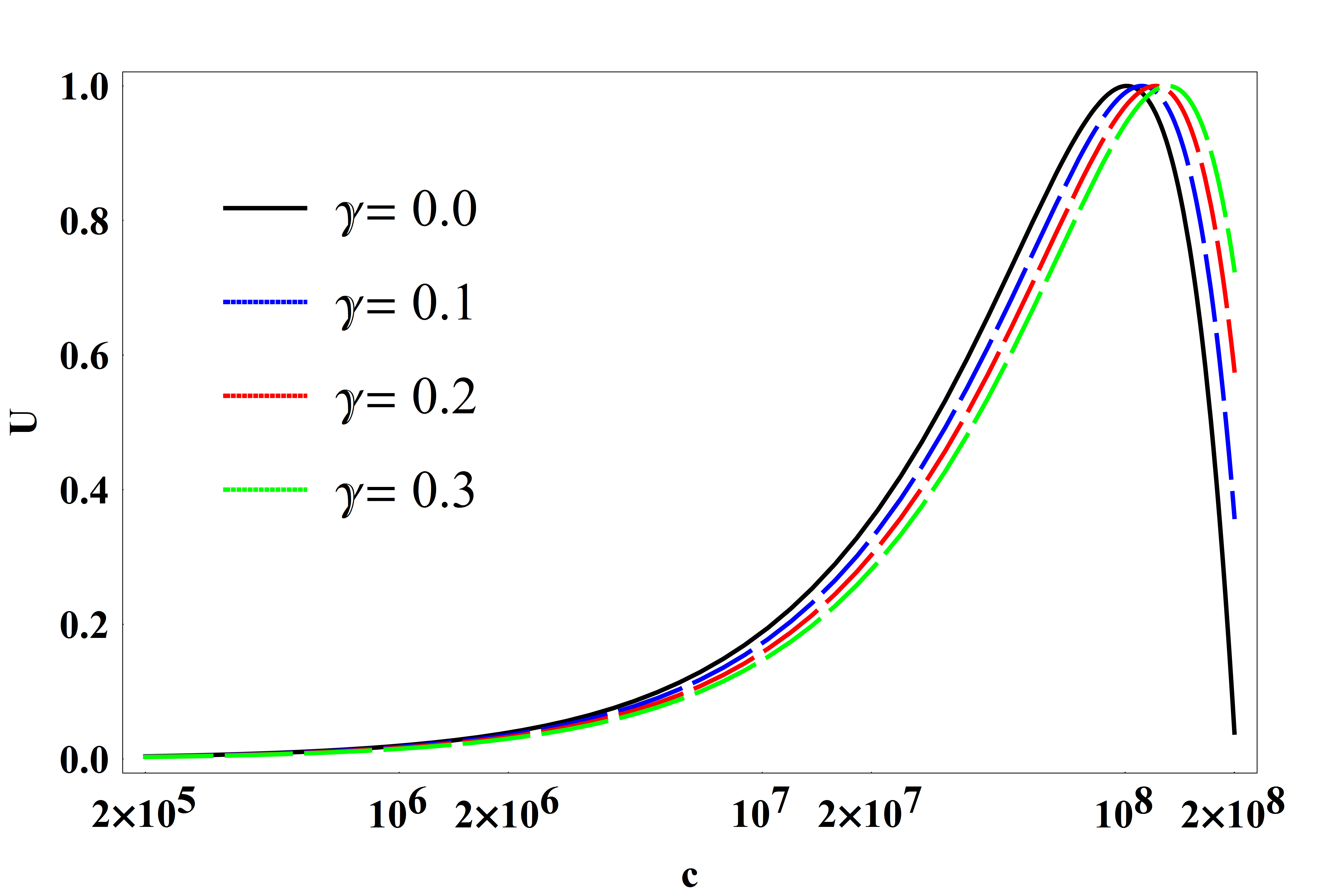
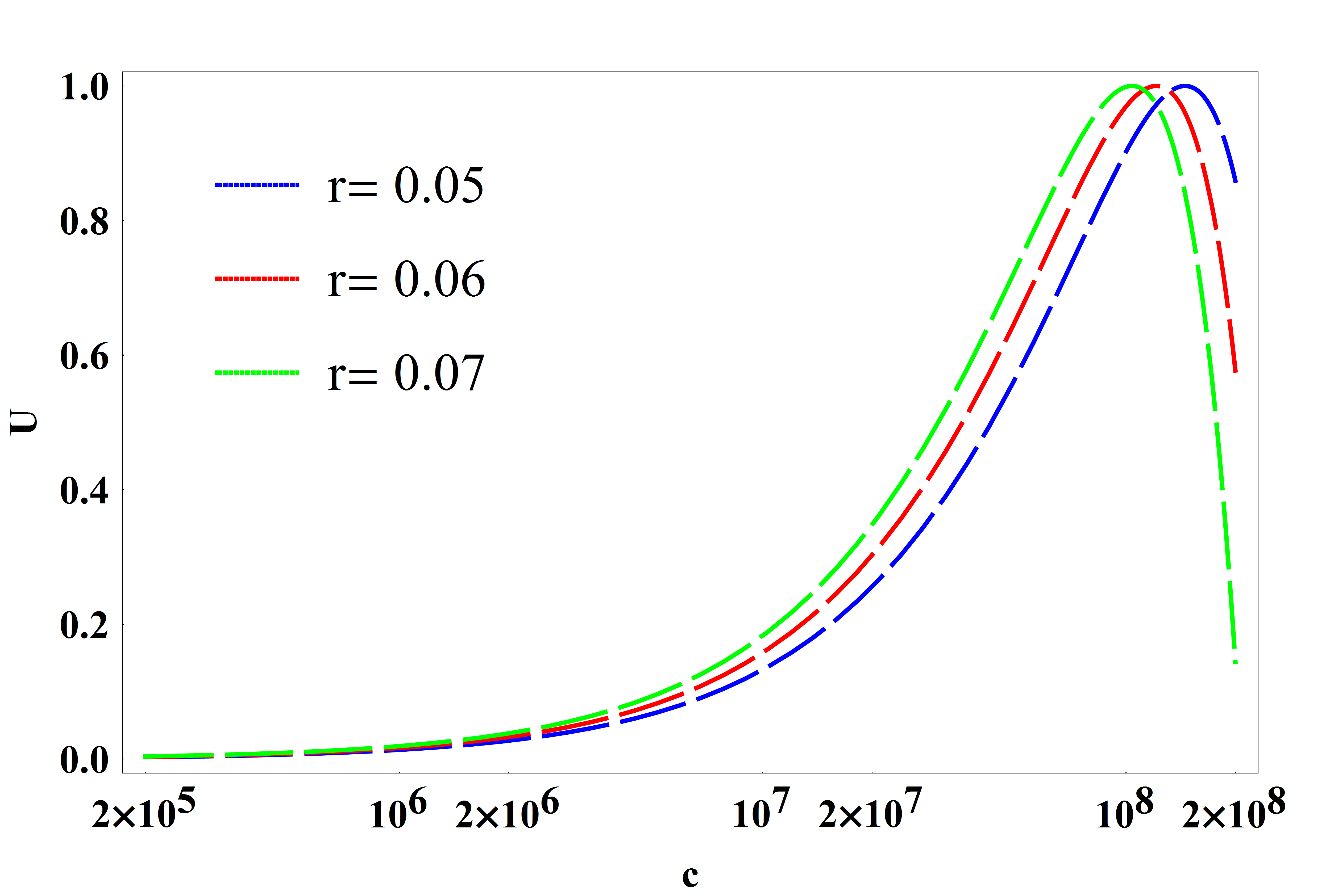
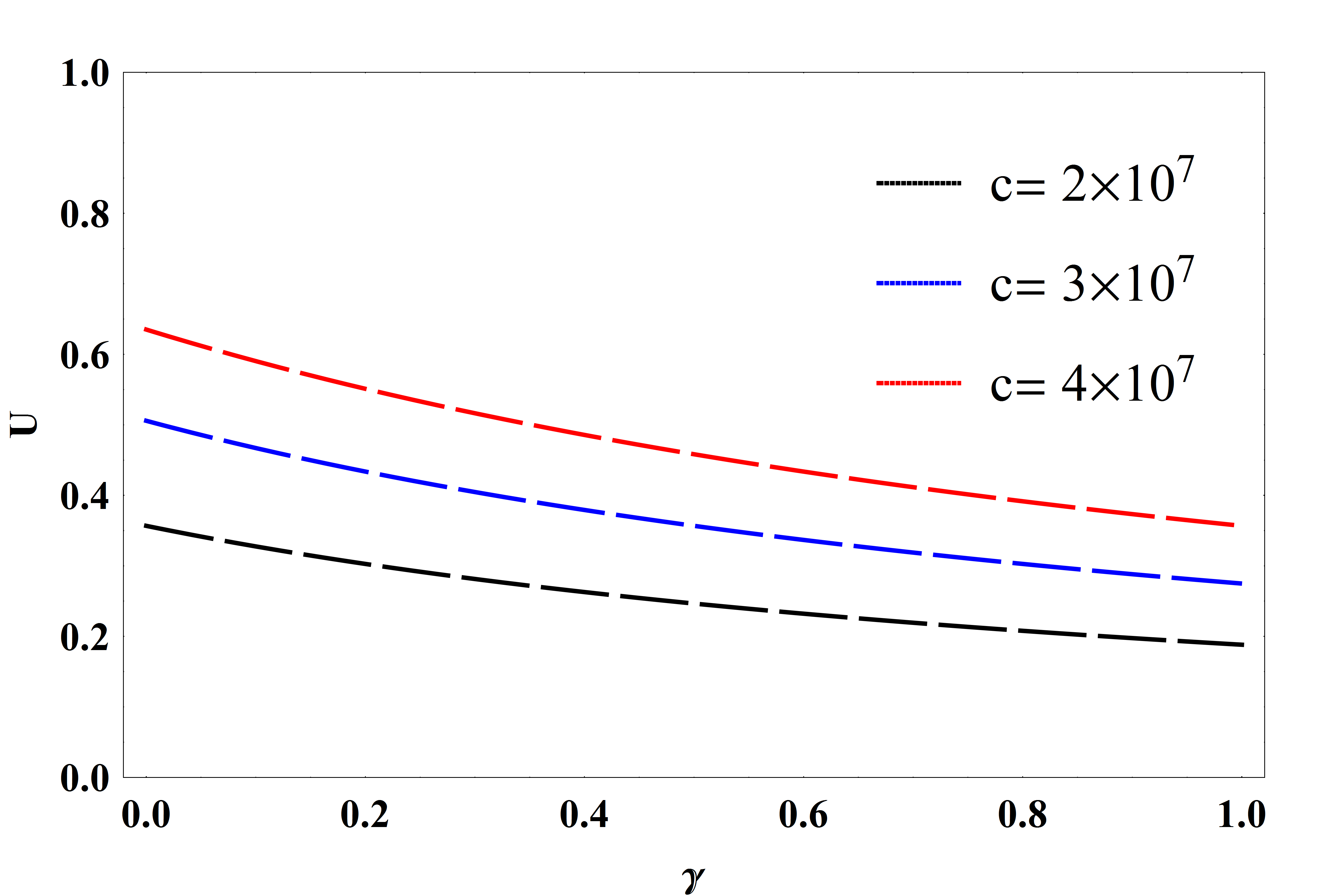
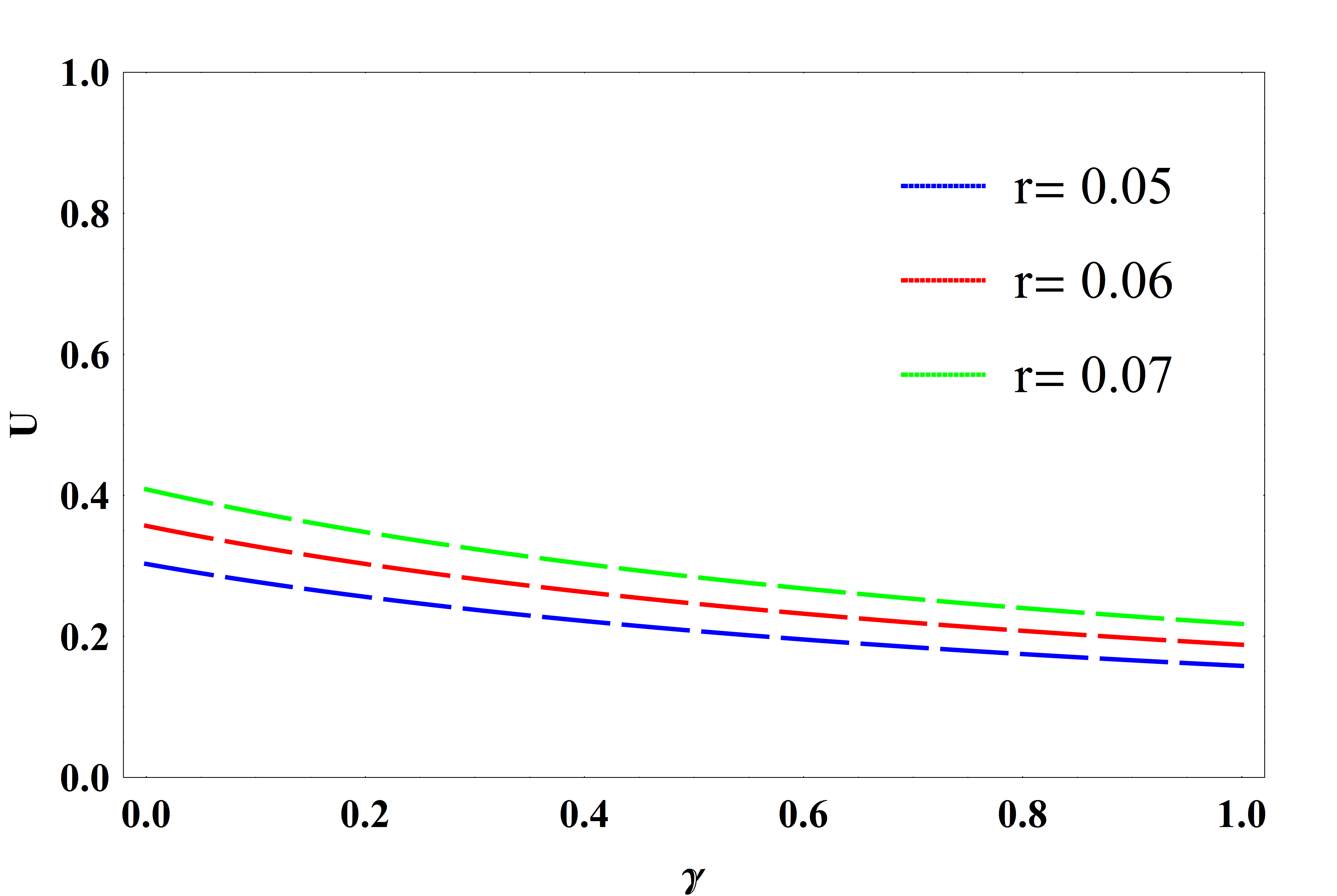
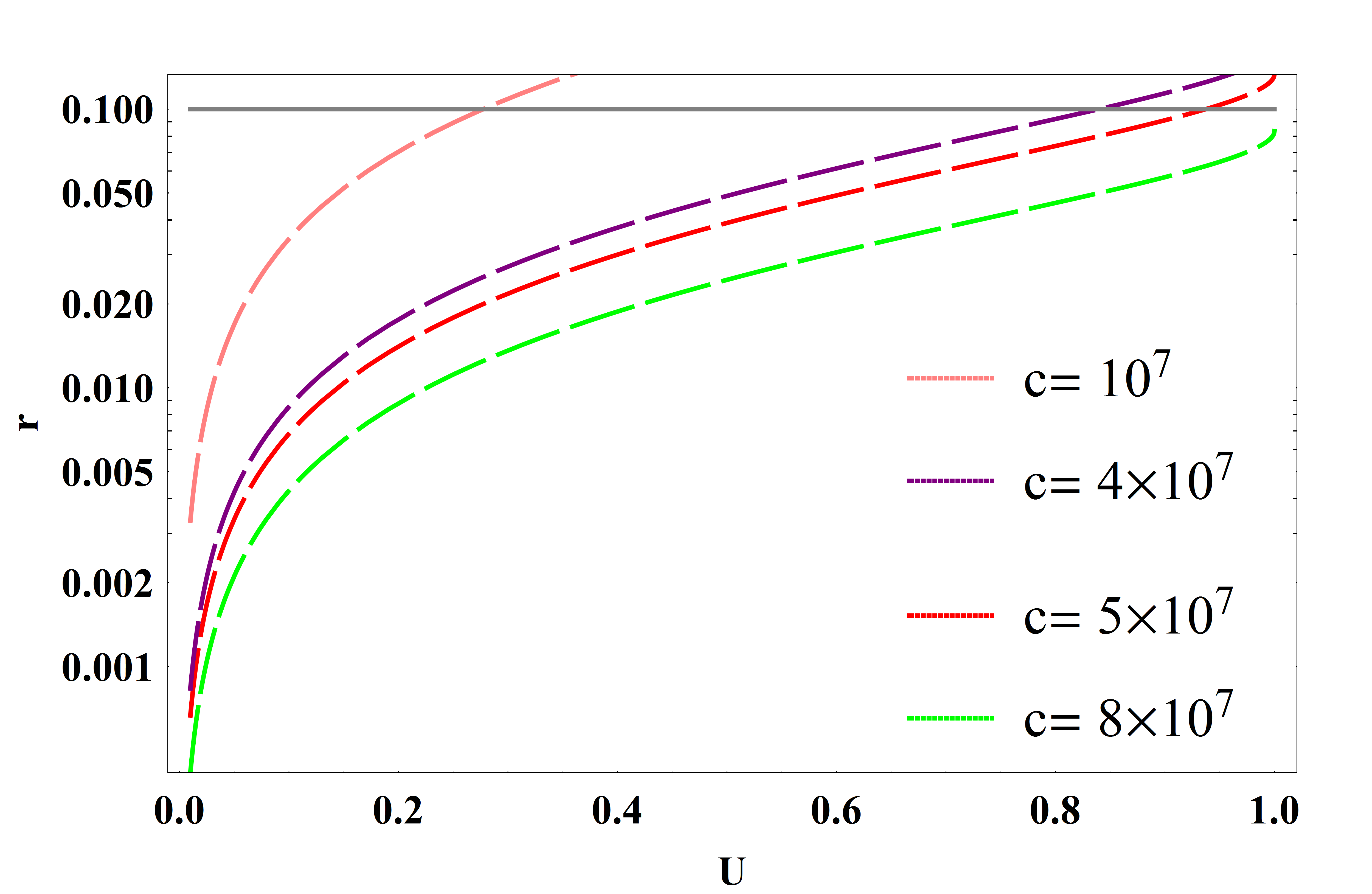
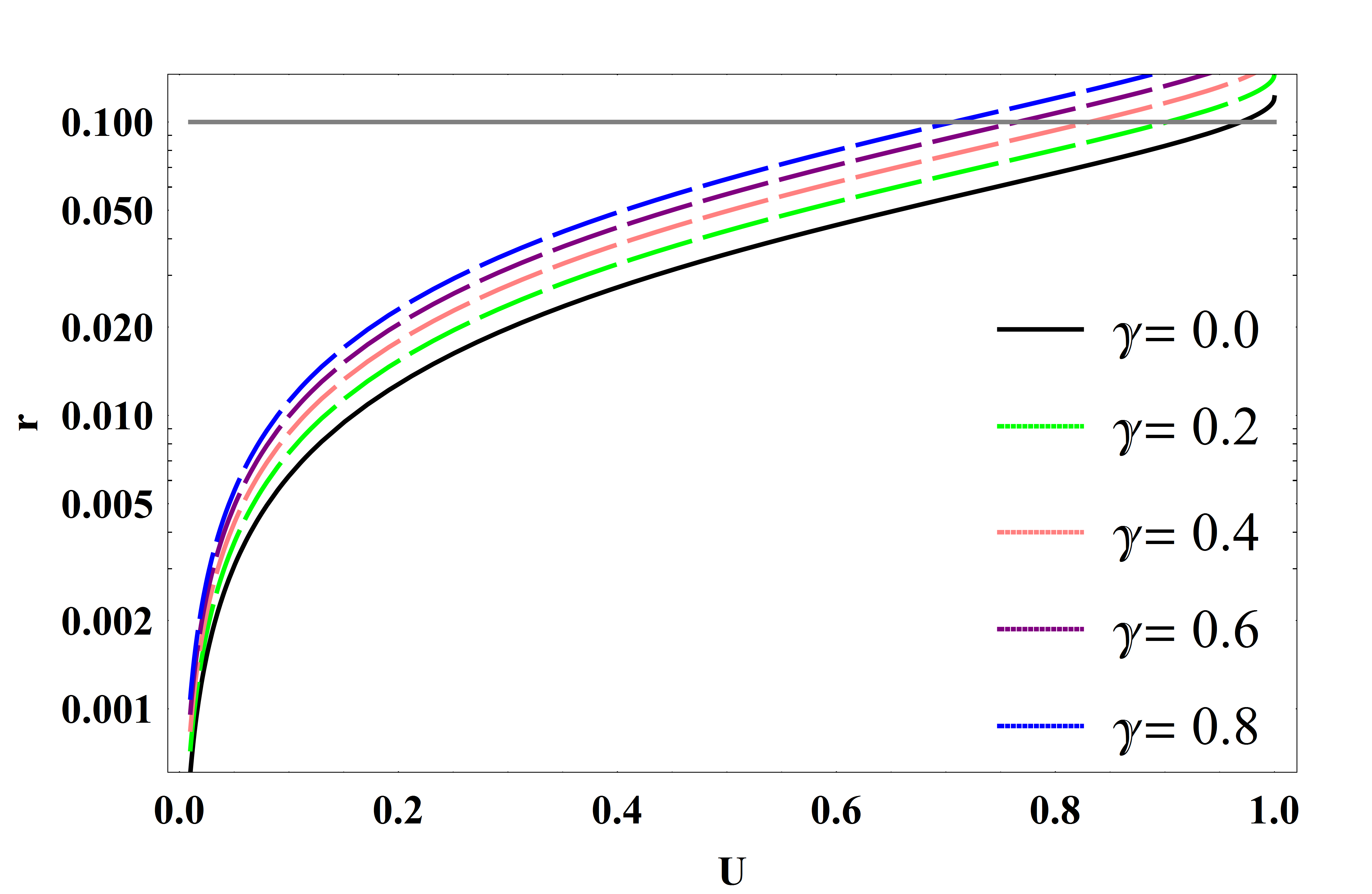
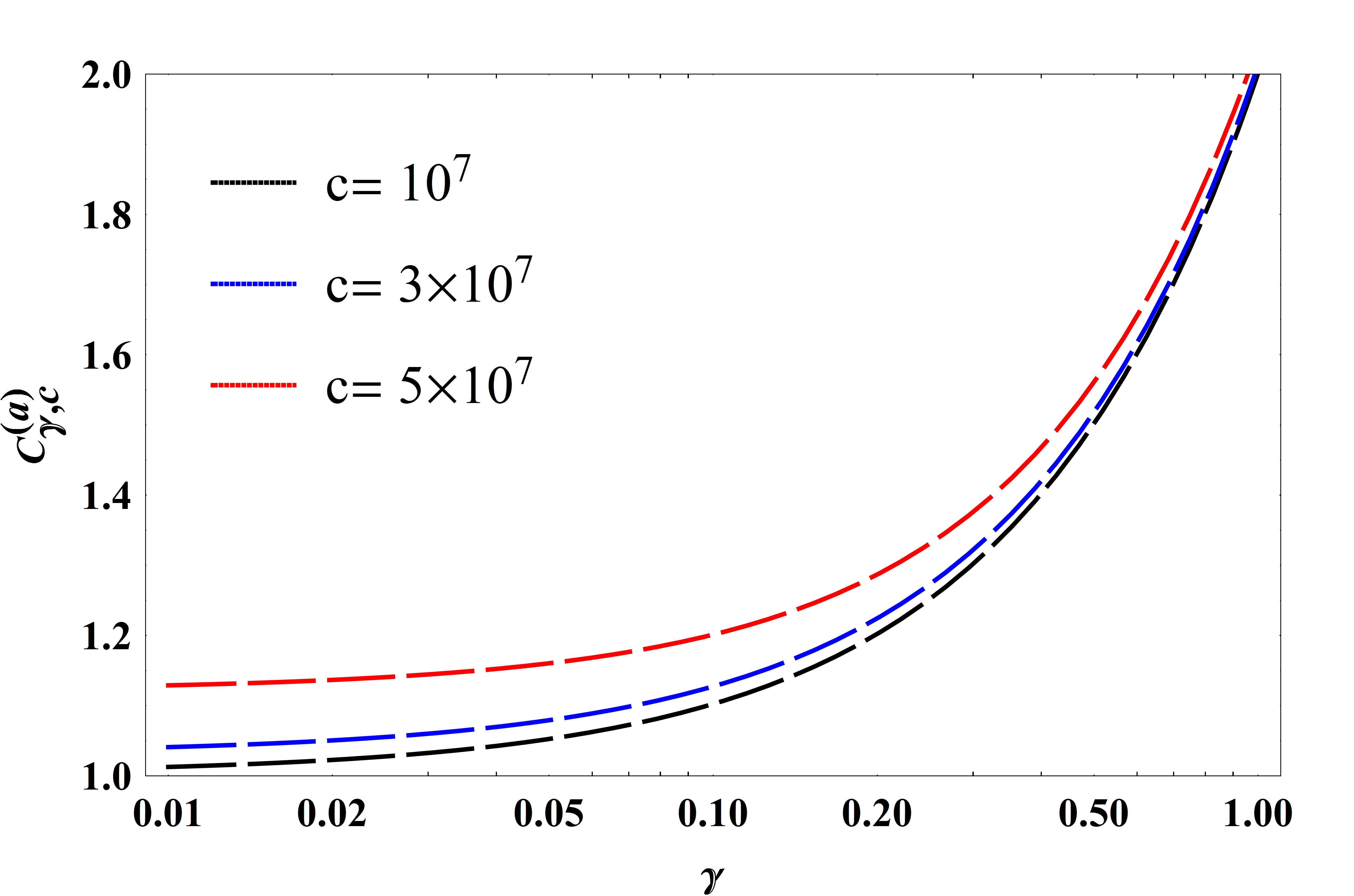
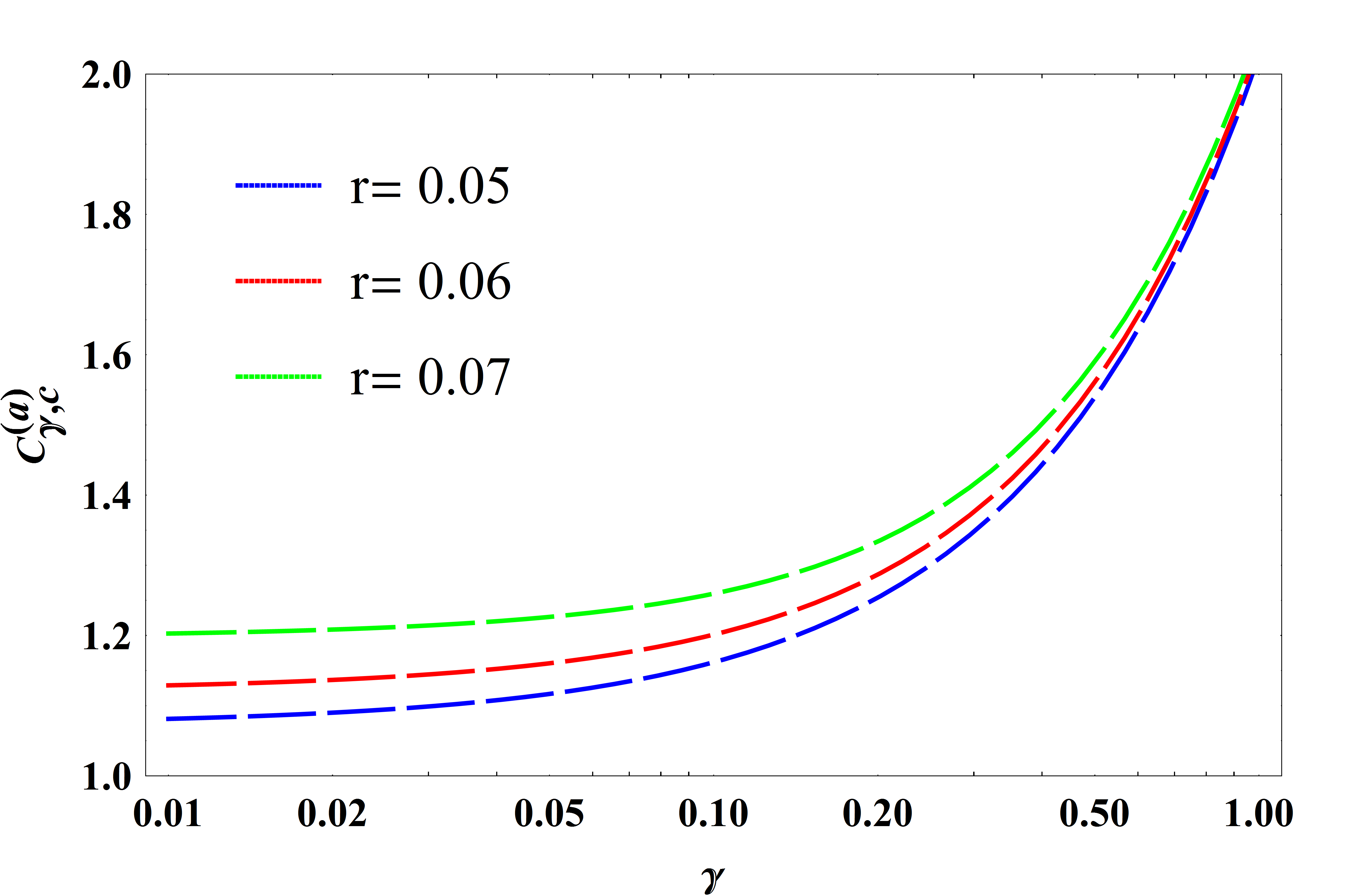
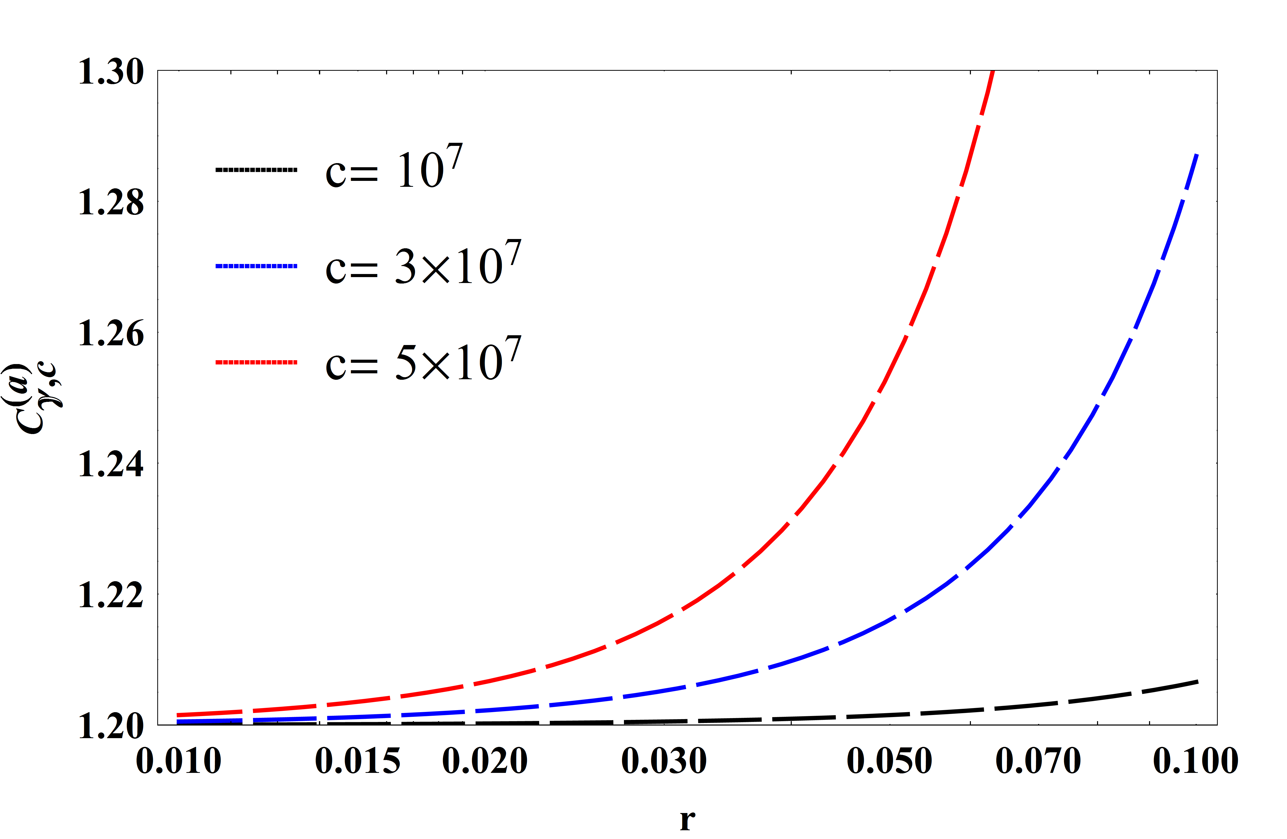
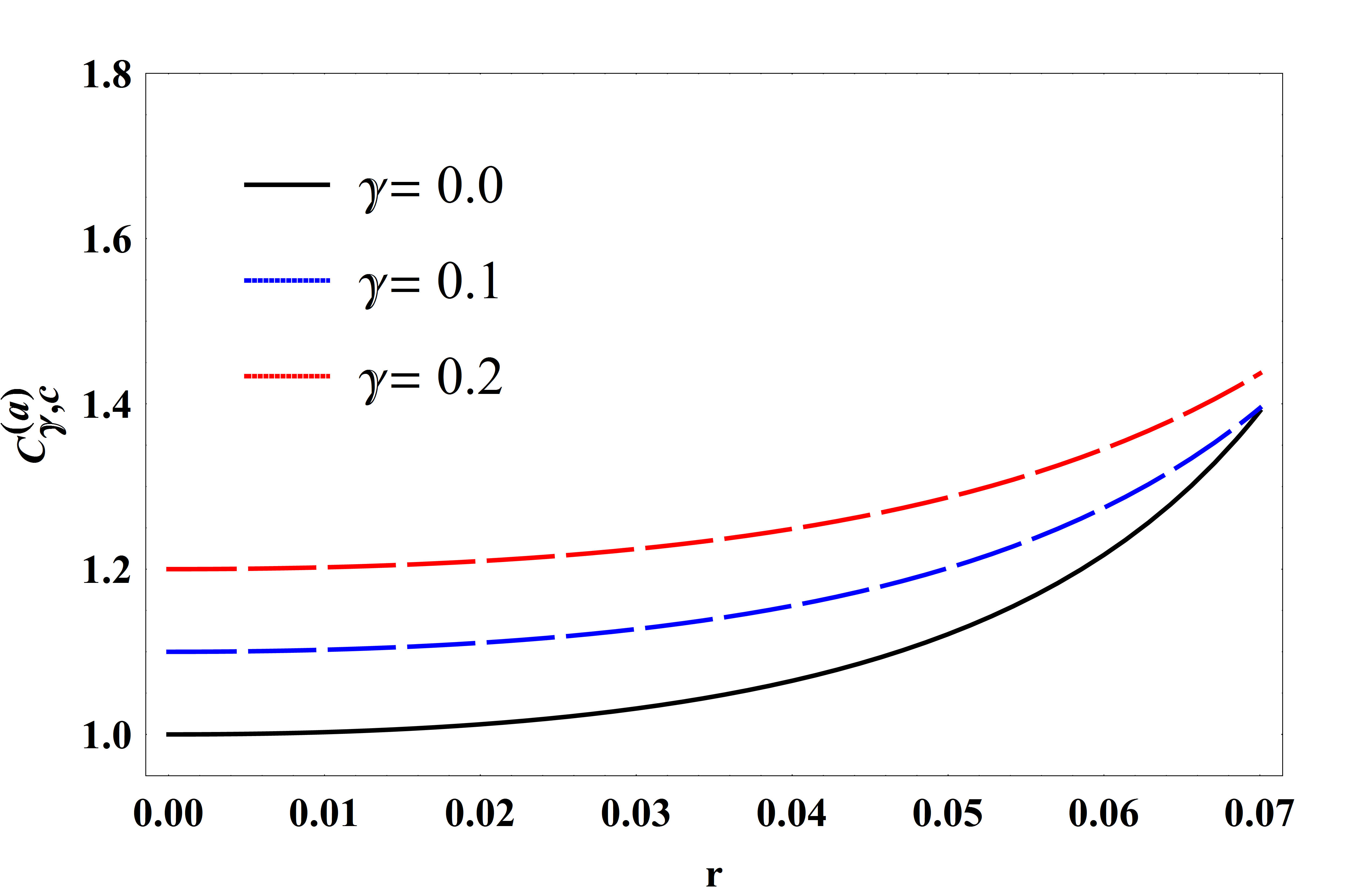
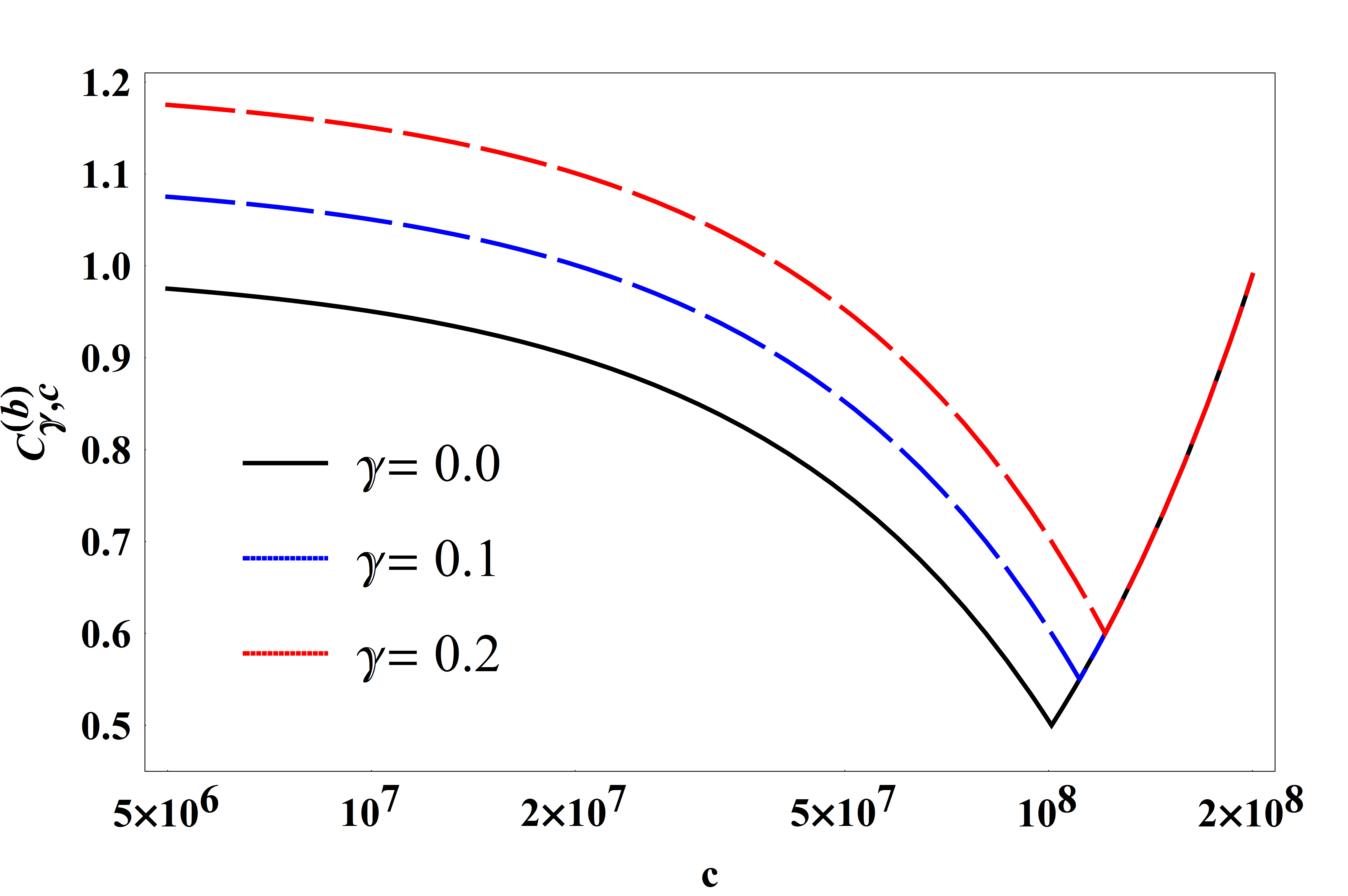
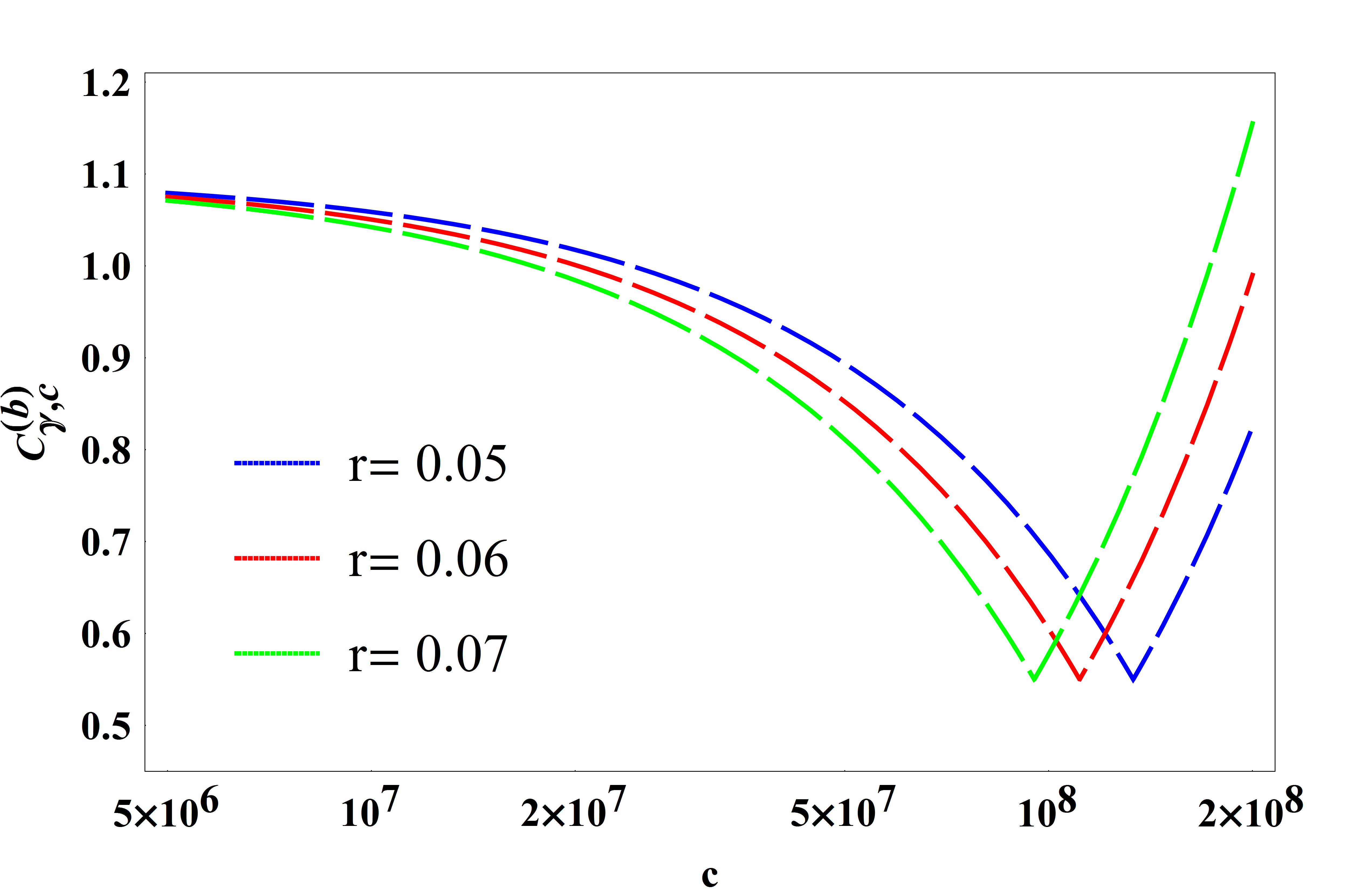
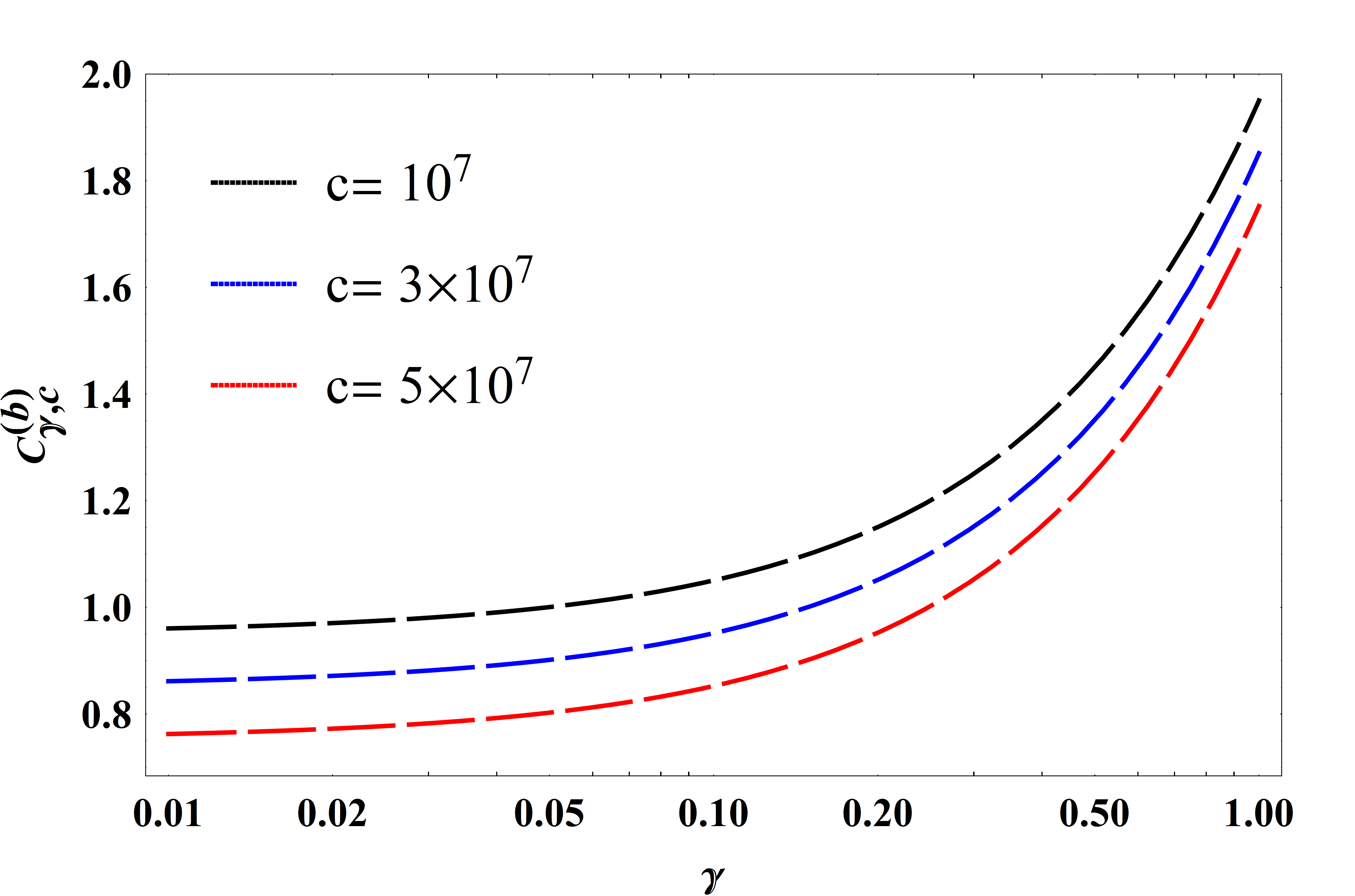
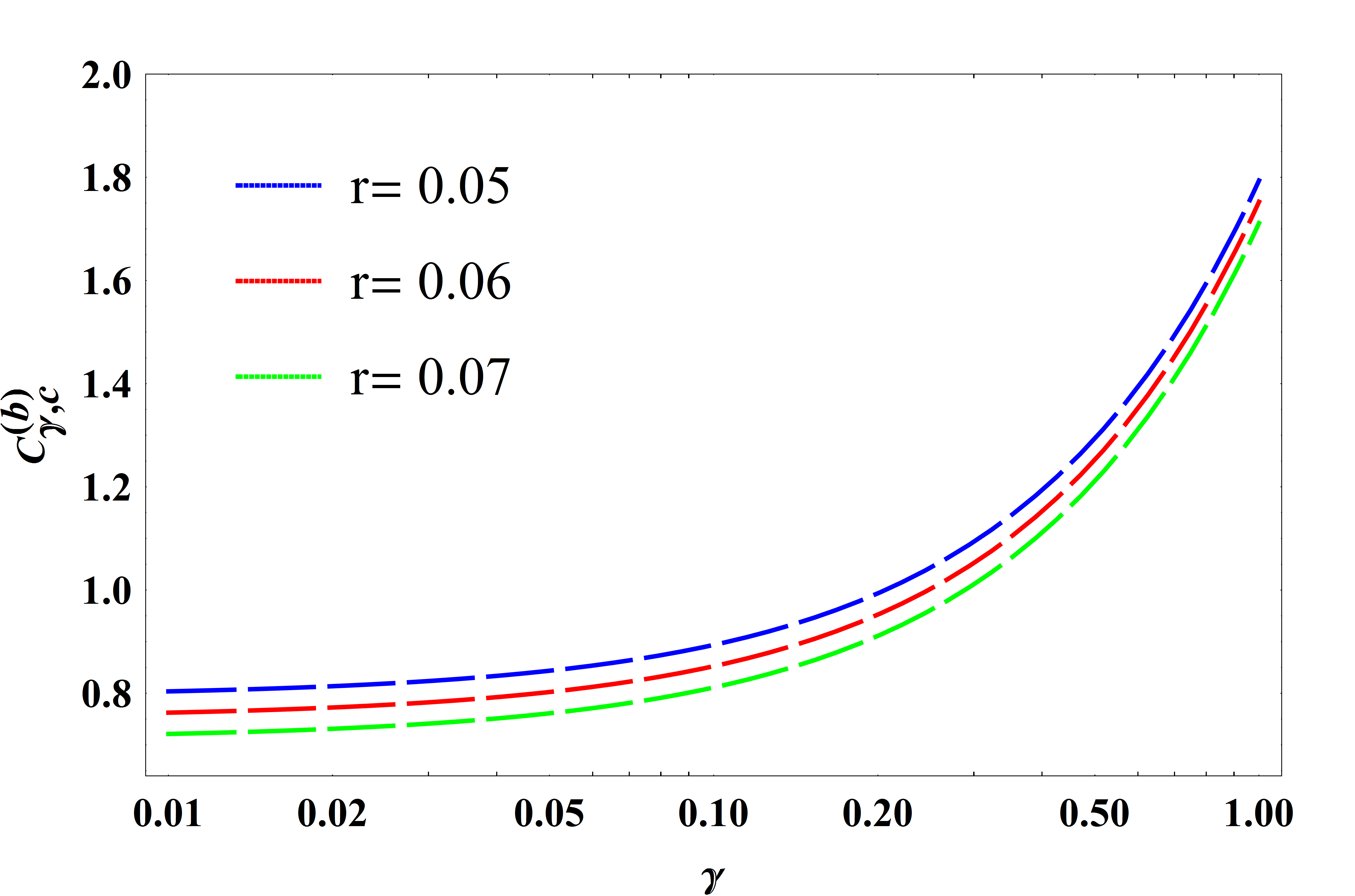
In Figures 1a-1d, we show the evolution of the dimensionless parameter Eq. (39) versus the conformal anomaly coefficient and the IG strength. We observe that the effect of the IG correction as well as the holographic cosmology starts from the values of the conformal anomaly coefficient , otherwise the holographic cosmology and the IG correction have no effect on the standard cosmology dynamics. Therefore, we plot the evolution of the tensor-scalar ratio versus the dimensionless parameter , Figs. 1e and 1f, in the range . From these two figures we notice that the predicted values of the tensor-scalar ratio are included in the bound imposed by Planck data Akrami:2018odb .
From now on we will consider the range for the conformal anomaly coefficient in order that holographic cosmology can leave its imprints on the spectrum of the gravitational waves.
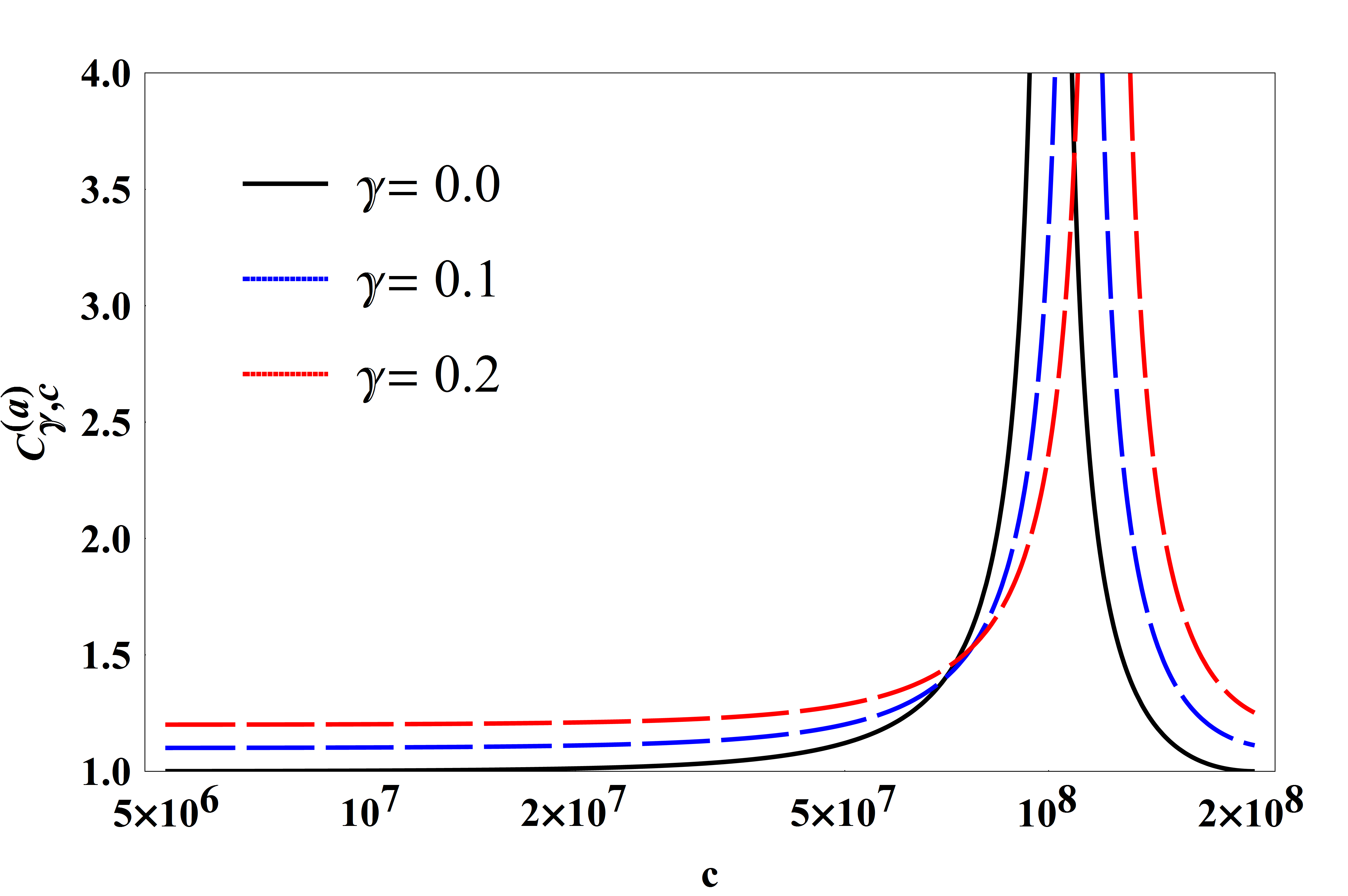
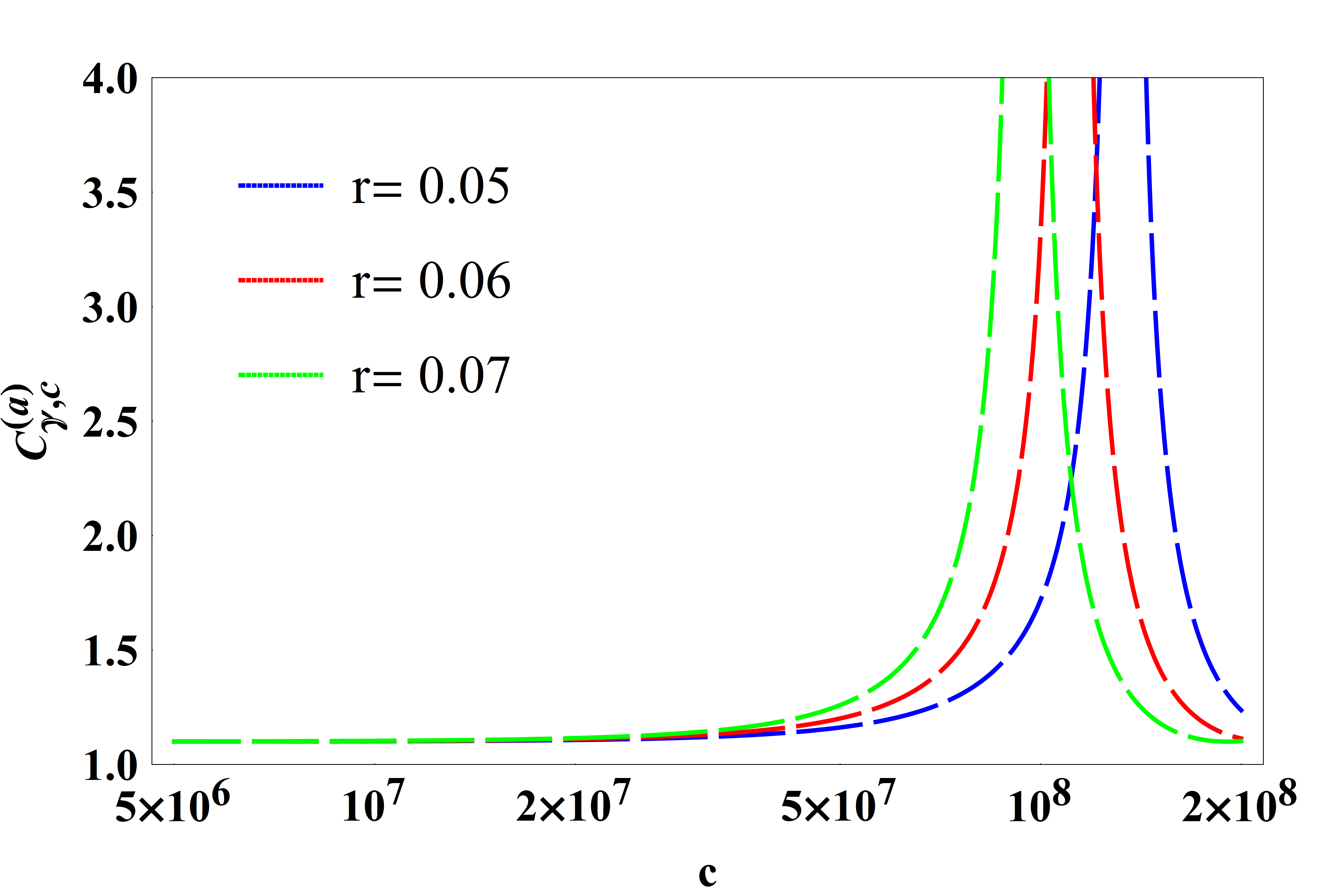
The behavior of the correction terms and is shown in Fig. 2 and Fig. 3 respectively. From these figures we see that the effect of the holographic cosmology appears only for the values which confirms the aforementioned conclusion about the range of . The maximal value of the conformal anomaly coefficient corresponding to is reflected by the maximum of the correction term which is not defined (see Fig. 2a) and by the maximum of which is equal to for (see Fig. 3a). We notice also from Figs. 2 and 3 that for , we can always find a range of the conformal anomaly coefficient in which the effect of the IG is appreciable.
III.2 Scalar inflation with quadratic potential
In this subsection, we begin by specifying the functional form of the potential in order to calculate the spectrum of density perturbations and of gravitational waves, and then check their consistency with observations. Here we will consider the quadratic scalar potential given by the following expression
| (41) |
where is a dimensionless parameter. By substituting the quadratic potential Eq. (41) in Eq. (15), the number of e-folds reads to
| (42) |
By using equations (30) and (41) we rewrite the slow-roll parameter as
| (43) |
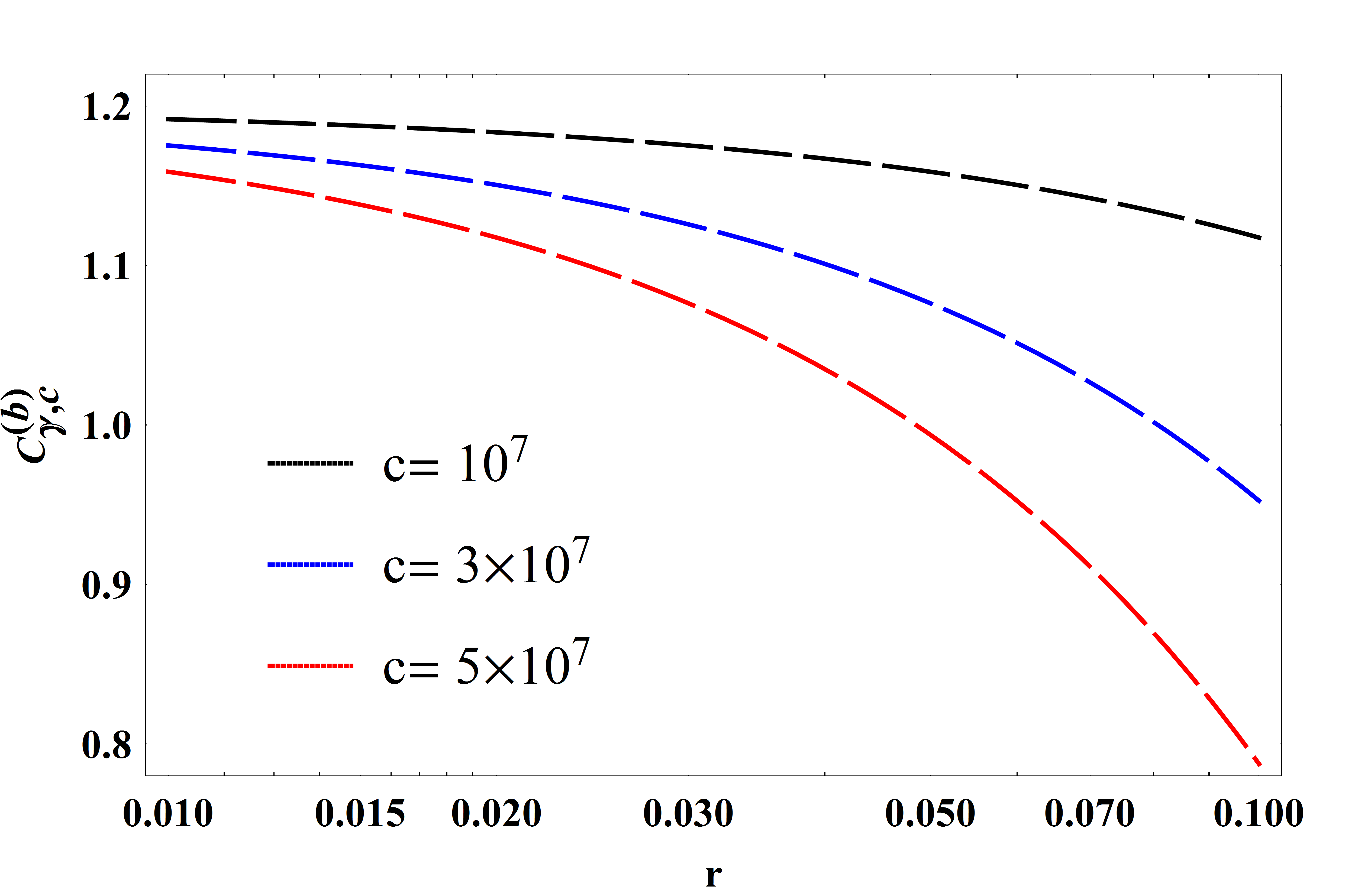
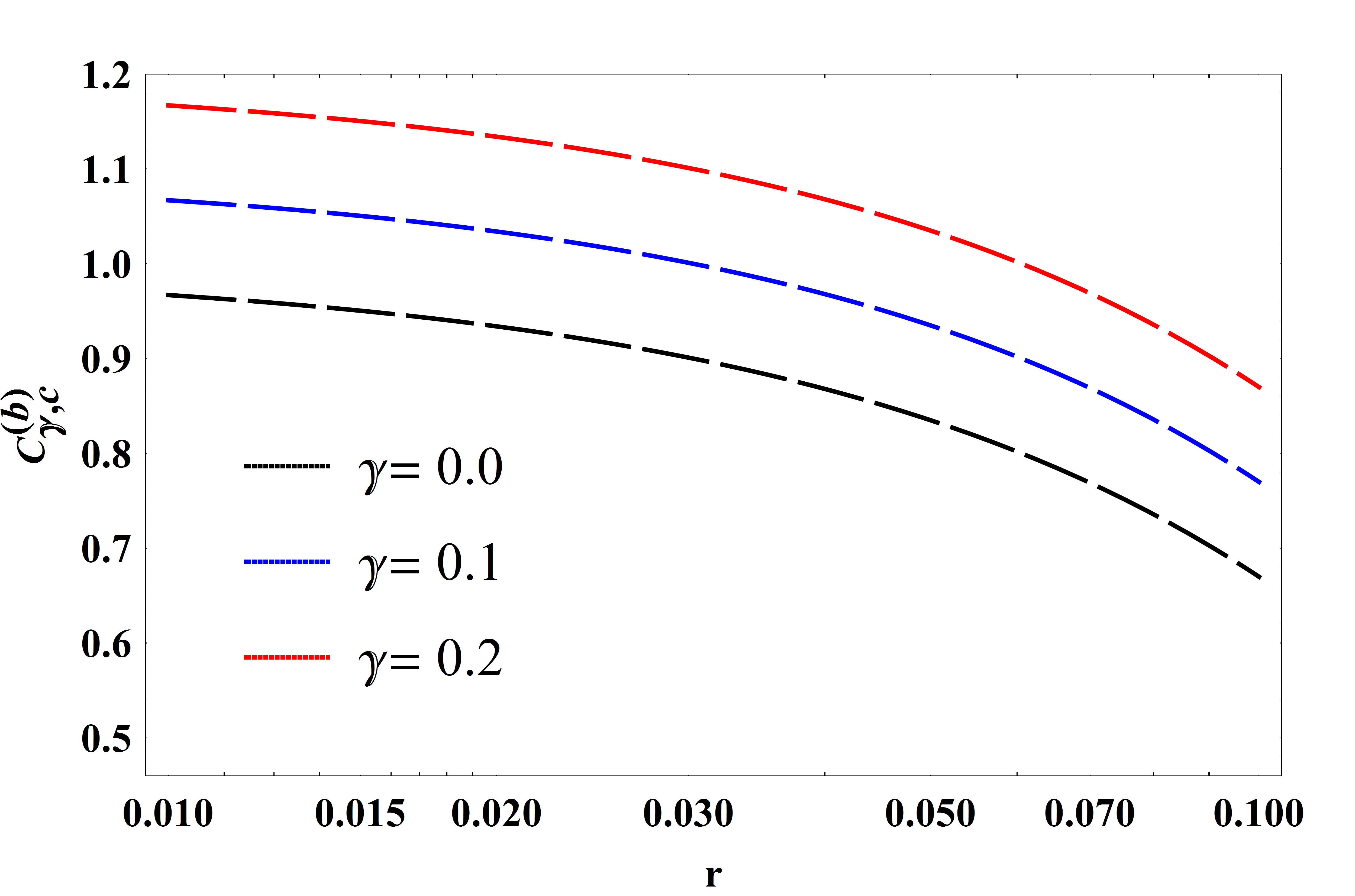
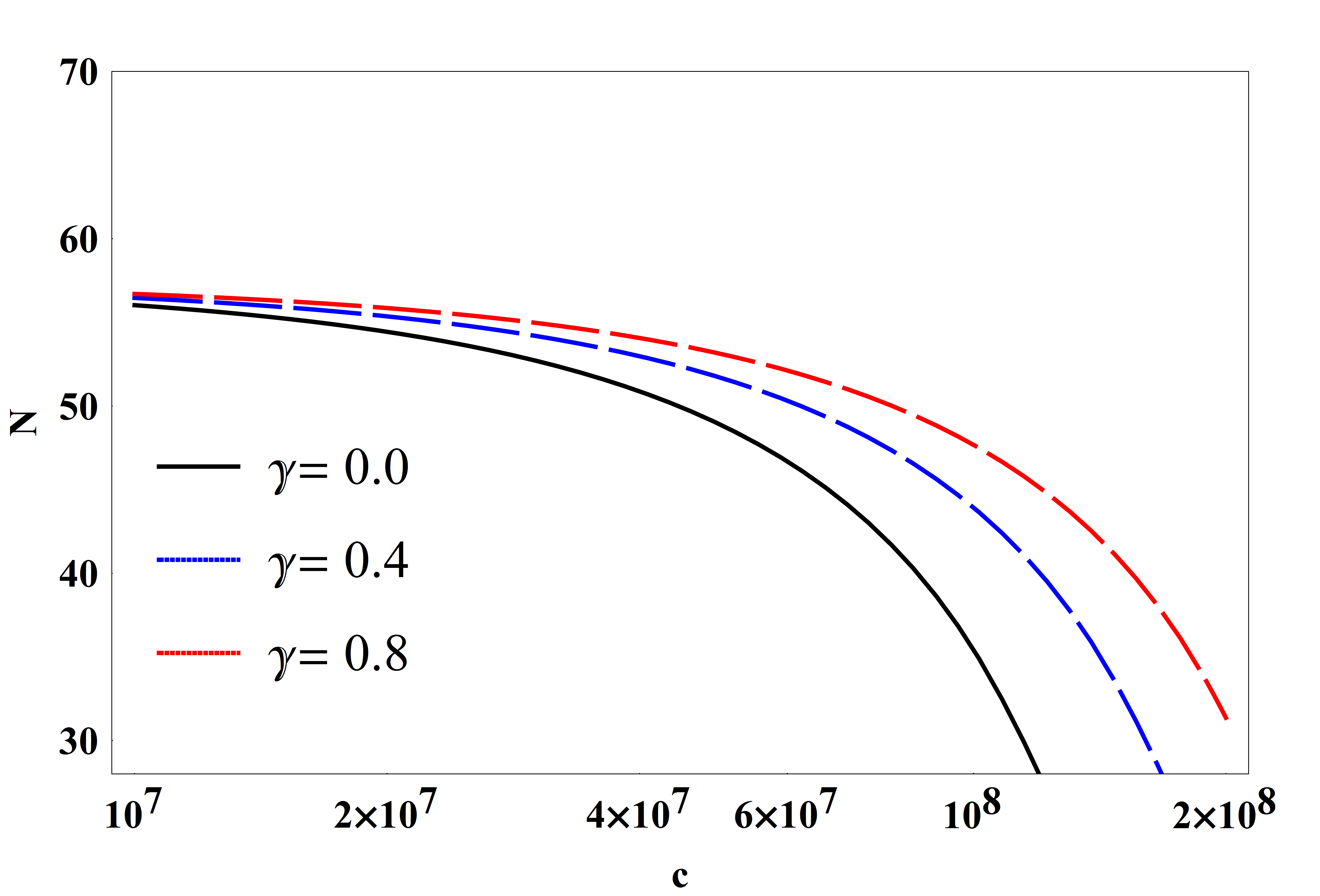
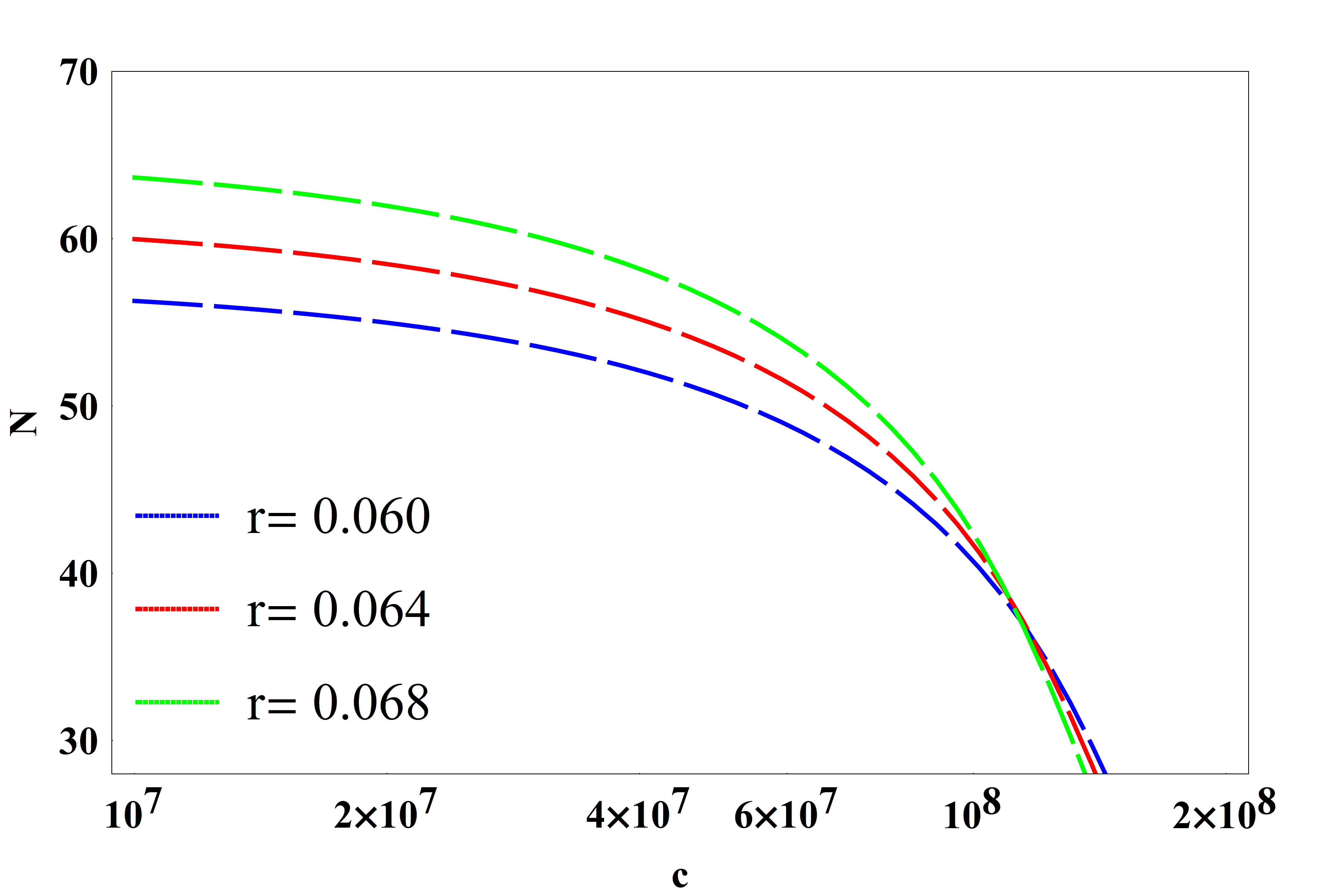
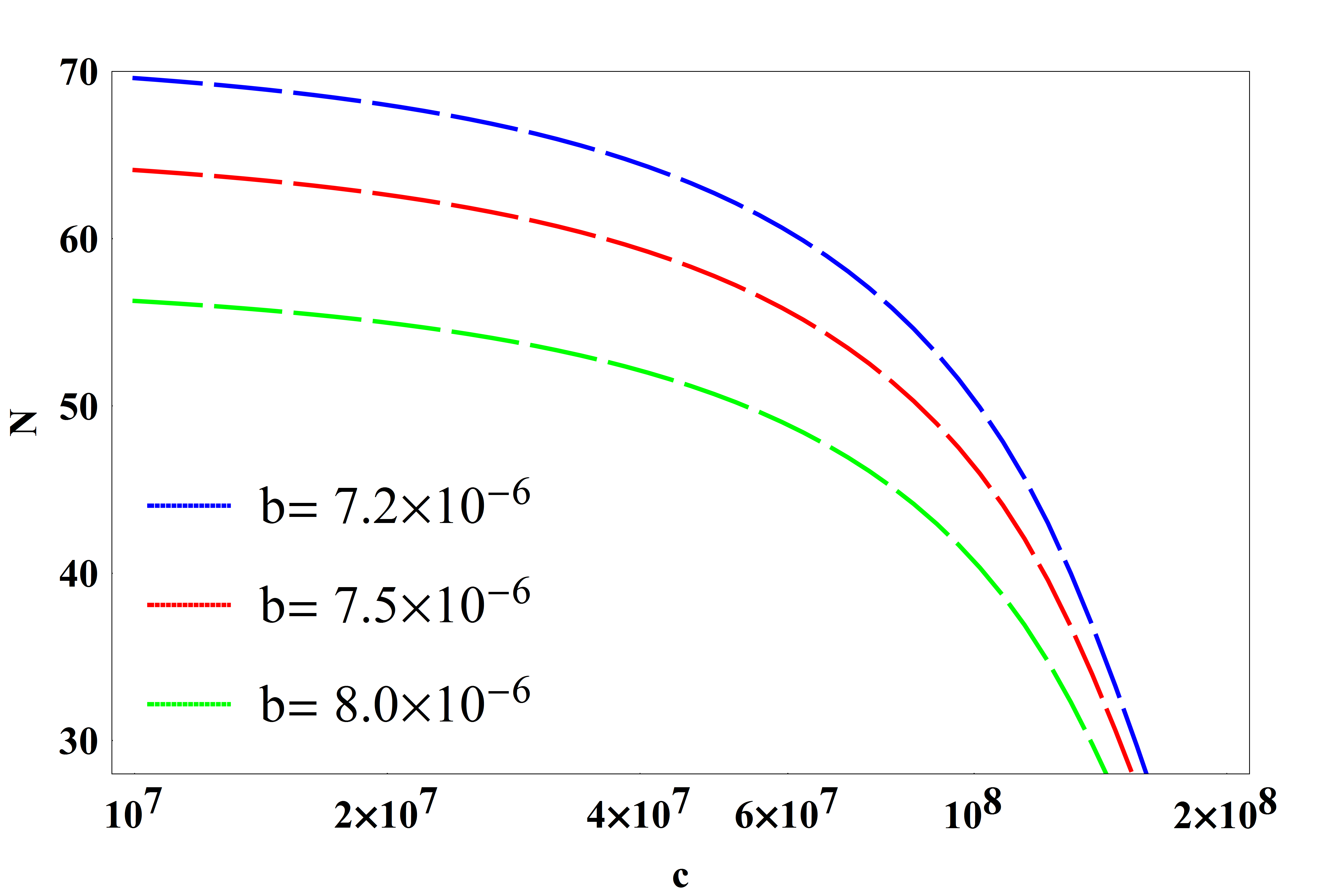
Inflation breaks down at and at the low energy limit we find , i.e. which recovers the standard form of the scalar field for a quadratic potential at the end of inflation UrenaLopez:2007vz . Fig. 4 shows the evolution of the number of e-folds against the coefficient . In Figs. 4a, 4b, 4c, the plot is for different values of the IG strength (, ), different values of the tensor to scalar ratio (, ) and for different values of the parameter (, ) respectively. We conclude from these figures that for the number of e-folds is in the range which is in good agreement with observations.
From Eq. (18), we derive the scalar perturbation at the crossing horizon as
| (44) |
The scalar spectral index Eq. (19) at the crossing horizon is given by
| (45) |
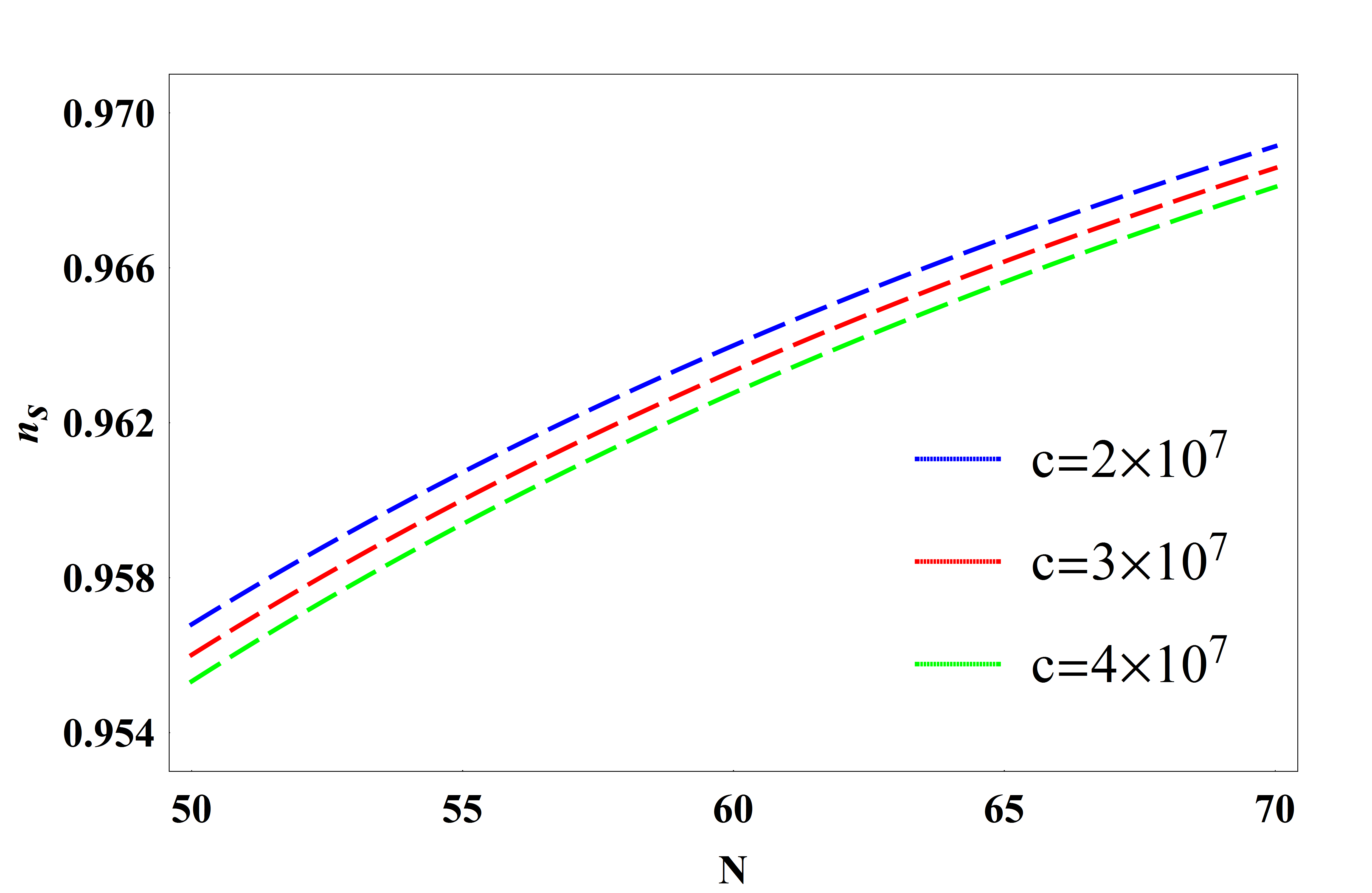
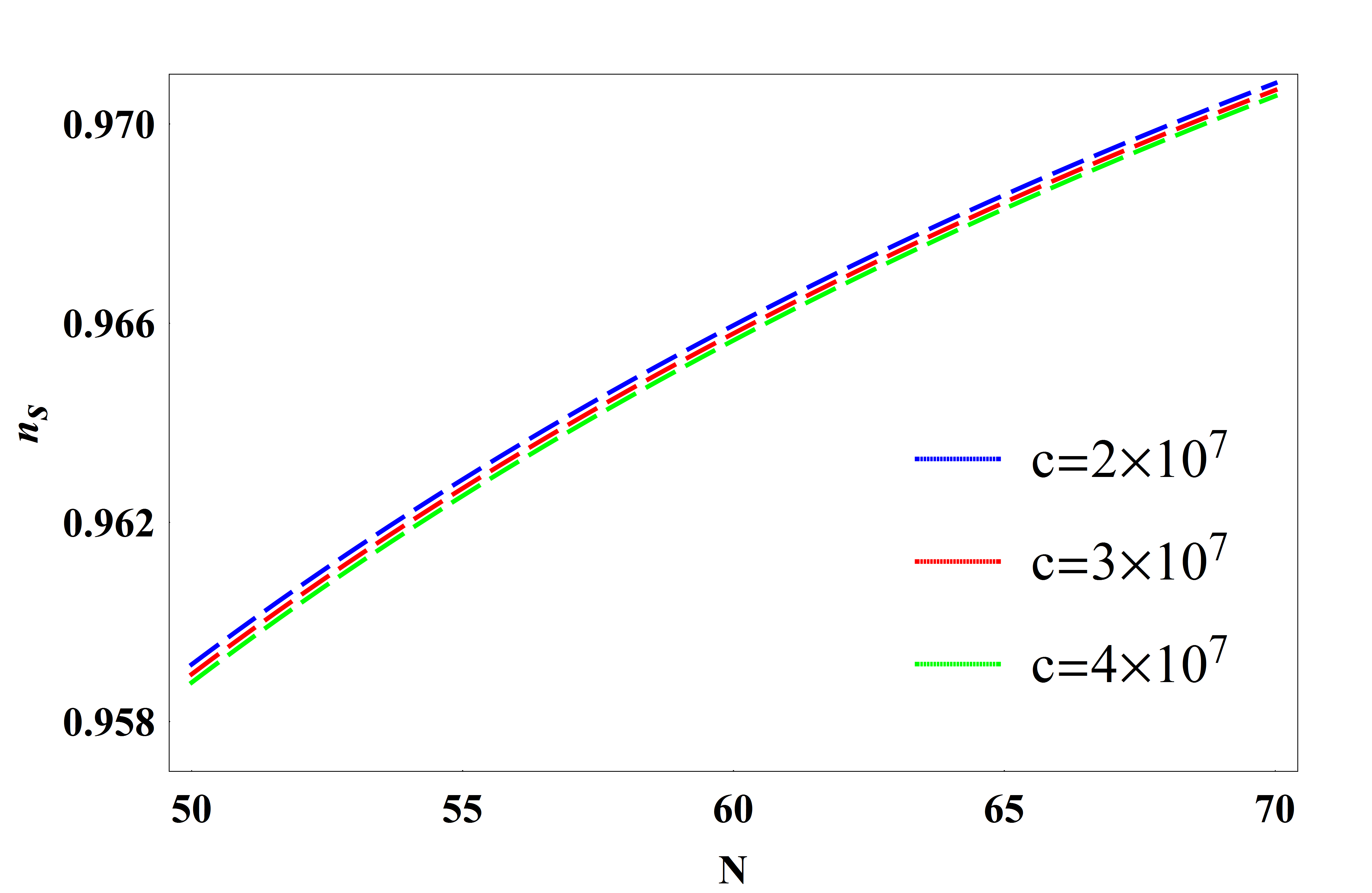
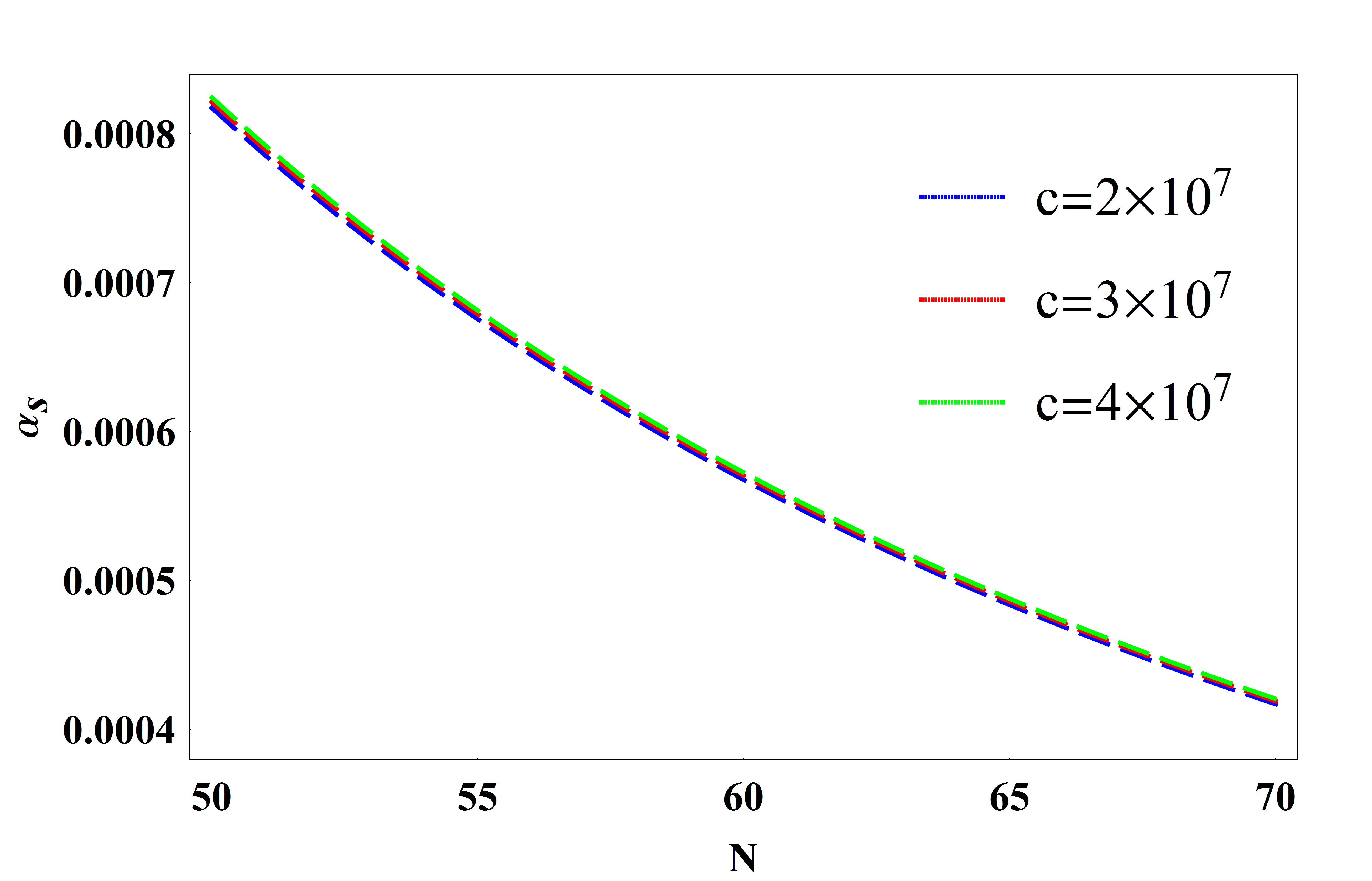
Figure 5a shows the variation of the scalar spectral index versus the number of e-folds, for different values of the conformal anomaly coefficient for , and . The running of the spectral index defined as can be expressed using Eq. (42) and Eq. (45) as
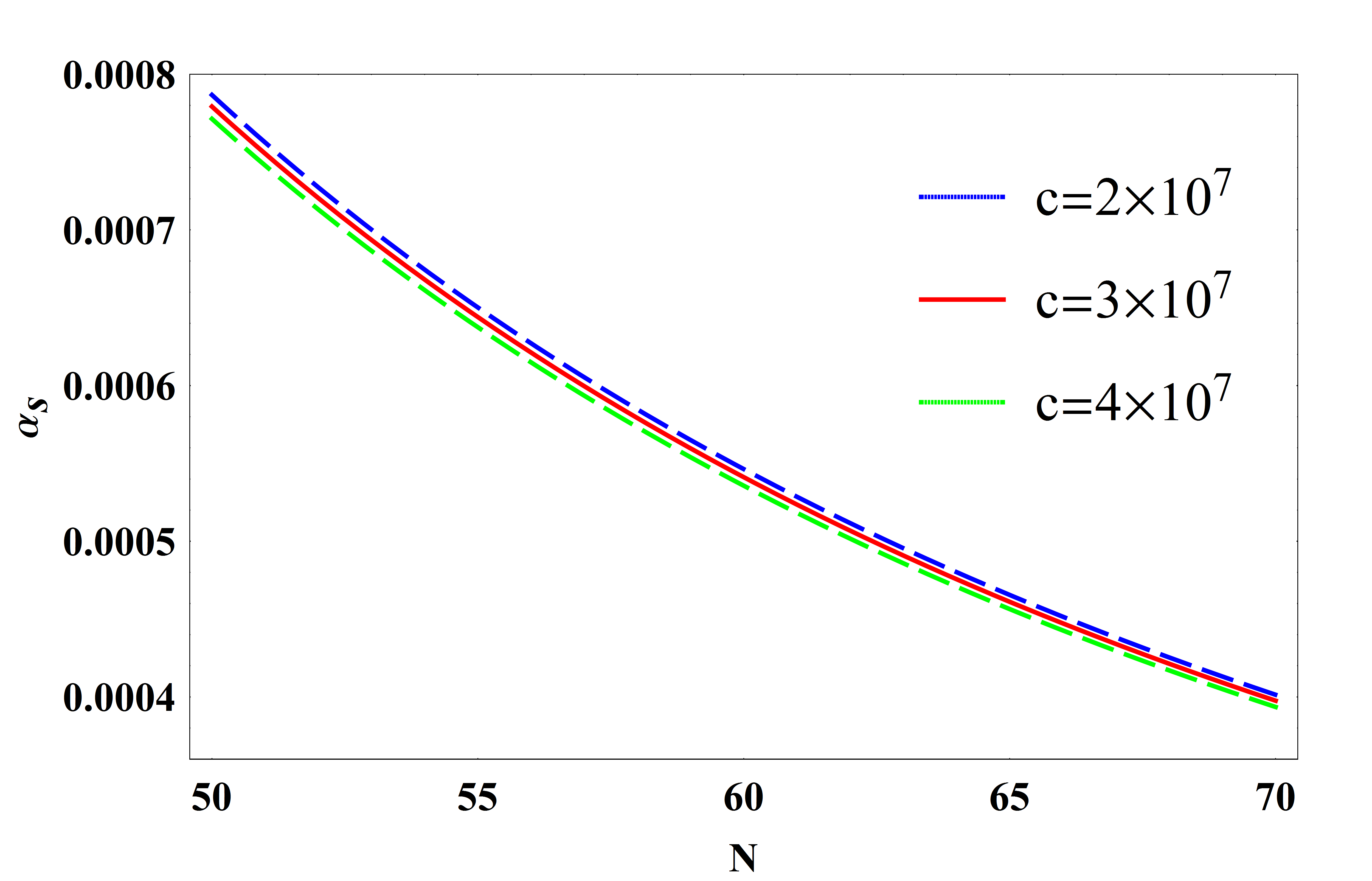
| (46) |
In Fig. 5b we show the evolution of the running versus the e-folding number , for different values of the conformal anomaly coefficient for , and . One can see from Figs. 5a and 5b that for the scalar spectral index and its running are consistent with the Planck 2018 data Akrami:2018odb .
In Table. 1, we have summarized the predicted and the observed inflation parameters making use of Figs. 5a and 5b. These results are well supported by the Planck 2018 data.
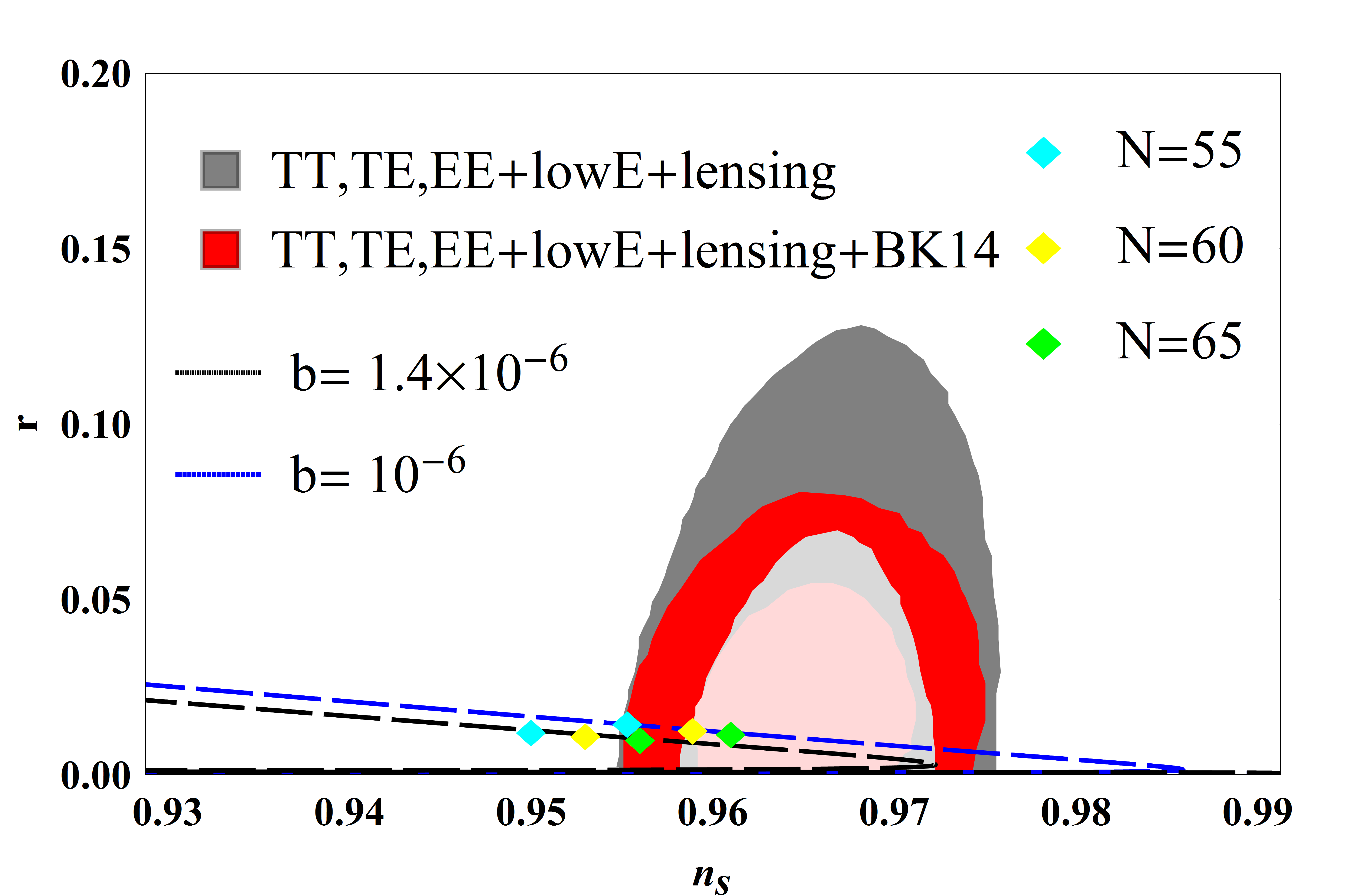
Finally, the ratio between the amplitudes of tensor and scalar perturbations at the crossing horizon is given by
| TT,TE,EE+lowE+lensing | |||||
|---|---|---|---|---|---|
| (47) |
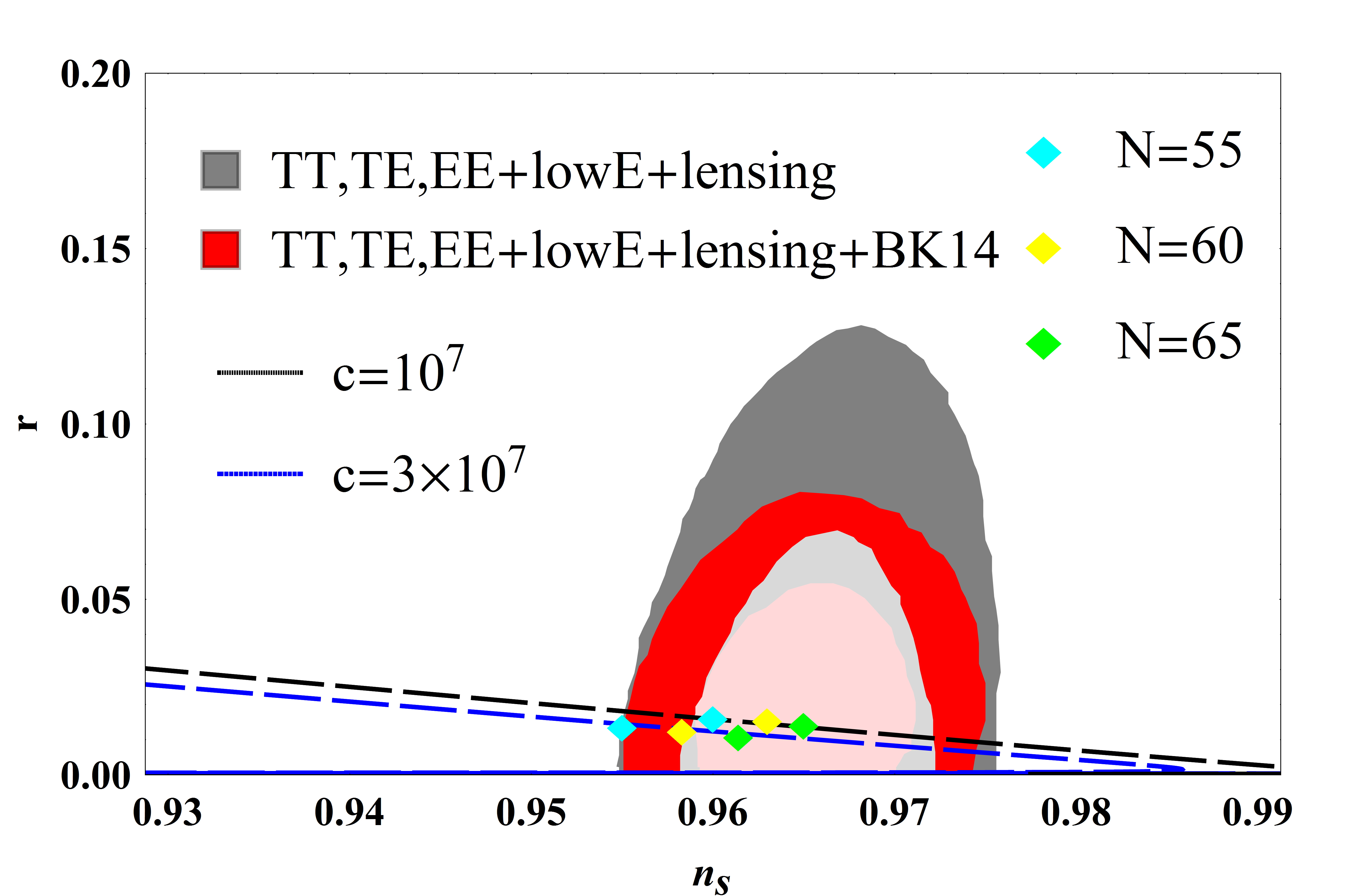
Figures 6a, 6b and 6c show the contour plot for different values of , and , in comparison with the observational data. The gray contour comes from the Planck TT, TE, EE, lowE+lensing data while the Planck TT, TE, EE, lowE+lensing+BK14 data are included in the red contour. The black and the blue dashed lines represent the theoretical predictions. One can see that the predicted parameters of the model lie within the C. L. region. In this figure we have highlighted three values of that are in the range . Moreover the parameter used in our plots lies in the range estimated by the authors in Ref. UrenaLopez:2007vz .
III.3 Tachyonic inflation with an exponential potential
In this subsection we adopt the exponential potential given by
| (48) |
where is a dimensionless parameter. This type of potential arises naturally from fundamental theories such as String theory/M theory tch . With the aid of Eq. (48) and by using Eq. (15) the number of e-folds for the tachyon field yields
| (49) |
The slow roll parameters becomes
| (50) |
at the end of inflation (), we find that at low energy, . This gives which is the same as the standard one Sami .
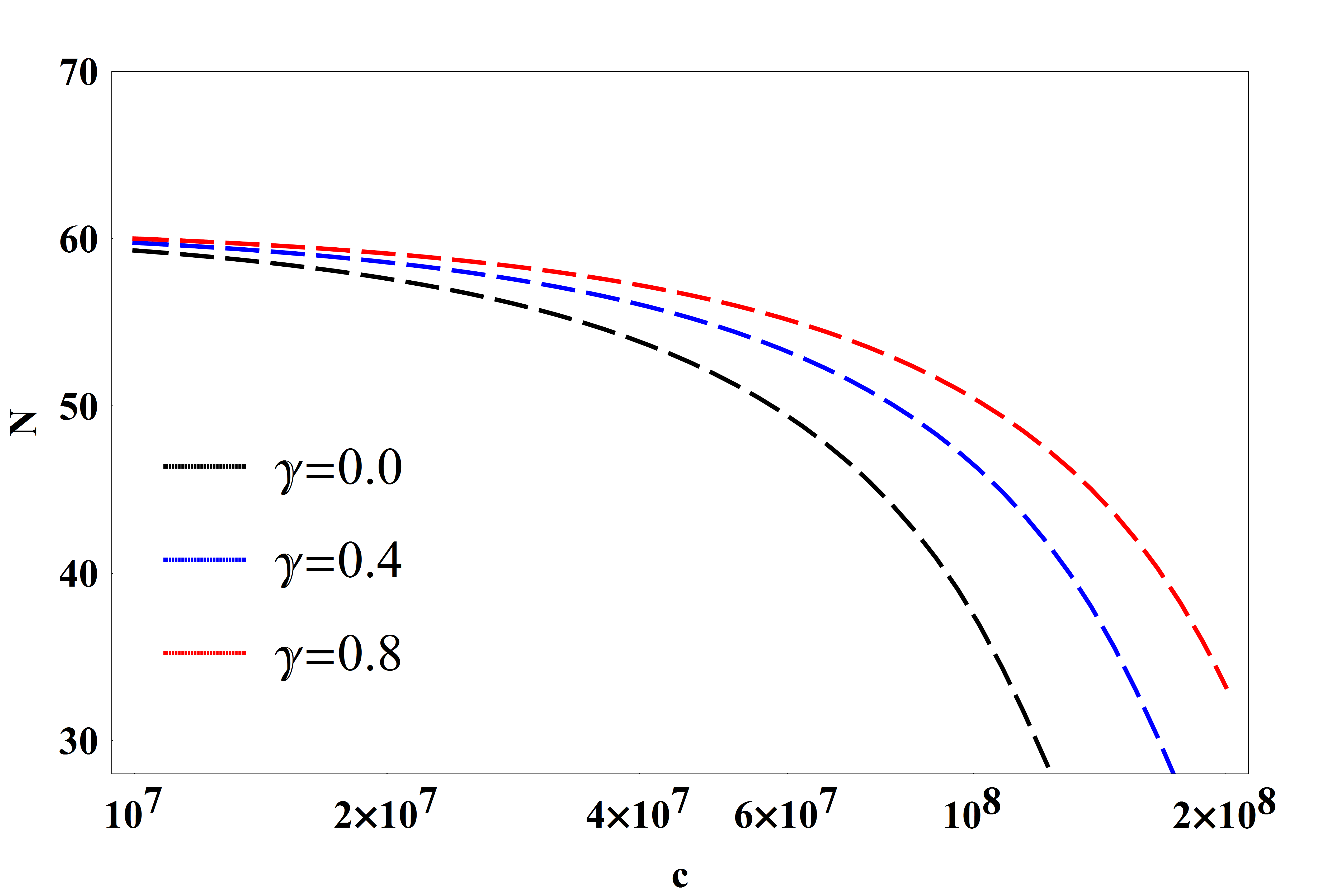

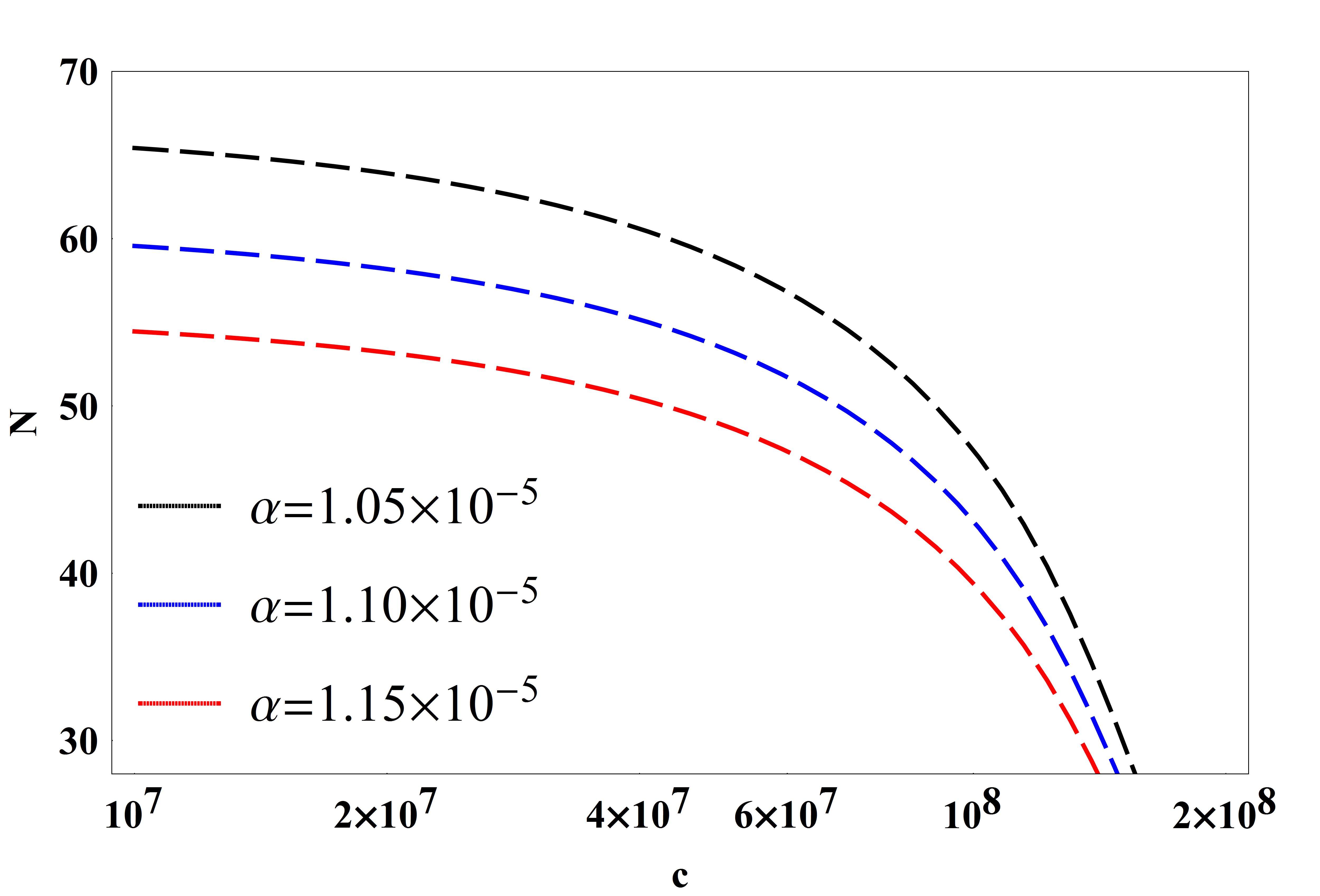
Similarly, Fig. 7 shows the variation of the e-folding number against the conformal anomaly coefficient for different values of , and . For the number of e-folds lies well in the range favored by observational data.
From Eqs. (34) and (48) the scalar spectral index at the crossing horizon is given by
| (51) |
The running of the spectral index can be expressed using Eq. (51) and Eq. (49) as
| (52) |
Figures 8a and 8a show, respectively, the behavior of the spectral index and its running with respect to the number of e-folds for different values of and for , and . While the parameter increases, its running decreases with the increment of the number of e-folds. Fig. 8 shows the good agreement with the observationally viable values of the scalar spectral index and its running based on Planck 2018 data. Table 2 summarizes the predicted and the observed values of the scalar spectral index and its running. In this regard, we notice a good agreement between our predicted model parameters and the Planck 2018 data.
| TT,TE,EE+LowE+Lensing+BAO | |||||
|---|---|---|---|---|---|
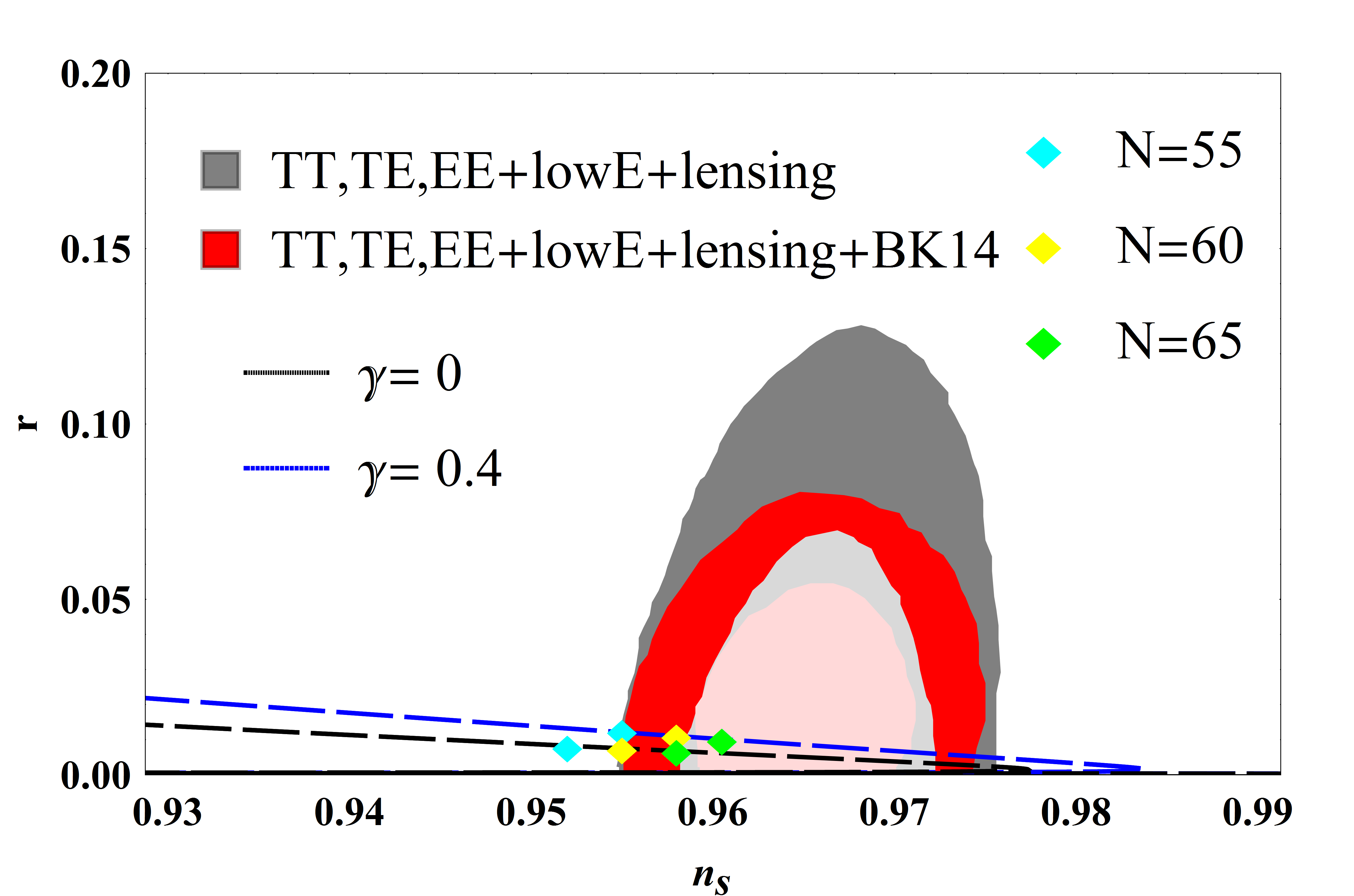
Finally, the ratio between the amplitude of tensor and scalar perturbations at the crossing horizon is given by
| (53) |
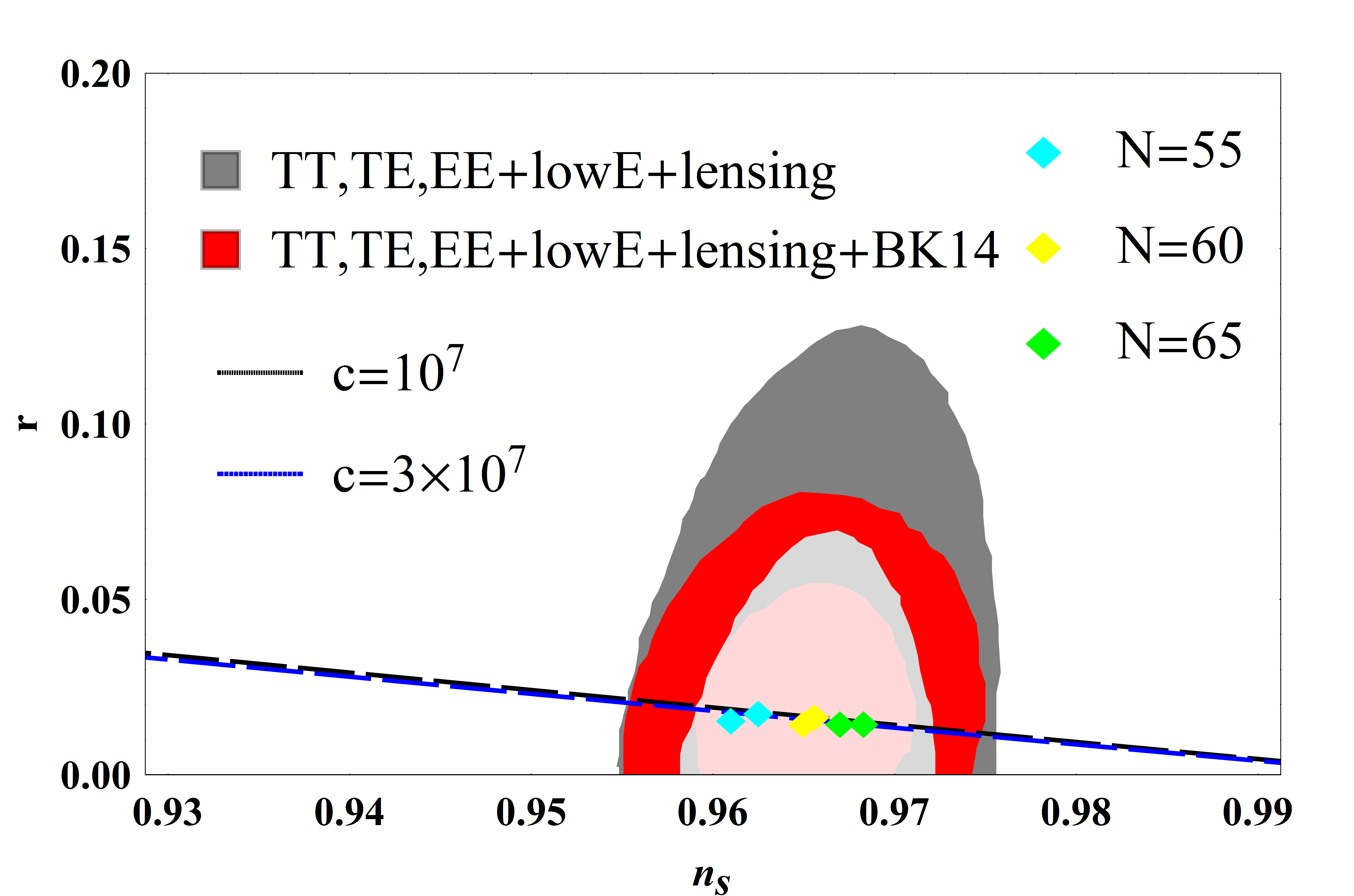
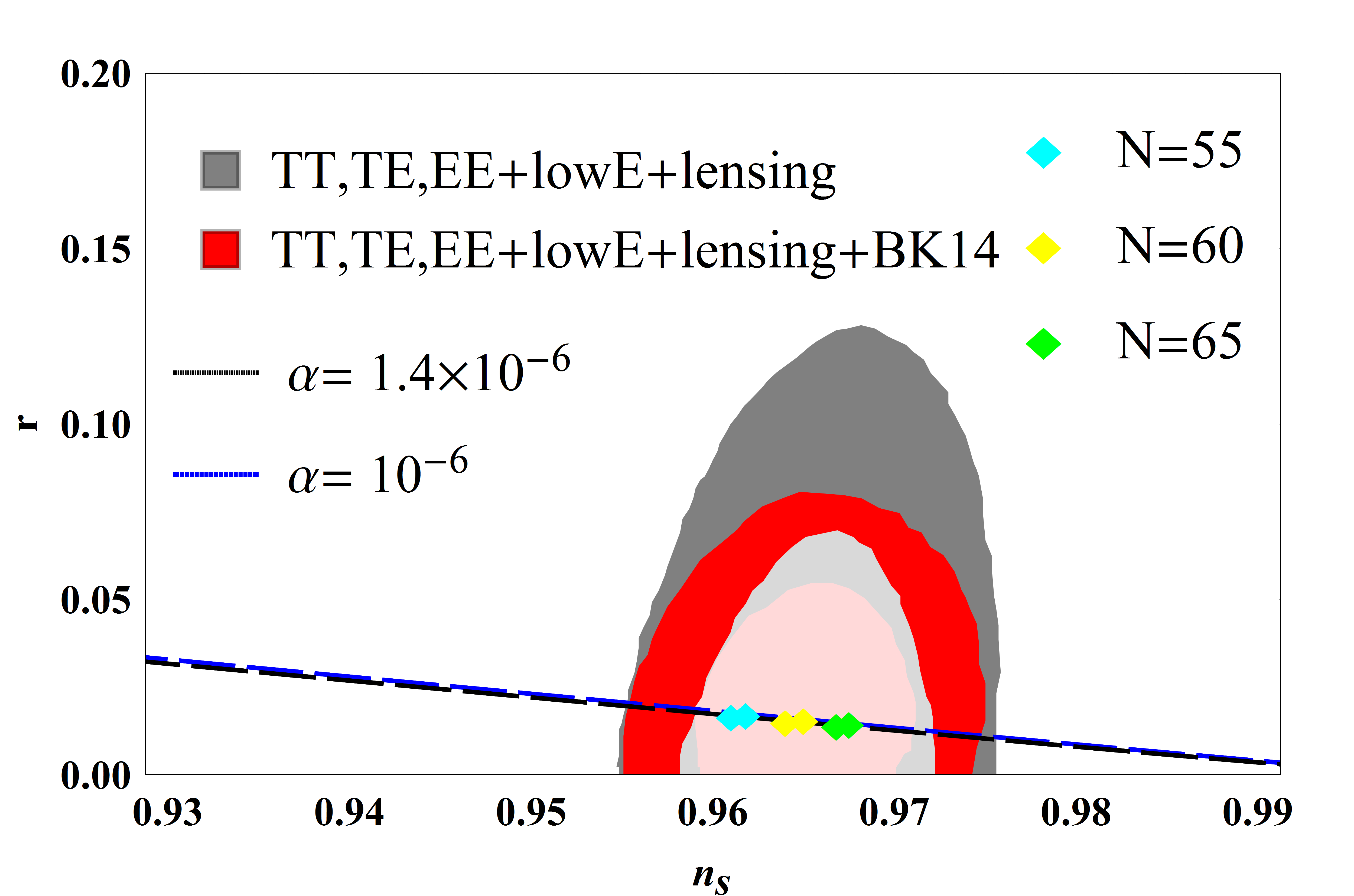
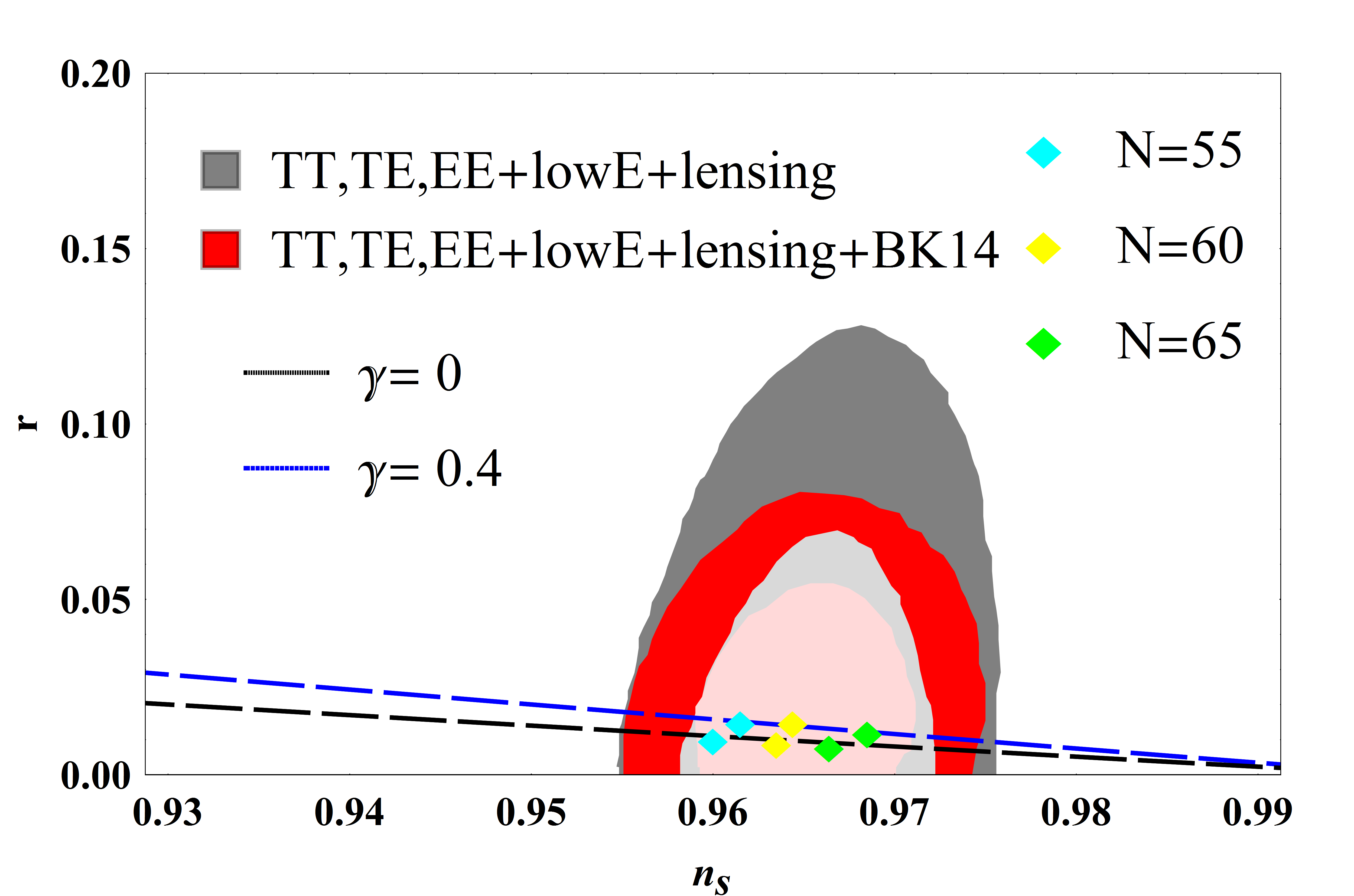
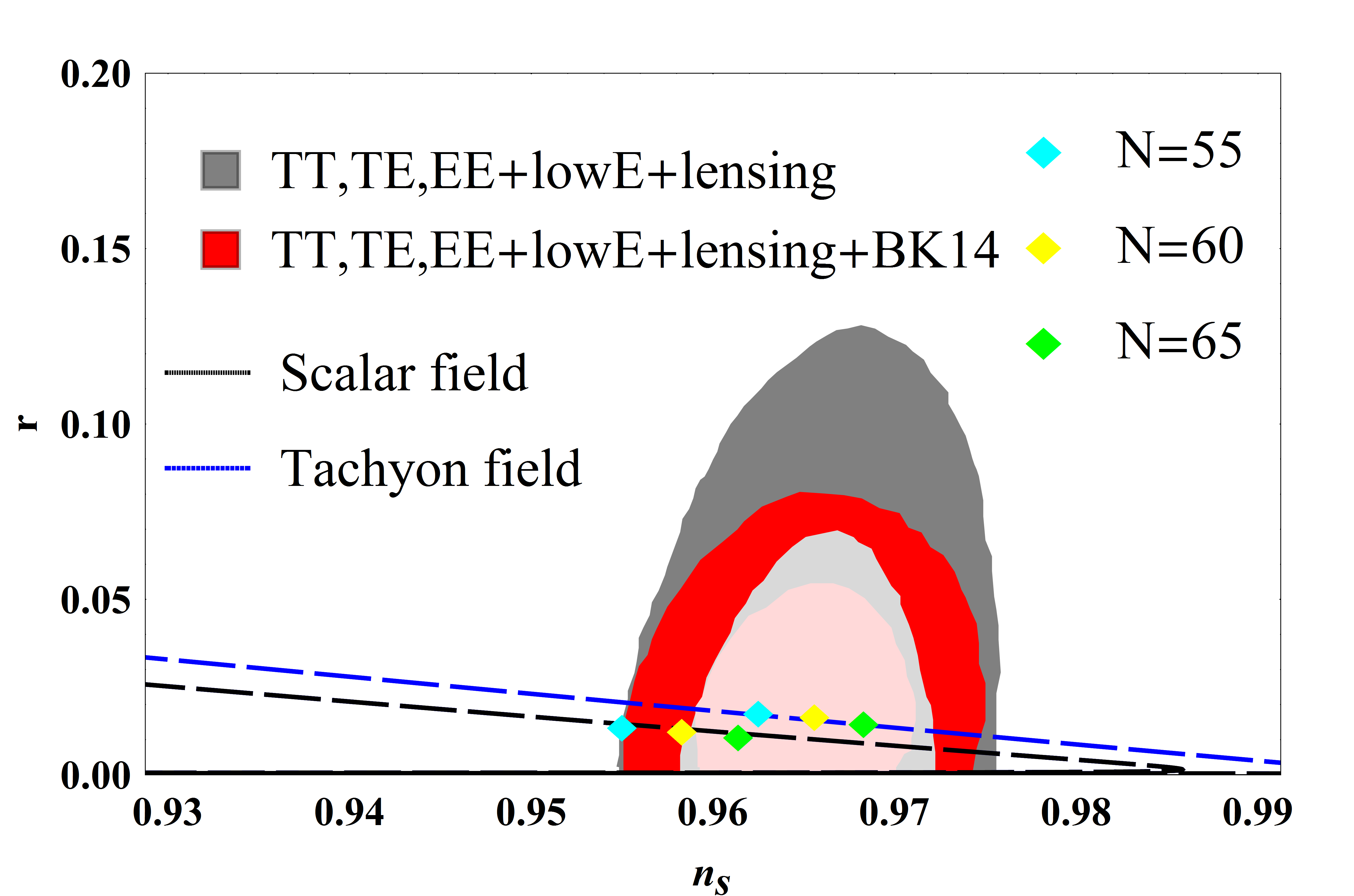
Figure 9 shows Constraints from the Planck TT, TE, EE+lowE+lensing data (gray contour) and Planck TT, TE, EE+lowE+lensing+BK14 data (red contour) in the plane. Figs. 9a, 9b and 9c are plotted for different values of , and respectively. The black and blue dashed lines represent theoretical predictions of the model parameters. We can see that our predicted parameters lie inside the 95% C. L. of the Planck data. In this figure we have highlighted three values of that are in the range . Furthermore, the value of the parameter used in these plots lies in the range estimated by authors in Ref. Bouabdallaoui:2016izz .
To compare the consistency between theoretical predictions and observations of the tachyon and the scalar fields, we plot the plane in Fig. 10. From this figure, one can notice a better agreement, at % C.L., for the tachyon than the scalar field for the selected numbers of e-folds. Furthermore, the scalar field shows smaller values of the tensor to scalar ratio compared to the tachyon field But both of them still fit the data quit well.
IV Summary and conclusions
In this paper, we have studied the cosmological inflation on a de Sitter brane with an induced gravity correction within the holographic cosmology. By considering a universe filled by both scalar and tachyon fields separately, we expressed the field equations in the slow-roll approximation. We have assumed a quadratic potential, for the scalar field, which has proven to be quite successful in constraining model’s parameters, then we have adopted an exponential potential for the tachyon field.
We have found that, the effect of the IG and the holographic cosmology is not negligible in the range of as can be seen from Fig. 1. We have also noted that the main perturbation parameters such as the scalar spectral index, its running and the tensor-to-scalar ratio are modified by some correction terms which are illustrated in Figs. 2 and 3. As these figures show, our results are affected by induced gravity corrections for in addition to the holographic cosmology for .
In order to check the consistency of the predicted parameters with observation, we have compared our results against those of Planck 2018 data by plotting the Planck confidence contours in the plane of . In this regard, the comparison indicates that the predicted parameters are consistent with the observational data, in the appropriate range of the conformal anomaly coefficient and the IG term, for both scalar and tachyon fields Figs. (6-9).
We have noticed a better agreement to the observational data, at % C.L., for the tachyon than the scalar field for the selected numbers of e-folds. Furthermore, while the scalar field shows smaller values of the tensor to scalar ratio compared to the tachyon field, both of the tachyon and the scalar fields are in good agreement with the Planck 2018 data. On the other hand, it can be also noted that the presence of the IG correction allows to expand the range of the conformal anomaly coefficient, see Eq.(40), compared to the range found by authors in Ref. Bouabdallaoui:2016izz .
Acknowledgment
The authors would like to thank Mariam Bouhmadi-López for many useful discussions and suggestions.
References
- (1) A. D. Linde, Contemp. Concepts Phys. 5 (1990) 1 [hep-th/0503203].
- (2) V. Mukhanov, Physical Foundations of Cosmology (Cambridge University Press, 2005).
- (3) V. F. Mukhanov, H. A. Feldman and R. H. Brandenberger, Phys. Rept. 215 (1992) 203.
- (4) C. L. Bennett et al., “Nine-Year Wilkinson Microwave Anisotropy Probe (WMAP) Observations: Final Maps and Results,” Astrophys. J. Suppl. (2013) 20; P. A. R. Ade et al., “Planck 2015 results. XX. Constraints on inflation,” (2015); P. Ade et al., “Joint Analysis of BICEP2/KeckArray and Planck Data,” Phys. Rev. Lett. (2015) 101301.
- (5) J. F. Donoghue, Phys. Rev. Lett. 72, (1994) 2996, [arXiv:gr-qc/9310024]. H. W. Hamber and S. Liu, Phys. Lett. B357, (1995) 51, [arXiv:hep-th/9505182]. N. H. Barth and S. M. Christensen, Phys. Rev. D28, (1983) 1876.
- (6) E. Kiritsis, JCAP 0510 (2005) 014 [hep-th/0504219].
- (7) J. de Boer, E. Verlinde, and H. Verlinde, JHEP 08 (2000) 003; E. Verlinde and H. Verlinde, JHEP. 05 (2000) 034; J. de Boer, Fortschr. Phys. 49 (2001) 339.
- (8) M. Bouhmadi-López and D. Wands, Phys. Rev. D 71 (2005) 024010 [hep-th/0408061].
- (9) J. E. Lidsey and D. Seery, Phys. Rev. D 73 (2006) 023516 [astro-ph/0511160].
- (10) G. R. Dvali and S. H. H. Tye, Phys. Lett. B 450 (1999) 72 [hep-ph/9812483].
- (11) C. Deffayet, Phys. Rev. D 66 (2002) 103504 [hep-th/0205084].
- (12) G. Kofinas, JHEP 0108 (2001) 034 [hep-th/0108013].
- (13) C. Deffayet, Phys. Lett. B 502 (2001) 199 [hep-th/0010186].
- (14) E. Kiritsis, N. Tetradis and T. N. Tomaras, JHEP 0203 (2002) 019 [hep-th/0202037].
- (15) L. Randall and R. Sundrum, Phys. Rev. Lett. 83 (1999) 4690 [hep-th/9906064].
- (16) J. M. Maldacena, Int. J. Theor. Phys. 38 (1999) 1113 [Adv. Theor. Math. Phys. 2 (1998) 231] [hep-th/9711200]; E. Witten, Adv. Theor. Math. Phys. 2 (1998) 253 [hep-th/9802150]; S. S. Gubser, I. R. Klebanov and A. M. Polyakov, Phys. Lett. B 428 (1998) 105 [hep-th/9802109].
- (17) O. Aharony, S. S. Gubser, J. M. Maldacena, H. Ooguri and Y. Oz, Phys. Rept. 323 (2000) 183 [hep-th/9905111].
- (18) Z. Bouabdallaoui, A. Errahmani, M. Bouhmadi-López and T. Ouali, Phys. Rev. D 94 (2016) 123508 [hep-th/1610.01963 ].
- (19) K. i. Maeda, S. Mizuno and T. Torii, Phys. Rev. D 68 (2003) 024033 [gr-qc/0303039].
- (20) E. Papantonopoulos and V. Zamarias, JCAP 0410 (2004) 001 [gr-qc/0403090].
- (21) M. Bouhmadi-López, R. Maartens and D. Wands, Phys. Rev. D 70 (2004) 123519 [hep-th/0407162].
- (22) M. Bouhmadi-López, Y. W. Liu, K. Izumi and P. Chen, Phys. Rev. D 89 (2014) no.6, 063501 [hep-th/1308.5765].
- (23) H. Collins and B. Holdom, Phys. Rev. D 62 (2000) 105009 [hep-ph/0003173].
- (24) G. R. Dvali, G. Gabadadze and M. Porrati, Phys. Lett. B 485 (2000) 208 [hep-th/0005016].
- (25) A. H. Guth, Phys. Rev. D 23 (1981) 347 [Adv. Ser. Astrophys. Cosmol. 3 (1987) 139].
- (26) G. Huey and J. E. Lidsey, Phys. Lett. B 514 (2001) 217 [astro-ph/0104006].
- (27) R. R. Caldwell, Phys. Lett. B 545 (2002) 23 [astro-ph/9908168].
- (28) E. J. Copeland, M. Sami and S. Tsujikawa, Int. J. Mod. Phys. D 15 (2006) 1753 [hep-th/0603057].
- (29) E. Papantonopoulos and Papa, Mod. Phys. Lett. A 15, (2000) 2145; Phys. Rev. D 63, (2000) 103506; S. H. S. Alexander, Phys. Rev. D 65, (2001) 023507; A. Mazumdar, S. Panda, A. Perez-Lorenzana, Nucl. Phys. B 614, (2001) 101; Shinji Mukohyama, Phys. Rev. D 66, (2002) 024009; M. Sami, Mod. Phys. Lett. A 18, (2003) 691.
- (30) H. Farajollahi, A. Ravanpak, Phys. Rev. D 84, (2011) 084017.
- (31) A. Sen, JHEP 0207 (2002) 065 [hep-th/0203265].
- (32) Y. S. Piao, R. G. Cai, X. m. Zhang and Y. Z. Zhang, Phys. Rev. D 66 (2002) 121301 [hep-ph/0207143].
- (33) V. Kamali and M. R. Setare, Adv. High Energy Phys. 2016 (2016) 9682398 [gr-qc/1508.05479].
- (34) R. Herrera, S. del Campo and C. Campuzano, JCAP 10 (2006) 009; M. R. Setare and V. Kamali, JCAP 034 (2012) 1208; A. Deshamukhya and S. Panda, Int. J. Mod. Phys. D 18 (2009) 2093; M. Bastero-Gil, A. Berera, N. Kronberg, [hep-ph/1509.07604].
- (35) J. Garriga and V. F. Mukhanov, Phys. Lett. B 458 (1999) 219.
- (36) Y. Akrami et al. [Planck Collaboration], [astro-ph.CO/1807.06211].
- (37) A. Bargach, F. Bargach and T. Ouali, Nucl. Phys. B 940 (2019) 10 [hep-th/1805.02942].
- (38) J. M. Bardeen, Phys. Rev. D 22 (1980) 1882.
- (39) V. F. Mukhanov, H. A. Feldman and R. H. Brandenberger, Phys. Rept. 215 (1992) 203.
- (40) R. Maartens, D. Wands, B. A. Bassett and I. Heard, Phys. Rev. D 62 (2000) 041301 [hep-ph/9912464].
- (41) K. Nozari and N. Rashidi, Phys. Rev. D 86 (2012) 043505 [gr-qc/1207.3966].
- (42) K. Nozari and N. Rashidi, Phys. Rev. D 88 (2013) no.2, 023519 [gr-qc/1306.5853].
- (43) C. Armendariz-Picon, T. Damour and V. F. Mukhanov, Phys. Lett. B 458 (1999) 209 [hep-th/9904075].
- (44) L. A. Urena-Lopez and M. J. Reyes-Ibarra, Int. J. Mod. Phys. D 18 (2009) 621 [astro-ph/0709.3996].
- (45) A.P.Billyard, The Asymptotic Behaviour of Cosmological Models Containing Matter and Scalar Fields (PhD thesis, Dalhousie University, 1999).
- (46) M. Sami, Pravabati Chingangbam, Tabish Qureshi, Phys. Rev. D 66 (2002) 043530.