Low-scale seesaw from neutrino condensation

Abstract

Knowledge of the mechanism of neutrino mass generation would help understand a lot more about Lepton Number Violation (LNV), the cosmological evolution of the Universe, or the evolution of astronomical objects. Here we propose a verifiable and viable extension of the Standard model for neutrino mass generation, with a low-scale seesaw mechanism via LNV condensation in the sector of sterile neutrinos. To prove the concept, we analyze a simplified model of just one single family of elementary particles and check it against a set of phenomenological constraints coming from electroweak symmetry breaking, neutrino masses, leptogenesis and dark matter. The model predicts (i) TeV scale quasi-degenerate heavy sterile neutrinos, suitable for leptogenesis with resonant enhancement of the $CP$ asymmetry, (ii) a set of additional heavy Higgs bosons whose existence can be challenged at the LHC, (iii) an additional light and sterile Higgs scalar which is a candidate for decaying warm dark matter, and (iv) a majoron. Since the model is based on simple and robust principles of dynamical mass generation, its parameters are very restricted, but remarkably it is still within current phenomenological limits.

I Introduction

The Lagrangian of the Standard model (SM) of elementary particles has an accidental $\mathrm{U}(1)_{L}$ symmetry of conservation of lepton number $L$. Nowadays there are at least three reasons why a sizable, beyond the SM, lepton number violation (LNV) should be considered. First, having a number of drawbacks such as the vacuum stability problem, lack of naturalness, or several hierarchy problems, the SM is increasingly understood as a low-energy effective model. As such, its renormalizable operators are just the leading-order terms in an infinite expansion of the effective Lagrangian, while the rest of the expansion consists of non-renormalizable operators of dimension larger than 4, which are suppressed by inverse powers of the scale of new physics. The least suppressed non-renormalizable operator, respecting all the SM local symmetries, is the dimension five Weinberg operator, which violates lepton number conservation by two units. Second, in order to explain naturally the smallness of neutrino masses, various seesaw mechanisms have been proposed, which rely on a LNV mixing of neutrino fields, giving rise to Majorana neutrino mass eigenstates. Third, LNV is a necessary condition for successful leptogenesis, which in turn could explain the baryon abundance of the Universe.

Usually these three aspects of LNV are jointly realized within extensions of the SM by seesaw mechanisms of various types, which provide neutrino masses naturally small compared to the charged fermion masses by means of a suppression coming from an inverse power of a large seesaw mass scale. The various types of seesaw mechanisms differ by the assumed origin of the seesaw mass scale as the mass of some new heavy fields, such as right-handed neutrinos, triplet scalar bosons, etc. Moreover, the size of the seesaw scale is not fixed purely by the size of the active neutrino masses, because other parameters may enter the neutrino mass formula. As such, the seesaw scale can have any value between the electroweak and Planck scales. Apart from theoretical restrictions in the form of postulating some symmetry or requiring some degree of naturalness, leptogenesis is what brings the most serious hints about the size of the seesaw scale, interpreted as a mass of heavy sterile Majorana neutrinos. This allows us to distinguish between high-scale and low-scale seesaw mechanisms. In fact, for successful leptogenesis, masses of the sterile neutrinos should be either very large, $10^{8}\mathrm{\,GeV}$ or more Davidson and Ibarra (2002), or if smaller, then they should be quasi-degenerate in order to resonantly enhance the $CP$ asymmetry Pilaftsis (1997), so defining the low-scale seesaw mechanism.

The low-scale seesaw mechanisms are attractive for their ability to offer an interesting phenomenology in the ballpark of current accelerator facilities. The extreme case, with quasi-degenerate sterile neutrinos of masses $\sim\mathcal{O}(10\mathrm{\,GeV})$, is the phenomenologically successful $\nu$MSM model, based on a type-I seesaw mechanism Asaka and Shaposhnikov (2005), which however requires tuning of a quite large number of free parameters, without any leading principle apart from phenomenological constraints. The linear and inverse seesaw mechanisms, on the other hand, contain heavy sterile Majorana neutrinos with quasi-degenerate masses in a more natural way, for the price of doubling the number of right-handed neutrino fields compared to the type-I seesaw mechanism. They also allow for setting up the seesaw scale to be lepton number conserving, which opens up the possibility of studying spontaneous LNV as a low-energy phenomenon. Motivated by these attractive features we elaborate our model on the basis of a combined inverse and linear low-scale seesaw mechanisms, where leptogenesis will provide the key ingredients to fix the model parameters.

The combined case of linear and inverse seesaw mechanisms is a natural consequence of the presence of two types of right-handed neutrinos Malinsky et al. (2005). Various models, implementing this scenario, have been proposed in the literature (for a recent review, see, for instance, Ref. Gavela et al. (2009)). Typically in these models the seesaw values of relevant parameters are set by hand, either directly as a new mass parameter or indirectly as a free parameter of a corresponding Yukawa coupling. In the present paper we propose a dynamical origin of the neutrino mass parameters rooted in neutrino condensation. The idea is that due to some new attractive force felt by neutrinos, LNV vacuum neutrino condensates are formed, and meson-like new (pseodo-)scalar bosons emerge as composite states of the neutrino fields. The seesaw mass matrix elements are generated dynamically as the vacuum expectation values (VEVs) of the composite scalars. Neutrino mass models with neutrino condensation and explicit LNV, has already been studied in the literature Martin (1991); Antusch et al. (2003); Smetana (2013a, b) in the context of type-I seesaw mechanism. Here we apply a similar strategy, in the framework of the linear and inverse seesaw mechanisms, assigning lepton number to right-handed neutrinos and selecting their LNV condensation channels in such a way that the new composite scalars also carry lepton number. The model Lagrangian is manifestly lepton number invariant and provides only lepton-number-conserving elements in the neutrino mass matrix. The lepton-number-violating elements, which trigger the combined linear and inverse seesaw mechanism, are dynamically generated, being proportional to VEVs of the composite scalars. Lepton number gets spontaneously broken and a massless composite majoron appears in the spectrum of the observable particles, along with a handful of other additional Higgs bosons.

In order to prove the phenomenological feasibility of our LNV neutrino condensation setup we parametrize the new neutrino-attracting force by a simple-minded four-neutrino interaction. Such an approximation allows for an analysis of the low-energy particle spectrum to a sufficient detail by standard tools of renormalizable effective Lagrangians Bardeen et al. (1990). Even though there might be many non-perturbative aspects of the neutrino condensation inaccessible within this approach, we believe that the main qualitative features and quantitative estimates can be reliably obtained. In what follows, we will show that, although the model has a rather limited parameter space, there is a phenomenologically acceptable parameter setting.

II Low-scale seesaw mechanisms and motivation of the Model

In this section we want to introduce the low-scale seesaw mechanism and motivate our model, which will be presented in detail in the next section.

The conventional seesaw mechanism of type I contains a neutrino Dirac mass $m_{D}$ coming from a Yukawa interaction with the Higgs field along with the electroweak symmetry breaking. In that case the seesaw scale is given by a right-handed Majorana neutrino mass $M_{R}$. Then the smallness of the neutrino mass relies on the suppression factor $m_{D}/M_{R}$. In contrast, the low-scale seesaw mechanism operates also with a small mass scale $\mu$, allowing for an additional suppression factor $\mu/m_{D}$, which relaxes the requirement on the seesaw scale $M_{R}$ to be extremely large, so that it may be not far above the reach of current high energy experiments.

The low-scale seesaw mechanism used in this work, limited here to a single generation, is built by introducing two right-handed neutrino fields, $\nu_{R},S_{R}$, which are sterile under the SM gauge group and by assuming a neutrino mass matrix of the form:

$$M_{\nu}=\left(\begin{array}[]{ccc}0&m_{D}&\mu_{\mathrm{lin}}\\ m_{D}&\mu^{\prime}_{\mathrm{inv}}&M_{R}\\ \mu_{\mathrm{lin}}&M_{R}&\mu_{\mathrm{inv}}\end{array}\right)\,$$ (1)

written in the basis $(\nu_{L},\ \nu^{c}_{R},\ S^{c}_{R})$. The $\nu_{L}-\nu_{L}^{c}$ element vanishes by the electroweak gauge symmetry. We shall set $\mu^{\prime}_{\mathrm{inv}}=0$ because, as it is argued in Appendix A, for our purposes it is not a phenomenologically significant parameter. By setting either $\mu_{\mathrm{inv/lin}}=0$ the linear/inverse seesaw scenarios are obtained, respectively.

To obtain one light $\nu$ and two heavy $N_{\pm}$ seesaw neutrino mass eigenstates, the following hierarchy is usually assumed:

$$\mu_{\mathrm{lin}},\mu_{\mathrm{inv}}\ll m_{D}\ll M_{R}\,.$$ (2)

One of the conclusions of our analysis is that we should end up with a slightly different hierarchy, namely:

$$\mu_{\mathrm{lin}}\ll\mu_{\mathrm{inv}}\sim m_{D}\ll M_{R}\,,$$ (3)

which however still provides a low-scale seesaw mechanism. By diagonalization of the neutrino mass matrix (1) with $\mu^{\prime}_{\mathrm{inv}}=0$, the light and heavy neutrino masses are obtained

$$m_{\nu} \simeq \mu_{\rm inv}\frac{m_{D}^{2}}{M_{R}^{2}}-2\mu_{\rm lin}\frac{m_{D}}{M_{R}}\,,$$ (4)

$$m_{N_{\pm}} \simeq M_{R}\pm\frac{1}{2}\mu_{\mathrm{inv}}$$ (5)

The lepton number assignment for the right-handed neutrino fields has a one-parameter freedom. There is a special assignment:

$$L(\nu_{r})=-L(S_{R})=1\,,$$ (6)

in which the mass $M_{R}$ is lepton number invariant. The only LNV mass parameters in (1) are $\mu_{\mathrm{lin}}$ and $\mu_{\mathrm{inv}}$ ($\mu^{\prime}_{\mathrm{inv}}$). If they are introduced via soft terms in the Lagrangian, then their values are protected by lepton number symmetry from acquiring large radiative corrections, i.e., their smallness is technically natural, and the necessary seesaw hierarchy (2) is preserved. Within our model, the LNV mass parameters appear dynamically, as they will be proportional to VEVs of composite scalar fields. Their smallness must result from the details of the underlying dynamics, which are, at this stage, not fully specified but just parametrized as four-fermion interactions.

III Model setup

We propose an extension of the SM with two sterile fermions $\nu_{R}$ and $S_{R}$, dubbed right-handed neutrinos, which form - with each other and with the SM leptons - composite scalar bosons via four-fermion interactions. In the present paper we limit ourselves to only one generation of fermions in order to develop the formalism and test the key phenomenological features of the model. The study of flavor physics in this framework is considered the next step, to be made elsewhere.

III.1 Effective theory description in terms of elementary fields

At the level of elementary fields, the Lagrangian in our model is given by

$$\mathcal{L} = \mathcal{L}_{\mathrm{SM}}^{\prime}+D^{\mu}H^{\dagger}D_{\mu}H-\mathcal{V}(H^{\dagger}H)-(y_{H}\overline{\ell_{L}}\tilde{H}\nu_{R}+\mathrm{h.c.})$$

$$+\mathrm{i}\bar{\nu}_{R}\partial/\nu_{R}+\mathrm{i}\bar{S}_{R}\partial/S_{R}-(\overline{S^{c}_{R}}M_{R}\nu_{R}+\mathrm{h.c.})$$

$$-G_{\mathrm{lin}}(\bar{\ell}_{L}S_{R})(\overline{S_{R}}\ell_{L})-G_{\mathrm{inv}}(\overline{S^{c}_{R}}S_{R})(\overline{S_{R}}S^{c}_{R})-G^{\prime}_{\mathrm{inv}}(\overline{\nu^{c}_{R}}\nu_{R})(\overline{\nu_{R}}\nu^{c}_{R})\,.$$

Here $\mathcal{L}_{\mathrm{SM}}^{\prime}$ is the single-family SM Lagrangian, from which we have pulled out the gauge-kinetic term of the Higgs field and the standard Higgs potential $\mathcal{V}(H^{\dagger}H)$, characterized by its parameters $\mu_{H}$ and $\lambda_{H}$.

The Lagrangian (III.1) is SM gauge-invariant and has a global lepton number symmetry $U(1)_{L}$, with the field assignment shown in Table 1.

Group	$\ell_{L}$	$H$	$\nu_{R}$	$S_{R}$	$\Sigma$	$\Phi$	$\Phi^{\prime}$
$\mathrm{U}(1)_{Y}$	$-1$	$+1$	$0$	$0$	$-1$	$0$	$0$
$\mathrm{U}(1)_{L}$	$+1$	$0$	$+1$	$-1$	$+2$	$-2$	$+2$
$\mathrm{SU}(2)_{L}$	$\mathbf{2}$	$\mathbf{2}$	$\mathbf{1}$	$\mathbf{1}$	$\mathbf{2}$	$\mathbf{1}$	$\mathbf{1}$

Table 1: The SM gauge group and lepton number assignments for the fields relevant for neutrino mass generation.

The global symmetries encounter the same axial anomalies as in the SM, generated by non-perturbative effects of the electroweak and QCD gauge dynamics. Therefore $B-L$ remains an exact symmetry.

We consider our model, defined by the Lagrangian $\mathcal{L}$ in Eq. (III.1), as an effective description of some more fundamental underlying theory at higher energy scales. Moreover, we assume that the field content of such an underlying theory can be divided into a heavy and a light sector, and for the characteristic scale of the heavy sector, $M_{\mathrm{heavy}}$, we assume $M_{\mathrm{heavy}}<\Lambda_{\mathrm{Planck}}$, in order to not reach quantum gravity effects. The light sector consists of the fields participating in the Lagrangian (III.1), which are all massless except for the elementary Higgs field with a $\mu_{H}$-mass parameter in the Higgs potential and the right-handed neutrino fields $\nu_{R}$, $S_{R}$ with their mass parameter $M_{R}$. The heavy sector of the underlying theory is integrated out and assumed to generate the four-neutrino interactions in Eq. (III.1), with the coupling constants of the order of

$$G_{\mathrm{lin}},G_{\mathrm{inv}},G_{\mathrm{inv}}^{\prime}\propto M_{\mathrm{heavy}}^{-2}\,.$$ (8)

Thus, $M_{\mathrm{heavy}}$ is a cut-off scale of the effective theory defined by the Lagrangian (III.1).

III.2 Condensation and energy scales

The key point of our model, based on Lagrangian (III.1), is the assumption that due to the attractiveness of the four-fermion interactions, the following scalar bound states of fermion pairs are formed:

$$\Sigma \sim (\overline{S_{R}}\ell_{L})\,,$$ (9a)

$$\Phi \sim (\overline{S^{c}_{R}}S_{R})\,,$$ (9b)

$$\Phi^{\prime} \sim (\overline{\nu^{c}_{R}}\nu_{R})\,,$$ (9c)

at some scale $\Lambda<M_{\mathrm{heavy}}$. At this same scale $\Lambda$ or somewhere below the composite bound states develop non-trivial VEVs, corresponding to the fermion-pair condensates

$$\langle\Sigma\rangle \equiv \frac{1}{\sqrt{2}}\left(\begin{array}[]{c}v_{\Sigma}\\ 0\end{array}\right)\sim\langle\overline{S_{R}}\ell_{L}\rangle\,,$$ (10c)

$$\langle\Phi\rangle \equiv \ \ \frac{v_{\Phi}}{\sqrt{2}}\quad\sim\ \langle\overline{S^{c}_{R}}S_{R}\rangle\,,$$ (10d)

$$\langle\Phi^{\prime}\rangle \equiv \ \ \frac{v_{\Phi^{\prime}}}{\sqrt{2}}\quad\sim\ \langle\overline{\nu^{c}_{R}}\nu_{R}\rangle\,.$$ (10e)

In what follows we shall call $\Lambda$ the compositeness scale. The VEVs $v_{\Sigma}$, $v_{\Phi}$ and $v_{\Phi}^{\prime}$ break $U(1)_{L}$, generating the $\Delta L=2$ entries of the mass matrix (1) of the neutrino sector, so that

$$\mu_{\mathrm{lin}} = \frac{y_{\Sigma}v_{\Sigma}}{\sqrt{2}}\,,$$ (11)

$$\mu_{\mathrm{inv}} = \frac{y_{\Phi}v_{\Phi}}{\sqrt{2}}\,,$$ (12)

$$\mu^{\prime}_{\mathrm{inv}} = \frac{y_{\Phi^{\prime}}v_{\Phi^{\prime}}}{\sqrt{2}}\,.$$ (13)

The effective Yukawa couplings $y_{\Sigma},y_{\Phi}$ and $y_{\Phi^{\prime}}$ stem from the four-fermion couplings $G_{\rm lin},G_{\rm inv}$ and $G^{\prime}_{\rm inv}$ in Eq. (III.1), and the corresponding relations between these Yukawas and four-fermion couplings will be discussed in the next sections.

The Dirac type entry is as usual

$$m_{D}=\frac{y_{H}v_{H}}{\sqrt{2}}\,,$$ (14)

where $v_{H}$ is the VEV developed by the elementary electroweak doublet Higgs field

$$\langle H\rangle=\frac{1}{\sqrt{2}}\left(\begin{array}[]{c}0\\ v_{H}\end{array}\right)\,,$$ (17)

according to its potential, which at tree level is not affected by the right-handed neutrino condensation and is governed mainly by the usual SM parameters $\mu_{H}$ and $\lambda_{H}$.

For our model it is crucial that the right-handed neutrinos are not too heavy to be integrated out before their condensation happens. Therefore we require the non-decoupling condition:

$$M_{R}<\Lambda\,.$$ (18)

For simplicity we will consider $\mu^{\prime}_{\mathrm{inv}}=0$ in the rest of this work, which can be interpreted as the fact that the corresponding four-fermion coupling constant $G^{\prime}_{\rm inv}$ is sub-critical so that $v_{\Phi}^{\prime}=0$. Moreover, we will take the even stronger assumption that $G^{\prime}_{\rm inv}$ is so weak that not even the bound state $\Phi^{\prime}$ is formed.

IV Effective description of the neutrino condensation

Here we use the formalism developed in Refs. Bardeen et al. (1990); Hill et al. (1991), which is suitable for the realization of the above-described scenario of neutrino condensation, starting from the attractive four-fermion interactions in the Lagrangian (III.1) of our model. Akin to the famous case of condensed matter physics, where the electron-pair condensation is preceded by Cooper-pairing, in our model the fermion-antifermion condensation inevitably involves formation of bound states, which in an effective theory are described by the corresponding effective bosonic fields, which in turn introduce new phenomenology at low energies. We start with the definition of this effective bosonized theory.

IV.1 Bosonization

As we already discussed, the key hypothesis of our model is that the attractive four-fermion interactions in Eq. (III.1) lead to the formation of bound states at the compositeness scale $\Lambda$, according to Eq. (9). This non-perturbative phenomenon can be suitably described by the bosonization prescription introducing the auxiliary fields $\Sigma_{\Lambda}$ and $\Phi_{\Lambda}$:

$$\mathcal{L}_{\mathrm{lin};\Lambda} = -(y_{\Sigma;\Lambda}\bar{\ell}_{L}\Sigma_{\Lambda}S_{R}+\mathrm{h.c.})-\mu^{2}_{\Sigma;\Lambda}\Sigma_{\Lambda}^{\dagger}\Sigma_{\Lambda}\,,$$ (19)

$$\mathcal{L}_{\mathrm{inv};\Lambda} = -(y_{\Phi;\Lambda}\overline{S_{R}}\Phi_{\Lambda}S^{c}_{R}+\mathrm{h.c.})-\mu^{2}_{\Phi;\Lambda}\Phi_{\Lambda}^{\dagger}\Phi_{\Lambda}\,.$$ (20)

The auxiliary fields have no kinetic terms and as such can be eliminated from the Lagrangian by means of their non-dynamical equations of motion

$$\Sigma_{\Lambda}^{\dagger} = \frac{y_{\Sigma;\Lambda}}{\mu^{2}_{\Sigma;\Lambda}}\bar{\ell}_{L}S_{R}\,,$$ (21)

$$\Phi_{\Lambda}^{\dagger} = \frac{y_{\Phi;\Lambda}}{\mu^{2}_{\Phi;\Lambda}}\overline{S_{R}}S^{c}_{R}\,,$$ (22)

and their respective hermitian conjugates for $\Sigma_{\Lambda}$ and $\Phi_{\Lambda}$. We thus recover the original four-fermion interactions from Eq. (III.1) by identifying the coefficients:

$$G_{\mathrm{lin}} = \frac{y_{\Sigma;\Lambda}^{2}}{\mu^{2}_{\Sigma;\Lambda}}\,,$$ (23a)

$$G_{\mathrm{inv}} = \frac{y_{\Phi;\Lambda}^{2}}{\mu^{2}_{\Phi;\Lambda}}\,.$$ (23b)

IV.2 Effective low-energy Lagrangian

The bosonized model Lagrangians (19) and (20) evolve from the scale $\Lambda$ down to some low-energy scale $m$, in accordance with the corresponding Renormalization Group Equations (RGEs),

$$\mathcal{L}_{\Lambda}\rightarrow\mathcal{L}_{m}\,.$$ (24)

As it is well known, the RGE evolution can be interpreted as integrating out the higher-energy field modes in the interval $(m,\Lambda)$. This procedure leads to the appearance of effective operators generated by quantum corrections, such as the kinetic terms of the composite fields $\Phi$ and $\Sigma$, which are weighed by the wave function renormalization coefficients $Z_{\Sigma,\Phi;m}$, whose main radiative one-loop contribution comes from the Yukawa interaction

$$Z_{\Sigma,\Phi;m}=\frac{y_{\Sigma,\Phi;\Lambda}^{2}}{(4\pi)^{2}}\ln\frac{\Lambda}{m}\ \sim\ \mathcal{O}(1)\ \stackrel{{\scriptstyle m\rightarrow\Lambda}}{{\longrightarrow}}\ 0\,.$$ (25)

The coefficients $Z_{\Sigma,\Phi;m}$ vanish in the limit $m\rightarrow\Lambda$, since the kinetic operators are not present in the Lagrangian (19) and (20), relevant for the scale $\Lambda$. On the other hand, the mass term operators are present at the scale $\Lambda$, and for $m<\Lambda$ their coefficients $\mu^{2}_{\Sigma,\Phi;m}$ only get radiative corrections from the Yukawa interaction according to

$$\mu^{2}_{\Sigma,\Phi;m}=\mu^{2}_{\Sigma,\Phi;\Lambda}-\frac{2y_{\Sigma,\Phi;\Lambda}^{2}}{(4\pi)^{2}}(\Lambda^{2}-m^{2})\ \stackrel{{\scriptstyle m\rightarrow\Lambda}}{{\longrightarrow}}\ \mu^{2}_{\Sigma,\Phi;\Lambda}\,.$$ (26)

Actually, it is not necessary to perform the above-mentioned integrating-out of the high-energy modes explicitly: it is sufficient to realize that all the operators allowed by the symmetries of the initial Lagrangian (19), (20) will be radiatively generated and contribute to the effective Lagrangian. Taking into account only the relevant operators, we end up after the necessary field normalization, with a renormalizable effective theory valid at scales lower than $\Lambda$, described by the effective Lagrangian

$$\mathcal{L}_{\mathrm{eff}} = \mathcal{L}_{\mathrm{SM}}^{\prime}+D^{\mu}H^{\dagger}D_{\mu}H+D^{\mu}\Sigma^{\dagger}D_{\mu}\Sigma+\partial^{\mu}\Phi^{\dagger}\partial_{\mu}\Phi-\mathcal{V}_{\mathrm{eff}}(H,\Sigma,\Phi)$$

$$-(y_{H}\overline{\ell_{L}}\tilde{H}\nu_{R}+y_{\Sigma}\bar{\ell}_{L}\Sigma S_{R}+y_{\Phi}\overline{S_{R}}\Phi S^{c}_{R}+\mathrm{h.c.})$$

$$+\mathrm{i}\bar{\nu}_{R}\partial/\nu_{R}+\mathrm{i}\bar{S}_{R}\partial/S_{R}-(\overline{S^{c}_{R}}M_{R}\nu_{R}+\mathrm{h.c.})\,,$$

where

$$\mathcal{V}_{\mathrm{eff}}(H,\Sigma,\Phi) = \mu_{H}^{2}H^{\dagger}H+\mu_{\Sigma}^{2}\Sigma^{\dagger}\Sigma+\mu_{\Phi}^{2}\Phi^{\dagger}\Phi$$

$$+\frac{1}{2}\lambda_{H}(H^{\dagger}H)^{2}+\frac{1}{2}\lambda_{\Sigma}(\Sigma^{\dagger}\Sigma)^{2}+\frac{1}{2}\lambda_{\Phi}(\Phi^{\dagger}\Phi)^{2}$$

$$+\lambda_{\Phi H}(\Phi^{\dagger}\Phi)(H^{\dagger}H)+\lambda_{\Phi\Sigma}(\Phi^{\dagger}\Phi)(\Sigma^{\dagger}\Sigma)$$

$$+\lambda_{H\Sigma}(H^{\dagger}H)(\Sigma^{\dagger}\Sigma)+\lambda^{\prime}_{H\Sigma}(\Sigma^{\dagger}\tilde{H})(\tilde{H}^{\dagger}\Sigma)$$

$$+\Big{[}\kappa\,\Phi^{\dagger}(H^{\dagger}\tilde{\Sigma})+\mathrm{h.c.}\Big{]},$$

is the effective potential for the scalar fields.

The parameters of the effective Lagrangian run according to their RGEs. We use one-loop RGEs given in Appendix C and proceed with the standard strategy given, e.g., in Hill et al. (1991); Cvetic (1999); Antusch et al. (2003). The parameters $y_{\Sigma}$, $y_{\Phi}$, $\lambda_{\Sigma}$, $\lambda_{\Phi}$, $\lambda_{H\Sigma}$, $\lambda^{\prime}_{H\Sigma}$, $\lambda_{\Phi H}$, $\lambda_{\Phi\Sigma}$ and $\kappa$ are dynamically generated by their RGE running from specific boundary conditions, which follow from the matching of the Lagrangians $\mathcal{L}_{m}$ [Eq. (24)] and $\mathcal{L}_{\mathrm{eff}}$ [Eq. (IV.2)] at the compositeness scale $\Lambda$, and from the renormalization of the $\mathcal{L}_{m}$ parameters $Z_{\Sigma;m}$, $Z_{\Phi;m}$, $y_{\Sigma;m}$, $y_{\Phi;m}$, $\lambda_{\Sigma;m}$, $\lambda_{\Phi;m}$, $\lambda_{H\Sigma;m}$, $\lambda^{\prime}_{H\Sigma;m}$, $\lambda_{\Phi H;m}$, $\lambda_{\Phi\Sigma;m}$ and $\kappa_{m}$ shown, e.g., in Eq. (25). From the relation between the Lagrangians $\mathcal{L}_{m}$ and $\mathcal{L}_{\mathrm{eff}}$, which is given by the proper normalization of the kinetic terms of the composite scalar fields

$$\mathcal{L}_{\mathrm{eff}}(\Sigma,\Phi)=\mathcal{L}_{m}(\Sigma_{m}\rightarrow\Sigma/\sqrt{Z_{\Sigma;m}}\,,\,\Phi_{m}\rightarrow\Phi/\sqrt{Z_{\Phi;m}}),$$ (29)

we obtain the relations

$$\mu_{\Sigma}^{2}=\frac{\mu_{\Sigma;m}^{2}}{Z_{\Sigma;m}}\,,\,\mu_{\Phi}^{2}=\frac{\mu_{\Phi;m}^{2}}{Z_{\Phi;m}}\,,$$ (30)

$$y_{\Sigma}=\frac{y_{\Sigma;m}}{\sqrt{Z_{\Sigma;m}}}\,,\,y_{\Phi}=\frac{y_{\Phi;m}}{\sqrt{Z_{\Phi;m}}}\,,\kappa=\frac{\kappa_{m}}{\sqrt{Z_{\Sigma;m}Z_{\Phi;m}}}\,,$$ (31)

$$\lambda_{\Sigma}=\frac{\lambda_{\Sigma;m}}{Z_{\Sigma;m}^{2}}\,,\,\lambda_{\Phi}=\frac{\lambda_{\Phi;m}}{Z_{\Phi;m}^{2}}\,,\,\lambda_{H\Sigma}=\frac{\lambda_{H\Sigma;m}}{Z_{\Sigma;m}}\,,\,$$ (32)

$$\lambda^{\prime}_{H\Sigma}=\frac{\lambda^{\prime}_{H\Sigma;m}}{Z_{\Sigma;m}}\,,\,\lambda_{\Phi H}=\frac{\lambda_{\Phi H;m}}{Z_{\Phi;m}}\,,\,\lambda_{\Phi\Sigma}=\frac{\lambda_{\Phi\Sigma;m}}{Z_{\Sigma;m}Z_{\Phi;m}}\,.$$ (33)

From these relations we get the boundary conditions at the matching scale $\Lambda$

$$y_{\Sigma}\,,\,y_{\Phi} \stackrel{{\scriptstyle m\rightarrow\Lambda}}{{\longrightarrow}} \infty\,,$$ (34)

$$\frac{\lambda_{\Sigma}}{y_{\Sigma}^{4}}\,,\,\frac{\lambda_{\Phi}}{y_{\Phi}^{4}}\,,\,\frac{\lambda_{H\Sigma}}{y_{\Sigma}^{2}}\,,\,\frac{\lambda^{\prime}_{H\Sigma}}{y_{\Sigma}^{2}}\,,\,\frac{\lambda_{\Phi H}}{y_{\Phi}^{2}}\,,\,\frac{\lambda_{\Phi\Sigma}}{y_{\Sigma}^{2}y_{\Phi}^{2}} \stackrel{{\scriptstyle m\rightarrow\Lambda}}{{\longrightarrow}} 0\,,$$ (35)

$$\frac{\kappa}{y_{\Sigma}y_{\Phi}} \stackrel{{\scriptstyle m\rightarrow\Lambda}}{{\longrightarrow}} 0\,.$$ (36)

Notice that the boundary conditions for the Yukawa parameters (34) exhibit an ill behavior. When approaching the matching scale $\Lambda$ from below, these Yukawa parameters grow, indicating their non-perturbative origin. In fact, these couplings appear as a result of the formation of the bound states $\Sigma$ and $\Phi$ at the scale $\Lambda$, which is essentially a non-perturbative phenomenon. Therefore, once $y_{\Sigma}\,,\,y_{\Phi}$ become larger than some value – typically $4\pi$ – the perturbative one-loop RGEs cannot be trusted anymore. In practice this means that we have lost the relation between $y_{\Sigma}\,,\,y_{\Phi}$ of the effective theory (IV.2) and the four-fermion couplings in Eqs. (23) of the underlying theory (III.1). Consequently, instead of using the ill defined matching condition we follow the standard strategy described in e.g. Hill et al. (1991); Cvetic (1999); Antusch et al. (2003), and for ease of numerical calculations we set

$$y_{\Sigma}(\Lambda)=y_{\Phi}(\Lambda)=y_{0}\,,$$ (37)

where $y_{0}$ is some finite value, typically $\sim 4\pi$. As will be shown below, such arbitrariness in the boundary condition is justified by the fact that the low-energy values are only very weakly sensitive to the high-energy values of $y_{\Sigma}\,,\,y_{\Phi}$.

From (35), (36) and (37) we obtain the boundary conditions for the rest of the parameters:

$$\lambda_{K}(\Lambda) = 0\,,\ \ K=\Sigma,\Phi,H\Sigma,H\Sigma^{\prime},\Phi H,\Phi\Sigma\,,$$ (38)

$$\kappa(\Lambda) = 0\,.$$ (39)

The effective scalar potential $\mathcal{V}_{\mathrm{eff}}(H,\Sigma,\Phi)$ in Eq. (IV.2) has a non-trivial minimum, which defines the symmetry breaking pattern. As in the SM, we assume $\mu_{H}^{2}<0$. In order that both LNV VEVs, $v_{\Sigma}$ and $v_{\Phi}$, have nonzero values, $\mu_{\Sigma}^{2}$ and $\mu_{\Phi}^{2}$ must be negative.

Now, in order to set up a low-scale seesaw mechanism, both $\mu_{\mathrm{lin}}$ and $\mu_{\mathrm{inv}}$ have to be small compared to the other neutrino mass parameters. Since the Yukawa coupling parameters in (11) and (12) do not help guaranteeing this smallness, because $y_{\Sigma,\Phi}\sim 1$, the VEVs $v_{\Sigma}$ and $v_{\Phi}$ must be small, which requires the smallness of $|\mu_{\Sigma}^{2}|$ and $|\mu_{\Phi}^{2}|$ at low scales $m\rightarrow 0$. Accordingly, Eqs. (23) and (26) provide a requirement on the underlying four-fermion interaction parameters $G_{\mathrm{lin}}$ and $G_{\mathrm{inv}}$, which have to be tuned to be just slightly super-critical:

$$\mathrm{to\ obtain}\ \ |\mu_{\Sigma,\Phi}^{2}|\ll\Lambda^{2}\ :\ \ \ 0<\frac{G_{\mathrm{lin},\mathrm{inv}}}{G_{\mathrm{lin},\mathrm{inv}}^{\mathrm{crit}}}-1\ll 1$$ (40)

where $G_{\mathrm{lin},\mathrm{inv}}^{\mathrm{crit}}\equiv 8\pi^{2}/\Lambda^{2}$ is the critical value of the four-fermion coupling parameters. We do not try to explain this feature of the underlying new dynamics in this work, but keep it as one of the subjects for future work.

Interestingly, our model allows for a unique triple scalar coupling in Eq. (IV.2) with the calculable constant $\kappa$. As will be shown in what follows, this triple coupling plays an essential role in order to meet all the phenomenological constraints. Although the coupling constant $\kappa$ is in general complex, its phase can be absorbed into the redefinition of the field $\Phi$. Therefore, all the coupling constants in the effective potential are real parameters. This phase absorption corresponds to the known fact that in the scalar sector of a model with two Higgs doublets and one complex Higgs singlet, there is no source of CP violation Ivanov (2017).

IV.3 Generalized Weinberg operators

The right-handed neutrino mass $M_{R}$ is the highest mass scale in our model, and below this scale the right-handed neutrinos decouple from the low-energy observables. As a consequence, below $M_{R}$ all three neutrino Yukawa interactions weighed by the Yukawa coupling parameters $y_{H}$, $y_{\Sigma}$ and $y_{\Phi}$, are traded for the effective operators of higher dimensions that result from integrating out the right-handed neutrinos. The part of the Lagrangian containing these effective operators is

$$\mathcal{L}_{w}=\frac{w_{\mathrm{inv}}}{2M_{R}^{2}}(\bar{\ell}_{L}\tilde{H})\Phi(H^{\dagger}\ell_{L}^{c})+\frac{w_{\mathrm{lin}}}{M_{R}}(\bar{\ell}_{L}\Sigma)(H^{\dagger}\ell_{L}^{c})+\mathrm{h.c.}$$ (41)

We will refer to these operators as generalized Weinberg operators, where $w_{\mathrm{inv}}$ and $w_{\mathrm{lin}}$ are dimensionless Weinberg parameters. After the scalar fields develop their VEVs, these terms will directly provide the Majorana mass term for the active neutrino

$$\mathcal{L}_{m_{\nu}}=\frac{1}{2}m_{\nu}(\bar{\nu}_{L}\nu_{L}^{c})+\mathrm{h.c.}\,,$$ (42)

where $m_{\nu}$ is obtained from $\mathcal{L}_{w}$ in Eq. (41) as:

$$m_{\nu}=w_{\mathrm{inv}}\frac{v_{H}^{2}v_{\Phi}}{2\sqrt{2}M_{R}^{2}}+w_{\mathrm{lin}}\frac{v_{H}v_{\Sigma}}{2M_{R}}\,.$$ (43)

On the other hand, calculating the same $m_{\nu}$ from $\mathcal{L}_{\mathrm{eff}}$ in Eq. (IV.2), we obtain an expression for the neutrino mass in terms of the Yukawa couplings:

$$m_{\nu}=y_{H}^{2}y_{\Phi}\frac{v_{H}^{2}v_{\Phi}}{2\sqrt{2}M_{R}^{2}}-y_{H}y_{\Sigma}\frac{v_{H}v_{\Sigma}}{M_{R}}\,.$$ (44)

This leads to the matching condition at the scale $M_{R}$

$$\left.w_{\mathrm{inv}}\right|_{m=M_{R}} = \left.y_{H}^{2}y_{\Phi}\right|_{m=M_{R}}\,,$$ (45)

$$\left.w_{\mathrm{lin}}\right|_{m=M_{R}} = \left.-2y_{H}y_{\Sigma}\right|_{m=M_{R}}\,.$$ (46)

Introducing the generalized Weinberg operators has the advantage of allowing us to avoid the procedure of diagonalizing the neutrino mass matrix (1) in order to determine the light neutrino mass, which would require inserting the low-energy values of the Yukawa coupling parameters $y_{H,\Sigma,\Phi}(m_{\mathrm{low}})$ into the entries of the neutrino mass matrix (1). In principle, the low-energy scale, at which the neutrino mass is determined, $m_{\mathrm{low}}$, should be taken of the same order of magnitude as the neutrino mass itself $m_{\mathrm{low}}\sim m_{\nu}$. This would, however, entale a trouble, because the one-loop RGEs drive the Yukawa couplings to large non-perturbative values at such small energy scale. This problem is eliminated by trading, at the $M_{R}$-scale, the Yukawa couplings for the Weinberg parameters, whose RGE running is safe all the way down to arbitrarily low scales.

IV.4 Minimization of the effective potential and symmetry breaking

The minimum of the effective potential $\mathcal{V}_{\mathrm{eff}}(H,\Sigma,\Phi)$ in Eq. (IV.2) determines the values of the VEVs (10) and (17) as a solution of the equations

$$\frac{\partial}{\partial v_{H}}\mathcal{V}_{\mathrm{eff}}(\langle H\rangle,\langle\Sigma\rangle,\langle\Phi\rangle) = 0\,,$$ (47)

$$\frac{\partial}{\partial v_{\Sigma}}\mathcal{V}_{\mathrm{eff}}(\langle H\rangle,\langle\Sigma\rangle,\langle\Phi\rangle) = 0\,,$$ (48)

$$\frac{\partial}{\partial v_{\Phi}}\mathcal{V}_{\mathrm{eff}}(\langle H\rangle,\langle\Sigma\rangle,\langle\Phi\rangle) = 0\,.$$ (49)

Explicitly we have

$$-\mu_{H}^{2} = \frac{1}{2v_{H}}\Big{[}-\sqrt{2}\kappa v_{\Sigma}v_{\Phi}+\lambda_{H}v_{H}^{3}+(\lambda_{H\Sigma}+\lambda^{\prime}_{H\Sigma})v_{H}v_{\Sigma}^{2}+\lambda_{\Phi H}v_{H}v_{\Phi}^{2}\Big{]}\,,$$

$$-\mu_{\Sigma}^{2} = \frac{1}{2v_{\Sigma}}\Big{[}-\sqrt{2}\kappa v_{H}v_{\Phi}+\lambda_{\Sigma}v_{\Sigma}^{3}+(\lambda_{H\Sigma}+\lambda^{\prime}_{H\Sigma})v_{\Sigma}v_{H}^{2}+\lambda_{\Phi\Sigma}v_{\Sigma}v_{\Phi}^{2}\Big{]}\,,$$

$$-\mu_{\Phi}^{2} = \frac{1}{2v_{\Phi}}\Big{[}-\sqrt{2}\kappa v_{H}v_{\Sigma}+\lambda_{\Phi}v_{\Phi}^{3}+\lambda_{\Phi H}v_{H}^{2}v_{\Phi}+\lambda_{\Phi\Sigma}v_{\Sigma}^{2}v_{\Phi}\Big{]}$$ (50)

in accordance with Ref. Chalons and Domingo (2012). These equations can be used to trade the $\mu_{H,\Sigma,\Phi}$ parameters for the VEVs $v_{\Sigma}$, $v_{\Phi}$ and $v_{H}$ in the potential $\mathcal{V}_{\mathrm{eff}}(H,\Sigma,\Phi)$ of Eq. (IV.2). From Eqs. (50) we can see that unless $\kappa=0$, the solution with all three VEVs $v_{H}$, $v_{\Sigma}$ and $v_{\Phi}$ non-zero is the only one available.

The stability of the vacuum is guaranteed by the positive definiteness of the Hessian matrix

$$\mathcal{H}_{ij}\equiv\frac{\partial^{2}}{\partial v_{i}\partial v_{j}}\mathcal{V}_{\mathrm{eff}}(\langle H\rangle,\langle\Sigma\rangle,\langle\Phi\rangle) \ \ \mathrm{where}\ \ \ i,j=H,\Sigma,\Phi\,,$$ (51)

which is calculated by using Eqs. (50) and is actually equivalent to the scalar boson mass matrix, written explicitly in Eq. (177).

V Properties of Higgs bosons

In order to derive the properties of the physical Higgs scalar excitations, we shift their fields by their VEVs:

$$H = \left(\begin{array}[]{c}a_{H}^{+}\\ (v_{H}+h_{H}+\mathrm{i}a_{H})/\sqrt{2}\end{array}\right)\,,$$ (52c)

$$\Sigma = \left(\begin{array}[]{c}(v_{\Sigma}+h_{\Sigma}+\mathrm{i}a_{\Sigma})/\sqrt{2}\\ a_{\Sigma}^{-}\end{array}\right)\,,$$ (52f)

$$\Phi = (v_{\Phi}+h_{\Phi}+\mathrm{i}a_{\Phi})/\sqrt{2}\,,$$ (52g)

by which the effective potential (IV.2) becomes a function of the fields corresponding to the true ground state:

$$\mathcal{V}_{\mathrm{eff}}(H,\Sigma,\Phi)\longrightarrow\mathcal{V}_{\mathrm{eff}}(\vec{\phi})\,,$$ (53)

where

$$\vec{\phi}\equiv(h_{H},a_{H},a_{H}^{-},a_{H}^{+},h_{\Sigma},a_{\Sigma},a_{\Sigma}^{-},a_{\Sigma}^{+},h_{\Phi},a_{\Phi})\,.$$ (54)

The scalar field mass eigenstates are the eigenstates of the $10\times 10$ matrix:

$$\Big{[}M_{\mathrm{Higgs}}^{2}\Big{]}_{ij}=\frac{\partial^{2}}{\partial\phi_{i}\partial\phi_{j}}\mathcal{V}_{\mathrm{eff}}\,,$$ (55)

where $\phi_{i}$ are the components of the field $\vec{\phi}$. The matrix which diagonalizes the above mass-squared matrix, determines the admixture of the fields $\phi_{i}$ in the corresponding mass eigenstates. Clearly, since the $C$ and $P$ symmetries are conserved within the Higgs boson sector, the mass matrix $M_{\mathrm{Higgs}}^{2}$ splits into blocks of charged bosons $(a_{H}^{-},a_{H}^{+},a_{\Sigma}^{-},a_{\Sigma}^{+})$, pseudo-scalar bosons $(a_{H},a_{\Sigma},a_{\Phi})$, and scalar bosons $(h_{H},h_{\Sigma},h_{\Phi})$. More details are given in the Appendix B.

V.1 Higgs bosons mass spectrum and mixing

Diagonalizing the mass matrices (166), (171) and (177), we obtain the Higgs boson mass eigenstates, their masses and mixing. Let us summarize their main features.

• Four charged Higgs scalars, denoted by $\pi^{\pm}$ and $h^{\pm}$, with masses

  $$m_{\pi^{\pm}}^{2} = 0\,,$$ (56)

  $$m_{h^{\pm}}^{2} = \frac{v_{H}^{2}+v_{\Sigma}^{2}}{2v_{H}v_{\Sigma}}(\sqrt{2}\kappa v_{\Phi}-\lambda^{\prime}_{H\Sigma}v_{H}v_{\Sigma})$$ (57)

  The massless modes $\pi^{\pm}$ are the charged would-be Nambu–Goldstone bosons of the spontaneously broken electroweak symmetry, absorbed by the massive $W^{\pm}$ bosons as their longitudinal components, while the mass eigenstates of the charged scalar fields $\pi^{\pm}$ and $h^{\pm}$ are linear combinations

  $$\left(\begin{array}[]{c}\pi^{+}\\ h^{+}\end{array}\right)=\mathcal{U}_{\mathrm{charged}}\left(\begin{array}[]{c}a_{H}^{+}\\ a_{\Sigma}^{+}\end{array}\right)\,,$$ (62)

  of the original fields $a_{H}^{+}$ and $a_{\Sigma}^{+}$, where $\mathcal{U}_{\mathrm{charged}}$ is the mixing matrix of the charged Higgs bosons shown in Eq. (169).

• Three neutral pseudo-scalars, denoted by $\pi^{0}$, $\eta^{0}$ and $a^{0}$, with masses:

  $$m_{\pi^{0}}^{2} = 0\,,$$ (63)

  $$m_{\eta^{0}}^{2} = 0\,,$$ (64)

  $$m_{a^{0}}^{2} = \frac{\kappa}{\sqrt{2}}\frac{v_{H}^{2}v_{\Sigma}^{2}+v_{\Sigma}^{2}v_{\Phi}^{2}+v_{\Phi}^{2}v_{H}^{2}}{v_{H}v_{\Sigma}v_{\Phi}}\,.$$ (65)

  The massless mode $\pi^{0}$ is the neutral would-be Nambu–Goldstone boson of the spontaneously broken electroweak symmetry, absorbed by the massive $Z^{0}$ boson as its longitudinal component. The massless mode $\eta^{0}$ is the neutral Nambu–Goldstone boson of the spontaneously broken lepton number $U(1)_{L}$ symmetry, called Majoron. The mass eigenstates of the pseudo-scalar fields are the linear combinations of the original fields

  $$\left(\begin{array}[]{c}\pi^{0}\\ \eta^{0}\\ a^{0}\end{array}\right)=\mathcal{U}_{\mathrm{pseudo}}\left(\begin{array}[]{c}a_{H}^{0}\\ a_{\Sigma}^{0}\\ a_{\Phi}^{0}\end{array}\right)\,,$$ (72)

  where $\mathcal{U}_{\mathrm{pseudo}}$ is the mixing matrix of the pseudo-scalar Higgs bosons, shown in Eq. (175).

• Three neutral scalar bosons, denoted by $h^{0}$, $H^{0}$ and $s^{0}$. In the rest of this paper we assume the hierarchy $v_{\Sigma},v_{\Phi}\ll v_{H},\kappa$, which we motivate in what follows. In this case their masses are approximately

  $$m_{h^{0}}^{2} \sim \lambda_{H}v_{H}^{2}\,,$$ (73)

  $$m_{H^{0}}^{2} \sim \frac{\kappa v_{H}}{\sqrt{2}}\frac{v_{\Sigma}^{2}+v_{\Phi}^{2}}{v_{\Sigma}v_{\Phi}}\,,$$ (74)

  $$m_{s^{0}}^{2} \sim \mathcal{O}(v_{\Sigma}^{2},v_{\Sigma}v_{\Phi},v_{\Phi}^{2})\,.$$ (75)

  The mass eigenstates are again linear combinations of the original fields:

  $$\left(\begin{array}[]{c}h^{0}\\ H^{0}\\ s^{0}\end{array}\right)=\mathcal{U}_{hHs}\left(\begin{array}[]{c}h_{H}^{0}\\ h_{\Sigma}^{0}\\ h_{\Phi}^{0}\end{array}\right)\,,$$ (82)

  where $\mathcal{U}_{hHs}$ is the mixing matrix of the pseudo-scalar Higgs bosons, whose approximate form is given in Eq. (181).

  In this spectrum we identify $h^{0}$ with the SM Higgs boson. There are also a heavy Higgs boson, $H^{0}$, with a significant electroweak coupling, and a very light SM-sterile scalar $s^{0}$. We will specify the scalar Higgs boson spectrum with more details in the subsequent sections.

V.2 The coupling constants of Higgs bosons

Once we know the linear combinations of the original fields forming the mass eigenstates of Higgs bosons and neutrinos, we can derive expressions for neutrino Yukawa, gauge and other coupling constants. The coupling constants can be read from the Lagrangian $\mathcal{L}_{\mathrm{eff}}$ in Eq. (IV.2) after the Higgs fields are shifted by their VEVs, according to Eq. (52), and the Higgs and neutrino fields are replaced with the mass eigenstates, according to (62), (72), (82) and (160).

VI Low-energy solution estimates

Now we have all ingredients to check the phenomenological viability of the model. First we solve the RGEs and then, in terms of low-energy values of the model parameters, we determine the particle masses and interactions. At this first stage of the model development we perform just order-of-magnitude estimates. Surprisingly, we find that in our model there is small room to play with the parameters, in order to satisfy phenomenological and theoretical constraints. The low-energy values of the parameters are constrained by the existing experimental data on particle masses and coupling constants Tanabashi et al. (2018), while the high-energy values of the parameters are fixed by the boundary conditions (37)-(39) at the scale $\Lambda$, where the effective model must be matched with the underlying four-fermion interactions. Admittedly, it might easily happen that the model does not meet these constraints, in which case it would be ruled out.

In the following, we first discuss the general features of the RGE solution and list the typical order of magnitude low-energy values of the dynamically generated coupling parameters $y_{\Sigma}$, $y_{\Phi}$, $\lambda_{\Sigma}$, $\lambda_{\Phi}$, $\lambda_{H\Sigma}$, $\lambda^{\prime}_{H\Sigma}$, $\lambda_{\Phi H}$, $\lambda_{\Phi\Sigma}$ and $\kappa$. Thus, these are not really free parameters of the model, since they have been fixed from the RGEs with the corresponding boundary condition (37)-(39). It is important to point out that their low-energy values depend only weakly on the actual value of the compositeness scale $\Lambda$, which we fix by the requirement of one-loop vacuum stability. Next we fix a set of the SM-sector parameters, $v_{H}$, $y_{t}(m_{t})$, and $\lambda_{H}$, from the experimental values of the masses of the electroweak gauge bosons, the SM Higgs and the top-quark. As a result we end up with only four seesaw-related free parameters

$$M_{R},\ v_{\Phi},\ v_{\Sigma},\ y_{H}(M_{R})\,.$$ (83)

In what follows we will show how to limit them from the non-observation of extra Higgs bosons at the LHC and from Leptogenesis.

VI.1 General features of the RGE solution

As we already stated, the effective parameters $y_{\Sigma}$, $y_{\Phi}$, $\lambda_{\Sigma}$, $\lambda_{\Phi}$, $\lambda_{H\Sigma}$, $\lambda^{\prime}_{H\Sigma}$, $\lambda_{\Phi H}$, $\lambda_{\Phi\Sigma}$ and $\kappa$ are not free model parameters, since their low-energy values are determined by the solution of the corresponding RGEs shown in Appendix C, with the high-scale boundary conditions (37)-(39). A typical solution is plotted in the Fig. 1.

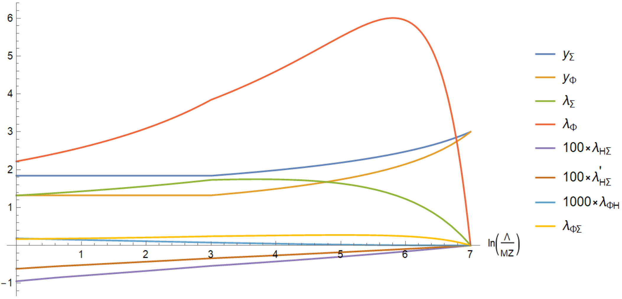
Figure 1: A typical solution of the RGEs for $y_{0}=3$, $\Lambda=\mathrm{e}^{7}M_{Z}\approx 100\mathrm{\,TeV}$ and $M_{R}=\mathrm{e}^{3}M_{Z}\approx 1.8\mathrm{\,TeV}$.

The Yukawa parameters $y_{\Sigma}$ and $y_{\Phi}$, starting from their value $y_{0}$ given by the boundary condition (37) at the compositeness scale $\Lambda$, do not run to small $\ll 1$ values. Typically, they are

$$y_{\Sigma}(M_{R}) \simeq 1\,,$$ (84)

$$y_{\Phi}(M_{R}) \simeq 1\,.$$ (85)

Such estimate is in fact rather robust Bardeen et al. (1990); Cvetic (1999), since it is sensitive only very weakly to the high-energy values of $y_{\Sigma}$ and $y_{\Phi}$, and exhibiting the typical behavior in the presence of an infrared fixed point, which is demonstrated in the Fig. 2. We can see that a rather wide range of high-energy Yukawa parameter values, $y_{0}\in(3,30)$, is squeezed by RGE evolution into a quite small range of low-energy values, $y_{\Sigma}(M_{R})\in(1.8,2.6)$ and $y_{\Phi}(M_{R})\in(1.1,1.4)$.

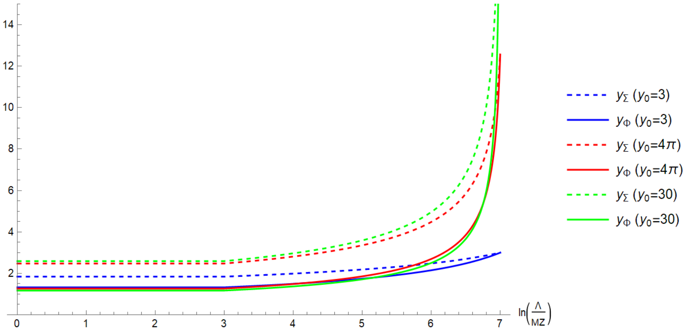
Figure 2: A solution for $y_{\Sigma}$ and $y_{\Phi}$ of the RGEs for the boundary conditions (37) given by three values $y_{0}=3,4\pi,30$, and for $\Lambda=\mathrm{e}^{7}M_{Z}\approx 100\mathrm{\,TeV}$ and $M_{R}=\mathrm{e}^{3}M_{Z}\approx 1.8\mathrm{\,TeV}$.

On the other hand, the neutrino Yukawa coupling $y_{H}$ is not generated dynamically, and therefore, it is not subject to any boundary condition at $\Lambda$. Thus, its value, $y_{H}(M_{R})$, is a free parameter to be fixed from phenomenology. In particular, we will fix it later by arguments of successful leptogenesis.

All the scalar quartic couplings $\lambda$’s, except for $\lambda_{H}$, are generated dynamically, and fixed by the high-energy boundary conditions (38). To determine the mass spectrum of the Higgs bosons we need to know the low-energy values of these quartic couplings, which are solutions of the corresponding RGEs given in Appendix C. Our analysis of their solutions in a wide range of the free model parameters shows that the quartic couplings typically demonstrate the following hierarchy

$$\lambda_{\Sigma},\lambda_{\Phi}(M_{Z}) \sim \ \mathcal{O}(1)\,,$$ (86)

$$\lambda_{\Phi\Sigma}(M_{Z}) \sim \ \mathcal{O}(10^{-1})\,,$$ (87)

$$\lambda_{H\Sigma},\lambda^{\prime}_{H\Sigma}(M_{Z}) \sim -\mathcal{O}(10^{-2})\,,$$ (88)

$$\lambda_{\Phi H}(M_{Z}) \sim \ \mathcal{O}(10^{-4})\,.$$ (89)

The $\kappa$ parameter is also generated dynamically. It is fixed by the high-energy boundary condition (39), and its magnitude is driven mainly by the last term in Eq. (C), as can be seen from

$${\color[rgb]{0,0,0}\mathrm{D}\kappa} = \kappa f-8\,y_{H}\,y_{\Sigma}\,y_{\Phi}\,M_{R}\,,$$ (90)

where

$$f=2\lambda_{\Phi H}+2\lambda_{\Phi\Sigma}+2\lambda_{H\Sigma}+4\lambda^{\prime}_{H\Sigma}-\tfrac{3}{2}\big{(}3g_{2}^{2}+g_{1}^{2}\big{)}+y_{H}^{2}+y_{\Sigma}^{2}+2y_{\Phi}^{2}+3y_{t}^{2}\,.$$ (91)

Since the last term drops off below the heavy neutrino decoupling scale $M_{R}$, the evolution of $\kappa$ saturates at this point. Therefore, in order to estimate the magnitude of $\kappa$ it is sufficient to calculate its value at $M_{R}$. Neglecting the scale dependence of all the other parameters, we can write

$$\kappa(M_{R})\approx\frac{8\,y_{H}\,y_{\Sigma}\,y_{\Phi}}{f}\left[1-\left(\frac{M_{R}}{\Lambda}\right)^{f/16\pi^{2}}\right]M_{R}\ \sim y_{H}M_{R}\,.$$ (92)

The last very rough estimate is obtained from our numerical analysis of the low-energy values of the model Yukawa, gauge and quartic coupling constants. It follows that typically $f\sim\mathcal{O}(10)$, so the exponent in the second term is $<1$, but not $\ll 1$. Then taking into account (18) we neglect the second term in the square bracket. Since the ratio $8\,y_{\Sigma}\,y_{\Phi}/f$ is of order $\mathcal{O}(1)$, we come up with the above-mentioned rough estimate.

VI.2 Fixing of parameters related to the SM

The Higgs-doublet VEVs must satisfy

$$v=\sqrt{v_{H}^{2}+v_{\Sigma}^{2}}\doteq 246\mathrm{\,GeV}\,,$$ (93)

in order to get the correct values for the masses of $W$ and $Z$. To achieve the hierarchy, from Eq. (3) or (2) and taking into account the value of the Yukawa parameter $y_{\Sigma}$ in Eq. (84), the hierarchy of the VEVs $v_{\Sigma}\ll v_{H}$ is required. From that we can set

$$v_{H}\simeq v\doteq 246\mathrm{\,GeV}\,.$$ (94)

Based on this, in order to reproduce the mass of the top quark as

$$m_{t}=y_{t}(m_{t})\,v_{H}/\sqrt{2}\doteq 174\mathrm{\,GeV}.$$ (95)

the fixing of the top-quark Yukawa parameter as

$$y_{t}(m_{t})\approx\frac{\sqrt{2}m_{t}}{v_{H}}\doteq 1\,,$$ (96)

is required, just as in the SM.

The quartic coupling parameter of the elementary Higgs boson, $\lambda_{H}$, is fixed by the phenomenological requirement to reproduce the SM-like Higgs boson mass, $m_{h^{0}}\doteq 125\mathrm{\,GeV}$. The mass of the SM-like Higgs boson in our model is approximately given by Eq. (73), which leads to

$$\lambda_{H}(m_{h^{0}})\simeq\frac{m_{h^{0}}^{2}}{v_{H}^{2}}\doteq 0.26\,.$$ (97)

Therefore, we should set the initial value $\lambda_{H}(\Lambda)$ in a way that $\lambda_{H}(m_{h^{0}})$ gets the value stated in Eq. (97). On the other hand $\lambda_{H}(\Lambda)$ should not be negative, since otherwise the ground state of the model would be unstable. The one-loop RGEs show that the small value of $\lambda_{H}(m_{h^{0}})$ presented in (97), requires that the initial value $\lambda_{H}(\Lambda)$ be negative, unless

$$\Lambda\leq 100\mathrm{\,TeV}\,.$$ (98)

This feature of our model is practically the same as in the SM, where the one-loop RGEs exhibit the same limit on the vacuum stability. Nevertheless, the three-loop level RGEs of the SM show Degrassi et al. (2012) that the vacuum stability limit is, in fact, pushed to much higher scales. Although we expect the same behavior in our model, to be on the safe side we set the value of the compositeness scale to be

$$\Lambda=100\mathrm{\,TeV}\,.$$ (99)

Notice that the RGE solutions are weakly sensitive to the actual value of $\Lambda$.

VI.3 Constraint from additional Higgs bosons

As we already saw that our model contains extra Higgses. In order to pass the existing experimental constraints Tanabashi et al. (2018) they must be either sufficiently heavy, i.e., with masses greater than $500\mathrm{\,GeV}$, or sufficiently weakly coupled to the known SM particles, i.e., the light states should be predominantly made of sterile $\Phi$ fields with only a small admixtures of electroweak doublets $H$ and $\Sigma$ fields. From these constraints, a large ratio

$$\frac{v_{\Phi}}{v_{\Sigma}}\equiv r_{\Phi\Sigma}\gg 1$$ (100)

can be advocated as follows.

Assuming the hierarchy $v_{\Sigma},v_{\Phi}\ll v_{H},\kappa$ and using the estimate (92) in Eq. (57), we get an expression for the charged Higgs boson mass

$$m_{h^{\pm}}^{2} \approx \frac{v_{H}}{2}\Big{(}\sqrt{2}\,r_{\Phi\Sigma}\,M_{R}\,y_{H}-\lambda^{\prime}_{H\Sigma}\,v_{H}\Big{)}\,.$$ (101)

If the second term is larger in magnitude than the first one, we would have the problem of having a too light charged Higgs boson with mass $\sim 0.1v$, according to the estimate in Eq. (88). The first term contains the product $M_{R}\,y_{H}$, which in our seesaw scenario easily turns out to be of the same order of magnitude as $v$ or even smaller. Therefore, to make the first term dominant in Eq. (101), we need $r_{\Phi\Sigma}$ to be large enough, as indicated in Eq. (100).

Among the pseudo-scalars there is the majoron $\eta^{0}$, which is a massless Nambu–Goldstone boson of the spontaneously broken $U_{L}(1)$. In order to make it phenomenologically harmless, we require that it should be dominated by the SM singlet $a_{\Phi}^{0}$ state. From Eq. (72) and Eq. (175) we see that the majoron $\eta^{0}$ does not contain $a_{H}^{0}$ component, and therefore, we only need to suppress the $a_{\Sigma}^{0}$ admixture, requiring again the condition given in Eq. (100).

However, the massive pseudo-scalar $a^{0}$ cannot be made sterile, hence we must guarantee it to be sufficiently heavy in order to pass the experimental constraints from the neutral Higgs non-observation Tanabashi et al. (2018). The approximate value of its mass, under the assumption of the hierarchy $v_{\Sigma},v_{\Phi}\ll v_{H},\kappa$, is

$$m_{a^{0}}^{2}\approx\left(r_{\Phi\Sigma}+\frac{1}{r_{\Phi\Sigma}}\right)\frac{y_{H}}{\sqrt{2}}v_{H}M_{R}\,.$$ (102)

Therefore, to make $a^{0}$ heavy we have now two possibilities for $r_{\Phi\Sigma}$, either very large or very small, and then to be compatible with the previous requirements we are again led to Eq. (100).

A similar situation takes place in the sector of the $H^{0}$ and $s^{0}$ Higgs bosons. From Eq. (74) and Eq. (75), using Eq. (92) we have that their masses are

$$m_{H^{0}}^{2}\approx\left(r_{\Phi\Sigma}+\frac{1}{r_{\Phi\Sigma}}\right)\frac{y_{H}}{\sqrt{2}}v_{H}M_{R}\,.$$ (103)

and

$$m_{s^{0}}\ll m_{h^{0}}\,.$$ (104)

Analogously to Eq. (102), a large value of $r_{\Phi\Sigma}$ allows making $H^{0}$ sufficiently heavy, in accordance with the current experimental constraints Tanabashi et al. (2018). However, the scalar $s^{0}$ is unavoidably light (104) and, therefore, must be predominantly sterile. As follows from Eqs. (82) and (181), this condition is satisfied for large values of $r_{\Phi\Sigma}$ (100), and then, under the hierarchy $v_{\Sigma}\ll v_{\Phi}\ll v_{H}$ and $r_{\Phi\Sigma}\gg 1$ and $\lambda_{\Phi H}\ll\lambda_{H}$, the $s^{0}$-boson mass can be approximated by

$$m_{s^{0}}^{2}\approx\lambda_{\Phi}v_{\Phi}^{2}\,.$$ (105)

Let us summarize this section. In order to satisfy the phenomenological requirements it is necessary to consider large values of $r_{\Phi\Sigma}$ (100). Then we can identify two groups of Higgs bosons:

• Light Higgs bosons: the SM-like Higgs boson $h^{0}$, made mostly of the elementary electroweak doublet $H$ field; a very light scalar $s^{0}$ and massless majoron $\eta^{0}$, both made mostly of the singlet $\Phi$. Their masses at the electroweak scale are

  $$m_{h^{0}}^{2} \approx \lambda_{H}v_{H}^{2}\,,$$ (106)

  $$m_{s^{0}}^{2} \approx \lambda_{\Phi}v_{\Phi}^{2}\,,$$ (107)

  $$m_{\eta^{0}}^{2} = 0\,,$$ (108)

• Heavy Higgs bosons: $X=h^{\pm},\,a^{0},\,H^{0}$, which are all made mostly of the electroweak doublet $\Sigma$ and have almost degenerate masses above the electroweak scale:

  $$m_{X}^{2} \approx r_{\Phi\Sigma}m_{D}M_{R}\,.$$ (109)

VI.4 Constraints from Leptogenesis

Leptogenesis renders stringent constraints on the free parameters (83) of our model. The Sakharov conditions for the case of leptogenesis are: 1) LNV processes are allowed, 2) they are $CP$ asymmetric, 3) before they become cosmologically irrelevant during the evolution of the Universe they go out of thermal equilibrium. Obviously, the condition 1) is satisfied in our model. As to the condition 2), in the simplified version of our model with only one fermion generation, which we are studying here, $CP$ is conserved. However, $CP$ violation (CPV) can be easily accommodated in the realistic models of any seesaw scenario, since there are several leptonic Yukawa coupling constants in the neutrino mass matrix which are complex, leading to the physical CPV phases. However, the resulting CPV effect may not be sufficiently strong for successful leptogenesis. In order to enhance the CPV one has to either push the masses of the heavy Majorana neutrinos (5) to very large values $>10^{9}\mathrm{\,GeV}$ Buchmuller and Plumacher (1996), or introduce a pair of quasi-degenerate heavy Majorana neutrinos, leading to resonant enhancement of the CPV in their LNV decays Pilaftsis (1997). The first option is not pertinent for our model, due to Eqs. (18) and (98). Meanwhile, the second option is naturally realizable in our model, as in any other model with a low-scale seesaw. The resonant condition providing the maximal CPV effect

$$\frac{\Gamma_{N}}{2}\simeq|m_{N_{+}}-m_{N_{-}}|$$ (110)

relates the mass splitting of the heavy Majorana neutrinos and their decay rate $\Gamma_{N}$.

Condition 3) requires that the expansion rate of the Universe, quantified by the temperature-dependent Hubble parameter $H(T)$, is larger than the decay rate of the heavy Majorana neutrinos,

$$H(T=m_{N_{+}})\gtrsim\frac{\Gamma_{N}}{2}\,.$$ (111)

The Hubble parameter at a temperature $T$ for a given extension of the SM with $g_{*}$ degrees of freedom is $H(T)\sim 1.73\sqrt{g_{*}}T^{2}/\Lambda_{\mathrm{Planck}}$.

Our model contains a set of extra Higgs bosons, providing heavy Majorana neutrinos with several decay modes into the light neutrino relevant for leptogenesis. The total decay rate of the heavy Majorana neutrinos is given by

$$\Gamma_{N}\sim\sum_{i}\frac{y_{N\rightarrow i}^{2}}{8\pi}m_{N_{+}}\,,$$ (112)

where $y_{N\rightarrow i}$ is a coupling constant responsible for the $i$-th decay channel. They can be sorted into groups according to the boson emitted in the decay. Here we present approximate expressions for these couplings, derived with the assumption of the hierarchy $v_{\Sigma}\ll v_{\Phi}\ll v_{H}$ motivated in the previous sections.

• Light Higgs boson emission

  $$y_{N\rightarrow\nu h} \approx -\frac{y_{H}}{2}\,,$$ (113)

  $$y_{N\rightarrow\nu s} \approx \frac{1}{2r_{\Phi\Sigma}}y_{\Sigma}-\frac{m_{D}}{M_{R}}y_{\Phi}\,,$$ (114)

  $$y_{N\rightarrow\nu\eta} \approx \frac{1}{2r_{\Phi\Sigma}}y_{\Sigma}-\frac{m_{D}}{M_{R}}y_{\Phi}\,,$$ (115)

  $$y_{N\rightarrow eh} \approx y_{H}^{2}\frac{v_{\Sigma}}{2M_{R}}\,.$$ (116)

• Heavy Higgs boson $X=a^{0},\,H^{0}$ emission

  $$y_{N\rightarrow\nu X} \approx -\frac{y_{\Sigma}}{2}\,.$$ (117)

• The SM Gauge boson emission

  $$y_{N\rightarrow\nu Z} \approx \frac{m_{D}}{\sqrt{2}M_{R}}\frac{g}{2\cos{\theta_{W}}}\,,$$ (118)

  $$y_{N\rightarrow eW} \approx \frac{m_{D}}{\sqrt{2}M_{R}}\frac{g}{\sqrt{2}}\,,$$ (119)

In most of the model realizations of the leptogenesis with resonant $CP$ asymmetry enhancement, it is not necessary to tune the model parameters exactly to the resonance given by (110). It is enough to be in the vicinity of the resonance. According to the numerical analysis in Pilaftsis (1997) performed for $m_{N_{\pm}}=10\mathrm{\,TeV}$ and $|y_{N}|\sim 10^{-6}$, the mass splitting of the heavy neutrinos

$$\frac{|m_{N_{+}}-m_{N_{-}}|}{m_{N_{+}}}\sim 10^{-7}\,$$ (120)

is sufficient. In a more recent analysis in Iso et al. (2011), where a wash-out effect mediated by $Z^{\prime}$ with mass $\sim M_{N}$ is taken into account, a stronger $CP$ asymmetry is needed requiring several orders of magnitude smaller mass splitting than in Eq. (120). In our scheme similar wash-out effects can be expected due to the interaction channels mediated by the heavy Higgs bosons with mass $\sim M_{N}$. However to reliably address the wash-out effects requires a detailed analysis within a realistic version of our model, which we leave for future work. For now we take (120) as a numerical input to our analysis, keeping in mind that if needed the mass splitting can be made correspondingly smaller by pushing $v_{\Phi}$ to lower values.

Estimating approximately the number of degrees of freedom in our model for the realistic 3-generation case to be $g_{*}\approx 100$ we obtain an upper bound for the coupling constants

$$y_{N\rightarrow i}\lesssim 10^{-7}\left[\frac{m_{N_{+}}}{\mathrm{\,TeV}}\right]\,.$$ (121)

The right-handed neutrino mass parameter $M_{R}$ is among the free parameters, ranging in our model roughly from $\sim 1\mathrm{\,TeV}>v$ up to $\lesssim 100\mathrm{\,TeV}=\Lambda$. In order to be specific let us consider a benchmark scenario in our model with

$$M_{R}=10\mathrm{\,TeV}\,.$$ (122)

which enable us to relate directly our analysis to the conclusions of Ref. Pilaftsis (1997).

Now, all the coupling constants (113)-(119) must satisfy the out-of-equilibrium condition (121). Therefore, the Yukawa parameter $y_{H}$ at the scale $M_{R}$ must be set at such a small value that the coupling constant (113) satisfies (121), so we choose

$$y_{H}(M_{R})\approx 10^{-7}\,,$$ (123)

and with this value we calculate from (122) and (14) the ratio

$$\frac{m_{D}}{M_{R}}\approx 10^{-9}\,.$$ (124)

Next we observe that the Yukawa coupling constants to heavy neutrinos (117) are unavoidably large, a consequence of the dynamical origin of the Yukawa parameters $y_{\Sigma}$ and $y_{\Phi}$, which are of the order $\mathcal{O}(1)$ as a result of the RGE running from their large value at the compositeness scale $\Lambda$. Therefore, the only possibility to prevent the decay rate of the heavy neutrinos from being unbearably large is to forbid the decay channels to heavy Higgs bosons kinematically by the condition $m_{X}>m_{N}$. Using the expression for the masses of heavy Higgs bosons (109) and for heavy neutrinos $m_{N}\sim M_{R}$, we obtain the condition

$$r_{\Phi\Sigma}>\frac{M_{R}}{m_{D}}\,.$$ (125)

Taking the ratio (124) into account, we estimate $r_{\Phi\Sigma}$ conservatively as

$$r_{\Phi\Sigma}\approx 10^{9}\,.$$ (126)

Now, in order to obtain the necessary CPV magnitude for successful leptogenesis, the mass splitting of the quasi-degenerate heavy neutrinos has to be at least of the order $10^{-7}$, see (120). From (5) we see that the mass splitting is dominated by the inverse-seesaw mass parameter $\mu_{\mathrm{inv}}$

$$|m_{N_{+}}-m_{N_{-}}|\approx\mu_{\mathrm{inv}}=\frac{y_{\Phi}v_{\Phi}}{\sqrt{2}}\,.$$ (127)

Provided that $y_{\Phi}\sim 1$, the mass splitting constrains the VEV of the SM singlet scalar $\Phi$ to

$$v_{\Phi}\leq 10^{-7}M_{R}\,.$$ (128)

To be more safe with leptogenesis we may choose in Eq. (120) the mass splitting to be $10^{-8}$, which leads to

$$v_{\Phi}\approx 100\mathrm{\,keV}\,.$$ (129)

From (126) we obtain

$$v_{\Sigma}\approx 0.1\mathrm{\,meV}\,.$$ (130)

Let us summarize our order-of-magnitude estimates of the couplings constants (113)-(119), motivated by successful leptogenesis:

$$y_{N\nu s} \approx 10^{-9}\,,$$ (131)

$$y_{N\nu\eta} \approx 10^{-9}\,,$$ (132)

$$y_{N\nu Z} \approx 10^{-9}\frac{g}{2\cos{\theta_{W}}}\,,$$ (133)

$$y_{NeW} \approx 10^{-9}\frac{g}{\sqrt{2}}\,,$$ (134)

$$y_{Neh} \approx 10^{-31}\,.$$ (135)

This completes the estimation of the free parameters of our model and in what follows we will discuss some of its predictions.

VII Prediction of the model

With the parameters of our model approximately evaluated in the previous sections, we can derive its key predictions and compare with the existing experimental data. As will be seen, there is a small room to play with the parameters within the ballpark of the approximations made in these evaluations. Therefore, the model is predictive and falsifiable.

VII.1 Light neutrino mass

The tiny active neutrino mass is given by Eq. (43) in terms of the Weinberg parameters, $w_{\mathrm{inv}},w_{\mathrm{lin}}$, rather than the Yukawa couplings. Since the RGE running of these Weinberg parameters is quite moderate, their order of magnitude stays the same over large interval of scales, from $M_{R}$ down to $m_{\nu}$. Therefore, in order to estimate the neutrino mass it is sufficient to consider just the initial values of the Weinberg parameters at the scale $M_{R}$, given in Eqs. (45) and (46). Inserting these values into (43) and applying (14) we obtain

$$m_{\nu}\approx\frac{v_{\Phi}}{\sqrt{2}}\frac{m_{D}}{M_{R}}\left(\frac{m_{D}}{M_{R}}y_{\Phi}-\frac{2}{r_{\Phi\Sigma}}y_{\Sigma}\right)\lesssim 10^{-13}\mathrm{\,eV}\,,$$ (136)

where in the numerical estimation we used (124), (126) and (129). Thus, the model predicts an extremely light active neutrino. It is important to note that this prediction can hardly be avoided in the present single-generation version of the model. In the case of the realistic three-generation version of the model we expect (136) to be applicable to the lightest neutrino mass eigenstate, and then, if the model satisfies the neutrino oscillation data global fit de Salas et al. (2018), it predicts that the neutrinoless double beta decay parameter $m_{\beta\beta}$ lies in the range 1.2 meV $\lesssim m_{\beta\beta}\lesssim$ 3.5 meV for the normal neutrino mass ordering and 15 meV $\lesssim m_{\beta\beta}\lesssim$ 50 meV for the inverted one. This is a generic result for such a small values (136) of the lightest neutrino state.

VII.2 Prediction for dark matter

There is only one Dark Matter (DM) particle candidate in our model: the scalar $s^{0}$ specified in Eq. (82) as a mixture of the electroweak doublet and singlet fields. Using the parameter fixing from the last section VI we estimate its mass from (107), (129) and (86)

$$m_{s}\approx 100\mathrm{\,keV}\,.$$ (137)

This is a nearly sterile state having only a tiny admixture of the doublets $H,\Sigma$ estimated as

$$|\mathrm{mix}(H\in s^{0})| \approx \frac{\lambda_{\Phi H}v_{H}v_{\Phi}-\sqrt{2}y_{H}M_{R}v_{\Sigma}}{\lambda_{H}v_{H}^{2}}\approx 10^{-10}\,,$$ (138)

$$|\mathrm{mix}(\Sigma\in s^{0})| \approx \frac{v_{\Sigma}}{\sqrt{v_{\Sigma}^{2}+v_{\Phi}^{2}}}\sim\frac{1}{r_{\Phi\Sigma}}\approx 10^{-9}\,.$$ (139)

In order to be a viable DM candidate its lifetime $\tau_{s}$ must be greater than the age of the Universe $\tau_{u}$. Thus, we impose on the $s^{0}$ total decay rate $\Gamma_{s}$ the cosmological upper bound

$$\frac{1}{\tau_{s}}=\Gamma_{s}\lesssim\frac{1}{\tau_{u}}\approx 10^{-33}\mathrm{\,eV}\,.$$ (140)

According to the recent analysis of the decaying warm DM performed in Ref. Kuo et al. (2018), the DM decay rate should be smaller by other two or tree orders of magnitude over the result (140), for successfully reproducing the DM abundance of the Universe of today.

For the mass value (86) the only kinematically allowed decay channel is

$$s^{0}\longrightarrow\nu\nu\,.$$ (141)

with the decay rate

$$\Gamma_{s\rightarrow\nu\nu} = \frac{y_{s\nu\nu}^{2}}{8\pi}m_{s}\,.$$ (142)

and with the corresponding Yukawa coupling

$$y_{s\nu\nu} = \sqrt{2}y_{\Sigma}\frac{m_{D}}{M_{R}}\left(\frac{1}{r_{\Phi\Sigma}}-\frac{m_{D}}{M_{R}}\right)\approx 10^{-18}\,,$$ (143)

which we evaluated, using (124) and (126), with the result

$$\Gamma_{s}\approx 10^{-32}\mathrm{\,eV}\,,$$ (144)

assuming no significant cancelation between two terms in (143). In our model, we can make the $s$-boson more stable by assuming an even more profound hierarchy than in (124), (125), or by fine-tuning the free parameters, e.g. $y_{H}$, to cancel the dominant term in $y_{s\nu\nu}$ (143), or by making the mass of the $s^{0}$ boson $m_{s}\propto v_{\Phi}$ smaller. The later option requires pushing $v_{\Phi}$ down, which eventually increases $CP$ assymmetry for the sake of leptogenesis as discussed above. We present such benchmark parameter setting in Tab.2 denoted as CP10. The second option based on cancellation is demonstrated in Tab.2 as a benchmark parameter setting DMtuned1. As one can see there, $y_{s\nu\nu}$ is two orders of magnitude lower and even with opposite sign than in the benchmark parameter setting BASIC1, even though both benchmark settings have the same hierarchies $r_{\Phi\Sigma}$ and $m_{D}/M_{R}$.

VII.3 Missing energy in $Z$-boson decay

Looking at the mass spectrum of the model, we can identify a potentially dangerous decay of the $Z$ boson

$$Z\longrightarrow s^{0}f\bar{f}\,,$$ (145)

since $s^{0}$ is not a pure electroweak singlet, but it has an admixture of the electroweak doublets (82). Such decay process, if strong enough, would be visible at accelerators as the production of a fermion-antifermion pair plus missing energy carried away by $s^{0}$.

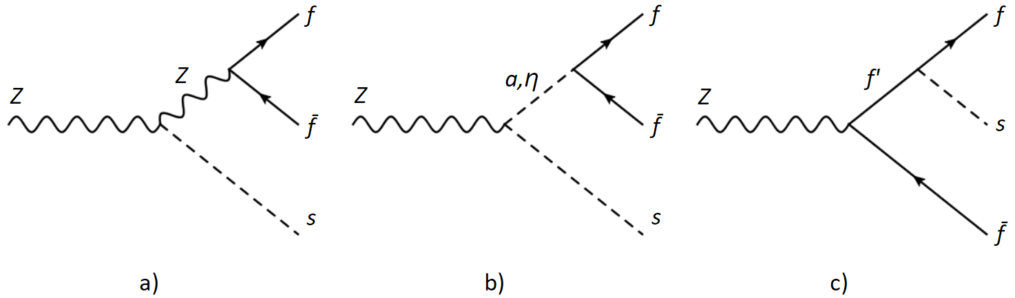
Figure 3: Feynman diagrams corresponding to the $Z$ boson decay $Z\longrightarrow s^{0}f\bar{f}$: a) exchange of virtual $Z$, b) exchange of virtual $a$ and $\eta$ and c) exchange of virtual fermion $f^{\prime}$.

The process $Z\rightarrow s^{0}f\bar{f}$ can be calculated from the tree-level amplitudes for which the exchange of virtual $Z$ boson, pseudoscalar $a$, majoron $\eta$ and fermion $f^{\prime}$ should be taken into account. We show the corresponding Feynman diagrams in the Fig. 3. For charged leptons in the final state, i.e., $f=\tau,\mu,e$, the amplitude of majoron exchange vanishes as their majoron Yukawa coupling constant is $y_{\eta ff}=0$. The amplitude for the fermion exchange is completely negligible as it is proportional to the Yukawa coupling parameter $y_{sff^{\prime}}\sim 10^{-18}$ being estimated to be approximately same as $y_{s\nu\nu}$ given in Eq. (143). The contribution from the amplitude of pseudoscalar exchange is not vanishing but negligibly small together with the corresponding Yukawa coupling constant

$$y_{aff}=\frac{gm_{f}}{\sqrt{2}M_{W}}\frac{v_{\Sigma}v_{\Phi}}{\sqrt{v_{H}^{2}v_{\Sigma}^{2}+v_{\Sigma}^{2}v_{\Phi}^{2}+v_{\Phi}^{2}v_{H}^{2}}}\approx\mathcal{O}(10^{-13})\,.$$ (146)

Therefore the dominant contribution comes from the $Z$ boson exchange, whose Yukawa $Zff$ coupling constant is roughly $y_{Zff}\approx\mathcal{O}(1)$, which has the most important suppression of its amplitude coming from the $H$ and $\Sigma$ mixing factors of the $s^{0}$ boson. Using the order-of-magnitude estimates from section VI, the admixture of the SM-like Higgs doublet $H$ is at the level of $\mathcal{O}(\frac{\lambda_{\Phi H}v_{\Phi}}{\lambda_{H}v_{H}})\sim 10^{-10}$ (see (184), (89) and (129)), and the admixture of the doublet $\Sigma$ is at the level of $\mathcal{O}(1/r_{\Phi\Sigma})\sim 10^{-9}$ (126). Assuming the $\Sigma$ admixture as the leading one, the partial decay rate for the process $Z\rightarrow s^{0}f\bar{f}$ can be estimated as

$$\Gamma_{Z\rightarrow s^{0}f\bar{f}}\approx\frac{1}{r_{\Phi\Sigma}^{2}}10^{-3}\mathrm{\,GeV}\,.$$ (147)

This gives a negligible branching ratio

$$B_{Z\rightarrow s^{0}f\bar{f}}\equiv\frac{\Gamma_{Z\longrightarrow s^{0}f\bar{f}}}{\Gamma_{Z}}\approx 10^{-21}\,,$$ (148)

compatible with the experimental data Tanabashi et al. (2018). Here $\Gamma_{Z}\doteq 2.5\mathrm{\,GeV}$ is the total decay width of the $Z$ boson.

For the same reason, namely because of smallness of the electroweak non-singlet component of the $s^{0}$-boson, other invisible $Z$ boson decay channels like, e.g., $Z\rightarrow s^{0}s^{0}f\bar{f}$, are also totally negligible.

VIII Conclusions

In this work, the possibility of dynamical LNV and neutrino mass generation, based on neutrino condensation, has been considered. In order to proof this concept, a simplified model setup with a single neutrino generation, to wit, without neutrino flavor mixing, has been constructed and studied. This test setup also lacks $CP$ violation in the neutrino Yukawa sector, and then it invalidates itself from being able to describe leptogenesis. Nevertheless, we believe that it shares important qualitative features and the order-of-magnitude quantitative estimates with a realistic three-generation version of the model, which is going to be developed in a successive work.

In order to check the viability of our neutrino condensation model, we have borrowed realistic leptogenesis constraints on the size of the mass of quasi-degenerate heavy Majorana neutrinos, their mass splitting and decay rates. We assumed a combined inverse plus linear seesaw mechanism for the explanation of the active neutrino mass and kept the seesaw scale rather low, i.e., $M_{R}\sim 1-10\mathrm{\,TeV}$, in order stay in the ballpark of current and near-future collider experiments. The neutrino condensation dynamically generates the LNV mass entries of the seesaw mass matrix, as VEVs of composite additional Higgs fields. Their coupling parameters are generated dynamically and fixed completely by the underlying new dynamics, which provides the necessary attraction within the LNV neutrino-neutrino channels.

The main message of this work, based on order-of-magnitude estimates, is that, in spite of such tightly constrained scheme with limited room to play with its parameters, the model has the potential to predict viable values of active neutrino masses and the mass and decay rate of a dark matter particle candidate, while satisfying the parameter requirements of successful leptogenesis.

Acknowledgements

This work was supported by Fondecyt (Chile) under grants No. 1170171, No. 3150472, No. 1180232, No. 1190845 as well as CONICYT (Chile) Basal FB0821. The work was supported from European Regional Development Fund-Project Engineering Applications of Microworld Physics (No. CZ.02.1.01/0.0/0.0/16_019/0000766).

Appendix A Neutrino mass matrix diagonalization

We present here the eigenvalues of the full neutrino mass matrix in Eq. (1), i.e., including the non-zero $\mu^{\prime}_{\mathrm{inv}}$-entry, under the assumption of the hierarchy (3), which comes from our phenomenological analysis done in Sect. VI. Here, we add the assumption

$$\mu^{\prime}_{\mathrm{inv}}\sim\mu_{\mathrm{inv}}\,.$$ (149)

We perform an expansion of the mass eigenvalues in the following small parameters, dubbed as $\varepsilon$:

$$\varepsilon\sim\sqrt{\frac{\mu_{\mathrm{lin}}}{M_{R}}}\sim\frac{m_{D}}{M_{R}}\sim\frac{\mu_{\mathrm{inv}}}{M_{R}}\sim\frac{{\mu^{\prime}_{\mathrm{inv}}}}{M_{R}}\,,$$ (150)

To leading order in all of these small parameters the eigenvalues are

$$\frac{m_{\nu}}{M_{R}} \simeq \left(\frac{m_{D}}{M_{R}}-\frac{m_{D}^{3}}{M_{R}^{3}}\right)\left(\frac{\mu_{\rm inv}}{M_{R}}\frac{m_{D}}{M_{R}}-2\frac{\mu_{\rm lin}}{M_{R}}\right)$$

$$\quad\quad+\left(\frac{\mu_{\mathrm{lin}}^{2}}{M_{R}^{2}}-2\frac{\mu_{\mathrm{lin}}}{M_{R}}\frac{m_{D}}{M_{R}}\frac{\mu_{\mathrm{inv}}}{M_{R}}+\frac{m_{D}^{2}}{M_{R}^{2}}\frac{\mu_{\mathrm{inv}}^{2}}{M_{R}^{2}}\right)\frac{\mu^{\prime}_{\mathrm{inv}}}{M_{R}}+\mathcal{O}(\varepsilon^{5})\,,$$

$$\frac{m_{N_{\pm}}}{M_{R}} \simeq \pm 1+\frac{1}{2}\frac{(\mu_{\mathrm{inv}}+\mu^{\prime}_{\mathrm{inv}})}{M_{R}}\pm\frac{4m_{D}^{2}+(\mu_{\mathrm{inv}}-\mu^{\prime}_{\mathrm{inv}})^{2}}{8M_{R}^{2}}$$

$$\quad\quad-\frac{1}{2}\frac{m_{D}}{M_{R}}\left(\frac{\mu_{\rm inv}}{M_{R}}\frac{m_{D}}{M_{R}}-2\frac{\mu_{\rm lin}}{M_{R}}\right)+\mathcal{O}(\varepsilon^{3})\,.$$

The light neutrino mass, to leading order $\mathcal{O}(\varepsilon^{3})$ and heavy neutrino masses to order $\mathcal{O}(\varepsilon^{1})$, are given as

$$\frac{m_{\nu}}{M_{R}} \simeq \frac{\mu_{\rm inv}}{M_{R}}\frac{m_{D}^{2}}{M_{R}^{2}}-2\frac{\mu_{\rm lin}}{M_{R}}\frac{m_{D}}{M_{R}}\,,$$ (152)

$$\frac{m_{N_{\pm}}}{M_{R}} \simeq \pm 1+\frac{1}{2}\frac{\mu_{\mathrm{inv}}+\mu^{\prime}_{\mathrm{inv}}}{M_{R}}\,.$$ (153)

The expression (152) for light neutrino mass coincides with Eq. (4) and it does not depend on $\mu^{\prime}_{\mathrm{inv}}$, in accordance with Gavela et al. (2009); Blanchet et al. (2010); Blanchet and Di Bari (2012). That motivates our assumption of $\mu^{\prime}_{\mathrm{inv}}=0$, under which the expression (153) of heavy neutrino mass coincides with Eq. (4).

The neutrino mass eigenstates $(\nu,N_{-},N_{+})$ are linear combinations of the original fields

$$\left(\begin{array}[]{c}\nu\\ N_{-}\\ N_{+}\end{array}\right) \simeq \mathcal{U}_{\nu}\left(\begin{array}[]{c}\nu_{L}\\ \nu_{R}^{c}\\ S_{R}^{c}\end{array}\right)\,,$$ (160)

where $\mathcal{U}_{\nu}$ is the neutrino mixing matrix transforming the neutrino mass matrix (1) into its diagonal form $\mathcal{U}_{\nu}M_{\nu}\mathcal{U}_{\nu}^{\mathrm{T}}$. To lowest order of the $\varepsilon$-parameters the neutrino mixing matrix is

$$\mathcal{U}_{\nu} \simeq \left(\begin{array}[]{ccc}-1+\frac{m_{D}^{2}}{2M_{R}^{2}}&\frac{\mu_{\mathrm{lin}}}{M_{R}}-\frac{\mu_{\mathrm{inv}}m_{D}}{M_{R}^{2}}&\frac{m_{D}}{M_{R}}\\ \frac{m_{D}}{\sqrt{2}M_{R}}&-\frac{1}{\sqrt{2}}&\frac{1}{\sqrt{2}}\left(1-\frac{m_{D}^{2}}{2M_{R}^{2}}\right)\\ \frac{m_{D}}{\sqrt{2}M_{R}}&\frac{1}{\sqrt{2}}&\frac{1}{\sqrt{2}}\left(1-\frac{m_{D}^{2}}{2M_{R}^{2}}\right)\end{array}\right)\,.$$ (164)

Appendix B Higgs boson mass matrices

The mass matrices of the Higgs bosons are obtained by Eq. (55) from the effective potential (IV.2).

• The $(2\times 2)$ mass matrix of charged Higgs bosons is obtained from

  $$\Big{[}M_{\mathrm{charged}}^{2}\Big{]}_{ij}=\left.\frac{\partial^{2}}{\partial a_{i}^{-}\partial a_{j}^{+}}\mathcal{V}_{\mathrm{eff}}(0,0,a_{H}^{-},a_{H}^{+},0,0,a_{\Sigma}^{-},a_{\Sigma}^{+},0,0)\right|_{a_{H}^{\pm}=0,a_{\Sigma}^{\pm}=0}\,,\ \mathrm{for\ }i,j=H,\Sigma\,.$$ (165)

  The resulting mass matrix is

  $$M_{\mathrm{charged}}^{2}=\frac{1}{2}(\sqrt{2}v_{\Phi}\kappa-\lambda^{\prime}_{H\Sigma}v_{H}v_{\Sigma})\left(\begin{array}[]{cc}\frac{v_{\Sigma}}{v_{H}}&1\\ 1&\frac{v_{H}}{v_{\Sigma}}\end{array}\right)\,,$$ (166)

  which is transformed into the diagonal form $\mathcal{U}_{\mathrm{charged}}M_{\mathrm{charged}}^{2}\mathcal{U}_{\mathrm{charged}}^{\mathrm{T}}$ by means of the orthogonal matrix

  $$\mathcal{U}_{\mathrm{charged}}=\frac{1}{v}\left(\begin{array}[]{cc}-v_{H}&v_{\Sigma}\\ v_{\Sigma}&v_{H}\end{array}\right)\,.$$ (169)

• The $(3\times 3)$ mass matrix neutral pseudo-scalar Higgs bosons is obtained from

  $$\Big{[}M_{\mathrm{pseudo}}^{2}\Big{]}_{ij}=\left.\frac{\partial^{2}}{\partial a_{i}^{0}\partial a_{j}^{0}}\mathcal{V}_{\mathrm{eff}}(0,a_{H}^{0},0,0,0,a_{\Sigma}^{0},0,0,0,a_{\Phi}^{0})\right|_{a_{H}^{0}=0,a_{\Sigma}^{0}=0,a_{\Phi}^{0}=0}\,,\ \mathrm{for\ }i,j=H,\Sigma,\Phi\,.$$ (170)

  The resulting mass matrix is then

  $$M_{\mathrm{pseudo}}^{2}=\frac{\kappa}{\sqrt{2}}\left(\begin{array}[]{ccc}\frac{v_{\Sigma}v_{\Phi}}{v_{H}}&v_{\Phi}&v_{\Sigma}\\ v_{\Phi}&\frac{v_{H}v_{\Phi}}{v_{\Sigma}}&v_{H}\\ v_{\Sigma}&v_{H}&\frac{v_{H}v_{\Sigma}}{v_{\Phi}}\end{array}\right)\,,$$ (171)

  which is transformed into the diagonal form $\mathcal{U}_{\mathrm{pseudo}}M_{\mathrm{pseudo}}^{2}\mathcal{U}_{\mathrm{pseudo}}^{\mathrm{T}}$ by means of the orthogonal matrix

  $$\mathcal{U}_{\mathrm{pseudo}}=\left(\begin{array}[]{ccc}\frac{v_{H}}{v}&-\frac{v_{\Sigma}}{v}&0\\ 0&-\frac{v_{\Sigma}}{\sqrt{v_{\Sigma}^{2}+v_{\Phi}^{2}}}&\frac{v_{\Phi}}{\sqrt{v_{\Sigma}^{2}+v_{\Phi}^{2}}}\\ \frac{v_{\Sigma}v_{\Phi}}{\sqrt{v_{H}^{2}v_{\Sigma}^{2}+v_{\Sigma}^{2}v_{\Phi}^{2}+v_{\Phi}^{2}v_{H}^{2}}}&\frac{v_{\Phi}v_{H}}{\sqrt{v_{H}^{2}v_{\Sigma}^{2}+v_{\Sigma}^{2}v_{\Phi}^{2}+v_{\Phi}^{2}v_{H}^{2}}}&\frac{v_{H}v_{\Sigma}}{\sqrt{v_{H}^{2}v_{\Sigma}^{2}+v_{\Sigma}^{2}v_{\Phi}^{2}+v_{\Phi}^{2}v_{H}^{2}}}\end{array}\right)\,.$$ (175)

• The $(3\times 3)$ mass matrix neutral scalar Higgs bosons is obtained from

  $$\Big{[}M_{hHs}^{2}\Big{]}_{ij}=\left.\frac{\partial^{2}}{\partial h_{i}^{0}\partial h_{j}^{0}}\mathcal{V}_{\mathrm{eff}}(h_{H}^{0},0,0,0,h_{\Sigma}^{0},0,0,0,h_{\Phi}^{0},0)\right|_{h_{H}^{0}=0,h_{\Sigma}^{0}=0,h_{\Phi}^{0}=0}\,,\ \mathrm{for\ }i,j=H,\Sigma,\Phi\,.$$ (176)

  The resulting mass matrix is then

  $$M_{hHs}^{2}=\left(\begin{array}[]{ccc}\frac{v_{\Sigma}v_{\Phi}\kappa}{\sqrt{2}v_{H}}+v_{H}^{2}\lambda_{H}&-\frac{v_{\Phi}\kappa}{\sqrt{2}}+v_{H}v_{\Sigma}(\lambda_{H\Sigma}+\lambda^{\prime}_{H\Sigma})&-\frac{v_{\Sigma}\kappa}{\sqrt{2}}+v_{H}v_{\Phi}\lambda_{\Phi H}\\ -\frac{v_{\Phi}\kappa}{\sqrt{2}}+v_{H}v_{\Sigma}(\lambda_{H\Sigma}+\lambda^{\prime}_{H\Sigma})&\frac{v_{H}v_{\Phi}\kappa}{\sqrt{2}v_{\Sigma}}+v_{\Sigma}^{2}\lambda_{\Sigma}&-\frac{v_{H}\kappa}{\sqrt{2}}+v_{\Sigma}v_{\Phi}\lambda_{\Phi\Sigma}\\ -\frac{v_{\Sigma}\kappa}{\sqrt{2}}+v_{H}v_{\Phi}\lambda_{\Phi H}&-\frac{v_{H}\kappa}{\sqrt{2}}+v_{\Sigma}v_{\Phi}\lambda_{\Phi\Sigma}&\frac{v_{H}v_{\Sigma}\kappa}{\sqrt{2}v_{\Phi}}+v_{\Phi}^{2}\lambda_{\Phi}\end{array}\right)\,,$$ (177)

  which is transformed into the diagonal form $\mathcal{U}_{hHs}M_{hHs}^{2}\mathcal{U}_{hHs}^{\mathrm{T}}$ by means of the orthogonal matrix which, under the hierarchy $v_{\Sigma}\ll v_{\Phi}\ll v_{H}$ ($r_{\Phi\Sigma}\gg 1$) and $\lambda_{\Phi H}\ll\lambda_{H}$, is approximated as

  $$\mathcal{U}_{hHs}=\left(\begin{array}[]{ccc}1-\varepsilon_{H}&\varepsilon_{\Sigma}&\varepsilon_{\Phi}\\ \varepsilon_{\Sigma}&-\frac{v_{\Phi}}{\sqrt{v_{\Sigma}^{2}+v_{\Phi}^{2}}}&\frac{v_{\Sigma}}{\sqrt{v_{\Sigma}^{2}+v_{\Phi}^{2}}}\\ -\varepsilon_{\Phi}&\frac{v_{\Sigma}}{\sqrt{v_{\Sigma}^{2}+v_{\Phi}^{2}}}&\frac{v_{\Phi}}{\sqrt{v_{\Sigma}^{2}+v_{\Phi}^{2}}}\end{array}\right)\,,$$ (181)

  where

  $$\varepsilon_{H} = \frac{1}{2}\left(\frac{\big{(}\lambda_{\Phi H}v_{H}v_{\Phi}-\sqrt{2}\kappa v_{\Sigma}\big{)}^{2}}{\lambda_{H}^{2}v_{H}^{4}}-\frac{v_{\Sigma}^{2}}{v_{H}^{2}}\right)\,,$$ (182)

  $$\varepsilon_{\Sigma} = \frac{v_{\Sigma}}{v_{H}}\,,$$ (183)

  $$\varepsilon_{\Phi} = \frac{\lambda_{\Phi H}v_{H}v_{\Phi}-\sqrt{2}\kappa v_{\Sigma}}{\lambda_{H}v_{H}^{2}}\,.$$ (184)

Appendix C Renormalization Group Equations

We derived the Renormalization Group Equations (RGE), used in our analysis, with the help of the pyR@TE software Lyonnet et al. (2014); Lyonnet and Schienbein (2017).

The RGEs for the gauge coupling constants of hypercharge $g_{1}$, of $\mathrm{SU}(2)_{L}$ $g_{2}$, and of color $g_{3}$, are the same as for the two-Higgs-doublet models,

$$\mathrm{D}g_{1}=\hphantom{-}7g_{1}^{3}\,, g_{1}^{2}(M_{Z})\doteq 0.127\,,$$ (185a)

$$\mathrm{D}g_{2}=-3g_{2}^{3}\,, g_{2}^{2}(M_{Z})\doteq 0.425\,,$$ (185b)

$$\mathrm{D}g_{3}=-7g_{3}^{3}\,, g_{3}^{2}(M_{Z})\doteq 1.440\,,$$ (185c)

where

$$\mathrm{D}\equiv 16\pi^{2}\frac{\mathrm{d}}{\mathrm{d}t}\,$$ (186)

and $t$ is

$$t=\ln\frac{m}{M_{Z}}\,.$$ (187)

In the RGE evolution we neglect the effect of the Yukawa coupling constants other than the neutrino Yukawa couplings $y_{H}$, $y_{\Sigma}$ and $y_{\Phi}$ from Eq. (IV.2) and the SM Yukawa coupling of the top quark, $y_{t}$. The latter runs from the compositeness scale $\Lambda$ all the way down to the electroweak scale, according to the following RGE:

$$\mathrm{D}y_{t}=y_{t}\big{[}\tfrac{9}{2}y_{t}^{2}+\theta(t-t_{M_{R}})y_{H}^{2}-\tfrac{17}{12}g_{1}^{2}-\tfrac{9}{4}g_{2}^{2}-8g_{3}^{2}\big{]}\,,\\$$ (188)

where

$$t_{M}=\ln\frac{M}{M_{Z}}\,.$$ (189)

On the other hand, the neutrino Yukawa couplings run according to their RGEs

$$\mathrm{D}y_{H} = y_{H}\big{[}\tfrac{1}{2}\big{(}5y_{H}^{2}+y_{\Sigma}^{2}\big{)}+3y_{t}^{2}-\tfrac{3}{4}g_{1}^{2}-\tfrac{9}{4}g_{2}^{2}\big{]}\,,$$ (190)

$$\mathrm{D}y_{\Sigma} = y_{\Sigma}\big{[}\tfrac{1}{2}\big{(}5y_{\Sigma}^{2}+y_{H}^{2}+4y_{\Phi}^{2}\big{)}-\tfrac{3}{4}g_{1}^{2}-\tfrac{9}{4}g_{2}^{2}\big{]}\,,$$ (191)

$$\mathrm{D}y_{\Phi} = y_{\Phi}\big{(}6y_{\Phi}^{2}+2y_{\Sigma}^{2}\big{)}\,,$$ (192)

only down to the right-handed neutrino mass scale $M_{R}$, where the heavy neutrinos decouple. At that scale we trade the neutrino Yukawa coupling constants for the effective generalized non-renormalizable Weinberg operators. Here we write the RGEs only for the two operators which are relevant and give a leading order contribution to the active neutrino masses. They are

$$\mathrm{D}w_{H\Phi H} = w_{H\Phi H}\big{[}6\,\theta(t-t_{m_{t}})y_{t}^{2}+\lambda_{H}+2\lambda_{H\Phi}-3\,\theta(t-t_{M_{Z}})g_{2}^{2}\big{]}\,,$$ (193)

$$\mathrm{D}w_{H\Sigma} = w_{H\Sigma}\big{[}3\,\theta(t-t_{m_{t}})y_{t}^{2}+\lambda_{H\Sigma}+\lambda^{\prime}_{H\Sigma}-3\,\theta(t-t_{M_{Z}})g_{2}^{2}\big{]}\,.$$ (194)

Here we have introduced thresholds corresponding to $m_{t}$ and $M_{Z}$, because in order to determine the neutrino masses, we need to run the Weinberg parameters many orders of magnitude below the electroweak scale. Keeping the coupling constants $y_{t}$ and $g_{2}$ would affect the running of the Weinberg parameters significantly and unphysically.

The RGEs for the dimensionless couplings $\lambda$’s of the effective potential in Eq. (IV.2) are

$$\mathrm{D}\lambda_{H} = 12\lambda_{H}^{2}+4\lambda_{H\Sigma}^{2}+4\lambda_{H\Sigma}\lambda^{\prime}_{H\Sigma}+2{\lambda^{\prime}_{H\Sigma}}^{2}+2\lambda_{\Phi H}^{2}+$$ (195)

$$-3\lambda_{H}(3g_{2}^{2}+g_{1}^{2})+\frac{3}{2}g_{2}^{4}+\frac{3}{4}(g_{2}^{2}+g_{1}^{2})^{2}+$$

$$+4\lambda_{H}\big{[}\theta(t-t_{M_{R}})y_{H}^{2}+3y_{t}^{2}\big{]}-4\,\theta(t-t_{M_{R}})y_{H}^{4}-12y_{t}^{4}\,,$$

$$\mathrm{D}\lambda_{\Sigma} = 12\lambda_{\Sigma}^{2}+4\lambda_{H\Sigma}^{2}+4\lambda_{H\Sigma}\lambda^{\prime}_{H\Sigma}+2{\lambda^{\prime}_{H\Sigma}}^{2}+2\lambda_{\Phi\Sigma}^{2}+$$ (196)

$$-3\lambda_{\Sigma}(3g_{2}^{2}+g_{1}^{2})+\frac{3}{2}g_{2}^{4}+\frac{3}{4}(g_{2}^{2}+g_{1}^{2})^{2}+$$

$$+4\lambda_{\Sigma}\theta(t-t_{M_{R}})y_{\Sigma}^{2}-4\,\theta(t-t_{M_{R}})y_{\Sigma}^{4}\,,$$

$$\mathrm{D}\lambda_{H\Sigma} = 6\lambda_{H}\lambda_{H\Sigma}+2\lambda_{H}\lambda^{\prime}_{H\Sigma}+6\lambda_{H\Sigma}\lambda_{\Sigma}+2\lambda_{\Sigma}\lambda^{\prime}_{H\Sigma}+4\lambda_{H\Sigma}^{2}+2{\lambda^{\prime}_{H\Sigma}}^{2}+2\lambda_{\Phi H}\lambda_{\Phi\Sigma}+$$ (197)

$$-3\lambda_{H\Sigma}(3g_{2}^{2}+g_{1}^{2})+\frac{9}{4}g_{2}^{4}+\frac{3}{4}g_{1}^{4}-\frac{3}{2}g_{2}^{2}g_{1}^{2}+$$

$$+2\lambda_{H\Sigma}\big{[}\theta(t-t_{M_{R}})\big{(}y_{H}^{2}+y_{\Sigma}^{2}\big{)}+3y_{t}^{2}\big{]}\,,$$

$$\mathrm{D}\lambda^{\prime}_{H\Sigma} = 2\lambda_{H}\lambda^{\prime}_{H\Sigma}+2\lambda_{\Sigma}\lambda^{\prime}_{H\Sigma}+8\lambda_{H\Sigma}\lambda^{\prime}_{H\Sigma}+4{\lambda^{\prime}_{H\Sigma}}^{2}+$$ (198)

$$-3\lambda^{\prime}_{H\Sigma}(3g_{2}^{2}+g_{1}^{2})+3g_{2}^{2}g_{1}^{2}+$$

$$+2\lambda^{\prime}_{H\Sigma}\big{[}\theta(t-t_{M_{R}})\big{(}y_{\Sigma}^{2}+y_{H}^{2})+3y_{t}^{2}\big{]}-\tfrac{7}{2}\,\theta(t-t_{M_{R}})y_{H}^{2}y_{\Sigma}^{2}\,,$$

$$\mathrm{D}\lambda_{\Phi} = 10\lambda_{\Phi}^{2}+4\lambda_{\Phi H}^{2}+4\lambda_{\Phi\Sigma}^{2}+8\,\theta(t-t_{M_{R}})\lambda_{\Phi}y_{\Phi}^{2}-32\,\theta(t-t_{M_{R}})y_{\Phi}^{4}\,,$$ (199)

$$\mathrm{D}\lambda_{\Phi H} = 4\lambda_{\Phi H}^{2}+6\lambda_{H}\lambda_{\Phi H}+4\lambda_{\Phi}\lambda_{\Phi H}+4\lambda_{\Phi\Sigma}\lambda_{H\Sigma}+2\lambda_{\Phi\Sigma}\lambda^{\prime}_{H\Sigma}+$$ (200)

$$-\frac{3}{2}\lambda_{\Phi H}(3g_{2}^{2}+g_{1}^{2})+2\lambda_{\Phi H}\big{[}\theta(t-t_{M_{R}})\big{(}y_{H}^{2}+2y_{\Phi}^{2}\big{)}+3y_{t}^{2}\big{]}\,,$$

$$\mathrm{D}\lambda_{\Phi\Sigma} = 4\lambda_{\Phi\Sigma}^{2}+6\lambda_{\Sigma}\lambda_{\Phi\Sigma}+4\lambda_{\Phi}\lambda_{\Phi\Sigma}+4\lambda_{\Phi H}\lambda_{H\Sigma}+2\lambda_{\Phi H}\lambda^{\prime}_{H\Sigma}+$$ (201)

$$-\frac{3}{2}\lambda_{\Phi\Sigma}(3g_{2}^{2}+g_{1}^{2})+2\lambda_{\Phi\Sigma}\theta(t-t_{M_{R}})\big{(}y_{\Sigma}^{2}+2y_{\Phi}^{2}\big{)}-16\,\theta(t-t_{M_{R}})\,y_{\Phi}^{2}\,y_{\Sigma}^{2}\,.$$

Finally, the RGE for the dimensionfull coupling parameter $\kappa$ of the effective potential (IV.2) is

$$\mathrm{D}\kappa = \kappa\big{[}2\lambda_{\Phi H}+2\lambda_{\Phi\Sigma}+2\lambda_{H\Sigma}+4\lambda^{\prime}_{H\Sigma}-\tfrac{3}{2}\big{(}3g_{2}^{2}+g_{1}^{2}\big{)}$$

$$\ \ \ +\theta(t-t_{M_{R}})\big{(}y_{H}^{2}+y_{\Sigma}^{2}+2y_{\Phi}^{2}\big{)}+3y_{t}^{2}\big{]}-8\,\theta(t-t_{M_{R}})\,y_{H}\,y_{\Sigma}\,y_{\Phi}\,M_{R}$$

In the RGEs for the couplings $\lambda$’s and $\kappa$ we introduce just one threshold, corresponding to $M_{R}$. The thresholds around the electroweak scale do not play a significant role in determining the mass spectrum for the Higgs bosons, the top-quark and the electroweak gauge bosons, as they all lie in the same ballpark.

Appendix D Numerical solutions of the RGEs

We show here one of the viable examples of numerical solution of the model.

Input RGE boundary conditions:

$$\Lambda = 100\mathrm{\,TeV}$$ (203)

$$y_{\Sigma,\Phi}(\Lambda) = 3$$ (204)

$$\lambda_{\Sigma,\Phi,H\Sigma,H\Sigma^{\prime},\Phi H,\Phi\Sigma}(\Lambda) = 0$$ (205)

$$\kappa(\Lambda) = 0$$ (206)

Input SM parameters:

$$v = 246\mathrm{\,GeV}\ \ \longrightarrow\ \ v_{H}\doteq 246\mathrm{\,GeV}$$ (207)

$$m_{h^{0}} = 125\mathrm{\,GeV}\ \ \longrightarrow\ \ \lambda_{H}(m_{h})=0.258$$ (208)

$$m_{t} = 174\mathrm{\,GeV}\ \ \longrightarrow\ \ y_{t}(m_{t})\doteq 1.0003$$ (209)

In Table 2 we present four benchmark parameter settings. The benchmark parameter setting BASIC10 corresponds to our order-of-magnitude estuimate performed in the section Sec. VI. The BASIC1 setting is included in order to show the impact of decreasing the value of $M_{R}$. The DMtuned1 setting is shown in order to demonstrate the cancellation in the DM decay Yukawa coupling constant $y_{s\nu\nu}$ from Eq. (143). The CP10 setting is included in order to show the impact of requirement to increase the $CP$ assymmetry up to the level $\sim 0.01$.

benchmark param. sets	BASIC10	BASIC1	DMtuned1	CP10
$\ M_{R}[\mathrm{\,TeV}]$	$10$	$1.11$	$1.11$	$10$
$\ v_{\Phi}[\mathrm{\,keV}]$	$120$	$120$	$0.1$	$0.012$
$\ r_{\Phi\Sigma}\ ||\ v_{\Sigma}[\mathrm{\,meV}]$	$1.2\times 10^{9}\ ||\ 0.1$	$1.2\times 10^{8}\ ||\ 1$	$10^{8}\ ||\ 0.001$	$1.2\times 10^{9}\ ||\ 0.00001$
$\ y_{H}(M_{R})\ ||\ m_{D}[\mathrm{\,keV}]$	$10^{-7}\ ||\ 17.4$	$10^{-7}\ ||\ 17.4$	$0.9\times 10^{-7}\ ||\ 15.7$	$10^{-7}\ ||\ 17.4$
$\ y_{\Sigma}(M_{R})\ ||\ \mu_{\mathrm{lin}}[\mathrm{\,meV}]$	$2.12\ ||\ 0.15$	$1.78\ ||\ 1.26$	$1.78\ ||\ 0.0013$	$2.12\ ||\ 0.000015$
$\ y_{\Phi}(M_{R})\ ||\ \mu_{\mathrm{inv}}[\mathrm{\,keV}]$	$0.17\ ||\ 1404$	$1.26\ ||\ 107$	$1.26\ ||\ 0.09$	$1.65\ ||\ 0.014$
$\ m_{\nu}^{(\mathrm{lin})}[\mathrm{\,eV}]$	$1.03\times 10^{-12}$	$0.08\times 10^{-9}$	$7.1\times 10^{-14}$	$1.03\times 10^{-16}$
$\ m_{\nu}^{(\mathrm{inv})}[\mathrm{\,eV}]$	$0.74\times 10^{-12}$	$0.05\times 10^{-9}$	$3.3\times 10^{-14}$	$0.74\times 10^{-16}$
$\ m_{\nu}[\mathrm{\,eV}]$	$0.29\times 10^{-12}$	$0.03\times 10^{-9}$	$3.9\times 10^{-14}$	$0.29\times 10^{-16}$
$\ \kappa(M_{Z})[\mathrm{\,MeV}]$	$0.57$	$0.09$	$0.083$	$0.57$
$\ \lambda_{H}(\Lambda)$	$0.0068$	$0.0068$	$0.0068$	$0.0068$
$\ \lambda_{\Sigma}(M_{Z})$	$1.151$	$1.356$	$1.356$	$1.151$
$\ \lambda_{\Phi}(M_{Z})$	$2.044$	$2.265$	$2.265$	$2.044$
$\ \lambda_{\Phi\Sigma}(M_{Z})$	$0.152$	$0.171$	$0.171$	$0.152$
$\ \lambda_{H\Sigma}(M_{Z})$	$-0.010$	$-0.009$	$-0.009$	$-0.010$
$\ \lambda^{\prime}_{H\Sigma}(M_{Z})$	$-0.006$	$-0.006$	$-0.006$	$-0.006$
$\ \lambda_{\Phi H}(M_{Z})$	$0.0002$	$0.0002$	$0.0002$	$0.0002$
$\ m_{H^{0},a^{0},h^{\pm}}[\mathrm{\,TeV}]$	$10.87$	$1.37$	$1.198$	$10.87$
$\ (m_{h^{\pm}}-m_{H^{0}})[\mathrm{\,MeV}]$	$2.5$	$38.4$	$45.4$	$2.5$
$\ (m_{H}-m_{a^{0}})[\mathrm{\,eV}]$	$0.0$	$0.0$	$0.0002$	$0.0018$
$\ y_{N\nu h}$	$5.0\times 10^{-8}$	$5.0\times 10^{-8}$	$4.5\times 10^{-8}$	$5.0\times 10^{-8}$
$\ y_{N\nu s}$	$2.0\times 10^{-9}$	$1.2\times 10^{-8}$	$0.9\times 10^{-8}$	$2.0\times 10^{-9}$
$\ y_{N\nu\eta}$	$2.0\times 10^{-9}$	$1.2\times 10^{-8}$	$0.9\times 10^{-8}$	$2.0\times 10^{-9}$
$\ m_{s^{0}}[\mathrm{\,keV}]$	$103$	$105$	$0.075$	$0.0089$
$\ y_{s\nu\nu}$	$-2.74\times 10^{-18}$	$-1.08\times 10^{-16}$	$1.43\times 10^{-18}$	$-2.74\times 10^{-18}$
$\ \Gamma_{s}[\mathrm{\,eV}]$	$3.06\times 10^{-32}$	$4.86\times 10^{-29}$	$6.12\times 10^{-36}$	$2.56\times 10^{-36}$

Table 2: Table of benchmark parameter settings.

References

- Davidson and Ibarra (2002) S. Davidson and A. Ibarra, Physics Letters B 535, 25 (2002), ISSN 0370-2693, URL http://www.sciencedirect.com/science/article/pii/S0370269302017355.
- Pilaftsis (1997) A. Pilaftsis, Phys. Rev. D56, 5431 (1997), eprint hep-ph/9707235.
- Asaka and Shaposhnikov (2005) T. Asaka and M. Shaposhnikov, Physics Letters B 620, 17 (2005), ISSN 0370-2693, URL http://www.sciencedirect.com/science/article/pii/S0370269305008087.
- Malinsky et al. (2005) M. Malinsky, J. C. Romao, and J. W. F. Valle, Phys. Rev. Lett. 95, 161801 (2005), eprint hep-ph/0506296.
- Martin (1991) S. P. Martin, Phys. Rev. D44, 2892 (1991).
- Antusch et al. (2003) S. Antusch, J. Kersten, M. Lindner, and M. Ratz, Nucl. Phys. B658, 203 (2003), eprint hep-ph/0211385.
- Smetana (2013a) A. Smetana, Eur. Phys. J. C73, 2513 (2013a), eprint 1301.1554.
- Smetana (2013b) A. Smetana, Ph.D. thesis, Charles U. (2013b), eprint 1309.4688, URL http://inspirehep.net/record/1254582/files/arXiv:1309.4688.pdf.
- Bardeen et al. (1990) W. A. Bardeen, C. T. Hill, and M. Lindner, Phys. Rev. D41, 1647 (1990).
- Cvetic (1999) G. Cvetic, Rev. Mod. Phys. 71, 513 (1999), eprint hep-ph/9702381.
- Hill et al. (1991) C. T. Hill, M. A. Luty, and E. A. Paschos, Phys. Rev. D43, 3011 (1991).
- Ivanov (2017) I. P. Ivanov, Progress in Particle and Nuclear Physics 95, 160 (2017), ISSN 0146-6410, URL http://www.sciencedirect.com/science/article/pii/S0146641017300327.
- Chalons and Domingo (2012) G. Chalons and F. Domingo, Phys. Rev. D 86, 115024 (2012), URL https://link.aps.org/doi/10.1103/PhysRevD.86.115024.
- Tanabashi et al. (2018) M. Tanabashi, K. Hagiwara, K. Hikasa, K. Nakamura, Y. Sumino, F. Takahashi, J. Tanaka, K. Agashe, G. Aielli, C. Amsler, et al. (Particle Data Group), Phys. Rev. D 98, 030001 (2018), URL https://link.aps.org/doi/10.1103/PhysRevD.98.030001.
- Degrassi et al. (2012) G. Degrassi, S. Di Vita, J. Elias-Miro, J. R. Espinosa, G. F. Giudice, G. Isidori, and A. Strumia, JHEP 08, 098 (2012), eprint 1205.6497.
- Buchmuller and Plumacher (1996) W. Buchmuller and M. Plumacher, Phys. Lett. B389, 73 (1996), eprint hep-ph/9608308.
- Iso et al. (2011) S. Iso, N. Okada, and Y. Orikasa, Phys. Rev. D83, 093011 (2011), eprint 1011.4769.
- de Salas et al. (2018) P. F. de Salas, D. V. Forero, C. A. Ternes, M. Tortola, and J. W. F. Valle, Phys. Lett. B782, 633 (2018), eprint 1708.01186.
- Kuo et al. (2018) J.-L. Kuo, M. Lattanzi, K. Cheung, and J. W. F. Valle (2018), eprint 1803.05650.
- Gavela et al. (2009) M. B. Gavela, T. Hambye, D. Hernandez, and P. Hernandez, JHEP 09, 038 (2009), eprint 0906.1461.
- Blanchet et al. (2010) S. Blanchet, T. Hambye, and F.-X. Josse-Michaux, JHEP 04, 023 (2010), eprint 0912.3153.
- Blanchet and Di Bari (2012) S. Blanchet and P. Di Bari, New J. Phys. 14, 125012 (2012), eprint 1211.0512.
- Lyonnet et al. (2014) F. Lyonnet, I. Schienbein, F. Staub, and A. Wingerter, Comput. Phys. Commun. 185, 1130 (2014), eprint 1309.7030.
- Lyonnet and Schienbein (2017) F. Lyonnet and I. Schienbein, Comput. Phys. Commun. 213, 181 (2017), eprint 1608.07274.