Thermal Tensor Renormalization Group Simulations of Square-Lattice Quantum Spin Models

Abstract

In this work, we benchmark the well-controlled and numerically accurate exponential thermal tensor renormalization group (XTRG) in the simulation of interacting spin models in two dimensions. Finite temperature introduces a thermal correlation length, which justifies the analysis of finite system size for the sake of numerical efficiency. In this paper we focus on the square lattice Heisenberg antiferromagnet (SLH) and quantum Ising models (QIM) on open and cylindrical geometries up to width $W=10$. We explore various one-dimensional mapping paths in the matrix product operator (MPO) representation, whose performance is clearly shown to be geometry dependent. We benchmark against quantum Monte Carlo (QMC) data, yet also the series-expansion thermal tensor network results. Thermal properties including the internal energy, specific heat, and spin structure factors, etc., are computed with high precision, obtaining excellent agreement with QMC results. XTRG also allows us to reach remarkably low temperatures. For SLH we obtain at low temperature an energy per site $u_{g}^{*}\simeq-0.6694(4)$ and a spontaneous magnetization $m_{S}^{*}\simeq 0.30(1)$, which is already consistent with the ground state properties. We extract an exponential divergence vs. $T$ of the structure factor $S(M)$, as well as the correlation length $\xi$, at the ordering wave vector $M=(\pi,\pi)$, which represents the renormalized classical behavior and can be observed over a narrow but appreciable temperature window, by analysing the finite-size data by XTRG simulations. For the QIM with a finite-temperature phase transition, we employ several thermal quantities, including the specific heat, Binder ratio, as well as the MPO entanglement to determine the critical temperature $T_{c}$.

I Introduction

Two-dimensional (2D) lattice models play an important role in our understanding of correlated quantum materials Chakravarty et al. (1989); Greven et al. (1994); Elstner et al. (1995); Dagotto (2005); Rawl et al. (2017). Their efficient simulation, however, constitutes a major challenge in contemporary condensed matter physics and beyond. Renormalization group (RG) methods, including the density matrix renormalization group (DMRG) White (1992) and other tensor-network based RG algorithms Verstraete and Cirac ; Verstraete et al. (2008) have been established as powerful tools solving 2D many body problems at $T=0$. They have achieved success in searching for quantum spin liquids (QSLs) in 2D frustrated magnets, e.g., Kagome- Yan et al. (2011); Depenbrock et al. (2012) and triangular-lattice White and Chernyshev (2007); Zhu and White (2015); Hu et al. (2015); Zhu et al. (2018) Heisenberg models, etc.

Finite-temperature properties can also be simulated by RG-type algorithms, e.g., the transfer-matrix renormalization group (TMRG) Bursill et al. (1996); Wang and Xiang (1997); Xiang (1998). TMRG finds the dominating eigenstate as well as corresponding eigenvalue of the transfer matrix by using the DMRG algorithm, and thus obtains thermal properties directly in the thermodynamic limit. Besides, for a finite-size system, the finite-$T$ DMRG scheme Feiguin and White (2005) using imaginary-time evolution, and an algorithm based on the minimally entangled typical thermal states White (2009); Stoudenmire and White (2010), have been proposed. Although the above thermal RG methods are very successful in one dimension (1D), their efficient generalization to 2D constitutes a very challenging task.

Among others, the linearized tensor renormalization group (LTRG) approach contracts the thermal tensor network (TTN) linearly in the “imaginary time”, i.e., inverse temperature $\beta$ Li et al. (2011), typically in a Trotterized scheme, and can be employed to simulate infinite- and finite-size 1D systems Dong et al. (2017). By expressing corresponding thermal states as tensor product operators (TPO), LTRG can be employed to simulate infinite 2D lattices Ran et al. (2012); Czarnik et al. (2012); Czarnik and Dziarmaga (2015); Czarnik et al. (2017, 2016). However, due to the approximations as well as large computational costs in the tensor optimization scheme, precise and highly controllable TPO methods are still under exploration.

On the other hand, TTN methods for finite-size 2D systems have been put forward only recently, using matrix product operator (MPO) representations of the density matrix Bruognolo et al. ; Chen et al. (2017, 2018). These MPO-based approaches, in particular, series-expansion TTN (SETTN) Chen et al. (2017) and exponential tensor renormalization group (XTRG) Chen et al. (2018), are controlled, quasi-exact methods that are highly competitive when tackling even very challenging problems in 2D Chen et al. (2019).

In this work, we explore the square lattice Heisenberg (SLH) and the quantum Ising model (QIM) under transverse fields, with the above-mentioned MPO thermal RG methods, aiming to benchmark the accuracy. The obtained thermal data are compared to quantum Monte Carlo (QMC) results, where excellent agreement is observed. We perform a thorough (truncation) error and finite-size analysis which allows us to extract low-energy down to ground-state properties including ground state energy and spontaneous magnetization. Similarly, we analyze the critical temperature of thermal phase transition, etc., and compare all of these to well established QMC results.

The rest of the paper is organized as follows. Sec. II introduces the spin lattice models and the TTN methods, as well as thermal quantities concerned in the present work. In Sec. III, we compare four different MPO mapping paths (see Fig. 1 below), and find the snake-like path, usually employed in ground state computations, also to be the overall most efficient one in our thermal simulations. Our main results for the SLH and QIM are discussed in Sec. IV and Sec. V. The last section is devoted to a summary.

II Models and Methods

II.1 Quantum Spin Models on the Square Lattice

A paradigmatic model in quantum magnetism is the square lattice Heisenberg (SLH) antiferromagnet whose Hamiltonian reads

$$H=J\sum_{\langle i,j\rangle}{S}_{i}\,\cdot\,{S}_{j},$$ (1)

where $J$ is the coupling strength of isotropic spin interactions between nearest-neighbors (NN), as denoted by $\langle.,.\rangle$. The SLH is a simple yet fundamental quantum lattice model of interacting spins, and hence of great interest on its own. It can be derived as the large $U$ limit of the Hubbard model at half-filling Hubbard (1963); *Hubbard1979a; *Hubbard1979b; *Hubbardin1981,

There exists true long-range Néel order in the ground state of SLH Anderson (1952); Reger and Young (1988); Huse and Elser (1988); Liang et al. (1988) which, nevertheless, according to the renowned Mermin-Wagner theorem Mermin and Wagner (1966), “melts” immediately when thermal fluctuations are introduced. However, incipient order formed by correlated large-size clusters is still present at low temperatures, i.e., in the so-called renormalized classical (RC) regime, where the sizes of ordered clusters, i.e., the correlation length $\xi$, increase exponentially as temperature is lowered Chakravarty et al. (1989); Manousakis (1991).

Besides SLH, we also apply our thermal RG methods to study the quantum Ising model (QIM),

$$H=-J\sum_{\langle i,j\rangle}S^{z}_{i}S^{z}_{j}+h\sum_{i}S^{x}_{i},$$ (2)

again with NN coupling $J$, $S^{x(z)}$ is the $x(z)$ component of the spin operator, and $h$ is the transverse field. At $T=0$, a quantum phase transition (QPT) takes place at $h_{c}\simeq 1.52219(1)$ Blöte and Deng (2002): for $h<h_{c}$ the system is ferromagnetically (FM) ordered, while for $h>h_{c}$ it is in a quantum paramagnetic phase. In the former case, thermal fluctuations drive a phase transition at $T=T_{c}$, above which the system enters a classical paramagnetic phase. The determination of critical temperature $T_{c}$ constitutes another interesting benchmark for XTRG.

In our simulations below, we mainly consider two different square-lattice geometries. These are the open strip (OS) $W\times L$ geometries for system with width $W$ and length $L$, and cylindrical lattice (YC) $W\times L$ systems wrapped along the width $W$ in the vertical y-direction w.r.t. the MPO paths shown in Fig. 1. Throughout this paper we use $J=1$ as the unit of energy, lattice spacing $a=1$, and Boltzmann constant $k_{B}=1$.

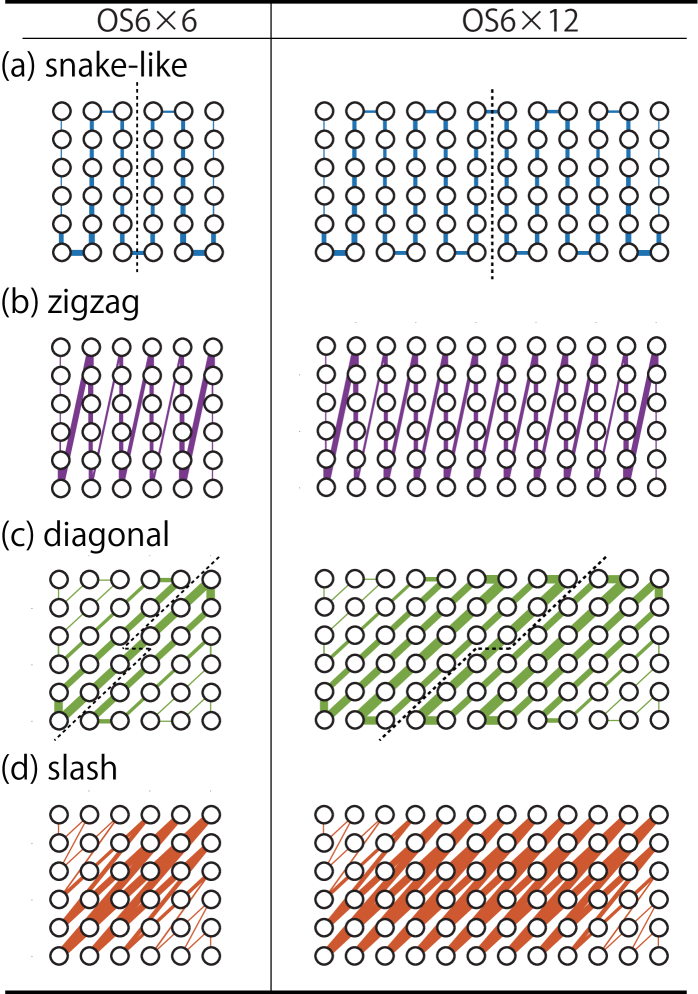
Figure 1: (Color online) Various MPO paths utilized in XTRG simulations that map the 2D lattices into quasi-1D system with long-range interactions, including (a) the snake-like, (b) zigzag, (c) diagonal, and (d) slash paths. The line width visualizes the low-temperature bond entanglement $S_{E}$ along the MPO obtained on the OS $6{\times}6$ and OS $6{\times}12$ lattices (at $T\simeq 0.06$), where we used a width of $w=(4S_{E}-11)\,\mathrm{pts}$, yet enforcing $w\geq 1$ for visibility.

II.2 Thermal Tensor Renormalization Group Methods

We employ thermal tensor renormalization group (TRG) methods, including XTRG and SETTN, to simulate the spin lattice models. In both approaches, the unnormalized density matrix $\rho(\beta)\equiv e^{-\beta H}$ of a finite-size 2D system is represented in terms of MPO in a quasi-1D setup. In XTRG, $\rho(\tau)$ at small inverse temperature $\tau$ is initialized through a Taylor expansion, i.e.,

$$\rho(\tau)\simeq\sum_{k=0}^{N_{c}}\tfrac{(-\tau)^{k}}{k!}H^{k},$$ (3)

with $N_{c}$ the cut-off order. The RG techniques required to construct efficient TTN representations of the initial $\rho(\tau)$ have been developed in the SETTN algorithms Chen et al. (2017).

After the initialization, we double the inverse temperature $\beta=2^{n}\cdot\tau$ of the density matrix $\rho_{n}$ in each iteration $n$ and thus cool down the system exponentially fast, i.e.,

$$\rho_{n+1}=\rho_{n}*\rho_{n},$$ (4)

where $*$ indicates MPO multiplication. XTRG turns out to be very efficient and accurate (compared to linearly decreasing the temperature, it yields smaller accumulated truncation errors due to significantly less truncation steps). It can be parallelized via a $z$-shift of the initial $\tau$, i.e., $\tau\rightarrow 2^{z}\tau$ with $z\in[0,1)$, to obtain fine-grained temperature resolution Chen et al. (2018). Overall, our approach is equivalent to the purification framework Feiguin and White (2005); Barthel et al. (2009); Li et al. (2011); Dong et al. (2017); Zwolak and Vidal (2004), and $T_{\mathrm{min}}\equiv 1/\beta_{\mathrm{max}}$ constitutes the lowest temperature reached.

Apart from providing a good initialization for small $\tau$, SETTN also provides an alternative way to determine $\rho(\beta)$ for simulations down to low temperatures, also operating on a logarithmic $\beta$ grid. To be specific, a point-wise Taylor expansion version of SETTN, proposed in Ref. Chen et al. (2018), is adopted in this work. It expands the thermal state

$$\rho(\beta)=\sum_{k=0}^{N_{c}}\tfrac{(-\beta+\beta_{n})^{k}}{k!}H^{k}\rho(\beta_{n}),$$ (5)

around a series of temperature points $\beta_{n}\to 2\beta_{n}$ starting at $\beta_{0}=\tau$, such that $\beta\in\{2\tau,4\tau,\ldots,2^{n}\tau\equiv\beta_{\mathrm{max}}/2\}$ for XTRG, as well as smaller $\beta$ steps in case of SETTN. Since truncation errors accumulate as $k$ increases in each $H^{k}\rho(\beta_{n})$ term of the series, this modified SETTN reduces the order $N_{c}$ required for the expansion thus improves the accuracy. Besides, the SETTN approach also benefits in efficiency from the logarithmic scales in temperature series $\{\beta_{n}\}$, since it reduces significantly the computational overhead in expansions.

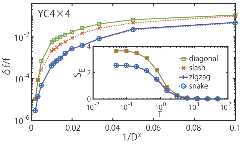
Figure 2: (Color online) Relative errors of free energy $f$ vs. $1/D^{*}$, $D^{*}$ the number of multiplets kept, for the YC $4{\times}4$ SLH at $T\simeq 0.06$, and the ED data are taken as the exact reference. Four mapping paths are compared, including the snake-like, slash, diagonal, and the zigzag one. The inset shows the maximum of $S_{E}$ over all MPO bonds, vs. $T$. One can observe that $S_{E}$ values coincide in the essentially equivalent snake-like and zigzag paths, and are significantly smaller compared to the diagonal and slash paths.

II.3 Thermal quantities and entanglement measurements

In this work, we are interested in various quantities, including the free energy $f$, internal energy $u$, specific heat $c_{V}$, and static magnetic structure factor $S({q})$, as well as MPO entanglement $S_{E}$ in the thermal states.

The free energy per site can be directly computed from the partition function,

$$f(\beta)=-\tfrac{1}{\beta N}\ln{\mathcal{Z}(\beta)},$$ (6)

where $\mathcal{Z}(\beta)=\rm{Tr}\bigl{[}\rho(\frac{\beta}{2})^{\dagger}\,\rho(\frac{\beta}{2})\bigr{]}$ is the partition function and $N$ is the total number of sites. The internal energy $u$ per site can be evaluated, in practice, in two different yet theoretically equivalent ways. A simple way is to compute the expectation value $u(\beta)$ directly by tracing the total Hamiltonian $H$ with density operators $\rho$ (referred to as scheme $a$),

$$u(\beta)=\tfrac{1}{N}\mathrm{Tr}\bigl{[}\rho(\tfrac{\beta}{2})^{\dagger}H\rho(\tfrac{\beta}{2})\bigr{]}.$$ (7a)

Since the MPO representations of the density matrices $$\rho H u f b$$ and Hamiltonian are available in XTRG and SETTN simulations, Eq. (7a) can be calculated conveniently via tensor contractions. Alternatively, one can also compute the internal energy by taking derivatives of free energy (referred to as scheme ),

$$u(\beta)=\tfrac{1}{N}\tfrac{\partial(f\beta)}{\partial\beta}=\tfrac{1}{N\beta}\tfrac{\partial(f\beta)}{\partial\ln{\beta}},$$ (7b)

where the last derivative is a natural choice when $\beta$ is chosen on a logarithmic grid. The specific heat $c_{V}$ is given by the derivative of the internal energy,

$$c_{V}=\tfrac{\partial u}{\partial T}=-{\beta}\tfrac{\partial u}{\partial\ln{\beta}},$$ (8)

again with preference to taking the derivative with respect to the logarithmic temperature scale, as shown in the last term.

In order to understand the spin structure at finite $T$, e.g., to probe the incipient order and estimate the spontaneous magnetization in the SLH model, we compute the static spin structure factor $S({q})$ at finite temperature, defined as

$$S(q)=\sum_{j}e^{-iq\cdot r_{ij}}\langle S_{i}\cdot S_{j}\rangle_{T},$$ (9)

where $r_{ij}\equiv r_{j}-r_{i}$ refers to the distance between lattice site $i$ and $j$. Dealing with finite system sizes, we fix $i$ in the center of the system, whereas $j$ runs over the entire lattice.

By choosing $q$ in the vicinity of the ordering wave vector $q_{0}=M\equiv(\pi,\pi)$ [cf. Fig. 6(e)], one has $S(q)=S(q_{0})/[1+\xi^{2}(q-q_{0})^{2}]$ (Ornstein-Zernike form), and thus $\xi^{2}\cong\bigl{.}\tfrac{-1}{2S({q})}\tfrac{\partial^{2}S({q})}{\partial{q}^{2}}\bigr{|}_{{q}={q}_{0}}$, from which it follows Elstner et al. (1993)

$$\xi^{2}(T)=\tfrac{c^{2}_{{q}_{0}}}{2S({q}_{0})}\sum_{j}{r}_{ij}^{2}\,e^{-\text{i}{q}_{0}\cdot{r}_{ij}}\,\langle{S}_{i}\cdot{S}_{j}\rangle_{T}\text{ ,}$$ (10)

where the constant $c^{2}_{{q}_{0}}\equiv\langle\cos^{2}\alpha_{ij}\rangle=1/2$ accounts for an angular average, with $\alpha_{ij}$ the angle in between ${q}_{0}$ and ${r}_{ij}$.

We also investigate the MPO entanglement, which offers direct information on the numerical efficiency of our thermal RG simulations. In XTRG, the MPO density matrix can be regarded as a purified superstate $|\tilde{\Psi}_{\beta/2}\rangle\hat{=}\rho(\beta/2)$, which is unnormalized, hence the tilde. By definition then, the partition function can be calculated as $\mathcal{Z}(\beta)=\langle\tilde{\Psi}_{\beta/2}|\tilde{\Psi}_{\beta/2}\rangle$. This thermofield double purification employs identical ancillary and physical state spaces. It is then useful to introduce a formal entanglement measure, $S_{E}$, for the MPO. For this, we divide the normalized super-vector $|\Psi_{\beta/2}\rangle$ (hence no tilde) – represented now as an effective matrix product state (MPS) with twice as many, paired up local degrees of freedom – into two blocks w.r.t. some specified bond, and compute the standard MPS block-entanglement (von Neumann) entropy $S_{E}$ Schollwöck (2011); Chen et al. (2018). The latter is a measure of both quantum entanglement and classical correlations. As such, $S_{E}$ is a quantity of practical importance in our thermal RG simulations, since the bond dimension $D\sim e^{S_{E}}$ quantifies the required computational resource for an accurate description of the thermal states.

In conformal quantum critical chains, the MPO entanglement $S_{E}$ scales logarithmically vs. $\beta$, as derived from conformal field theory Dubail (2017) and confirmed in large-scale numerics Prosen and Pižorn (2007); Barthel ; Chen et al. (2018). The temperature dependence of $S_{E}$ strongly depends on the underlying physics. In the following, it will be analyzed in detail in this regard for the SLH, which has low-energy gapless modes due to the spontaneous SU(2) symmetry breaking, as well as in the QIM, which undergoes a finite-$T$ phase transition.

In our XTRG simulations of the SLH, finally, we also fully exploit the global SU(2) symmetry in the MPO based on the QSpace tensor library Weichselbaum (2012). In these SU(2) symmetric calculations, a state-based description of any state space or index is replaced in favor of a description in terms of multiplets. Specifically, $D$ states on the geometric MPO bonds are equivalently reduced to $D^{\ast}\simeq D/4$ multiplets, with $D^{\ast}$ the tuning parameter. Given the numerical cost for XTRG being $\mathcal{O}(D^{4})$ Chen et al. (2018), the implementation of non-Abelian symmetry in XTRG therefore greatly improves its computational efficiency. Conversely, this allows us to reach lower temperatures.

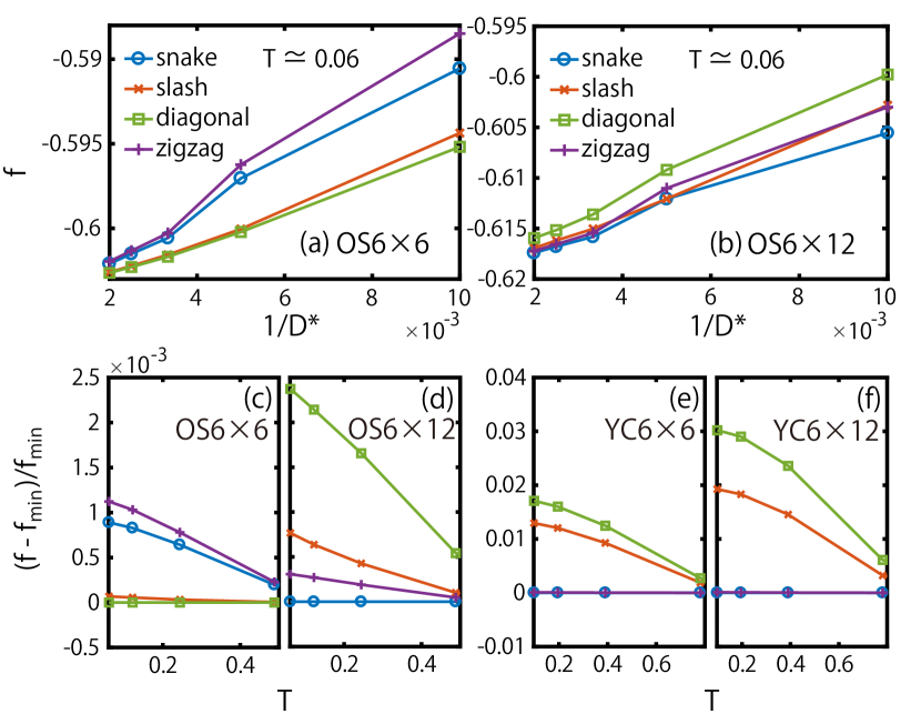
Figure 3: (Color online) The free energy $f$ of SLH on the (a) OS $6{\times}6$ and (b) OS $6{\times}12$ lattices at $T\simeq 0.06$, obtained for the four different MPO paths in Fig. 1 by retaining $D^{\ast}=100$ to $500$ multiplets in all cases. (c, d, e, f) show comparisons of the free energy $f$ vs. $T$ for all paths using $D^{\ast}=500$ for OS (c,d) and YC (e,f). Here $f_{\mathrm{min}}(T)$ represents the minimal value amongst all four paths at any given $T$.

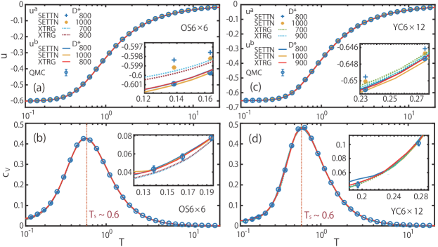
Figure 4: (Color online) Internal energy $u$ and specific heat $c_{V}$ for (a,b) OS $6{\times}6$, and (c,d) YC $6{\times}12$ SLH systems. The insets zoom into the low-$T$ data, where the SETTN and XTRG data for various $D^{*}$ are shown to agree excellently with QMC. In the legends, $u^{a}$ and $u^{b}$ refer to the two schemes in Eqs. 7 (a) and (b), respectively. The specific heat $c_{V}$ in the lower panels is obtained from $u$ using Eq. (8). The vertical dashed line represents the temperature scale $T_{S}\sim 0.6$ in SLH.

III Various MPO paths in thermal renormalization group simulations

Since our MPO-based RG methods map the 2D lattice models into a quasi-1D setup, the sites of the lattice must be brought into a serial order. This introduces a ‘mapping path’ throughout the lattice, the specific choice of which clearly includes some arbitrariness. This has already been discussed before in a similar context in DMRG simulations Xiang et al. (2001). There the authors considered ordering the sites along the diagonal direction [cf. Fig. 1(c)], made some comparisons to the conventional snake-like path [cf. Fig. 1(a)], and arrived at a conclusion that the diagonal path gets better, i.e., lower variational energy, when the same number of bond states is retained. Here we perform a similar analysis for our thermal simulations. For comparison, we include a few more conventional paths in our thermal RG simulations, with the expectation to recover the observations made in previous DMRG study mentioned above for the same geometry.

To be specific, in Fig. 1 we compare four simple choices of paths: the snake-like (blue color), slash (orange), diagonal (green), and the zigzag one (purple). We perform XTRG calculations down to low temperatures for these MPO paths on systems including $4\times 4$ (YC), $6\times 6$, and $6\times 12$ (both OS and YC) geometries. Throughout this section (as well as in App. B), the same color code is adopted in all related plots, e.g., Figs. 1,2,3 as well as Fig. A2.

Firstly, we benchmark the SLH on a small YC $4{\times}4$ lattice also accessible by exact diagonalization (ED), by checking the relative error of the free energy $f$ at a low temperature ($T\simeq 0.06$) in Fig. 2. Clearly, $\delta f/f$ improves continuously with increasing $D^{*}$, down to $\sim 10^{-5}$ for $D^{*}=500$ retained bond multiplets. Overall, we conclude from Fig. 2, that the snake-like and the zigzag paths turn out to be optimal amongst all four choices.

However, the conclusion reached depends on the system size, specifically so for smaller ones. In Figs. 3(a,b), we compare four MPO paths on the larger OS $6{\times}6$ and OS $6{\times}12$ systems, where $f$ is compared at $T\simeq 0.06$. Although ED data is no longer available to compare to, the XTRG results for $f$ are variational. Therefore a lower value of $f$ still unambiguously serves as a useful criterion for accuracy. In Figs. 3(a,c), for the OS $6{\times}6$ system, we find the diagonal, as well as the slash path, leads to a lower, thus better, $f$, by a relative difference $\lesssim 0.1\%$. This is in agreement with the observation in Ref. Xiang et al. (2001), where they also find that the diagonal path produces energetically better results.

However, the situation quickly reverses again for larger systems, and in particular also for the cylindrical geometries. On the longer OS $6{\times}12$ lattice [Figs. 3(b,d)], the snake-like path produces lower results for $f$, closely followed by the zig-zag, while the diagonal one now leads to highest $f$ amongst all four choices, still with relative differences $\lesssim 0.2\%$. For the YC geometries, as shown in Figs. 3(e,f), the snake-like path is again found to be the optimal choice, and the diagnal path the least favorable one, with $f$ now a few percent larger at our lowest temperatures. Conversely, the snake-like and the zigzag paths show strong consistency within $10^{-4}$ relative difference.

To shed some light on understanding the performance of various mapping paths, we show the landscape of thermal entanglement $S_{E}$ vs. MPO bond indices in Fig. 1, where the bond thickness represents the “strength” of entanglement. From Fig. 1, as well as Fig. A2, one can see that the snake-like and the zigzag path have a comparatively small entanglement throughout their paths. To be specific, for the snake-like and zigzag paths, the bond entanglement distribution is rather uniform (except for few bonds near both ends). By contrast, for the slash and diagonal paths, there exist numerous thick lines in the bulk, leading to overall larger truncation errors (see App. B for detailed data) and thus higher free energy results.

One can understand the entanglement “strength”, as well as required bond dimensions, on a given MPO bond in a somewhat intuitive way: since we divide the system into two halves by cutting only one MPO bond, it is natural to associate the required bond dimension to the smallest possible number of coupling bonds (lattice links) intersected by that specific cutting line (see, e.g., dashed lines in Fig. 1). For OS $6{\times}6$ (left column of Fig. 1), in the snake-like and zigzag paths, the typical bipartition line cuts 6 interaction links, while for the diagonal and slash cases, this number is 10. Note also that when the dashed cutting line has a corner, it can introduce some additional constant contribution to the MPO entanglement, which helps understand the specific location of “thick” bonds in various paths in Fig. 1. While for OS $6{\times}6$ one may argue, that entanglement only concentrates on the narrow (anti-)diagonal and hence may be beneficial, for more general geometries, say, long OS $6{\times}12$, shown in the right column of Fig. 1 (as well as in cylindrical geometries, not shown), the snake-like or zigzag path clearly constitutes a better choice.

To summarize, except for OS $6{\times}6$ where the diagonal-path has a slightly better performance, indeed, in agreement with previous DMRG results Xiang et al. (2001), for larger systems the snake-like or zigzag paths are generally expected to lead to lower free energy. Overall, we observe that from a computational and accuracy point of view, zigzag and snake-like paths are essentially equivalent and, in certain ways, so are slash to diagonal paths. As expected and shown explicitly in Fig. 3, the accuracy for all paths increases with increasing $D^{\ast}$. Nevertheless, this barely changes the preference on a given path. Based on these observations and arguments, the snake-like path is adopted in our practical simulations throughout the rest part of the paper.

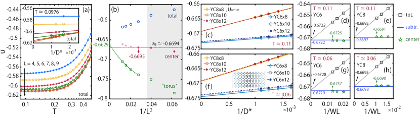
Figure 5: (Color online) (a) Internal energy $u$ on the OS $L{\times}L$ lattices up to $L=9$ calculated by XTRG keeping up to $D^{*}=1000$ multiplets. The data are obtained in three different ways (total, central, and “torus”) as described in the main text, with total shown in main panel (a), and finite size scaling of the extrapolated data vs. $1/L^{2}$ shown in panel (b). In order to reduce the finite $D^{*}$ effects, we extrapolate the internal energy $u$ to $1/D^{*}=0$, as seen in the inset of (a). In (b) we collect the low-temperature ($T\simeq 0.1$) data extrapolated in (a) $1/D^{\ast}\to 0$ and analyze it here vs. $1/L^{2}\to 0$. For “torus”, we extrapolate the four largest system sizes (i.e., data in gray shaded area was excluded), to the thermodynamic limit, via a second-order polynomial fitting vs. $1/L^{2}$. The horizontal dashed line represents the ground state energy $u_{g}\simeq-0.6694$ from QMC Sandvik (2010). For comparison, (c-h) analyses the internal energy $u$ of SLH on YC $6{\times}L$ and YC $8{\times}L$ cylinders of lengths $L=8,10,12$. Exemplary extrapolations of $u_{\mathrm{center}}$ vs. $1/D^{\ast}\to 0$ are shown in panels (c) and (f) for $T\simeq 0.11$ and $0.06$, respectively, where $u_{\mathrm{center}}$ is evaluated via a weighted average around the center as illustrated in the inset of (f) (see main text for more details). The results at $1/D^{\ast}\to 0$ are collected vs. $1/WL$ in panels (d, e, g, h) (green stars). There they are also compared to similarly extrapolated data for $u_{\mathrm{tot}}$ (black squares), as well as to $u_{\rm{subtr}}$ (blue horizontal line) obtained by subtracting the length $L=8$ from the $L^{\prime}=12$ cylinder. With $u_{\mathrm{tot}}$ also extrapolated to $1/WL\to 0$, we find good agreement across our data towards the thermodynamic limit.

IV Square-Lattice Heisenberg Model

In this and the next section we present our main thermodynamic results for the SLH and the QIM, respectively. We benchmark them against QMC data generated by the looper algorithm from ALPS Bauer et al. (2011).

IV.1 Internal energy and specific heat

In Fig. 4, we present the results for the internal energy $u$ as well as specific heat $c_{V}$, where we have employed both XTRG and SETTN to simulate the SLH on two lattices, OS $6{\times}6$ and YC $6{\times}12$. We have also compared the two schemes for computing $u$ and their derived $c_{V}$ in Fig. 4: (a) as expectation values by tracing the Hamiltonian [cf. Eq. (7a)], or (b) by taking the derivative of free energy [cf. Eq. (7b)].

The internal energy results $u$ obtained from both schemes agree very well with the QMC data, as shown in Figs. 4(a,c). By strongly zooming in into the low-$T$ regime, nevertheless, it turns out that scheme $b$ results in slightly better accuracy, in both XTRG and SETTN simulations. Still given the same bond dimension, within scheme $a$, XTRG data demonstrates better accuracy than those of SETTN. This observation is consistent with the general observation that XTRG produces more accurate results due to the much smaller number of evolution and thus truncation steps Chen et al. (2018) for the density matrix $\rho(\beta/2)$.

The slight difference between the two schemes $a$ and $b$ is arguably due to truncation: truncation is biased to keep the strongest weights in $\rho$, such that $\mathcal{Z}(\beta)=\mathrm{Tr}[\rho(\beta/2)^{\dagger}\rho(\beta/2)]$ is optimally represented, hence also $f\sim-\frac{1}{\beta}\ln\mathcal{Z}$, and thus also its derivative $u$, i.e., as in scheme $b$. Conversely, by computing $u$ directly as in scheme $a$ via the expection value $\mathrm{Tr}\bigl{(}\rho^{\dagger}H\rho\bigr{)}$, this is not necessarily guaranteed to be optimally represented in the presence of truncation. This heuristically explains the slightly better performance of scheme $b$.

We also compare the specific heat $c_{V}$ derived from the respective internal energy data obtained from both XTRG and SETTN simulations in schemes $a$ and $b$. The results are shown in Figs. 4(b,d), with the same conclusion as for the internal energy $u$: scheme $b$ leads to a slightly better numerical performance for both RG methods. The peak position for $c_{V}$ allows us to read off a characteristic crossover temperature $T_{s}$ for the SLH, separating the low-temperature regime showing incipient long-range order from a high-temperature regime without such order (as discussed in more details below).

To scale the results to the thermodynamic limit, we show the internal energy $u$ of SLH on OS $L{\times}L$ lattices with $L=4$ to 9 in Fig. 5(a). We collect the energy values calculated by scheme $b$ [Eq. (7b)] at our lowest reliable temperature $T\simeq 0.1$, which already provides a very good estimate of ground state energy Okabe and Kikuchi (1988). With the $u$ data well converged vs. $T$ on the finite-size clusters, we extrapolate the energy results to $1/D^{\ast}\to 0$ as shown in the inset of Fig. 5(a). Three slightly different ways of extrapolating the ground state energy towards the thermodynamic limit $1/L^{2}\to 0$ are presented in Fig. 5(b): total (blue circles) is obtained by dividing the total energy by the number of sites $N=L^{2}$, torus (green squares) to be defined below, and center (maroon asterisks). The latter is obtained from an smooth average emphasizing center sites, computed as $u_{\mathrm{center}}\equiv\tfrac{1}{\sum_{i}{w_{i}}}\sum_{i}{w_{i}u_{i}}$, where $u_{i}$ is the energy per site which equals half the plain sum of nearest-neighbor bond energies around the site $i$, and the weighting factors are taken as $w_{i\equiv(i_{x},i_{y})}=\sin^{2}\bigl{(}\frac{i_{x}-1}{L-1}\pi\bigr{)}\sin^{2}\bigl{(}\frac{i_{y}-1}{L-1}\pi\bigr{)}$, with $i_{x},i_{y}\in[1,L]$. They are maximal in the center and smoothly diminish towards the open boundary where they vanish quadratically, hence suppressing the influence of the open boundary. This center data converges fast vs. $1/L$. For $L=6$ it already equals $-0.6695$ in excellent agreement with the QMC result $u_{g}\simeq-0.6694$ (see, e.g., Ref. Sandvik (2010)). However, for our largest system sizes, $L\gtrsim 7$, the bond energy distribution starts getting weakly affected by our limited bond dimension $D^{*}$, e.g., see extrapolation in $1/D^{\ast}$ in the inset of Fig. 5(a). Thus $u_{\mathrm{center}}$ starts to drift away from the plateau approximately reached for $L\sim 6$ due to an increased error in the extrapolation $1/D^{\ast}\to 0$. A similar behavior is likely also observed for the ‘total’ data for the largest system sizes.

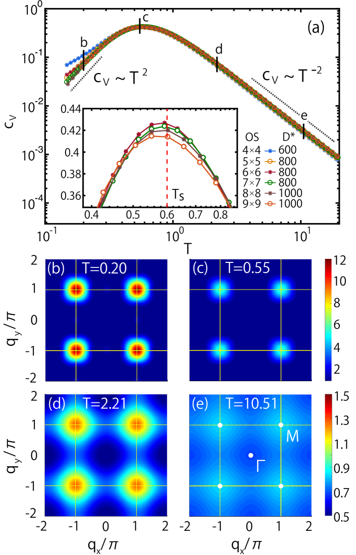
Figure 6: (Color online) (a) SLH specific heat $c_{V}$ on the OS $L{\times}L$ lattices on log-log scale to emphasize the algebraic behavior at high and low temperature, obtaining, $c_{V}\sim T^{-2}$ and $\sim T^{2}$, respectively (see dashed lines as guide to the eye). The inset zooms into the peak at intermediate temperatures around $T_{S}\sim 0.6$. Panels (b-e) show the static spin structure factors $S({q})$ on OS $9{\times}9$ at $T\simeq 0.20$, $0.55$, $2.21$, and $10.51$, respectively. The grid lines demarcate the Brillouin zone, where the white dots in (e) indicate specific high-symmetry points therein.

To further confirm the energy extrapolation, a fictitious torus (green squares) is introduced, which also incorporates a weighted average $u_{\mathrm{torus}}=\tfrac{1}{N}\sum_{i}w^{\prime}_{i}u_{i}$. Here the weights $w^{\prime}_{i}$, defined as

$$w^{\prime}_{i}=\left\{\begin{aligned} 1\text{,}&\,\,&&{i\in\text{bulk}}\\ {4}/{3}\text{,}&\,\,&&{i\in\text{edge}}\\ 2\text{,}&\,\,&&{i\in\text{corner }}\end{aligned}\right.$$

reflect the fact that boundary sites have missing bonds w.r.t. a fictitious torus, i.e., a corner site has two bonds missing (so we multiply the site energy by a factor of $w^{\prime}_{i}=2$) and an edge site one bond (thus $w^{\prime}_{i}=4/3$). In a sense we are estimating the energy values on a “torus”, by adding the missing bonds of a given boundary site whose energies replicate existing nearest-neighor bonds. This somewhat overestimates the energies of the boundary sites, such that the ground state energy converges from below now, as seen in Fig. 5(b). We extrapolate this data for the “torus” only including the data points of $L\geq 6$) to the thermodynamic limit via a polynomial fitting. From this we obtain $u_{g}^{*}\simeq-0.6629$, which is slightly above the QMC result.

For comparison, we also simulate YC geometries of widths $W{=}6$ and $8$ at two temperatures $T\simeq 0.11$ and $0.06$, with their internal energy $u$ analyzed in Figs. 5(c-h). As seen in Figs. 5(c,f) similar to the inset in Fig. 5(a), the convergence of $u_{\mathrm{center}}$ exhibits a nearly linear behavior vs. $1/D^{\ast}$ and can thus be well extrapolated to $1/D^{\ast}=0$. The extrapolation over $1/D^{*}$ may also be replaced by an extrapolation of the truncation error, i.e., the discarded weight $\delta\rho\to 0$. We show in App. C for the case of YC6 and YC8 at $T\simeq 0.06$ that both extrapolations agree well at low temperatures.

Similar to Fig. 5(b) we compare the internal energy in three different ways in Figs. 5(d,e,g,h) (again all extrapolated to $1/D^{\ast}\to 0$), except that the earlier fictitious torus is replaced by a subtracted data set for $u_{\rm{subtr}}$ (horizontal lines) which is obtained from the difference in $u_{\mathrm{tot}}$ between $L=8$ and $L^{\prime}=12$ cylinders, divided by $(L^{\prime}-L)\cdot W$ sites. Also for the case of cylinders, $u_{\mathrm{center}}$ is the energy per site weighted by a factor $\sin^{2}(\frac{i_{x}-1}{L-1}\pi)$ that is uniform around the cylinder, i.e., independent of $i_{y}$, with $i_{x}\in[1,L]$ indexing columns along the cylinder. The weights are illustrated in the inset of Fig. 5(f), where the intensity gradually decreases from the center to both ends. Besides this “smooth” average, we have also tried the computation of $u_{\mathrm{tot}}$ sharply restricted within the 1$\sim$2 central columns of the cylinder, yielding slightly less systematic results. Overall, the results of all three schemes are in good agreement with each other, as well as with the QMC data $u_{g}\simeq-0.6694$ Sandvik (2010). For example, in the case of YC8 at $T\simeq 0.06$, $u_{\mathrm{tot}}=-0.6695$, $u_{\mathrm{subtr}}=-0.6698$, and $u_{\mathrm{center}}=-0.6690$, leading to an accurate estimate of ground state energy $u_{g}^{*}=-0.6694(4)$.

The derivative of the internal energy yields the specific heat $c_{V}$ [cf. Eq. (8)], shown for the SLH in Fig. 6(a) on OS $L{\times}L$ lattices up to $L=9$. We observe a well-pronounced single peak located at $T_{S}\sim 0.6$. Given that is largely independent of system size (see inset), this data already reflects the thermodynamic limit (even though simulating finite system sizes!). This observation is consistent with the scenario that there is no phase transition in SLH at finite $T$ and, consequently, that $T_{S}$ represents a crossover scale of thermodynamic behavior.

IV.2 Static Structure Factor

Next, we explore the spin structure factor $S({q})$ at various temperatures. We select four temperatures corresponding to different regimes in the specific heat [see markers (b-e) in Fig. 6(a)], and show their $S({q})$ data in Figs. 6(b-e), respectively. High symmetry points in the Brillouin zone (BZ) including the central point $\Gamma=(0,0)$ and $M=(\pm\pi,\pm\pi)$ are indicated explicitly in Fig. 6(e). At low temperature $T\ll T_{S}$, there exists a clearly established incipient order, which gives rise to the sharp bright spots at the $M$ points. As $T$ increases, the system passes the cross-over scale $T\sim T_{S}$, at which stage the incipient order has already become significantly weakened, as shown in Fig. 6(c). As the temperature increases further, the originally bright spot at the $M$ points becomes ever weaker [Figs. 6(d,e), note also the altered color bar scale], until it is completely blurred out for temperatures $T>10$ [Fig. 6(e)].

Besides the bright $M$ points, the $S(q)$ contour shows nontrivial patterns near the crossover scale. We illustrate this on the example of an OS $9{\times}9$ SLH system in Fig. 7. It zooms in the low-intensity part of $S(q)$, showing salient patterns in stark difference between the high- and low-temperature regimes. At high temperature $T\simeq 12.5$ [Figs. 7(a,b)], there exists a clear-edged “diamond” shape surrounding the $M$ points. On the other hand, in the low-temperature regime, e.g. $T\simeq 0.2$ [Figs. 7(c,d)], the diamonds have significantly shrunk and rotated by $45^{\circ}$.

In order to get a better intuitive understanding, we employ two simple models, the independent dimer approximation (IDA) and the antiferromagnetic Ising (AFI) model. In IDA, we assume that a given site is in a singlet configuration with either one of its nearest-neighbor sites with probability $1/4$ for each, and no further longer-range correlations. This yields the spin structure factor

$$S_{D}(q_{x},q_{y})=\tfrac{3}{8}\left(2-\cos q_{x}-\cos q_{y}\right),$$ (11)

which describes short-range correlation (typically at high $T$). On the other hand, the AFI spin structure factor $S_{I}$ is evaluated from spin correlations of classically ordered antiferromagnet configurations on an OS $5{\times}5$ lattice, to capture the essential feature in the spin-spin correlation at low temperatures.

Indeed, at high temperatures we find that a fit of the form $S(q)=aS_{D}+c$ based on IDA with parameters $a=0.08$ and $c=0.69$ [as shown in Fig. 7(b)] provides a good description of the XTRG data in Fig. 7(a). From this we conclude that at high temperatures $T\gg T_{S}$, IDA can reproduce the diamond pattern and capture very well the residual magnetic correlations in the system. Note that, by definition, the $q$-independent term in $S(q)$ must be equal to $\mathbf{S}^{2}=3/4$, hence $\tfrac{3}{4}a+c\simeq 0.75$ [cf. Eq. (11)] with $a\ll 1$ at large $T$.

At low temperatures, we employ the AFI correlation introduced above to describe the developed incipient order, together with the dimer correlations taking care of the short-range fluctuations, again under IDA assumption. The structure factor is therefore then fitted using the combination $S({q})=aS_{D}+bS_{I}+c$, where we find that $a=4.5$, $b=25$, and $c=-2.7$ well resembles the XTRG $S({q})$ data (larger values of $a$ and $b$ suggest longer-range correlations as expected, indeed), including even the very subtle details of the four-leaf shape.

For pure long-range AFI correlations, the $q_{x}$ and $q_{y}$ components decouple in the structure factor into a product of independent terms, such that $S(q)$ develops square-like peaks around the $M$ points that are aligned with the BZ. At high temperatures, instead, the lines are aligned with the smaller magnetic BZ boundary, given that the real-space lattice unit cell is enlarged. This explains why the diamond pattern in Figs. 7(a-b) rotates into aligned square like peaks in Figs. 7(c-d). In this sense, the inclusion of $S_{D}$, i.e., short-range correlations, is important to allow four little “leaves” to appear (which may disappear in the thermodynamic limit, though). We believe, however, that the dominant features seen in the $S(q)$ contours in Fig. 7, indeed, encode important information on the spin structures in the system. Apart from the different brightness of $S(M)$, this feature constitutes another relevant distinction in $S(q)$ between the high- and low-temperature regimes. We expect that these salient patterns in $S(q)$ may find their experimental realizations in quantum simulators using cold atoms Mazurenko et al. (2017).

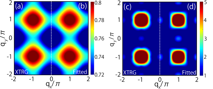
Figure 7: (Color online) The static spin structure factors $S({q})$ on the OS $9{\times}9$ lattice at (a) $T\simeq 12.5$ and (c) $T\simeq 0.2$, calculated by XTRG. Fittings using the antiferromagnetic Ising (AFI) model and independent dimer approximation (IDA) (see main text) are presented at the right half of each panel [(b) and (d)], which enjoy excellent agreement with XTRG data on the left half of each panel [(a) and (c), respectively].

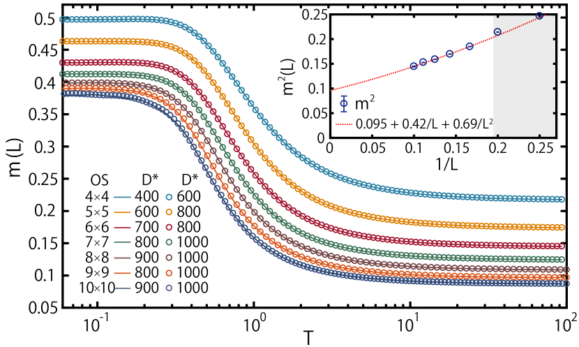
Figure 8: (Color online) The finite-size analysis of spontaneous magnetization $m(L)\equiv\sqrt{S(M)/L^{2}}$ of the SLH on the OS $L{\times}L$ lattices up to $L=10$. In the inset, we collect $m^{2}(L)$ data at $T=0.1$ where convergence vs. $T$ is reached, and extrapolate it to the thermodynamic limit $1/L\to 0$ using a parabolic fit. The data in the gray shaded area was excluded from this fit. From this we estimate the value for the thermodynamic limit $m_{S}^{*}\simeq 0.30(1)$, in good agreement with the literature, $m_{S}\simeq 0.3070(2)$ Sandvik (1997).

IV.3 Spontaneous Magnetization and Incipient Order at $T>0$

From the spin structure factor $S({q})$ at the ordering point $q_{0}\equiv M$, we can estimate the spontaneous magnetization $m_{S}$. To be specific, we employ the low-temperature finite-size spontaneous magnetization $m(L)=\sqrt{S(M)/L^{2}}$ on the OS $L{\times}L$ as an estimate, which is shown as a function of $T$ in Fig. 8. We find for all systems explored, including our largest system at $L=10$, that $m(L)$ has essentially saturated at low temperatures $T\lesssim 0.1$. We then collect the converged values of $m(L)$, plot $m^{2}(L)$ vs. $1/L$ Sandvik (1997) in the inset of Fig. 8. A quadratic fit in $1/L$ then yields the estimate $m_{S}^{*}\simeq 0.30(1)$. This XTRG result is in good agreement with the QMC value $m_{S}\simeq 0.3070(2)$ Sandvik (1997).

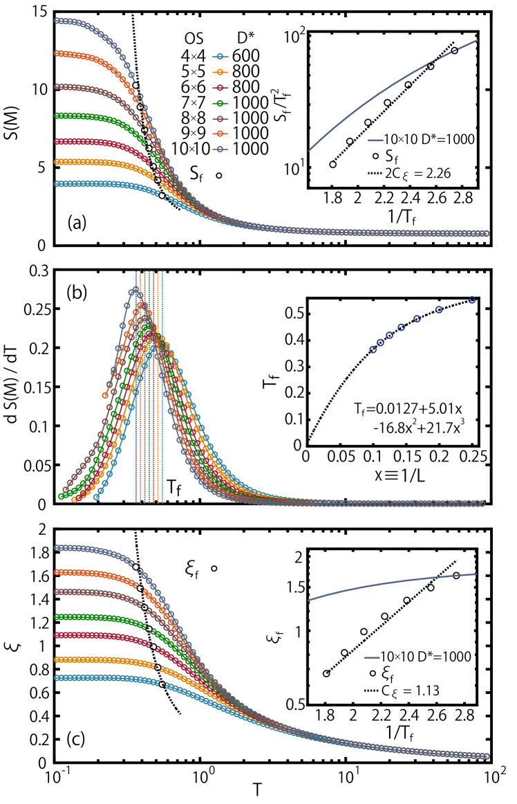
Figure 9: (Color online) (a) Static structure factor $S(M)$ vs. $T$ (same data as in Fig. 8). Its derivative in (b) has a maximum which defines a specific temperature $T_{f}$ at which finite size effects become significant. The inset in (a) then analyzes $S_{f}/T_{f}^{2}$ vs. $1/T_{f}$. The inset in (b) shows that $T_{f}$ extrapolates to $0$ in the thermodynamic limit, via a cubic fit as shown based on the data with $L\geq 4$. (c) Correlation length $\xi$ vs. $T$. The results for $S(M)$ and $\xi$ evaluated at $T_{f}$, are marked by black circles in the main panels (a,c), respectively. The data is collected and analyzed in the respective insets vs. $1/T_{f}$ which, overall, shows good agreement with RC predictions (dashed line). For comparison, the insets in (a,c) also plot the data for S(M) and $\xi$ vs. $1/T$ for the largest system size.

IV.4 Renormalized Classical Behaviors

At low temperatures, $T\ll T_{S}$, the SLH enters the universal RC regime Chakravarty et al. (1988, 1989). As observed in large-scale QMC simulations Beard et al. (1998); Kim and Troyer (1998), as well as in neutron scattering experiments Chakravarty et al. (1988), the incipient order and RC scalings have been quantitatively confirmed. To be specific, the correlation length $\xi$ diverges exponentially with decreasing $T$ as

$$\xi(T)=A_{\xi}\,e^{C_{\xi}/T}[1+\mathcal{O}(T)],$$ (12)

and the structure factor $S({q})$ also diverges at the ordering point as

$$S(M)=A_{S}\,T^{2}e^{2C_{\xi}/T}[1+\mathcal{O}(T)],$$ (13)

where $A_{\xi}$, $A_{S}$, and $C_{\xi}=2\pi\rho_{s}$ are constants, with $\rho_{s}$ the spin stiffness Elstner et al. (1994).

The universal RC scalings in Eqs. (12, 13) are strictly valid only in the thermodynamic limit $L\to\infty$. In our OS $L{\times}L$ XTRG simulations, we only have finite-size thermal data up to $L=10$, such that below (some) low temperature our finite-size XTRG data necessarily will deviate from the exponential scalings. This occurs once the thermal correlation length reaches system size. It coincides with the temperature where the structure factor $S(M)$ starts to saturate which was already clearly observed in Fig. 8 [replotted in Fig. 9(a) directly as $S(M)$ itself].

We may also use this as a criterion to define the (maximal) thermal correlation length that fits into a given finite system. Based on this then, we may analyze the onset of RC behavior from our finite-size data. We start by estimating a temperature $T_{f}$ below which the finite (f) size effects become prominent. We define it as the temperature at which the derivative $dS(M)/dT$ shows a maximum, as indicated by the vertical dashed lines in Fig. 9(b). Being due to finite size effects, a polynomial fitting vs. $1/L$, as shown in the inset of Fig. 9(b), shows that $T_{f}\to 0$ for $1/L\to 0$, as expected. Next we collect $S(M)$ evaluated at $T_{f}$ (denoted as $S_{f}$) from various OS $L{\times}L$ systems. A semilog plot, shown in the inset of Fig. 9(a), shows that this approximately supports an exponentially diverging behavior, indeed. This notably differs from the data for $S(M)_{T}$ simply plotted vs. $1/T$ for the largest system size, also shown for comparison (blue line). While for large temperatures (smaller $1/T$) the slope on the log-plot approximately coincides with the earlier $S_{f}$ analysis, it shows clear deviations due to finite size at lower temperatures (larger $1/T$). This is in contrast to the analysis vs. $1/T_{f}$ which was designed to largely eliminate finite size effects. We have compared the $S_{f}$ vs. $T_{f}$ curve to the standard RC formula Eq. (13) with $C_{\xi}=2\pi\rho_{s}\simeq 1.13$ Elstner et al. (1994), as indicated by the dashed lines in both the main panel and the inset of Fig. 9(a). The remarkable agreement strongly suggests that the RC behavior can be uncovered in the finite-size data via a careful analysis.

Similar to the analysis of the structure factor $S_{f}$ at the $M$ point, one can compute the (maximal) correlation length $\xi_{f}\equiv\xi(T_{f})$ as shown in Fig. 9(c). The resulting RC behavior of $\xi_{f}$ vs. $1/T_{f}$ is shown in the inset. In the present case, it is well-fitted by Eq. (12), thus again supporting RC scaling.

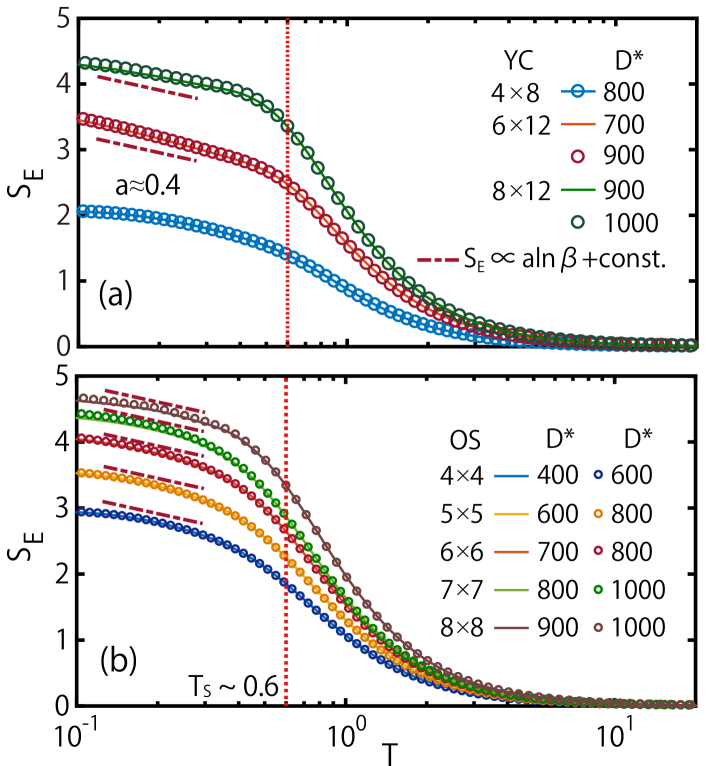
Figure 10: (Color online) MPO entanglement entropy $S_{E}$ on (a) cylinders YC $4{\times}8$, YC $6{\times}12$, and YC $8{\times}12$, and (b) OS $L{\times}L$ with $L=4$ to $8$. The tilted dashed lines in both (a) and (b) represent $S_{E}\propto a\ln{\beta}+\mathrm{const.}$, with slope $a\simeq 0.4$ (see dashed guides on top of the curves). The vertical dotted line represents the temperature scale $T_{S}\sim 0.6$ [e.g. see Fig. 6(a)].

IV.5 Entanglement Scaling

Low-temperature logarithmic scalings in the entanglement entropy $S_{E}$ have been observed in a number of quantum systems with gapless excitations. Near the conformal critical points in 1D quantum systems, the entanglement entropy scales like $S_{E}=a\ln{\beta}+\mathrm{const.}$, with $a$ proportional to the conformal central charge Chen et al. (2018, 2019); Barthel ; Dubail (2017); Prosen and Pižorn (2007); Žnidarič et al. (2008). For 2D quantum systems with gapless Goldstone modes, e.g., the triangular lattice Heisenberg antiferromagnet Chen et al. (2019), logarithmic entanglement also appears and can be related to a tower of states due to the ground-state SU(2) symmetry breaking. On intuitive grounds, one may expect a slowdown of the entanglement entropy at low temperatures, bearing in mind that the classical AF ground state is a product state.

In Fig. 10, we plot the thermal entanglement entropy $S_{E}$ vs. $T$, for YC and OS geometries. In Fig. 10(a), despite a rapid (algebraic) decrease at high temperatures, $S_{E}$ “crosses over” into a logarithmic behavior in the low-temperature regime around $T<T_{S}$, with an estimated slope of $a\simeq 0.4$ approximately independent of the system width (note that, in contrast, the temperature independent offset in $S_{E}$ is roughly proportional to the system width). The transition temperature is consistent with the crossover scale $T_{S}\sim 0.6$ that had been identified from the peak position in the specific heat, e.g., see Fig. 4 or Fig. 6(a). Hence, from Fig. 10 we find that the incipient AF order for $T_{S}\sim 0.6$ is directly linked to a weak logarithmic scaling of the entanglement entropy vs. $T$. For the OS systems in Fig. 10(b) we find stronger finite-size effects with an onset of saturation at our smallest temperatures, qualitatively similar to what is already also visible for our smallest OS $4{\times}4$. Still also for the OS systems, we find approximately the same logarithmic scaling of $S_{E}$ with the same slope as for the cylinders in Fig. 10(a) for $T<T_{S}$.

V Magnetic Phase Transition in the Quantum Ising Model

In this section we study the QIM as an exemplary minimal model system that exhibits a finite temperature phase transition. It thus constitutes a very meaningful benchmark for XTRG. While not explicitly analyzed here, at $T=0$, the square-lattice QIM also possesses a QPT at a critical field $h_{c}=1.52219(1)$, between the paramagnetic and ferromagnetic phases Blöte and Deng (2002); Orús and Vidal (2009); Orús (2012). Finite-temperature properties of the QIM have also been explored by TPO simulations Czarnik et al. (2012); Czarnik and Dziarmaga (2015) in the thermodynamic limit.

We show XTRG results for the QIM [Eq. (2)] in Figs. 11–13 for YC geometries up to width $W=8$ with a fixed aspect ratio $L/W=2$, as well as OS $L{\times}L$ with $L$ up to 10. Due to the transverse field, the system only possesses $\mathbb{Z}_{2}$ symmetry. We focus on the fixed value $h_{x}=\frac{2}{3}h_{c}$ of the transverse field where the model exhibits a thermal transition at the critical temperature $T_{c}\simeq 0.4239$ Czarnik and Dziarmaga (2015). There we analyze various thermal quantities of interest, including the specific heat $c_{V}$, Binder ratio $U_{4}$, and the MPO entanglement $S_{E}$. We exploit them to study the finite-temperature phase transition. A detailed comparison to QMC is performed, whenever the latter is available.

V.1 Specific heat

The specific heat $c_{V}$ from XTRG is compared to standard QMC data on YC geometries up to $W=8$ in Fig. 11 with excellent overall agreement. Note that for XTRG we only retained a moderate number of at least $D=200$ bond states to reach convergence. Due to the thermal phase transition, the specific heat for finite-size systems shows a single-peak, the height of which becomes more and more pronounced as $W$ increases. We track the position $T_{c}^{*}$ of this peak, and analyze it in the inset vs. $1/W^{2}\to 0$. The data for $T_{c}^{*}$ from both methods virtually coincides, thus supporting the quality of the data. For the thermodynamic limit $1/W^{2}\to 0$ we obtain $T_{c}^{*}(0)\simeq 0.4184$ which differs by about 1.3% from the value $T_{c}\simeq 0.4239$ obtained in Czarnik and Dziarmaga (2015).

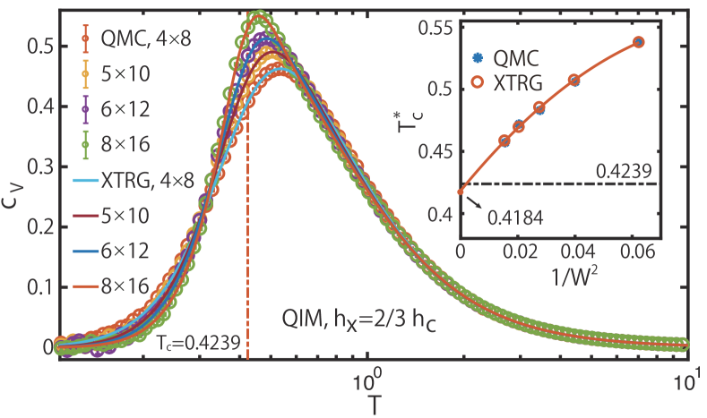
Figure 11: (Color online) Specific heat of QIM for fixed $h_{x}=\frac{2}{3}h_{c}$ on YC $W{\times}L$ of width up to $W=8$ and length $L=2W$ ($W=7$ curve not shown in the main panel for better readability). The XTRG results retaining up to $D=240$ states coincide with the QMC reference data. In the inset, we collect the peak position $T_{c}^{*}$ of $c_{V}$ curves calculated by QMC and XTRG, which also coincide, and extrapolate towards the exact critical temperature in the thermodynamic limit $x\equiv 1/W^{2}\to 0$ by a second order polynomial fit, having $T_{c}^{*}(x)\simeq-14.5\,x^{2}+2.8\,x+T_{c}^{*}(0)$, with an extrapolated value of $T_{c}^{*}(0)\simeq 0.4184$ (a polynomial fit in $1/W$ leads to a similar value).

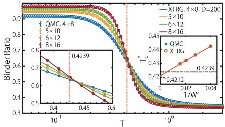
Figure 12: (Color online) Binder ratio curves of QIM for the same $h_{x}=\frac{2}{3}h_{c}$ for YC $W{\times}L$ systems with a fixed aspect ratio $L/W=2$. Left inset zooms in the region near the crossing points $T_{c}^{*}$, and right inset shows a subsequent second-order polynomial extrapolation of $T_{c}^{*}$ to $1/W^{2}\to 0$ (data $W=7$, not shown in the main panel for better readability, is included for the right inset). A second-order polynomial fitting as shown yields an extrapolated $T_{c}^{*}(0)\simeq 0.4212$, which is in excellent agreement with $T_{c}\simeq 0.4239$ in the thermodynamic limit Czarnik and Dziarmaga (2015).

V.2 Binder ratio and phase transition temperature

However, extracting the thermal transition temperature from plain thermal quantities such as peak position int the specific heat in the previous section, gives rise to larger finite-size errors. According to the finite-size scaling (FSS) theory, higher moments, such as Binder cumulants, offer a more accurate means for determining $T_{c}(0)$. One widely adopted Binder cumulant in QMC simulations is

$$U_{4}=\frac{\langle(S_{\mathrm{tot}}^{z})^{2}\rangle^{2}}{\langle(S_{\mathrm{tot}}^{z})^{4}\rangle},$$ (14)

where $S_{\mathrm{tot}}^{z}=\sum_{i}S_{i}^{z}$ is the total spin. The Binder ratio $U_{4}$ has significantly smaller finite-size corrections, namely, $\sim L^{-2}$ Binder (1981a, b). To be specific, according to Ginzburg-Landau theory, the total magnetization of block spins, i.e., $M_{z}=\sum_{i}\langle S_{i}^{z}\rangle_{\beta}$, obeys the Gaussian distribution. In the infinite $T$ limit, it is easy to verify, via Gaussian integration, that $U_{4}=1/3$, while for the $T\rightarrow 0$ limit, it trivially tends to $U_{4}=1$. Right at $T_{c}$, according to the FSS theory, $U_{4}$ flows to a nontrivial fixed value, i.e., it stays as a constant as the system size $N$ increases (given $N$ large). Therefore, $U_{4}$ curves for different system sizes cross at $T_{c}^{*}$, providing a very accurate determination of the critical temperature $T_{c}$.

With MPO techniques, the two expectation values and their ratio $U_{4}$ in Eq. (14) can be obtained very conveniently. The total moment operator $S_{\mathrm{tot}}^{z}$ has a simple MPO representation of bond dimension $D=2$, from which one can construct an exact representation of $(S_{\mathrm{tot}}^{z})^{2}$ (with $D=3$) and $(S_{\mathrm{tot}}^{z})^{4}$ ($D=5$) at ease.

In Fig. 12 we show the calculated Binder ratio by XTRG and QMC, which again show excellent agreement in both the main panel and insets. The left (bottom) inset zooms in the region in the vicinity of the cross point. Taking the crossing temperature $T_{c}^{*}(W)$ of two curves $W$ and $W+1$ as an estimate of the critical temperature, two $T_{c}^{*}$ data sets are extracted from QMC and XTRG, and plotted vs $1/W^{2}$ in the right inset. Again XTRG and QMC data are virtually on top of each other. The estimate from our largest system size results in $T_{c}^{*}(W=7)\simeq 0.4297$. A second-order polynomial extrapolation $1/W^{2}\to 0$ yields $T_{c}^{*}\simeq 0.4212$, which agrees with the thermodynamic limit in Czarnik and Dziarmaga (2015) to within 0.6%.

V.3 Thermal Entanglement

In the QIM case with a thermal phase transition towards a gapped low-temperature phase, the entanglement entropy features a maximum around the transition temperature. Here we also examine the scaling of MPO entanglement $S_{E}$ vs. $T$ for different bonds at which the system is cut when computing $S_{E}$. The resulting “entanglement landscape” is shown in Fig. 13(a) where we observe a clear ridge line along $T\simeq T_{c}$, i.e., the surmised peak in $S_{E}$ at $T_{c}^{S}\simeq T_{c}$. The shape and location of this peak appears stationary in the center of the system (modulo width of the system), yet varies slightly towards to open boundaries [Fig. 13(b)]. This suggests that the peak position $T_{c}^{S}$ in the bulk can be taken as a good estimate of critical temperature $T_{c}$ of the thermal phase transition.

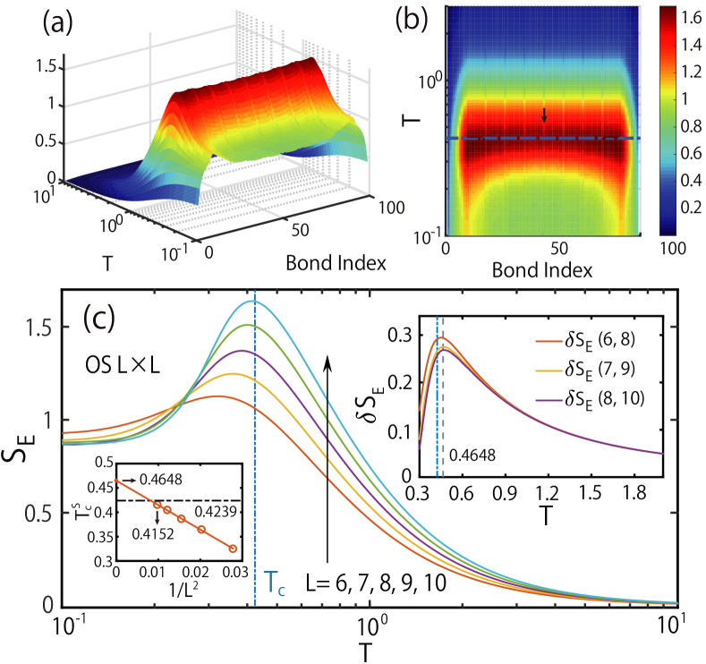
Figure 13: (Color online) (a) Entanglement landscape of QIM thermal states on the OS $10{\times}10$ lattice, for the same $h_{x}=\frac{2}{3}h_{c}$, vs. bond indices and temperature. (b) Top view, showing that the peak temperatures at central bonds (away from boundaries) locate right at the critical temperature $T_{c}$ (horizontal dashed line). (c) $S_{E}$ vs. $T$ on various OS $L{\times}L$ lattices, cut at a central bond [indicated by the the black arrow in (b)] with maximal $S_{E}$. The blue vertical dashed lines in both the main panel and right inset indicate $T_{c}\simeq 0.4239$ in the thermodynamic limit Czarnik and Dziarmaga (2015). The left inset shows the peak temperature $T_{c}^{S}$ vs. inverse system size $1/L^{2}$, which approach the true critical temperature $T_{c}$. $D=240$ bond states are kept in the calculations. The right inset shows the entanglement difference vs. $T$ between consecutive system sizes i.e., OS $L{\times}L$ and OS $L^{\prime}{\times}L^{\prime}$ with $L^{\prime}=L+2$ bearing in mind even-odd effects. The gray vertical dashed line corresponds to the first-order extrapolated value at $1/L^{2}\to 0$ in the left inset.

In Fig. 13(c) therefore we show slices of the entanglement landscape for the bond in the center of the system that maximizes $S_{E}$. Now as we increase $L$ the peak becomes more and more pronounced, and the finite-size estimate of critical temperature $T^{S}_{c}$ approaches the critical temperature $T_{c}$. However, as seen from the inset of Fig. 13(c), while the finite-size $T_{c}^{S}$ appears well-suited for extrapolation in $1/L^{2}\to 0$ in principle, when doing so, the resulting value based on the present data would actually significantly overshoot the true critical temperature, as $T_{c}^{S}\simeq 0.4648$. A similar behavior is also seen on YC geometries (not shown). Hence, so far $S_{E}$ does not lend itself to an simple extrapolation to obtain an accurate critical thermal transition temperature.

In order to gain some insight into the systematic overshooting in the extrapolation of $T_{c}^{S}$, we plot in the right inset of Fig. 13(c) the entanglement difference $\delta S_{E}(L,L^{\prime})=S_{E}(L^{\prime})-S_{E}(L)$ between OS $L^{\prime}{\times}L^{\prime}$ and OS $L{\times}L$ lattices, with $L^{\prime}$ and $L$ both even or odd (to avoid even-odd oscillation). There are a number of features important for analyzing $S_{E}$. The lines in the inset lie on top of each other for $T>1$, meaning $dS/dW\sim\mathrm{const}$ there in agreement with an area law for the entanglement entropy. Moreover, given that the difference $\delta S_{E}$ for the smallest system sizes in our data upper bounds $\delta S_{E}$ for larger systems, $S_{E}/W$ does not diverge at $T_{c}$, but stays finite, which is in stark contrast, e.g., to the specific heat data.

Moreover, from the analysis in the inset the peak position in the $\delta S_{E}$ data appears to remain above $T_{c}$ in the thermodynamic limit, already consistent with the extrapolated $T_{c}^{S}$ for $1/L^{2}\to 0$ in the left inset of Fig. 13(c). Much of this behavior appears related to the strong asymmetry in $S_{E}$ due to a gapped low-temperature phase. Therefore, for the accurate determination of $T_{c}$ from $S_{E}$, it appears one needs to come up with a different procedure other than just extrapolating the temperature for the maximum in $S_{E}$. Nevertheless, it is an interesting observation that from an entanglement point of view, the maximum in $S_{E}$ can systematically occur above $T_{c}$ even in the thermodynamic limit. The precise location may depend on the geometry, i.e., boundary conditions and aspect ratio of the system, and as such deserves further studies.

VI Summary

In this work, we have employed two TTN algorithms, the SETTN and XTRG approaches, to investigate two prototypical quantum spin models, the square-lattice Heisenberg and transverse-field Ising models. We explore four conventional MPO paths, finding that the snake-like path constitutes an overall favorable choice, due to its smaller entanglement and thus less truncation errors on long cylinders and stripes.

Throughout, we found excellent agreement of SETTN and XTRG data with QMC results of both models. Based on these accurate finite-size thermal data of SLH, we are able to extrapolate to the groundstate energy $u_{g}^{*}\simeq-0.6694(4)$ (from YC8 results), as well as the spontaneous magnetization $m_{S}^{*}\simeq 0.30(1)$, all of which are in good agreement with large-scale QMC results. We extract the well-established renormalized classical behaviors, i.e., the exponential divergence at low $T$, of the structure factor $S(q)$ and correlation length $\xi$ vs. $T$, at the ordering momentum $M$.

We have also explored the thermal entanglement $S_{E}$ in the MPO representations of the equilibrium density matrices. $S_{E}$ exhibits a logarithmic scaling in the SLH, which is likely related to gapless excitations in the model. For QIM with a finite-$T$ phase transition, $S_{E}$ shows a pronounced peak at $T_{c}^{S}$, where the thermal phase transition takes place. Besides, $T_{c}^{*}$ from the crosspoint of Binder ratio curves provides very accurate estimate, i.e., down to below 1% errors, of the critical temperature $T_{c}$ in the thermodynamic limit.

Our benchmark calculations reveal that TTN methods, such as XTRG, are highly efficient and accurate in solving quantum many-body problems at finite $T$. Besides the unfrustrated SLH and QIM systems explored in detail here, XTRG can be applied to more challenging frustrated quantum magnets Chen et al. (2018, 2019). There it may play an essential role in bridging the gap between experimental thermal data of currently numerous spin liquid candidate materials and their microscopic spin models.

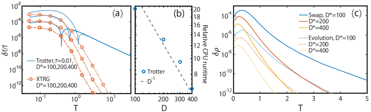
Figure A1: (Color online) (a) Comparison of XTRG and Trotter linear evolution (with swap gates) schemes in the benchmark calculations of an SLH model on OS $4{\times}4$. (b) Computational runtime of the Trotter approach relative to XTRG, which scales roughly as $1/D$ (with the dashed line a guide to the eye). (c) The truncation error analysis in the linear Trotter calculations: the swap gates contribute significantly larger (over two orders of magnitude) truncation errors than those of imaginary-time evolution gates.

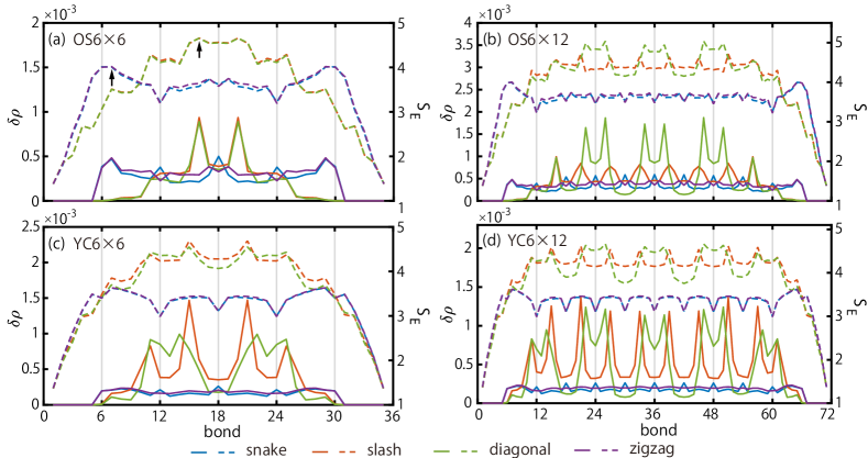
Figure A2: (Color online) Truncation error (solid lines; left axis set) and entanglement entropy $S_{E}$ (dashed lines; right axis set) at a low temperature ($T\simeq 0.06$). The data are obtained by retaining $D^{\ast}=500$ multiplets. We compared the four different mapping paths in Fig. 1, namely, the snake-like, zigzag, diagonal, and slash on (a) OS $6{\times}6$ (b) OS $6{\times}12$ (c) YC $6{\times}6$ and (d) YC $6{\times}12$. The entanglement entropy is precisely also the data that was used for the width of the lines in Fig. 1 in a graphically more organized way.

Appendix A Exponential tensor renormalization group vs. Trotter and swap gates

In thermal tensor network simulations, we start from infinite temperature, $\beta=0$, where $\rho(0)$ has a trivial representation as direct product of identity matrices, to various lower-temperature mixed states. The most straightforward way is to perform such a linear imaginary-time evolution using Trotter gates, which has been widely used Li et al. (2011); Ran et al. (2012); Dong et al. (2017); Czarnik et al. (2012); Czarnik and Dziarmaga (2015); Czarnik et al. (2016, 2017). When applied to 2D systems, given an MPO representation of the density matrix, additional auxiliary swap gates have to be introduced, as adopted in 2D thermal RG methods based on minimally entangled typical thermal states Bruognolo et al. .

On the other hand, a very efficient scheme, XTRG, was proposed in Ref. Chen et al. (2018), where we cooled down the system exponentially following Eq. (4). In Fig. A1, we compare XTRG to the linear evolution with Trotter and swap gates on the SLH model [Eq. (1)] on an OS $4{\times}4$ geometry. In Fig. A1, we choose $\tau=0.01$ in the Trotter decomposition, which constitutes a good compromise in terms of Trotter error relative to truncation error and overall runtime.

As shown in Fig. A1(a), XTRG is found to be more accurate compared to the Trotter scheme, given the same bond dimension. For example, Fig. A1(a) shows that the Trotter data with $D^{*}=400$ ($D\simeq 1600$) yield similar accuracy as XTRG with $D^{*}=200$ ($D\simeq 800$). In addition, the (relative) CPU hours are plotted in Fig. A1(b), showing that the Trotter scheme is slower than XTRG by roughly one order of magnitude. As seen on the log-log scale, however, the relative Trotter performance improves with increasing $D$ roughly as $1/D$, in agreement with the fact that the Trotter approach scales like $O(D^{3})$ and whereas XTRG as $O(D^{4})$. In order to exploit the reduced truncation error with increasing $D$, though, Trotter would also have to reduce the Trotter error by decreasing the Trotter time step, which likely offsets some of the apparent gain with increasing $D$ (note that XTRG is free of Trotter error). Specifically, also note that there is a sign change in $\delta f$ for Trotter, as seen by the downward kink in the $\log|\delta f|$ plot in Fig. A1(a), which moves towards lower temperatures with increasing $D$. Having $\delta f$ change its sign is an indication that the Trotter error is dominant down to lower temperatures, before truncation error sets in.

We explicitly also analyzed truncation and swap gate errors in the 2D Trotter approach in Fig. A1(c). The truncation error due to swap gates (which help bring together two spins with “long-range” interactions after 1D mapping) are about two orders of magnitude greater than those produced directly in the imaginary-time evolution. Therefore, from Fig. A1(c) we observe that the Trotter approach in 2D accumulates significant swap-gate truncation error, and thus it is not competitive in both efficiency and accuracy.

Appendix B Entanglement Entropy and Truncation Errors in Various MPO Paths

Here we provide more detailed information on the entanglement and truncation errors on each MPO bond. In Fig. A2, we show them on four lattices including the OS $6{\times}(6,12)$ and YC $6{\times}(6,12)$, where the same $S_{E}$ data was also used in Fig. 1 to visually demonstrated the entanglement along the various mapping paths. The present discussion therefore extends the analysis of the mapping paths in Sec. III.

Quite generally, in Fig. A2 the truncation error $\delta\rho$ is largest where the block entanglement $S_{E}$ is largest, such that peaks coincide (particularly for the slash and diagonal paths). On the OS $6{\times}6$ and YC $6{\times}6$ lattices, the slash and diagonal paths show peaks in the central part while the zigzag and snake-like lines peak near both ends [indicated by arrows in Fig. A2(a)]. Note, however, the YC $6{\times}6$ case is already seen to be different from that on the OS $6{\times}6$. In Fig. A2(c), the slash and diagonal lines have larger entanglement as well as truncation errors, than those in the zigzag and snake-like paths, not only in the very center but also extended to regions near both ends.

For lattices with larger length $L$, the entanglement and truncation peaks appear periodically in the bulk for all mappings. As illustrated in Figs. A2(b,d), the zigzag and snake-like paths show peaks still near the open boundary and behave rather uniformly in the bulk. This is in contrast to the slash and diagonal paths which have higher $S_{E}$ overall, and thus perform (considerably) worse.

Appendix C Data extrapolation vs. truncation error $\delta\rho$

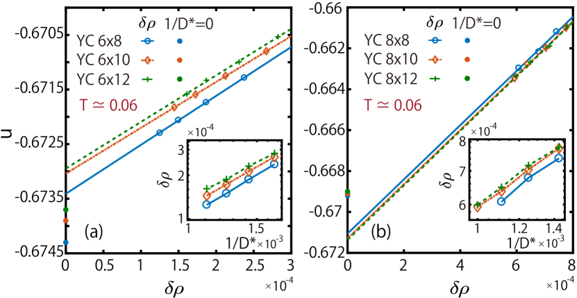
Figure A3: (Color online) The energy per site $u$ vs. truncation error $\delta\rho$ on (a) YC6 and (b) YC8 geometries at $T\simeq 0.06$ [same as in Fig. 5(f) of the main text]. A clear linear $u$ vs. $\delta\rho$ relation is observed and employed to perform the extrapolation. The thus extrapolated $u$ values are in a very good consistency to $1/D^{\ast}{\to}0$ analysis (asterisks), with relative error $\sim$ 0.1%. Insets in (a,b) show $\delta\rho$ vs $1/D^{*}$ on a log-log scale, showing polynomial scaling.

In XTRG simulations, we can only retain a finite number of multiplets $D^{*}$. This introduces a truncation error $\delta\rho$ in the MPO representation of the many-body density matrix. We showed in Figs. 5(c,f) that the low-temperature results for our largest cylinders (say, YC6 or 8) are no longer fully converged, in that for example the internal energy $u$ still varies by about 1% when extrapolating $1/D^{\ast}\to 0$

Nevertheless, to get a flavor on how reliable the extrapolation vs. $1/D^{\ast}\to 0$ is, we do a similar analysis here, but vs. $\delta\rho\to 0$, which represents the truncation error across the geometric bond in the middle of the MPO. In Fig. A3, we show $u$ vs. $\delta\rho$ for the YC6 and YC8 lattice of various lengths, at fixed temperature $T/J\simeq 0.06$.

Having sufficiently large $D^{\ast}$ (sufficiently small $\delta\rho$), similar to the $1/D^{\ast}$ extrapolation in the main paper, we find an approximate linear relationship between $u$ and $\delta\rho$ which can be extrapolated to $\delta\rho\to 0$, equivalent to the infinite $D^{*}$ limit. The results are compared to extrapolated data in $1/$$D^{\ast}$ in Figs. 5(c, f) of the main text, where a good agreement can be seen, for either YC6 and YC8 cases.

The linear relation $\delta u\propto\delta\rho$ can be understood as follows. The truncation error $\delta\rho$ in density matrix $\rho(\frac{\beta}{2})$ directly translates into an error of the partition function $\mathcal{Z}(\beta)=\rm{Tr}\bigl{[}\rho^{\dagger}(\frac{\beta}{2})\,\rho(\frac{\beta}{2})\bigr{]}$, since the latter precisely resembles the cost function itself for optimizing $\rho(\frac{\beta}{2})$. This argument is hand-wavy, of course, since to be specific, we choose for $\delta\rho$ the truncation error after a two-site variational optimization of MPO in the center of the system. This is a good estimate for the accuracy, but does not necessarily represent the precise full error in the calculation of $\mathcal{Z}(\beta)$. Following thermodynamic relations, finally, $\delta\rho$ also reflects linearly in the errors of free energy and energy values, i.e., we can argue that also $\delta f$, and therefore $\delta u\propto\delta\rho$ for small $\delta\rho$.

In practice, for more challenging cases, due to the reason that $\delta\rho$ only serves as an approximate estimate of truncation not fully representing the errors in the variational optimization, we find the analysis of $u$ vs. $1/D^{*}$ numerically more stable and accurate, which is therefore adopted in Fig. 5 of the main text.

References

- Chakravarty et al. (1989) S. Chakravarty, B. I. Halperin, and D. R. Nelson, “Two-dimensional quantum Heisenberg antiferromagnet at low temperatures,” Phys. Rev. B 39, 2344–2371 (1989).
- Greven et al. (1994) M. Greven, R. J. Birgeneau, Y. Endoh, M. A. Kastner, B. Keimer, M. Matsuda, G. Shirane, and T. R. Thurston, “Spin correlations in the 2D Heisenberg antiferromagnet Sr2CuO2Cl2: Neutron scattering, monte carlo simulation, and theory,” Phys. Rev. Lett. 72, 1096 (1994).
- Elstner et al. (1995) N. Elstner, A. Sokol, R. R. P. Singh, M. Greven, and R. J. Birgeneau, “Spin dependence of correlations in two-dimensional square-lattice quantum Heisenberg antiferromagnets,” Phys. Rev. Lett. 75, 938 (1995).
- Dagotto (2005) Elbio Dagotto, “Complexity in strongly correlated electronic systems,” Science 309, 257–262 (2005).
- Rawl et al. (2017) R. Rawl, L. Ge, H. Agrawal, Y. Kamiya, C. R. Dela Cruz, N. P. Butch, X. F. Sun, M. Lee, E. S. Choi, J. Oitmaa, C. D. Batista, M. Mourigal, H. D. Zhou, and J. Ma, “: A spin- triangular-lattice Heisenberg antiferromagnet in the two-dimensional limit,” Phys. Rev. B 95, 060412 (2017).
- White (1992) S. R. White, “Density matrix formulation for quantum renormalization groups,” Phys. Rev. Lett. 69, 2863–2866 (1992).
- (7) F. Verstraete and J. I. Cirac, “Renormalization algorithms for Quantum-Many Body Systems in two and higher dimensions,” arXiv:0407066 (2004) .
- Verstraete et al. (2008) F. Verstraete, V. Murg, and J. I. Cirac, “Matrix product states, projected entangled pair states, and variational renormalization group methods for quantum spin systems,” Adv. Phys. 57, 143–224 (2008).
- Yan et al. (2011) S. Yan, D. A. Huse, and S. R. White, “Spin-liquid ground state of the Kagome Heisenberg antiferromagnet,” Science 332, 1173–1176 (2011).
- Depenbrock et al. (2012) S. Depenbrock, I. P. McCulloch, and U. Schollwöck, “Nature of the spin-liquid ground state of the Heisenberg model on the Kagome lattice,” Phys. Rev. Lett. 109, 067201 (2012).
- White and Chernyshev (2007) S. R. White and A. L. Chernyshev, “Neél order in square and triangular lattice Heisenberg models,” Phys. Rev. Lett. 99, 127004 (2007).
- Zhu and White (2015) Z.-Y. Zhu and S. R. White, “Spin liquid phase of the - Heisenberg model on the triangular lattice,” Phys. Rev. B 92, 041105 (2015).
- Hu et al. (2015) W.-J. Hu, S.-S. Gong, W. Zhu, and D. N. Sheng, “Competing spin-liquid states in the spin-1/2 Heisenberg model on the triangular lattice,” Phys. Rev. B 92, 140403 (2015).
- Zhu et al. (2018) Z.-Y. Zhu, P. A. Maksimov, S. R. White, and A. L. Chernyshev, “Topography of spin liquids on a triangular lattice,” Phys. Rev. Lett. 120, 207203 (2018).
- Bursill et al. (1996) R. J. Bursill, T. Xiang, and G. A. Gehring, “The density matrix renormalization group for a quantum spin chain at non-zero temperature,” J. Phys. Condens. 8, L583 (1996).
- Wang and Xiang (1997) X. Wang and T. Xiang, “Transfer-matrix density-matrix renormalization-group theory for thermodynamics of one-dimensional quantum systems,” Phys. Rev. B 56, 5061–5064 (1997).
- Xiang (1998) T. Xiang, “Thermodynamics of quantum Heisenberg spin chains,” Phys. Rev. B 58, 9142–9149 (1998).
- Feiguin and White (2005) A. E. Feiguin and S. R. White, “Finite-temperature density matrix renormalization using an enlarged Hilbert space,” Phys. Rev. B 72, 220401 (2005).
- White (2009) S. R. White, “Minimally entangled typical quantum states at finite temperature,” Phys. Rev. Lett. 102, 190601 (2009).
- Stoudenmire and White (2010) E. M. Stoudenmire and S. R. White, “Minimally entangled typical thermal state algorithms,” New J. Phys. 12, 055026 (2010).
- Li et al. (2011) W. Li, S.-J. Ran, S.-S. Gong, Y. Zhao, B. Xi, F. Ye, and G. Su, “Linearized tensor renormalization group algorithm for the calculation of thermodynamic properties of quantum lattice models,” Phys. Rev. Lett. 106, 127202 (2011).
- Dong et al. (2017) Y.-L. Dong, L. Chen, Y.-J. Liu, and W. Li, “Bilayer linearized tensor renormalization group approach for thermal tensor networks,” Phys. Rev. B 95, 144428 (2017).
- Ran et al. (2012) S.-J. Ran, W. Li, B. Xi, Z. Zhang, and G. Su, “Optimized decimation of tensor networks with super-orthogonalization for two-dimensional quantum lattice models,” Phys. Rev. B 86, 134429 (2012).
- Czarnik et al. (2012) P. Czarnik, L. Cincio, and J. Dziarmaga, “Projected entangled pair states at finite temperature: Imaginary time evolution with ancillas,” Phys. Rev. B 86, 245101 (2012).
- Czarnik and Dziarmaga (2015) P. Czarnik and J. Dziarmaga, “Variational approach to projected entangled pair states at finite temperature,” Phys. Rev. B 92, 035152 (2015).
- Czarnik et al. (2017) P. Czarnik, J. Dziarmaga, and A. M. Oleś, “Overcoming the sign problem at finite temperature: Quantum tensor network for the orbital model on an infinite square lattice,” Phys. Rev. B 96, 014420 (2017).
- Czarnik et al. (2016) P. Czarnik, M. M. Rams, and J. Dziarmaga, “Variational tensor network renormalization in imaginary time: Benchmark results in the Hubbard model at finite temperature,” Phys. Rev. B 94, 235142 (2016).
- (28) B. Bruognolo, Z. Zhu, S. R. White, and E. Miles Stoudenmire, “Matrix product state techniques for two-dimensional systems at finite temperature,” arXiv:1705.05578 (2017) .
- Chen et al. (2017) B.-B. Chen, Y.-J. Liu, Z. Chen, and W. Li, “Series-expansion thermal tensor network approach for quantum lattice models,” Phys. Rev. B 95, 161104 (2017).
- Chen et al. (2018) B.-B. Chen, L. Chen, Z. Chen, W. Li, and A. Weichselbaum, “Exponential thermal tensor network approach for quantum lattice models,” Phys. Rev. X 8, 031082 (2018).
- Chen et al. (2019) L. Chen, D.-W. Qu, H. Li, B.-B. Chen, S.-S. Gong, J. von Delft, A. Weichselbaum, and W. Li, “Two temperature scales in the triangular lattice Heisenberg antiferromagnet,” Phys. Rev. B 99, 140404 (2019).
- Hubbard (1963) J. Hubbard, “Electron correlations in narrow energy bands,” Proc. R. Soc. Lond. A 276, 238–257 (1963).
- Hubbard (1979a) J. Hubbard, “The magnetism of iron,” Phys. Rev. B 19, 2626–2636 (1979a).
- Hubbard (1979b) J. Hubbard, “Magnetism of iron. II,” Phys. Rev. B 20, 4584–4595 (1979b).
- Hubbard (1981) J. Hubbard, “Magnetism of nickel,” Phys. Rev. B 23, 5974–5977 (1981).
- Anderson (1952) P. W. Anderson, “An approximate quantum theory of the antiferromagnetic ground state,” Phys. Rev. 86, 694–701 (1952).
- Reger and Young (1988) J. D. Reger and A. P. Young, “Monte carlo simulations of the spin-1/2 Heisenberg antiferromagnet on a square lattice,” Phys. Rev. B 37, 5978–5981 (1988).
- Huse and Elser (1988) D. A. Huse and V. Elser, “Simple variational wave functions for two-dimensional Heisenberg spin-1/2 antiferromagnets,” Phys. Rev. Lett. 60, 2531–2534 (1988).
- Liang et al. (1988) S. Liang, B. Doucot, and P. W. Anderson, “Some new variational resonating-valence-bond-type wave functions for the spin-1/2 antiferromagnetic Heisenberg model on a square lattice,” Phys. Rev. Lett. 61, 365–368 (1988).
- Mermin and Wagner (1966) N. D. Mermin and H. Wagner, “Absence of ferromagnetism or antiferromagnetism in one- or two-dimensional isotropic Heisenberg models,” Phys. Rev. Lett. 17, 1133 (1966).
- Manousakis (1991) E. Manousakis, “The spin- Heisenberg antiferromagnet on a square lattice and its application to the cuprous oxides,” Rev. Mod. Phys. 63, 1–62 (1991).
- Blöte and Deng (2002) H. W. J. Blöte and Y.-J. Deng, “Cluster monte carlo simulation of the transverse Ising model,” Phys. Rev. E 66, 066110 (2002).
- Barthel et al. (2009) T. Barthel, U. Schollwöck, and S. R. White, “Spectral functions in one-dimensional quantum systems at finite temperature using the density matrix renormalization group,” Phys. Rev. B 79, 245101 (2009).
- Zwolak and Vidal (2004) M. Zwolak and G. Vidal, “Mixed-state dynamics in one-dimensional quantum lattice systems: A time-dependent superoperator renormalization algorithm,” Phys. Rev. Lett. 93, 207205 (2004).
- Elstner et al. (1993) N. Elstner, R. R. P. Singh, and A. P. Young, “Finite temperature properties of the spin-1/2 Heisenberg antiferromagnet on the triangular lattice,” Phys. Rev. Lett. 71, 1629–1632 (1993).
- Schollwöck (2011) Ulrich Schollwöck, “The density-matrix renormalization group in the age of matrix product states,” Ann. Phys. 326, 96–192 (2011).
- Dubail (2017) J. Dubail, “Entanglement scaling of operators: a conformal field theory approach, with a glimpse of simulability of long-time dynamics in ,” J. Phys. A 50, 234001 (2017).
- Prosen and Pižorn (2007) T. Prosen and I. Pižorn, “Operator space entanglement entropy in a transverse Ising chain,” Phys. Rev. A 76, 032316 (2007).
- (49) T. Barthel, “One-dimensional quantum systems at finite temperatures can be simulated efficiently on classical computers,” arXiv:1708.09349 (2017) .
- Weichselbaum (2012) A. Weichselbaum, “Non-abelian symmetries in tensor networks: A quantum symmetry space approach,” Annals of Physics 327, 2972 – 3047 (2012).
- Xiang et al. (2001) T. Xiang, J.-Z. Lou, and Z.-B. Su, “Two-dimensional algorithm of the density-matrix renormalization group,” Phys. Rev. B 64, 104414 (2001).
- Sandvik (2010) A. W. Sandvik, “Computational studies of quantum spin systems,” AIP Conference Proceedings 1297, 135 (2010).
- Bauer et al. (2011) B. Bauer et al., “The ALPS project release 2.0: open source software for strongly correlated systems,” J. Stat. Mech. 2011, P05001 (2011).
- Okabe and Kikuchi (1988) Y. Okabe and M. Kikuchi, “Monte Carlo study of quantum spin system on the square lattice,” Journal de Physique Colloques 49, C8–1393–C8–1394 (1988).
- Mazurenko et al. (2017) A. Mazurenko, C. S. Chiu, G. Ji, M. F. Parsons, M. Kanász-Nagy, R. Schmidt, F. Grusdt, E. Demler, D. Greif, and M. Greiner, “A cold-atom fermi–Hubbard antiferromagnet,” Nature 545, 462–466 (2017).
- Sandvik (1997) A. W. Sandvik, “Finite-size scaling of the ground-state parameters of the two-dimensional Heisenberg model,” Phys. Rev. B 56, 11678 (1997).
- Chakravarty et al. (1988) S. Chakravarty, B. I. Halperin, and D. R. Nelson, “Low-temperature behavior of two-dimensional quantum antiferromagnets,” Phys. Rev. Lett. 60, 1057 (1988).
- Beard et al. (1998) B. B. Beard, R. J. Birgeneau, M. Greven, and U.-J. Wiese, “Square-lattice Heisenberg antiferromagnet at very large correlation lengths,” Phys. Rev. Lett. 80, 1742 (1998).
- Kim and Troyer (1998) J.-K. Kim and M. Troyer, “Low temperature behavior and crossovers of the square lattice quantum Heisenberg antiferromagnet,” Phys. Rev. Lett. 80, 2705 (1998).
- Elstner et al. (1994) N. Elstner, R. R. P. Singh, and A. P. Young, “Spin-1/2 Heisenberg antiferromagnet on the square and triangular lattices: A comparison of finite temperature properties,” J. Appl. Phys. 75, 5943 (1994).
- Žnidarič et al. (2008) M. Žnidarič, T. Prosen, and I. Pižorn, “Complexity of thermal states in quantum spin chains,” Phys. Rev. A 78, 022103 (2008).
- Orús and Vidal (2009) R. Orús and G. Vidal, “Simulation of two-dimensional quantum systems on an infinite lattice revisited: Corner transfer matrix for tensor contraction,” Phys. Rev. B 80, 094403 (2009).
- Orús (2012) R. Orús, “Exploring corner transfer matrices and corner tensors for the classical simulation of quantum lattice systems,” Phys. Rev. B 85, 205117 (2012).
- Binder (1981a) K. Binder, “Critical properties from Monte Carlo coarse graining and renormalization,” Phys. Rev. Lett. 47, 693–696 (1981a).
- Binder (1981b) K. Binder, “Finite size scaling analysis of Ising model block distribution functions,” Z. Phys. B 43, 119–140 (1981b).