MAANet: Multi-view Aware Attention Networks
for Image Super-Resolution

Abstract.

In most recent years, deep convolutional neural networks (DCNNs) based image super-resolution (SR) has gained increasing attention in multimedia and computer vision communities, focusing on restoring the high-resolution (HR) image from a low-resolution (LR) image. However, one nonnegligible flaw of DCNNs based methods is that most of them are not able to restore high-resolution images containing sufficient high-frequency information from low-resolution images with low-frequency information redundancy. Worse still, as the depth of DCNNs increases, the training easily encounters the problem of vanishing gradients, which makes the training more difficult. These problems hinder the effectiveness of DCNNs in image SR task. To solve these problems, we propose the Multi-view Aware Attention Networks (MAANet) for image SR task. Specifically, we propose the local aware (LA) and global aware (GA) attention to deal with LR features in unequal manners, which can highlight the high-frequency components and discriminate each feature from LR images in the local and the global views, respectively. Furthermore, we propose the local attentive residual-dense (LARD) block, which combines the LA attention with multiple residual and dense connections, to fit a deeper yet easy to train architecture. The experimental results show that our proposed approach can achieve remarkable performance compared with other state-of-the-art methods.

1. Introduction

Image super-resolution (SR) is a hot topic that keeps rising in multimedia and computer vision (Glasner et al., 2009; Dong et al., 2016b; Lim et al., 2017; Haris et al., 2018). It aims at restoring the high-resolution (HR) image from a low-resolution (LR) image via SR algorithms. Image SR is widely used in various applications, including but not limited to medical imaging (Oktay et al., 2018), satellite image analysis (Benecki et al., 2018), security and surveillance (Uiboupin et al., 2016; Yin et al., 2018), high-definition video processing (Huang et al., 2018), etc. Since LR images have lost much information compared to their HR counterparts, the image SR is an ill-posed problem that has multiple solutions for LR inputs (Baker and Kanade, 2002; Lin and Shum, 2004). Recently, with the rapid development of deep learning techniques, deep learning based SR algorithms achieve superior performance over traditional SR algorithms in terms of not only quantitative metrics including peak signal-to-noise ratio (PSNR) and structural similarity index (SSIM), but also qualitative measures with more visually pleasing HR images.

The SR algorithms with deep learning can be grouped into two main-streams. One is based on generative adversarial networks (GANs), involving two neural networks that contest with each other in a zero-sum game framework. This technique helps to generate images that look at least superficially authentic to human observers. Some representative methods include SRGAN (Ledig et al., 2017) and EnhanceNet (Sajjadi et al., 2017). The other is built upon deep convolutional neural networks (DCNNs), which adopts a deep network architecture to learn a mapping from LR images to their HR counterparts with L1 or L2 loss in pixel space. Some representative methods include SRCNN (Dong et al., 2016b), FSRCNN (Dong et al., 2016a), VDSR (Kim et al., 2016), LapSRN (Lai et al., 2017), EDSR (Lim et al., 2017), RDN (Zhang et al., 2018), DBPN (Haris et al., 2018), etc. Generally, the GANs based SR algorithms can obtain more visually pleasing images, contributing to the qualitative performance. However, they do not perform very well in quantitative performance, i.e., PSNR and SSIM. Furthermore, the training of GANs is more difficult and costly for relying on more training data and tough convergence.

In contrast, DCNNs based SR algorithms are much easier to train and can achieve better quantitative performance in PSNR and SSIM. Meanwhile, they are also satisfactory in qualitative performance in real-world applications. In recent years, DCNNs based image SR algorithms have achieved significant improvements and obtained successive state-of-the-art performances over traditional image SR algorithms. However, most of them do not pay enough attention to the limited high-frequency information from LR images. This motivates our idea that to highlight the high-frequency components from LR inputs and to deal with LR features unequally are also of crucial importance for restoring better quality HR images.

To solve these problems, in this paper we propose the local aware (LA) and global aware (GA) attention to adaptively handle LR features in unequal manners. On the one hand, the LA attention unequally highlights the high-frequency components within each LR feature map in the local view. On the other hand, in the global view, the GA attention focuses on unequally re-weighting each feature map after the LR inputs pass through the upscale unit in the HR feature space. Furthermore, to achieve a deeper yet easy training network architecture, we propose the local attentive residual-dense (LARD) block to combine the LA attention with multiple residual and dense connections in the LR feature space. Extensive experiments show a remarkable performance improvement of our model compared with other existing methods.

Our contributions can be summarized as follows. (1) We propose the local aware (LA) attention to highlight the high-frequency components from LR inputs. (2) We propose the global aware (GA) attention to deal with each LR features and re-weight them in unequal manners. (3) We propose the LARD block to construct a very deep and trainable network architecture.

Figure 1. Framework of MAANet

2. Related Work

2.1. Super-Resolution with DCNNs

Recently, traditional super-resolution (SR) algorithms (Li and Orchard, 2001; Zhang and Wu, 2006; Sun et al., 2008; Tai et al., 2010; Yang and Yang, 2013) are severely inferior to multiple DCNNs based SR algorithms. Among them, SRCNN (Dong et al., 2016b) is the pioneering work of DCNNs for image SR task. It first uses bicubic to scale up the LR inputs to HR size and then outperforms traditional image SR algorithms by using only three convolutional layers. Extended from SRCNN, FSRCNN (Dong et al., 2016a) with a deeper network architecture obtains faster speed and better results by scaling up LR inputs to HR size at the last few layers. VDSR (Kim et al., 2016) increases the network depth to a very high level and demonstrates the depth of networks is of crucial importance to image SR task. LapSRN (Lai et al., 2017) is based on a cascade of CNNs, which progressively predicts the sub-band residuals in a coarse-to-fine fashion and obtains progressive reconstruction. EDSR (Lim et al., 2017) removes unnecessary modules in conventional residual networks to enhance the deep super-resolution model and further improves it by expanding the model size while stabilizing the training procedure. RDN (Zhang et al., 2018) proposes to fully exploit the hierarchical features from all the convolutional layers by using residual dense connections to extract abundant local features, and by fusing them to jointly and adaptively learn global hierarchical features in a holistic way. DBPN (Haris et al., 2018) constructs mutually connected up-sampling and down-sampling stages, each of which represents different types of image degradation and high-resolution components. It iteratively exploits up-sampling and down-sampling layers, and provides an error feedback mechanism for projection errors at each stage. However, most of these methods do not pay enough attention to the limited high-frequency information from LR images. From our observation, high-frequency components refer to the pixel intensities that are rapidly changing in space. Compared to the HR images, the LR images have been ruined by losing much high-frequency information, i.e., sharp contrast edges, and leaving redundant low-frequency information, i.e., smooth gradients. If the restored images contain insufficient high-frequency information, they will appear blurring and missing details, resulting in low visual comfort. In our model, we investigate and solve these problems by our proposed MAANet.

2.2. Attention Mechanism

The attention mechanism stems from the study of human vision. In cognitive science, because of the bottleneck of information processing, humans selectively focus on part of the whole information while ignoring others. Similarly, in multimedia and computer vision fields, the attention mechanism is introduced to bias the allocation of available processing resources towards the most informative components of an input. In recent years, a large number of deep learning models have incorporated the attention mechanisms and achieved promising results. Ba et al. (Ba et al., 2015) extends the attention-based RNN model to multiple objects detection task that learns to localize and recognize multiple objects despite being given only class labels. Some employ attention mechanisms in the visual question answering task, such as generating question-guided attention to image feature maps for each question (Chen et al., 2015), the question-guided spatial attention to images for questions of spatial inference (Xu and Saenko, 2016) and querying an image and inferring the answer multiple times to narrow down the attention to images progressively via stacked attention networks (Yang et al., 2016). Wang et al. (Wang et al., 2017) proposes the residual attention network that composed of multiple attention modules, and can be easily scaled up to hundreds of layers with superior performance. Hu et al. (Hu et al., 2018) proposes the squeeze-and-excitation block combined with attention, which can improve the representational power of a network by explicitly modeling the interdependencies between the channels of its convolutional features. Yan et al. (Yan et al., 2019) uses the attention mechanism combined with a proposed semantic-aware meta-learning framework, in which the model explicitly incorporates class sharing across tasks and focuses on only semantically informative parts of input images in each task for few-shot learning. Despite the progress made, however, the attention mechanism has rarely been utilized in some low-level vision tasks such as image super-resolution. In this paper, we propose to apply attention mechanisms to adaptively handle the input low-resolution features in unequal manners with both local and global views.

3. Proposed Method

3.1. Networks Architecture

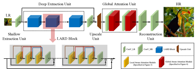
As shown in Figure 1, our MAANet mainly consists of five parts: (1) Shallow extraction unit is exactly a convolution layer (ConV). (2) Deep extraction unit contains several local attentive residual-dense (LARD) blocks in series. It can extract rich deep features with sufficient high-frequency information by combining the LA attention with multiple residual and dense connections. (3) Upscale unit resizes the low-resolution (LR) input to high-resolution (HR) scale. (4) Global attention unit unequally re-weights each feature map in the HR feature space. (5) Reconstruction unit restores the HR output. Considering an input LR image $I_{LR}$, we denote its HR counterpart as $I_{SR}$. In our MAANet, we first input $I_{LR}$ to the shallow feature extraction unit and obtain its shallow feature

(1) $$F_{S}=E_{S}\left(I_{LR}\right),$$

where $E_{S}\left(\cdot\right)$ and $F_{S}$ denote the shallow feature extraction unit and the shallow feature, respectively. Then $F_{S}$ is further inputted to the deep feature extraction unit as

(2) $$F_{D}=E_{D}\left(F_{S}\right),$$

where $F_{D}$ denotes the deep feature and $E_{D}\left(\cdot\right)$ denotes the deep feature extraction unit with $k$ LARD blocks. This unit helps to construct a very deep and trainable network architecture. Next, the obtained deep feature $F_{D}$ continues passing through the upscale unit $E_{U}\left(\cdot\right)$ and resizing to the HR feature maps, i.e.,

(3) $$F_{U}=E_{U}\left(F_{D}\right).$$

The upscaled $F_{U}$ is still on a deep and general stage (Yosinski et al., 2014), so we can further apply the global attention unit to discriminate and re-weight each feature map in the HR feature space. Then we can have

(4) $$F_{G}=E_{G}\left(F_{U}\right),$$

where $E_{G}\left(\cdot\right)$ and $F_{G}$ are the global attention unit and the obtained feature, respectively. Last, the reconstruction unit $E_{R}\left(\cdot\right)$ restores the HR output as

(5) $$I_{SR}=E_{R}\left(F_{G}\right)=\Phi_{MAANet}\left(I_{LR}\right),$$

where $\Phi_{MAANet}\left(\cdot\right)$ denotes the trained networks that map an LR input image $I_{LR}$ to its HR counterpart image $I_{SR}$. The detailed layer and parameter settings for each unit are specified in Section 4.

Similar to most DCNNs based SR algorithms (Dong et al., 2016b, a; Kim et al., 2016; Lai et al., 2017; Lim et al., 2017; Zhang et al., 2018; Haris et al., 2018), we also adopt $L_{1}$ loss to optimize our MAANet. Given a set of training data $\mathcal{D}_{Tr}=\left\{I_{LR}^{i},I_{SR}^{i}\right\}_{i=1}^{n}$, which contains $n$ LR input images and their corresponding HR counterparts. The loss function is defined as:

(6) $$\mathcal{L}\left(\theta\right)=\frac{1}{n}\sum_{i=1}^{n}\left\|\Phi_{MAANet}\left(I_{LR}\right)-I_{SR}\right\|_{1},$$

where $\left\|\cdot\right\|_{1}$ denotes the $L_{1}$ norm and $\theta$ denotes the parameter set of our model.

Figure 2. Local aware attention

3.2. Local Aware Attention

The local aware (LA) attention module is a key building block in our model. Previous DCNNs based SR algorithms normally treat each feature from LR inputs equally in their network layers. However, based on our observation, the LR image has lost much high-frequency information, e.g., sharp contrast edges, textures, etc., compared with its HR counterpart. The LR inputs only contain limited high-frequency components which make the restored HR images visually uncomfortable. Worse still, with low-frequency information redundancy, the SR algorithms are prone to generate overly smooth images to cater to higher quantitative results such as PSNR and SSIM metrics. Therefore, it is of crucial importance to pay more attention to the limited high-frequency information from LR inputs.

Based on these analyses, we propose to deal with each LR feature in unequal manners. First, we deal with LR inputs in the LR feature space. The LA attention module aims to highlight the high-frequency components in the local view, i.e., within each LR feature map in the LR feature space. As shown in Figure 2, we now give more details about the structure of LA attention module. Consider a layer in the deep feature extraction unit, we have a tensor $T_{D}$ with size $H\times W\times C$, which denotes that there are $C$ feature maps in $C$ channels, and each feature map has the height $H$ and the width $W$. We first apply the average pooling to $T_{D}$, i.e.,

(7) $$T_{DA}=AvgPool(T_{D},ks,s),$$

where $ks$ and $s$ are the pooling kernel size and stride, respectively. In this step we set $s=ks$, so that the obtained tensor $T_{DA}$ is with size $\frac{H}{ks}\times\frac{W}{ks}\times C$, and each value in $T_{DA}$ represents the average intensity of a specific sub-region in the corresponding feature map of $T_{D}$. Next, by using up-sampling with a scale parameter equal to $ks$, we can obtain an $H\times W\times C$ tensor $T_{DU}$ that has the same size as $T_{D}$:

(8) $$T_{DU}=UpSampling(T_{DA},ks).$$

The obtained $T_{U}$ can be regarded as an expression of the average smoothness information of the sub-regions in the original $T_{D}$. Essentially, each element in the feature map represents the embedded feature and signal intensity of a specific region in the feature map of the previous layer. So, in order to highlight the high-frequency information in the local view, i.e., the sub-regions of each feature map, we can have an alternative strategy to highlight the elements in each feature map of the next layer. For this purpose, we subtract $T_{DU}$ from $T_{D}$ in element-wise and activate the remainings, i.e.,

(9) $$T_{DR}=Relu\left(T_{D}-T_{DU}\right),$$

where $Relu\left(\cdot\right)$ is the rectified linear unit which takes the positive part of its argument, and $T_{DR}$ is the regional average residual. Each value in $T_{DR}$ denotes whether its corresponding sub-region in the feature map of the previous layer is beyond the average sub-smoothness or not. Last, two shortcuts from $T_{D}$ to $T_{DR}$ (element-wise multiplication), and to the very end (element-wise sum) are constructed as:

(10) $$\hat{T_{D}} =T_{D}+\beta T_{DR}\otimes T_{D},$$

where $\beta$ is a tiny hyper-parameter which controls the degree of highlighting and $\otimes$ denotes the element-wise multiplication. The updated $\hat{T_{D}}$ is then inputted to the next layer of the deep feature extraction unit.

3.3. Global Aware Attention

In contrast to the LA attention, the global aware (GA) attention handles the global view of the LR inputs, i.e., unequally discriminating and re-weighting each feature map after passing through the upscale unit in the HR feature space (Figure 1). Conventional DCNNs based SR algorithms treat each feature map equally in their networks. However, when performing convolution operations, different filters produce different types of features. These features then form different feature maps to represent an input data in multi-level aspects. In other words, the representation ability of each feature map varies from one to another. Therefore, it is necessary to pay more attention to discriminate these feature maps in our model.

Figure 3. Global aware attention

Based on these analyses, we propose the global aware attention unit as shown in Figure 3. We consider an ${H}^{\prime}\times{W}^{\prime}\times C$ tensor $T_{G}$ with the same height ${H}^{\prime}$ and width ${W}^{\prime}$ as HR images. First, we perform a convolution operation with kernel size ${H}^{\prime}\times{W}^{\prime}$ to $T_{G}$, and we can have

(11) $$V_{G}=ConV\left(T_{G},[{H}^{\prime},{W}^{\prime}]\right).$$

The ${H}^{\prime}\times{W}^{\prime}$ filter generates a $1\times 1\times C$ tensor $V_{G}$ for $T_{G}$. Each element in $V_{G}$ denotes some statistics information of each feature map of $T_{G}$. Unlike existing attention models that use global average pooling, we use a trainable ${H}^{\prime}\times{W}^{\prime}$ filter to obtain this statistics information, making the model more robust and expressive. Then by further using two convolution operations to the obtained $V_{G}$, we can have

(12) $${V_{G}}^{\prime}=\sigma\left(ConV_{2}\left(Relu\left(ConV_{1}\left(V_{G},C,{C}^{\prime}\right)\right),{C}^{\prime},C\right)\right),$$

where $ConV_{1}$ is the first convolution operation that shrinks $V_{G}$ from $C$ to ${C}^{\prime}$ channels (${C}^{\prime}<C$), and the second one, i.e., $ConV_{2}$, upscales it back. $Relu\left(\cdot\right)$ and $\sigma\left(\cdot\right)$ are the rectified linear unit and sigmoid gateway, respectively. The updated ${V_{G}}^{\prime}$ can represent a more general global statistics for each feature map in the HR feature space. Last, a shortcut from $T_{G}$ to the updated ${V_{G}}^{\prime}$ is constructed, and the original $T_{G}$ is re-weighted as:

(13) $$\hat{T_{G}}={V_{G}}^{\prime}\cdot T_{G}.$$

With the GA attention, our MAANet can adaptively pay unequal attention to each feature map in the global view.

3.4. LARD Block

Figure 4. LARD block

It has been demonstrated that the depth of networks is of crucial importance to image SR task (Kim et al., 2016). In our MAANet, the deep extraction unit contains several local attentive residual-dense (LARD) blocks in series, as shown in Figure 4. This architecture allows us to easily build a deep yet easy to train networks by repeatedly stacking the LARD block.

As investigated in ResNet (He et al., 2016), as the depth increases, the residual learning framework can dramatically alleviate the problem of vanishing gradients and better guarantee the model’s representation ability by adopting skip connections from one layer to latter layers. The DenseNet (Huang et al., 2017) further extends the skip connections to each single layer and constructs the dense connections in the network architecture. Consequently, one layer receives the feature maps of all preceding layers, resulting in two merits, i.e., deeper trainable network architecture and better cross-layer extraction ability. Inspired by these ideas, the proposed LARD block combines our local aware attention with multiple residual and dense connections, to extract rich deep features from LR inputs. The LARD block can not only highlight the high-frequency components in the local view, i.e., within the sub-regions of each feature map, but also strengthen the model’s extraction and representation ability.

4. Experiments

4.1. Implementation and training details

Our MAANet mainly consists of five parts: shallow extraction unit, deep extraction unit, upscale unit, global attention unit, and reconstruction unit. We now give the implementation details of each part.

First, the shallow extraction unit is exactly a convolution layer which contains 64 filters with the kernel size $3\times 3$ and the stride 1. We ensure the obtained feature maps have the same height and width as the input LR images by adding zero paddings. The obtained feature maps are then inputted to the deep extraction unit, which contains multiple LARD blocks in series. It can extract rich deep features with sufficient high-frequency information. Within each LARD block, there exists three serial microstructures. As shown in Figure 4, each microstructure contains four convolution layers and three LA attention modules. The first three convolution layers are paired with these LA attention modules one by one. Each of these convolution layers contains 32 filters with the kernel size $3\times 3$. The stride is set to 1 and we also use zero paddings to ensure that the obtained feature maps have the same size as LR inputs. The LA attention module has the $4\times 4$ kernel size, and the stride is also set to 4, which makes the sub-region have the same size as the kernel. We construct dense connections among the first three pairs of convolution layer and LA attention module. The fourth convolution layer is added to the end, combined with a residual connection from the beginning to the very end of this microstructure. The residual part is scaled by $\frac{1}{d}$, where $d$ denotes the number of LA attention modules. Last, a wider residual connection from the beginning to the very end of the LARD block is constructed (Figure 1). The residual part is also scaled by a parameter $\frac{1}{k}$, where $k$ denotes the number of microstructures in LARD block. Immediately following the deep extraction unit, the upscale unit is performed to resize the LR feature maps to the size of HR images in height and width. It contains upsample layer with the $nearest$ mode and convolution layer with kernel size $3\times 3$. Next, the global attention unit consisting of two convolution layers and two GL attention modules is added to discriminate and re-weight each feature map in the HR feature space. Each of the convolution layers contains 64 filters with the kernel size $3\times 3$. We set stride as 1 and use zero paddings to ensure the feature maps of the same size as HR images. The parameter $s$ is set to 16 (Figure 3) in the GL attention module, to shrink the number of channels from 64 to 4, and to upscale it back to 64 again to obtain the global statistics for each feature map in the HR feature space. Last, the reconstruction unit with two convolution layers with 64 and 3 filters, respectively, are added in the very end of our model. These two convolution layers also have the kernel size $3\times 3$ and are performed with stride 1 and zero paddings. The reconstruction unit eventually restores the HR outputs.

Figure 5. Sensitivity analysis of $\beta$

As investigated in (Lim et al., 2017; Nah et al., 2017), the batch normalization layers get rid of range flexibility from networks by normalizing the features. So the batch normalization trends to stretch the contrast and normalize the color distribution of images, which destroys the original contrast information. Based on these analyses, we also discard the batch normalization layers in our MAANet to reduce computational complexity, increase the performance and stabilize network training.

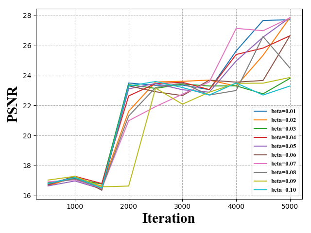
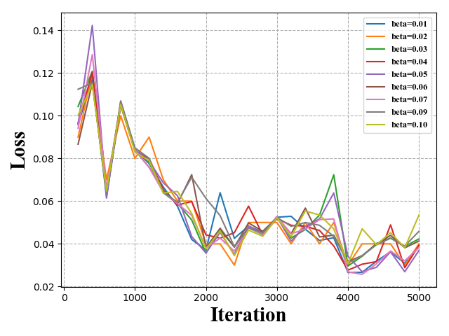
As shown in Eq. (10), there exists a hyper-parameter $\beta$ in our model, which controls the degree of highlighting in the LA attention module. In order to evaluate the sensitivity of $\beta$, we conduct a subset training comparison. We repeatedly train our MAANet on a subset of DIV2K dataset (Timofte et al., 2017), and let $\beta$ range from 0.01 to 0.1, for each individual training. Then we compare the validation results of Set5 (Bevilacqua et al., 2012) for peak signal-to-noise ratio (PSNR) and the training loss of the model. As shown in Figure 5, we can see that as the training goes on, the PSNR gradually increases. Moreover, the greater the iteration of training, the increasing trends of PSNR become more noticeable when $\beta$ is set to 0.07, 0.06, 0.05, and 0.04. As to the training loss, the model has better convergence ability when $\beta$ is set as 0.07, 0.02, and 0.01. Considering both the growth of PSNR and the convergence performance of training loss, we choose to set the $\beta$ at 0.07 in our model.

Our MAANet is implemented by Pytorch and trained with one NVIDIA GTX 1080Ti GPU. We use the stochastic gradient descent to optimize the loss function as shown in Eq. (6). The initial learning rate is set to $2\times 10^{-4}$, and it is evenly halved 5 times throughout the whole training process containing a total of $1\times 10^{6}$ iterations.

4.2. Datasets and Evaluation

Table 1. Description of datasets

Dataset	# of Images	Resolution	Context
Set5 (Bevilacqua et al., 2012)	5	0.2K-0.6K	Natural scenes
Set14 (Zeyde et al., 2010)	14	0.2K-0.8K	Natural scenes
BSDS100 (Zeyde et al., 2010)	100	0.48K	Natural scenes
Urban100 (Huang et al., 2015)	100	$\sim$1K	Urban scenes
Manga109 (Huang et al., 2015)	109	$\sim$1K	Cartoon

Table 2. Quantitative comparison with state-of-the-art competitors

Method	Scale	Set5		Set14		BSDS100		Urban100		Manga109
		PSNR	SSIM	PSNR	SSIM	PSNR	SSIM	PSNR	SSIM	PSNR	SSIM
Bicubic	$\times 2$	33.66	0.9299	30.24	0.8688	29.56	0.8431	26.88	0.8403	30.80	0.9339
SRCNN (Dong et al., 2016b) ($16^{\prime}$)	$\times 2$	36.66	0.9542	32.45	0.9067	31.36	0.8879	29.50	0.8946	35.60	0.9663
FSRCNN (Dong et al., 2016a) ($16^{\prime}$)	$\times 2$	37.05	0.9560	32.66	0.9090	31.53	0.8920	29.88	0.9020	36.67	0.9710
VDSR (Kim et al., 2016) ($16^{\prime}$)	$\times 2$	37.53	0.9590	33.05	0.9130	31.90	0.8960	30.77	0.9140	37.22	0.9750
LapSRN (Lai et al., 2017) ($17^{\prime}$)	$\times 2$	37.52	0.9591	33.08	0.9130	31.08	0.8950	30.41	0.9101	37.27	0.9740
EDSR (Lim et al., 2017) ($17^{\prime}$)	$\times 2$	38.11	0.9602	33.92	0.9195	32.32	0.9013	32.93	0.9351	39.10	0.9773
RDN (Zhang et al., 2018) ($18^{\prime}$)	$\times 2$	38.24	0.9614	34.01	0.9212	32.34	0.9017	32.89	0.9353	39.18	0.9780
DBPN (Haris et al., 2018) ($18^{\prime}$)	$\times 2$	38.09	0.9600	33.85	0.9190	32.27	0.9000	32.55	0.9324	38.89	0.9775
MAANet	$\times 4$	38.37	0.9618	34.33	0.9227	32.42	0.9027	33.47	0.9390	39.63	0.9788
Bicubic	$\times 4$	28.42	0.8104	26.00	0.7027	25.96	0.6675	23.14	0.6577	24.89	0.7866
SRCNN (Dong et al., 2016b) ($16^{\prime}$)	$\times 4$	30.48	0.8628	27.50	0.7513	26.90	0.7101	24.52	0.7221	27.58	0.8555
FSRCNN (Dong et al., 2016a) ($16^{\prime}$)	$\times 4$	30.72	0.8660	27.61	0.7550	26.98	0.7150	24.62	0.7280	27.90	0.8610
VDSR (Kim et al., 2016) ($16^{\prime}$)	$\times 4$	31.35	0.8830	28.02	0.7680	27.29	0.7260	25.18	0.7540	28.83	0.8870
LapSRN (Lai et al., 2017) ($17^{\prime}$)	$\times 4$	31.54	0.8850	28.19	0.7720	27.32	0.7270	25.21	0.7560	29.09	0.8900
EDSR (Lim et al., 2017) ($17^{\prime}$)	$\times 4$	32.46	0.8968	28.80	0.7876	27.71	0.7420	26.64	0.8033	31.02	0.9148
RDN (Zhang et al., 2018) ($18^{\prime}$)	$\times 4$	32.47	0.8990	28.81	0.7871	27.72	0.7419	26.61	0.8028	31.00	0.9151
DBPN (Haris et al., 2018) ($18^{\prime}$)	$\times 4$	32.47	0.8980	28.82	0.7860	27.72	0.7400	26.38	0.7946	30.91	0.9137
MAANet	$\times 4$	32.85	0.9023	29.11	0.7999	27.83	0.7452	26.91	0.8120	31.73	0.9276

Our MAANet is trained on DIV2K dataset (Timofte et al., 2017) with 800 HR images as the training data. The DIV2K contains a broad diversity of contents at 2K resolution that provides many details. To obtain the LR counterparts for training, we downscale the HR images using bicubic and use a batch size of 16 for input LR images. As to the testing phase, we evaluate our model on five widely used benchmark datasets for SR algorithms including Set5 (Bevilacqua et al., 2012), Set14 (Zeyde et al., 2010), BSDS100 (Arbelaez et al., 2011), Urban100 (Huang et al., 2015), and Manga109 (Matsui et al., 2017). These benchmark datasets cover various contents and styles, and include a wide range of resolutions. The description of these testing sets is shown in Table 1.

As to the competitors, we compare our MAANet with 7 state-of-the-art SR algorithms including SRCNN (Dong et al., 2016b), FSRCNN (Dong et al., 2016a), VDSR (Kim et al., 2016), LapSRN (Lai et al., 2017), EDSR (Lim et al., 2017), RDN (Zhang et al., 2018), and DBPN (Haris et al., 2018). The selection criteria for our competitors are: (1) recent work: all of these competitors are published in the most recent years; (2)DCNNs based model: all of these competitors are based on DCNNs and optimized by $L_{1}$ loss function; and (3) competitiveness: they clearly represent the state-of-the-art. All these competitors are trained on the same DIV2K dataset (Timofte et al., 2017) and tested on these five benchmark datasets listed in Table 1. All of them are tuned and compared based on their best performance.

4.3. Quantitative Results

We convert the obtained HR images to YCbCr space, and then compute the peak signal-to-noise ratio (PSNR) and structural similarity index (SSIM) on the Y channel. The PSNR is a commonly used metric to measure the similarity between two images, which is calculated using the Mean-Square-Error (MSE) of the pixels and the maximum possible pixel value. The SSIM is developed to improve traditional methods, such as PSNR, which have been proven to be inconsistent with human visual perception. It takes luminance, contrast, and structure of both images into account. The higher the PSNR and the SSIM, the better the performance of the algorithm. All the competitors and our model are evaluated on the same criteria.

The comparison with state-of-the-art competitors is shown in Table 2. The results are for 2$\times$ and 4$\times$ super-resolution measured by PSNR and SSIM. We can see that our MAANet performs favorably against those competitors on all the evaluated datasets with all scaling factors. Moreover, it is worth noting that with the increase of scaling factors, i.e., from 2$\times$ to 4$\times$, the performance of our MAANet shows a more obvious advantage on these metrics. That is because by using the proposed LA and GA attention, our model can better deal with high-frequency information in the deep feature extraction and the global attention units. In return, it helps to restore more details from the input LR images. The results fully illustrate the superiority of our model.

4.4. Qualitative Results

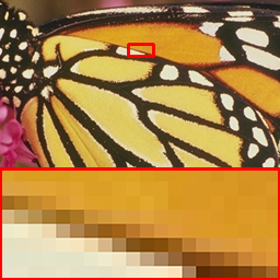
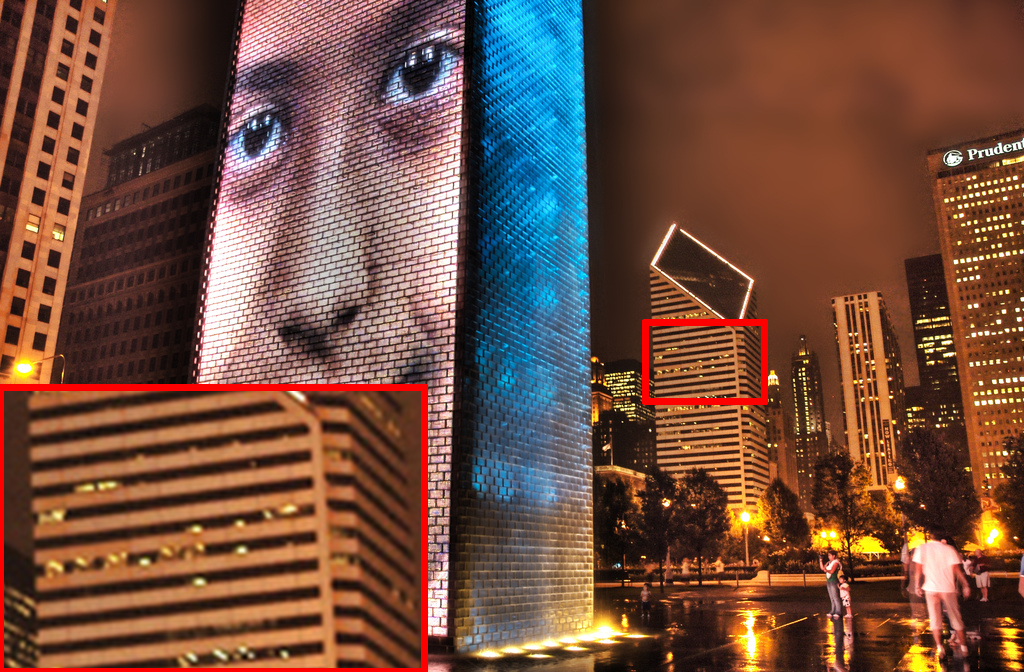
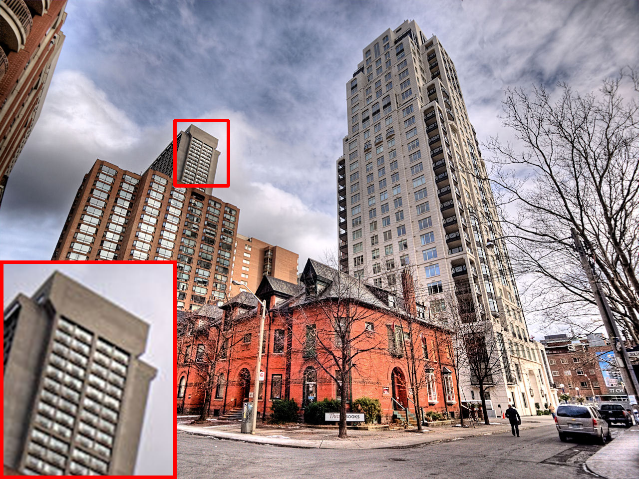
In Figure 7, we show visual comparisons on several images extracted from testing datasets. The results are shown with a scale factor of $4\times$. It can be seen that our MAANet accurately restores the HR images with more details and higher accuracy. For example, the butterfly image is extracted from Set5. Focusing on one tiny square of size $20\times 8$ pixels, we can observe that our model can better recover the actual pixel values with less difference, which endows our model a better performance on PSNR and SSIM. The YumeiroCooking image is extracted from Manga109, which is a challenging dataset containing more stripes and lines. We can see that our model perfectly recovers these stripes and lines in the HR image, and the obtained SR image by our model has much fewer blurred details compared with other competitors. The img_076 and img_020 images are extracted from Urban100, which is also a challenging dataset involving rich contexts of the urban environment. It can be seen that our model recovers more grid patterns and parallel straight lines.

HR (butterflty)

LR

Bicubic

SRCNN (Dong et al., 2016b)

FSRCNN (Dong et al., 2016a)

VDSR (Kim et al., 2016)

LapSRN (Lai et al., 2017)

EDSR (Lim et al., 2017)

RDN (Zhang et al., 2018)

DBPN (Haris et al., 2018)

MAANet

HR (YumeiroCooking)

LR

Bicubic

SRCNN (Dong et al., 2016b)

FSRCNN (Dong et al., 2016a)

VDSR (Kim et al., 2016)

LapSRN (Lai et al., 2017)

EDSR (Lim et al., 2017)

RDN (Zhang et al., 2018)

DBPN (Haris et al., 2018)

MAANet

HR (img_076)

LR

Bicubic

SRCNN (Dong et al., 2016b)

FSRCNN (Dong et al., 2016a)

VDSR (Kim et al., 2016)

LapSRN (Lai et al., 2017)

EDSR (Lim et al., 2017)

RDN (Zhang et al., 2018)

DBPN (Haris et al., 2018)

MAANet

HR (img_020)

LR

Bicubic

SRCNN (Dong et al., 2016b)

FSRCNN (Dong et al., 2016a)

VDSR (Kim et al., 2016)

LapSRN (Lai et al., 2017)

EDSR (Lim et al., 2017)

RDN (Zhang et al., 2018)

DBPN (Haris et al., 2018)

MAANet

Figure 6. Visual comparisons for $4\times$ super-resolution results. LR is the Low-resolution input and HR is the ground-truth high-resolution image.

5. Conclusion

In this paper, we propose a novel image super-resolution model named Multi-view Aware Attention Networks. Our model applies the local aware and the global aware attention to deal with low-resolution images in unequal manners. Our model can highlight the high-frequency components and discriminate each feature from LR images in the local and the global views, respectively. Furthermore, we propose the local attentive residual-dense block that combines the LA attention with multiple residual and dense connections. The LARD block can be easily stacked to fit a very deep and trainable network architecture for the super-resolution task. Extensive evaluations on various benchmark datasets verified the effectiveness of our model against the state-of-the-art SR algorithms.

References

- (1)
- Arbelaez et al. (2011) Pablo Arbelaez, Michael Maire, Charless Fowlkes, and Jitendra Malik. 2011. Contour detection and hierarchical image segmentation. IEEE transactions on pattern analysis and machine intelligence 33, 5 (2011), 898–916.
- Ba et al. (2015) Jimmy Ba, Volodymyr Mnih, and Koray Kavukcuoglu. 2015. Multiple Object Recognition with Visual Attention. In Proceedings of the International Conference on Learning Representations (ICLR).
- Baker and Kanade (2002) Simon Baker and Takeo Kanade. 2002. Limits on super-resolution and how to break them. IEEE Transactions on Pattern Analysis & Machine Intelligence 9 (2002), 1167–1183.
- Benecki et al. (2018) Pawel Benecki, Michal Kawulok, Daniel Kostrzewa, and Lukasz Skonieczny. 2018. Evaluating super-resolution reconstruction of satellite images. Acta Astronautica 153 (2018), 15–25.
- Bevilacqua et al. (2012) Marco Bevilacqua, Aline Roumy, Christine Guillemot, and Marie Line Alberi-Morel. 2012. Low-complexity single-image super-resolution based on nonnegative neighbor embedding. (2012).
- Chen et al. (2015) Kan Chen, Jiang Wang, Liang-Chieh Chen, Haoyuan Gao, Wei Xu, and Ram Nevatia. 2015. Abc-cnn: An attention based convolutional neural network for visual question answering. arXiv preprint arXiv:1511.05960 (2015).
- Dong et al. (2016b) Chao Dong, Chen Change Loy, Kaiming He, and Xiaoou Tang. 2016b. Image super-resolution using deep convolutional networks. IEEE transactions on pattern analysis and machine intelligence 38, 2 (2016), 295–307.
- Dong et al. (2016a) Chao Dong, Chen Change Loy, and Xiaoou Tang. 2016a. Accelerating the super-resolution convolutional neural network. In European conference on computer vision. Springer, 391–407.
- Glasner et al. (2009) Daniel Glasner, Shai Bagon, and Michal Irani. 2009. Super-resolution from a single image. In 2009 IEEE 12th International Conference on Computer Vision (ICCV). IEEE, 349–356.
- Haris et al. (2018) Muhammad Haris, Gregory Shakhnarovich, and Norimichi Ukita. 2018. Deep back-projection networks for super-resolution. In Proceedings of the IEEE conference on computer vision and pattern recognition. 1664–1673.
- He et al. (2016) Kaiming He, Xiangyu Zhang, Shaoqing Ren, and Jian Sun. 2016. Deep residual learning for image recognition. In Proceedings of the IEEE conference on computer vision and pattern recognition. 770–778.
- Hu et al. (2018) Jie Hu, Li Shen, and Gang Sun. 2018. Squeeze-and-excitation networks. In Proceedings of the IEEE conference on computer vision and pattern recognition. 7132–7141.
- Huang et al. (2017) Gao Huang, Zhuang Liu, Laurens Van Der Maaten, and Kilian Q Weinberger. 2017. Densely connected convolutional networks. In Proceedings of the IEEE conference on computer vision and pattern recognition. 4700–4708.
- Huang et al. (2015) Jia-Bin Huang, Abhishek Singh, and Narendra Ahuja. 2015. Single image super-resolution from transformed self-exemplars. In Proceedings of the IEEE Conference on Computer Vision and Pattern Recognition. 5197–5206.
- Huang et al. (2018) Yan Huang, Wei Wang, and Liang Wang. 2018. Video super-resolution via bidirectional recurrent convolutional networks. IEEE transactions on pattern analysis and machine intelligence 40, 4 (2018), 1015–1028.
- Kim et al. (2016) Jiwon Kim, Jung Kwon Lee, and Kyoung Mu Lee. 2016. Accurate image super-resolution using very deep convolutional networks. In Proceedings of the IEEE conference on computer vision and pattern recognition. 1646–1654.
- Lai et al. (2017) Wei-Sheng Lai, Jia-Bin Huang, Narendra Ahuja, and Ming-Hsuan Yang. 2017. Deep laplacian pyramid networks for fast and accurate super-resolution. In Proceedings of the IEEE conference on computer vision and pattern recognition. 624–632.
- Ledig et al. (2017) Christian Ledig, Lucas Theis, Ferenc Huszár, Jose Caballero, Andrew Cunningham, Alejandro Acosta, Andrew Aitken, Alykhan Tejani, Johannes Totz, Zehan Wang, et al. 2017. Photo-realistic single image super-resolution using a generative adversarial network. In Proceedings of the IEEE conference on computer vision and pattern recognition. 4681–4690.
- Li and Orchard (2001) Xin Li and Michael T Orchard. 2001. New edge-directed interpolation. IEEE transactions on image processing 10, 10 (2001), 1521–1527.
- Lim et al. (2017) Bee Lim, Sanghyun Son, Heewon Kim, Seungjun Nah, and Kyoung Mu Lee. 2017. Enhanced deep residual networks for single image super-resolution. In Proceedings of the IEEE Conference on Computer Vision and Pattern Recognition Workshops. 136–144.
- Lin and Shum (2004) Zhouchen Lin and Heung-Yeung Shum. 2004. Fundamental limits of reconstruction-based superresolution algorithms under local translation. IEEE Transactions on Pattern Analysis and Machine Intelligence 26, 1 (2004), 83–97.
- Matsui et al. (2017) Yusuke Matsui, Kota Ito, Yuji Aramaki, Azuma Fujimoto, Toru Ogawa, Toshihiko Yamasaki, and Kiyoharu Aizawa. 2017. Sketch-based manga retrieval using manga109 dataset. Multimedia Tools and Applications 76, 20 (2017), 21811–21838.
- Nah et al. (2017) Seungjun Nah, Tae Hyun Kim, and Kyoung Mu Lee. 2017. Deep multi-scale convolutional neural network for dynamic scene deblurring. In Proceedings of the IEEE Conference on Computer Vision and Pattern Recognition. 3883–3891.
- Oktay et al. (2018) Ozan Oktay, Enzo Ferrante, Konstantinos Kamnitsas, Mattias Heinrich, Wenjia Bai, Jose Caballero, Stuart A Cook, Antonio De Marvao, Timothy Dawes, Declan P O‘Regan, et al. 2018. Anatomically constrained neural networks (ACNNs): application to cardiac image enhancement and segmentation. IEEE transactions on medical imaging 37, 2 (2018), 384–395.
- Sajjadi et al. (2017) Mehdi SM Sajjadi, Bernhard Scholkopf, and Michael Hirsch. 2017. Enhancenet: Single image super-resolution through automated texture synthesis. In Proceedings of the IEEE International Conference on Computer Vision. 4491–4500.
- Sun et al. (2008) Jian Sun, Zongben Xu, and Heung-Yeung Shum. 2008. Image super-resolution using gradient profile prior. In 2008 IEEE Conference on Computer Vision and Pattern Recognition. IEEE, 1–8.
- Tai et al. (2010) Yu-Wing Tai, Shuaicheng Liu, Michael S Brown, and Stephen Lin. 2010. Super resolution using edge prior and single image detail synthesis. In 2010 IEEE Computer Society Conference on Computer Vision and Pattern Recognition. IEEE, 2400–2407.
- Timofte et al. (2017) Radu Timofte, Eirikur Agustsson, Luc Van Gool, Ming-Hsuan Yang, Lei Zhang, Bee Lim, et al. 2017. NTIRE 2017 Challenge on Single Image Super-Resolution: Methods and Results. In The IEEE Conference on Computer Vision and Pattern Recognition (CVPR) Workshops.
- Uiboupin et al. (2016) Tõnis Uiboupin, Pejman Rasti, Gholamreza Anbarjafari, and Hasan Demirel. 2016. Facial image super resolution using sparse representation for improving face recognition in surveillance monitoring. In 2016 24th Signal Processing and Communication Application Conference (SIU). IEEE, 437–440.
- Wang et al. (2017) Fei Wang, Mengqing Jiang, Chen Qian, Shuo Yang, Cheng Li, Honggang Zhang, Xiaogang Wang, and Xiaoou Tang. 2017. Residual attention network for image classification. In Proceedings of the IEEE Conference on Computer Vision and Pattern Recognition. 3156–3164.
- Xu and Saenko (2016) Huijuan Xu and Kate Saenko. 2016. Ask, attend and answer: Exploring question-guided spatial attention for visual question answering. In European Conference on Computer Vision. Springer, 451–466.
- Yan et al. (2019) Shipeng Yan, Songyang Zhang, Xuming He, et al. 2019. A Dual Attention Network with Semantic Embedding for Few-shot Learning. (2019).
- Yang and Yang (2013) Chih-Yuan Yang and Ming-Hsuan Yang. 2013. Fast direct super-resolution by simple functions. In Proceedings of the IEEE international conference on computer vision. 561–568.
- Yang et al. (2016) Zichao Yang, Xiaodong He, Jianfeng Gao, Li Deng, and Alex Smola. 2016. Stacked attention networks for image question answering. In Proceedings of the IEEE conference on computer vision and pattern recognition. 21–29.
- Yin et al. (2018) Minghao Yin, Yongbing Zhang, Xiu Li, and Shiqi Wang. 2018. When Deep Fool Meets Deep Prior: Adversarial Attack on Super-Resolution Network. In 2018 ACM Multimedia Conference on Multimedia Conference. ACM, 1930–1938.
- Yosinski et al. (2014) Jason Yosinski, Jeff Clune, Yoshua Bengio, and Hod Lipson. 2014. How transferable are features in deep neural networks?. In Advances in neural information processing systems. 3320–3328.
- Zeyde et al. (2010) Roman Zeyde, Michael Elad, and Matan Protter. 2010. On single image scale-up using sparse-representations. In International conference on curves and surfaces. Springer, 711–730.
- Zhang and Wu (2006) Lei Zhang and Xiaolin Wu. 2006. An edge-guided image interpolation algorithm via directional filtering and data fusion. IEEE transactions on Image Processing 15, 8 (2006), 2226–2238.
- Zhang et al. (2018) Yulun Zhang, Yapeng Tian, Yu Kong, Bineng Zhong, and Yun Fu. 2018. Residual dense network for image super-resolution. In Proceedings of the IEEE Conference on Computer Vision and Pattern Recognition. 2472–2481.