Comparing particle-particle and particle-hole channels of random-phase approximation

Abstract

We present a comparative study of particle-hole and particle-particle channels of random-phase approximation (RPA) for molecular dissociations of different bonding types. We introduced a direct particle-particle RPA scheme, in analogy to the direct particle-hole RPA formalism, whereby the exchange-type contributions are excluded. This allows us to compare the behavior of the particle-hole and particle-particle RPA channels on the same footing. Our study unravels the critical role of exchange contributions in determining behaviors of the two RPA channels for describing stretched molecules. We also made an attempt to merge particle-hole RPA and particle-particle RPA into a unified scheme, with the double-counting terms removed. However, benchmark calculations indicate that a straightforward combination of the two RPA channels does not lead to a successful computational scheme for describing molecular dissociations.

I Introduction

In the past two decades, the random-phase approximation (RPA), originally formulated by Bohm and Pines Bohm and Pines (1951, 1953) for the homogeneous gas of interacting electrons, has been developed into a versatile approach to compute the non-local electron correlation energy in real molecules and materials Heßelmann and Görling (2011a); Eshuis et al. (2012); Ren et al. (2012a); Paier et al. (2012). Successful applications of RPA have been demonstrated for molecules Furche (2001); Fuchs and Gonze (2002); Toulouse et al. (2009); Zhu et al. (2010); Heßelmann and Görling (2011b); Ren et al. (2011); Eshuis and Furche (2011), solids Harl and Kresse (2008, 2009); Harl et al. (2010); Lebègue et al. (2010); Nguyen and de Gironcoli (2009); Lu et al. (2009); Casadei et al. (2012, 2016), surfaces Ren et al. (2009); Schimka et al. (2010), interfaces Mittendorfer et al. (2011); Olsen et al. (2011), and defects Bruneval (2012); Kaltak et al. (2014a, b). As such, RPA sets a new stage for first-principles electronic-structure calculations for real materials. From the methodology point of view, RPA represents a cornerstone connecting ground-state and time-dependent density-functional theory (DFT)Langreth and Perdew (1975); Gunnarsson and Lundqvist (1976); Dobson (1994), the quantum chemistry coupled cluster method Scuseria et al. (2008), and the Green-function based many-body perturbation theory Dahlen et al. (2005); Ren et al. (2012a). In the context of DFT, via the adiabatic connection fluctuation dissipation theorem, the RPA formalism opens an arena to construct advanced exchange-correlation functional in terms of diagrammatic many-body perturbation theory. Further development beyond RPA, aiming at addressing its remaining shortcomings, has been an active research area. The renormalized second-order perturbation theory Paier et al. (2012); Ren et al. (2013), the approximate exchange kernel (AXK) correction Bates and Furche (2013); Chen et al. (2018), and the power-series expansion scheme Erhard et al. (2016) represent the latest developments based on RPA.

In nuclear physics, the above-mentioned RPA approach is referred to as particle-hole RPA (phRPA), because in its formulation the correlation energy is determined in terms of density fluctuations, originating from particle-hole (ph) pair excitations. In parallel to the phRPA, another type of RPA formulation, referred to as particle-particle RPA (ppRPA), is also discussed Ring and Schuck (1980); Blaizot and Ripka (1986). In this case, the correlation energy is obtained from the pairing matrix fluctuation, arising from the process of creating two particles or two holes. From a diagrammatic point of view, phRPA can be viewed as a summation of ring diagrams to infinite order Gell-Mann and Brueckner (1957), whereas the ppRPA can be interpreted as a summation of the so-called ladder diagrams to infinite order Ring and Schuck (1980); Blaizot and Ripka (1986). In a series of seminal papers, Yang and coworkers van Aggelen et al. (2013); Peng et al. (2013); Yang et al. (2013) developed an adiabatic connection formalism which allows to express the exchange-correlation energy in terms of dynamical pairing matrix fluctuation van Aggelen et al. (2013). Within such a formulation, the ppRPA is the leading-order approximation. The performance of ppRPA for thermochemistry has been benchmarked for small molecules, and its quality for describing molecular dissociations has been analyzed in terms of fractional charge and fractional spin errors Yang et al. (2013); van Aggelen et al. (2014). Furthermore, in parallel to time-dependent DFT (TDDFT), the ppRPA formulation has been extended to excited state calculations Peng et al. (2014). Through these pioneering works, Yang and coworkers brought ppRPA to the attention of DFT/materials science communities. The equivalence of ppRPA to ladder coupled cluster doubles theory have been demonstrated independently by Yang’s Group Peng et al. (2013) and Scuseria’s group Scuseria et al. (2013).

Given the fact that there exists two RPA channels, it is natural to ask if it is possible to combine them. From the viewpoint of many-body perturbation theory, they contain distinct diagrams, except at the second order. In a sense, phRPA and ppRPA can be viewed as different ways to “renormalize” the bare second-order correlation energy. For correlated methods, the correlation energy can often be linked to a self-energy (obtained by taking the functional derivative of the correlation energy with respect to the Green function) Luttinger and Ward (1960). For instance, the phRPA correlation energy is intimately connected to the $GW$ self-energy Hedin (1965); Ren et al. (2012a); the ppRPA, on the other hand, is associated with the particle-particle (pp) T-matrix approximation Baym and Kadanoff (1961); Kanamori (1963); Romaniello et al. (2012); Zhang et al. (2017). Physically speaking, phRPA accounts for the non-local screening effect arising from the long-range Coulomb interaction and shows best performance in the high electron density regime. In contrast, the ppRPA (and T-matrix approximation) describes local scattering of hard-core potentials Bethe and Goldstone (1957), and represents a good approximation in the low electron density regime. In the past, attempts have been made to combine the $GW$ approximation and T-matrix approximation for self-energy calculations Romaniello et al. (2012). It is interesting to check if it is possible to merge their counterparts for ground-state correlation energies – phRPA and ppRPA – into one framework. In this work, we implemented ppRPA in the FHI-aims code package Blum et al. (2009); Ren et al. (2012b). Together with our earlier implementation of the phRPA, we are able to make an attempt to check if a useful computational framework can be found by combining phRPA and ppRPA, and moreover, compare the behavior of phRPA and ppRPA in a systematic way.

When comparing the performance of phRPA and ppRPA for molecules’ properties, it is important to note that phRPA by default refers to the direct phRPA, without including the exchange contributions, whereas ppRPA refers to the full ppRPA, with the exchange contributions included. To compare phRPA and ppRPA on the same footing, we also implemented in this work the full phRPA in FHI-aims. This allows us to examine and compare the performance of phRPA and ppRPA for molecular dissociations in an unbiased way.

The rest of the paper is organized as follows. We briefly recapitulate the basic equations of phRPA and ppRPA in Sec. II. This is followed by a description of the implementation and computational details in Sec. III. The major results and discussions of the behavior of the two channels of RPA, as well as their combinations, are presented in Sec. IV for prototypical molecular dimers. Finally, we conclude this work in Sec. V.

II Theory

Here we briefly review the basic equations of phRPA and ppRPA to facilitate the subsequent comparative analysis of the two schemes. More detailed accounts on their theoretical foundations can be found, e.g., in Refs. [Furche, 2001; Fuchs and Gonze, 2002; Heßelmann and Görling, 2011a; Eshuis et al., 2012; Ren et al., 2012a; van Aggelen et al., 2013]. Note that both the phRPA and the ppRPA can be formulated as an approximation to the exchange-correlation energy within Kohn-Sham (KS) DFT via the adiabatic connection framework. While the phRPA correlation energy can be expressed in terms of an integration over the polarization propagator, the ppRPA can be analogously obtained from the pp propagator, or equivalently the pairing density fluctuation van Aggelen et al. (2013). In particular, the ppRPA correlation energy is given by,

$$E_{c}^{\text{ppRPA}}=\dfrac{1}{2\pi i}\int^{+\textit{i}\infty}_{-\textit{i}\infty}\text{Tr}[ln[\textbf{I}-\textbf{K}^{0}(\omega)\textbf{V}]+\textbf{K}^{0}(\omega)\textbf{V}]d\omega\,,$$ (1)

where $\textbf{K}^{0}(\omega)$ is the non-interacting pp propagator,

$$\begin{split}\textbf{K}^{0}_{pq,rs}(\omega)=&\quad\left(\delta_{pr}\delta_{qs}-\delta_{ps}\delta_{qr}\right)\dfrac{\theta(\epsilon_{p}-\epsilon_{F})\theta(\epsilon_{q}-\epsilon_{F})}{\omega-(\epsilon_{p}+\epsilon_{q}-2\mu)+\textit{i}\eta}\\ &-\left(\delta_{pr}\delta_{qs}-\delta_{ps}\delta_{qr}\right)\dfrac{\theta(\epsilon_{F}-\epsilon_{p})\theta(\epsilon_{F}-\epsilon_{q})}{\omega-(\epsilon_{p}+\epsilon_{q}-2\mu)-\textit{i}\eta}\,.\end{split}$$ (2)

with $\theta(x)$ and $\delta_{pr}$ being respectively the Heaviside step function and Kronecker Delta function. Furthermore, $\epsilon_{F}$ is the Fermi energy, and $\mu$ is the chemical potential set at the middle of the gap between the highest occupied molecular orbital (HOMO) and lowest unoccupied molecular orbital (LUMO). Moreover, V is the antisymmetrized two-electron Coulomb integrals,

$$\textbf{V}_{pq,rs}=\langle pq||rs\rangle=\langle pq|rs\rangle-\langle pq|sr\rangle$$

and

$$\langle pq|rs\rangle=\int\dfrac{\phi^{\ast}_{p}(x_{1})\phi^{\ast}_{q}(x_{2})\phi_{r}(x_{1})\phi_{s}(x_{2})}{|\bf{r}_{1}-\bf{r}_{2}|}dx_{1}dx_{2}$$ (3)

with $x_{1}=(\bf{r}_{1},\sigma_{1})$ being the combined spatial-spin coordinate. Here we follow the usual convention that $p,q,r,s$ refer to general single-particle spin-orbitals, whereas $i,j,k,l$ and $a,b,c,d$ being occupied and unoccupied spin-orbitals respectively.

As thoroughly discussed in the literature Furche (2001); Eshuis et al. (2012); Ren et al. (2012a), the phRPA correlation energy has a similar expression as Eq. (1). The key difference is that the non-interacting pp propagator $\textbf{K}^{0}(\omega)$ is replaced by the non-interacting polarization operator (or linear density response function) ${\chi}^{0}$,

$$\begin{split}{\chi}^{0}_{pq,rs}(\omega)=&\quad\delta_{pr}\delta_{qs}\dfrac{\theta(\epsilon_{p}-\epsilon_{F})\theta(\epsilon_{F}-\epsilon_{q})}{\omega-(\epsilon_{p}-\epsilon_{q})+\textit{i}\eta}\\ &-\delta_{pr}\delta_{qs}\dfrac{\theta(\epsilon_{F}-\epsilon_{p})\theta(\epsilon_{q}-\epsilon_{F})}{\omega-(\epsilon_{p}-\epsilon_{q})-\textit{i}\eta}\,.\end{split}$$ (4)

Furthermore, if the Coulomb matrix V is not antisymmetrized (i.e., $\textbf{V}_{pq,rs}=\langle pq|rs\rangle$), one will obtain the so-called direct phRPA ($d$-phRPA), which is the standard RPA method employed in density functional/materials science community. In contrast, if the antisymmetrized V is employed, one will have the full phRPA ($f$-phRPA), which however received much less attention and was only discussed in the quantum chemistry literature McLachlan and Ball (1964); Oddershede et al. (1975); Ángyán et al. (2011); Seeger and Pople (1977). Different from the phRPA, the ppRPA are only implemented and discussed with the antisymmetrized Coulomb interaction van Aggelen et al. (2013); Peng et al. (2013); Yang et al. (2013); van Aggelen et al. (2014). In analogy to phRPA, in this work we shall term the standard ppRPA with antisymmetrized Coulomb integrals the full ppRPA ($f$-ppRPA), and the one without antisymmetrizing the Coulomb integrals as direct ppRPA ($d$-ppRPA). As mentioned above, this enables us to benchmark phRPA and ppRPA on an equal footing, separating the effect arising from the exchange interactions and that arising from the ph or pp channel itself.

The RPA correlation energy can be calculated using Eq. (1), with the frequency integration being carried out along the imaginary axis. In case of the direct phRPA, the imaginary frequency integration combined with the resolution-of-identity approximation Eshuis et al. (2010); Ren et al. (2012b) leads to an efficient $O(N^{4})$ scaling algorithm, with $N$ being the basis size of the system. An alternative way to obtain the phRPA correlation energy is to cast the RPA equations into the following generalized eigenvalue problem McLachlan and Ball (1964); Furche (2001); Scuseria et al. (2008); Mori-Sanchez et al. (2012),

$$\begin{pmatrix}\textbf{A}&\textbf{B}\\ \textbf{B${}^{\ast}$}&\textbf{A${}^{\ast}$}\end{pmatrix}\begin{pmatrix}X\\ Y\end{pmatrix}=\omega_{n}\begin{pmatrix}\textbf{1}&0\\ 0&-\textbf{1}\end{pmatrix}\begin{pmatrix}X\\ Y\end{pmatrix}$$ (5)

where $A$, $B$, $X$, $Y$ are square matrices of dimension $N_{h}N_{p}\times N_{h}N_{p}$, with $N_{h}$ and $N_{p}$ being the number of occupied (hole) and unoccupied (particle) orbitals respectively. The eigenvalues $\omega_{n}$ form a vector of dimension $N_{h}N_{p}$, and correspond to the neutral excitation energies at the RPA level. In case of full phRPA,

$$A_{ia,jb} =\langle\Phi_{i}^{a}|\hat{H}-E_{0}|\Phi_{j}^{b}\rangle=\delta_{ij}\delta_{ab}(\epsilon_{a}-\epsilon_{i})+\langle aj||ib\rangle$$

$$B_{ia,jb} =\langle\Phi_{0}|\hat{H}-E_{0}|\Phi_{ij}^{ab}\rangle=\langle ij||ab\rangle$$ (6)

where $\hat{H}$ is the Hamiltonian of interacting electrons, $E_{0}=\langle\Phi_{0}|\hat{H}|\Phi_{0}\rangle$ is the Hartree-Fock ground-state energy, with $\Phi_{0}$ being the lowest-energy single Slater determinant. In Eq. (6), $\Phi_{i}^{a}$ and $\Phi_{ij}^{ab}$ are singly and doubly excited configurations, respectively. The corresponding full phRPA (f-phRPA) correlation energy can be obtained as McLachlan and Ball (1964)

$$E^{\textit{f}\textnormal{-phRPA}}_{c}=\frac{1}{4}\left(\sum_{n}\omega_{n}-Tr\{A\}\right)\,.$$ (7)

By contrast, the direct phRPA excitation energies and amplitudes can be obtained by solving Eq. (5) with

$$A_{ia,jb} =\delta_{ij}\delta_{ab}(\epsilon_{a}-\epsilon_{i})+\langle aj|ib\rangle$$

$$B_{ia,jb} =\langle ij|ab\rangle$$ (8)

i.e., without antisymmetrizing the two-electron Coulomb integrals in the construction of $A$ and $B$. Now the $d$-phRPA correlation energy is given by

$$E^{\textit{d}\textnormal{-phRPA}}_{c}=\frac{1}{2}\left(\sum_{n}\omega_{n}-Tr\{A\}\right)\,.$$ (9)

Note that the choice of different prefactors in Eq. (7) and (9) is to ensure that both theories have the correct behavior at second order McLachlan and Ball (1964); Ángyán et al. (2011); Heßelmann (2011). However, the choice of a factor of $1/2$ in Eq. (7) has also been used in the literature Scuseria et al. (2013). The meaning of $d$-phRPA correlation energy can be interpreted as the difference of correlated and uncorrelated electronic zero-point plasmonic energies Furche (2008).

The ppRPA, instead, can be cast into the following matrix equation van Aggelen et al. (2013); Scuseria et al. (2013),

$$\begin{pmatrix}\textbf{C}&\textbf{B}\\ \textbf{B}^{\dagger}&\textbf{D}\end{pmatrix}\begin{pmatrix}X\\ Y\end{pmatrix}=\omega_{n}\begin{pmatrix}\textbf{1}&0\\ 0&-\textbf{1}\end{pmatrix}\begin{pmatrix}X\\ Y\end{pmatrix}$$ (10)

where

$$C_{ab,cd} =\langle\Psi_{0}|\hat{c}_{a}\hat{c}_{b}\left(\hat{H}-E_{0}\right)\hat{c}^{\dagger}_{c}\hat{c}^{\dagger}_{d}|\Phi_{0}\rangle$$

$$=\delta_{ac}\delta_{bd}(\epsilon_{a}+\epsilon_{b}-2\mu)+\langle ab||cd\rangle$$ (11)

$$D_{ij,kl} =\langle\Psi_{0}|\hat{c}^{\dagger}_{i}\hat{c}^{\dagger}_{j}\left(\hat{H}-E_{0}\right)\hat{c}_{k}\hat{c}_{l}|\Phi_{0}\rangle$$

$$=-\delta_{ik}\delta_{jl}(\epsilon_{i}+\epsilon_{j}-2\mu)+\langle ij||kl\rangle\,.$$ (12)

In Eq. (12), $\hat{c}^{\dagger}_{p}(\hat{c}_{p})$ is the creation (annihilation) operator for a single-particle state $p$. Due to the symmetry properties of the above integrals, within losing generality, the orbital indices can be restricted to $i<j,k<l$, and $a<b,c<d$. The indices of matrices $C$ and $D$ correspond to particle pairs and hole pairs respectively. The numbers of particle and hole pairs are

$$N_{pp} =N_{p}(N_{p}-1)/2\,,$$

$$N_{hh} =N_{h}(N_{h}-1)/2\,.$$

Consequently, $C$, $D$ are square matrices of dimensionality $N_{pp}\times N_{pp}$ and $N_{hh}\times N_{hh}$ respectively. On the other hand, in contrast with the phRPA case, $B$ in Eq. (10) becomes a rectangular matrix of $N_{pp}\times N_{hh}$,

$$B_{ab,ij}=\langle ab||ij\rangle\,.$$ (13)

The eigenvalues $\omega_{n}$ obtained from Eq. (10) are split into two groups depending on their sign: the positive eigenvalues are the excitation energies of the $(N+2)$-particle system and the negative eigenvalues correspond to (the negative of) excitation energies of the $(N-2)$-particle system. The corresponding f-ppRPA correlation energy can be obtained as

$$E^{\textit{f}\textnormal{-ppRPA}}_{c}=\sum_{n}^{N_{pp}}\omega_{n}^{N+2}-Tr\{C\}\,,$$ (14)

or equivalently

$$E^{\textit{f}\textnormal{-ppRPA}}_{c}=-\sum_{n}^{N_{hh}}\omega_{n}^{N-2}-Tr\{D\}\,.$$ (15)

It is worthwhile to point out that in ppRPA the inclusion of chemical potential $\mu$ in the definition of matrices $C$ and $D$ is not strictly necessary, and the eigenvectors and the final ppRPA correlation energy are not affected by the $\mu$ value. However, it is convenient to do so since then the obtained eigenvalues $\omega_{n}$ can be naturally grouped into positive modes and negative modes, with clear physical meanings as stated above.

In analogy to the $d$-phRPA, the d-ppRPA is defined by solving Eq. (10) with the following definition of $C$, $D$, $B$ matrices,

$$C_{ab,cd} =\delta_{ac}\delta_{bd}(\epsilon_{a}+\epsilon_{b}-2\mu)+\langle ab|cd\rangle$$

$$D_{ij,kl} =-\delta_{ik}\delta_{jl}(\epsilon_{i}+\epsilon_{j}-2\mu)+\langle ij|kl\rangle$$ (16)

$$\,B_{ab,ij} =\langle ab|ij\rangle$$

without antisymmetrizing the two-electron Coulomb integrals. Here, it is important to note that, in contrast with f-ppRPA, for d-ppRPA the orbital index restrictions ($i<j$, $k<l$ and $a<b$, $c<d$) should not be imposed any longer, due to the loss of antisymmetry. The d-ppRPA correlation energy expression is the same as the f-ppRPA case [Eq. (14) or (15)], but $\omega_{n}$ should be the d-ppRPA eigenvalues and $C$/$D$ matrices should be the non-antisymmetrized integrals as defined in Eq. (II). In Fig. 1 we present the Goldstone diagrams Szabo and Ostlund (1989) of second and third orders for $ppRPA$. These diagrams in general have a ladder structure, but those in the upper row with the two legs (particle or hole lines) closed into themselves are direct diagrams and graphically represent the $d$-ppRPA introduced in this work.

Figure 1: Goldstone diagrams of second [graphs (a) and (d)] and third orders [graphs (b), (c), (e), and (f)] for ppRPA, among which the graphs in the upper row [(a), (b), (c)]

correspond to the $d$-ppRPA.

The leading contribution in both ppRPA and phRPA is their corresponding second-order terms, which are the same for the two RPA channels, as can be easily seen from the corresponding Goldstone diagrams. The second-order correlation energy in full phRPA or full ppRPA is equivalent to the Møller-Plesset second order perturbation theory (MP2) Møller and Plesset (1934), if the Hartree-Fock reference is used. In this work, we term the second-order correlation energy as MP2 for convenience, even if the reference state is not obtained from the Hartree-Fock theory. In the same language of phRPA and ppRPA discussed above, we shall term the original MP2 as full MP2 ($f$-MP2), whose correlation energy is given by

$$\begin{split}E^{\textit{f}\text{-MP2}}_{c}=-\dfrac{1}{2}\sum_{ijab}\dfrac{\langle ij|ab\rangle\langle ab||ij\rangle}{\epsilon_{a}+\epsilon_{b}-\epsilon_{i}-\epsilon_{j}}\,.\end{split}$$ (17)

By contrast, the direct MP2 (d-MP2) correlation energy is obtained as 

$$\begin{split}E^{\textit{d}\text{-MP2}}_{c}=-\dfrac{1}{2}\sum_{ijab}\dfrac{\langle ij|ab\rangle\langle ab|ij\rangle}{\epsilon_{a}+\epsilon_{b}-\epsilon_{i}-\epsilon_{j}}\,.\end{split}$$ (18)

Both phRPA and ppRPA contain a subset of diagrams of the coupled cluster double (CCD) theory Cízek (1966); Bishop and Lührmann (1978); Scuseria et al. (2008, 2013); Peng et al. (2013). While both channels of RPA show some promising performance, they also have some known drawbacks. As discussed above, one of the motivations of the present work is to check if it is possible to combine them to arrive at a better theory, while not going to the full CCD method. A straightforward way to combine phRPA and ppRPA is to add them up, while subtracting the double-counted MP2 term,

$${E}^{\text{comb-RPA}}_{c}={E}^{\text{ppRPA}}_{c}+{E}^{\text{phRPA}}_{c}-E^{\text{MP2}}_{c}\,.$$ (19)

In this combined RPA (denoted as “comb-RPA” in the following) scheme, all three correlation energies appearing on the right-hand side are obtained either in their direct or full flavor, but not mixing up the two flavors. The combination of the $f$-phRPA and $f$-ppRPA, with $f$-MP2 subtracted, is termed as $f$-comb-RPA; analogously, the combination of the $d$-phRPA and $d$-ppRPA, with $d$-MP2 subtracted, is termed as $d$-comb-RPA. We emphasize that both f-comb-RPA and d-comb-RPA are free of double-counting effects at all orders.

We would like to point out that the combination scheme defined in Eq. (19), despite being free of double counting, is not derived rigorously from more fundamental theories. It should rather be viewed as an empirical ansatz whose performance needs to check a posteriori. One may also design alternative double-counting-free schemes, .e.g., by simply averaging phRPA and ppRPA, or by combining the two RPA flavors in a range-separation framework. In a pioneering work by Shepherd, Henderson, and Scuseria Shepherd et al. (2014) short-range ppRPA and long-range phRPA are combined. Initial tests of their scheme for homogeneous electron gas show promising performance. In this connection, it is also interesting to compare Eq. (19) to the quasiparticle RPA (qp-RPA) scheme of Scuseria, Henderson, and Bulik Scuseria et al. (2013) which consists in a simple summation of ppRPA and phRPA, without eliminating the double-counted MP2 term. It should also be noted that, in qp-RPA a prefactor of $1/2$ instead of $1/4$ is used for f-phRPA.

III Computational details

Both the direct and full ppRPA equations are implemented within the all-electron, numerical atomic orbital (NAO) based computer code package FHI-aims Blum et al. (2009); Havu et al. (2009); Ren et al. (2012b). FHI-aims primarily employs NAOs as basis functions to expand molecular orbitals, but, if needed, Gaussian-type orbitals (GTOs) can also be used for comparison purpose. The direct phRPA has already been implemented in FHI-aims Ren et al. (2012b), based on the resolution of identity (RI) technique, together with an integration over the imaginary frequency axis. This allows for a relatively efficient $O(N^{4})$ scaling of direct phRPA calculations. However, such a low-scaling algorithm cannot be applied to the full phRPA. In this work, we implemented Eq. (7) and Eq. (9) straightforwardly, which scales as $O(N^{6})$, to obtain both the full and direct phRPA correlation energies. In the $d$-phRPA case, the obtained results agree with the previous RI-based implementation to a high precision. The full ppRPA was implemented in FHI-aims following the work of Yang et al. Yang et al. (2013). The implementation of direct ppRPA is straightforward by replacing the $C$, $D$, $B$ matrices defined in Eqs. (10) and (13) by those defined in Eq. (II). However, due to the loss of symmetry properties, for $d$-ppRPA the dimension of $C$,$D$, $B$ matrices become $N_{p}^{2}\times N_{p}^{2}$, $N_{h}^{2}\times N_{h}^{2}$, and $N_{p}^{2}\times N_{h}^{2}$ respectively as in f-ppRPA for mixed-spin pair channels Yang et al. (2013). The restricted/unrestricted Hartree-Fock (RHF/UHF), MP2 Møller and Plesset (1934); Szabo and Ostlund (1989), and rPT2 Ren et al. (2013) have already been implemented in FHI-aims. In this work, we also implemented the direct MP2, as defined in Eq. (18), in FHI-aims. Our $f$-MP2 and $d$-MP2 calculations can not only be done on top of the HF reference, but also on top of density functional approximations (DFAs).

In addition to the phRPA and ppRPA results, in this work we will also present results of Hartree-Fock, MP2, rPT2, the coupled cluster theory with singles and doubles substitutions (CCSD) Cízek (1966); Bartlett and Musiał (2007), and Multi-Reference Configuration Interaction Single Double (MRCISD) Werner and Knowles (1988) for comparison. The Hartree-Fock, MP2, rPT2, various flavors of RPA calculations are done with FHI-aims. The CCSD calculations are done with the Gaussian 09 W package Frisch et al. with the exception of H2 molecule based on UHF [Fig. 3], for which we used the recent implementation of Shen et al.Shen et al. (2018) in FHI-aims. Finally, MRCISD calculations are done with the COLUMBUS package Lischka et al. (2017).

We examined the binding energy curves of four homo-nuclear dimers, including the covalently bonded hydrogen dimer (H₂) and nitrogen dimer (N₂), the ionically bonded hydrogen fluoride (HF) dimer, and van der Waals (vdW) bound Argon dimer (Ar₂). For the former three dimers, the Gaussian cc-pVTZ T. H. Dunning (1989) basis sets are used, whereas for Ar₂, the aug-cc-pVTZ basis set was used instead. These basis sets admittedly cannot yield converged binding energy curves, but are sufficient for the present purpose, i.e., comparing the qualitative dissociation behavior of molecular dimers obtained by different methods. In Appendix A, the numerical settings employed in our FHI-aims calculations are presented, together with benchmark results of the $f$-ppRPA total energies for a sequence of atoms, in comparison with published results in Ref. [Peng et al., 2013].

IV Results and discussion

We present in this section the calculated results for four closed-shell dimers (H₂, N₂, HF, and Ar₂) and one open-shell dimer (H${}_{2}^{+}$). The obtained results of all correlated methods depend on the reference state on which they are based. For closed-shell molecules spin-restricted references are often used since they provide a stringent test for static correlation errors. However, for stretched bonds spin-unrestricted references can yield lower energies and better behaved dissociation curves, at the price of broken spatial and spin symmetries. In this section, we mainly use RHF as the reference for closed-shell dimers. For H₂, results of correlated methods based on UHF will also be shown for comparison. For the open-shell molecule H${}_{2}^{+}$, as a natural choice the UHF reference will be used. For RPA methods, instead of Hartree-Fock, the KS reference is often used in practical calculations. The influence of preceding reference states obtained with different functionals will be illustrated in the Appendix B by presenting binding energy curves for H₂ and Ar₂ based on the generalized gradient approximation of Perdew, Burke, and Ernzerhof (PBE) Perdew et al. (1996). Basis set superposition errors are not corrected in the presented results, since in this work we are focused on the relative trends of different methods.

IV.1 H₂ and H${}_{2}^{+}$

The dissociation curves of the H₂ and H${}_{2}^{+}$ are of particular interest for testing DFAs and/or quantum chemistry methods. It appears that none of the current DFAs are able to satisfactorily describe the dissociation behavior of both dimers Cohen et al. (2012). Therefore, H₂ and H${}_{2}^{+}$ dimers are the most important target systems for the recent efforts on designing novel electronic-structure methods Zhang et al. (2016a, b). Our purpose here is to examine the behavior of both the direct and full RPA methods, and especially the combination of ppRPA and phRPA (comb-RPA) as defined in Eq. (19), for these two dimers.

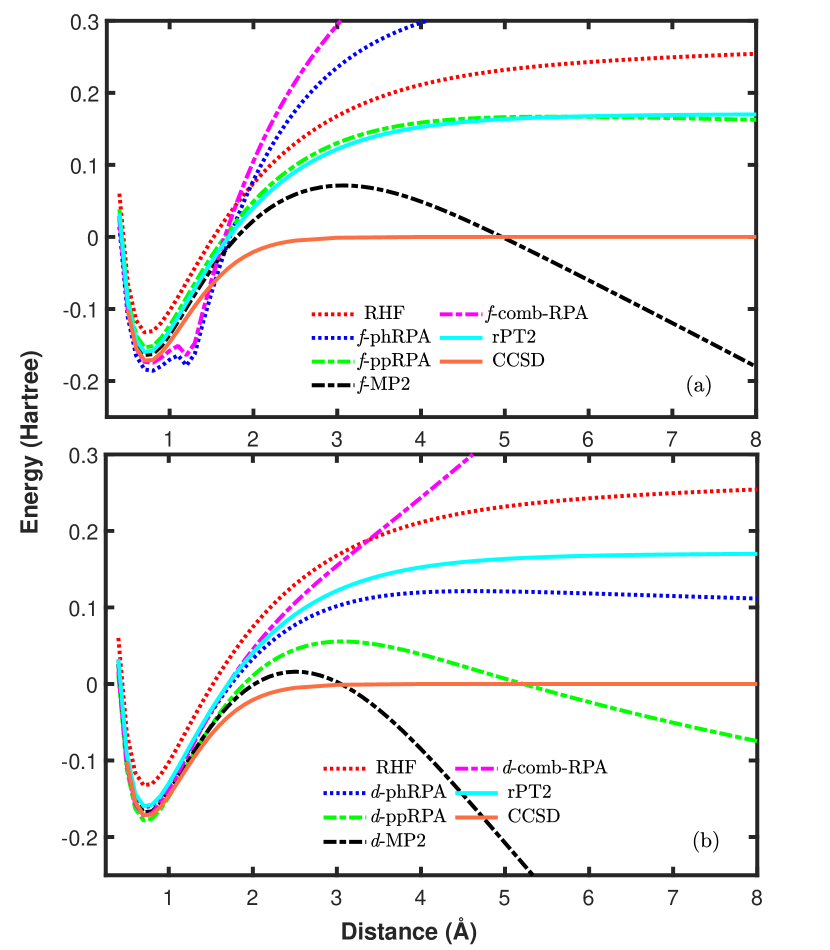
Figure 2: Binding energy curves for $\text{H}_{2}$ with the RHF reference and cc-pVTZ basis set. Panel (a): RPA and MP2 calculations are done with exchange contributions included (full RPA and MP2); panel (b): RPA and MP2 calculations are done without including exchange contributions (direct RPA and MP2). RHF, rPT2, and CCSD results are included in both panels for comparison.

The binding energy curves of H₂ obtained from various methods, based on the RHF reference, are presented in Fig. 2. In panel (a), the results of the full RPA methods, including $f$-ppRPA, $f$-phRPA, and $f$-comb-RPA, are presented, whereas in panel (b), the results from the corresponding direct RPA methods are presented. The $f$-MP2 and $d$-MP2 results are also included in panel (a) and (b) respectively. In addition, the rPT2 and CCSD results are presented in both panels for comparison. Note that the latter two methods are treated here as they are originally, without being further separated into direct and full flavors. Especially the CCSD results are exact for one- and two-electron systems, and hence should be regarded as the reference here. In this case, since the Hartree-Fock reference is used, the rPT2 method reduces to RPA+SOSEXGrüneis et al. (2009); Paier et al. (2010). To highlight the influence of the preceding functionals on the obtained results, in the Appendix B, the same plots, albeit with the PBE reference, are presented (cf. Fig. 8).

All RPA methods describe the H₂ molecule satisfactorily around the equilibrium bond length. For stretched H₂, the f-phRPA becomes unstable around the Coulson-Fisher point Coulson and Fischer (1949) and the binding energy curve has a cusp for the bonding distance around 1.3 Å. Compared to the direct RPA methods, the corresponding full RPA methods are more repulsive, indicating that the exchange contributions give rise to a positive contribution to the binding energies of the H₂ dimer. All RPA methods, except for $d$-ppRPA, are too repulsive for the stretched H₂. Namely, they yield an energy that is too high for the stretched H₂ dimer, similar to the behavior of RHF. Only at the dissociation limit (not shown here), $d$-phRPA and $f$-ppRPA have been shown to yield the correct total energy (i.e., twice of the energy of an isolated H atom) Fuchs and Gonze (2002); Heßelmann and Görling (2011b); van Aggelen et al. (2013), although the asymptotic behavior of these methods is still incorrect. In contrast, MP2 yields an energy that is too low for the stretched dimer, and the MP2 energy becomes diverging in the dissociation limit. At the intermediate bonding distance, the $d$-MP2 is more negative than the $f$-MP2, indicating again that the exchange contribution is positive. The behavior of $d$-ppRPA is somewhat similar to MP2, giving a binding energy that is too low at large bonding distances. Putting phRPA and ppRPA together, the comb-RPA defined in Eq. (19) leads to even more repulsive binding energies for stretched H₂, as can be seen in Fig. 2(a,b) for both the full and direct RPA flavors. Mathematically, by subtracting the very negative MP2 total energy, it comes out naturally that the resultant comb-RPA total energies are much too high. Also, the instability problem of $f$-phRPA around the Coulson-Fisher point is inherited by the $f$-comb-RPA result. In summary, although the comb-RPA scheme as defined in Eq. (19) is free of double-counting, it unfortunately does not work in practice for molecular dissociations, in both full and direct flavors of RPA schemes, if one insists using spin-restricted references. Furthermore, from this comparative study, it is also clear that the phRPA behaves better in its direct flavor, whereas the ppRPA behaves better in its full flavor. The $d$-phRPA and $f$-ppRPA are indeed the usual choice in the literature.

The situation is however quite different if the UHF reference is used. The UHF binding energy curve coincides with the RHF one around the equilibrium distance; beyond the Coulson-Fischer point, the UHF energy is consistently lower, and follows correct asymptotic behavior towards the dissociation limit. On top of UHF, all correlated methods can produce the correct dissociation limit of H₂. However, the $f$-phRPA binding energy curve displays a well-known cusp around the Coulson-Fischer point and this pathological behavior carries over to the corresponding $f$-comb-RPA. Other RPA schemes, as well as MP2 and rPT2, don’t suffer from this problem. However, the binding energy curves from these methods appear to decay faster to zero compared to the reference CCSD@UHF reference. Note that for H₂, the results from CCSD@RHF and CCSD@UHF are identical, and both are exact.

Figure 3: Binding energy curves for H₂ with the UHF reference and cc-pVTZ basis set. Panel (a): full RPA/MP2 results; panel (b): direct RPA/MP2 results. The plots here differ from Fig. 2 only that the UHF reference instead of RHF is used.

Figure 4: Binding energy curves for $\text{H}_{2}^{+}$ with the UHF reference and cc-pVTZ basis set. Panel (a): RPA and MP2 calculations are done with exchange contributions included (full RPA and MP2); panel (b): RPA and MP2 calculations are done without including exchange contributions (direct RPA and MP2). UHF, rPT2, and CCSD results are included in both panels for comparison.

Similar comparative studies for the dissociation of the H${}_{2}^{+}$ molecule are presented in Fig. 4. Now the system contains only one electron, and the UHF method is exact and is taken as the reference here. All other methods are based on the UHF reference state. Besides the UHF, CCSD and rPT2 are also exact for H${}_{2}^{+}$ in theory. Moreover, all the full RPA schemes, as well as MP2, are able to produce the correct dissociation curves for H${}_{2}^{+}$, as can be seen in Fig. 4(a). The incorporation of the exchange contributions cancels the one-electron self-correlation energy, and consequently the full RPA schemes correctly yield zero correlation energy for H${}_{2}^{+}$. In contrast, both the $d$-phRPA and $d$-ppRPA yield too low energy for stretched H${}_{2}^{+}$, indicating the presence of strong charge delocalization errors in these two approaches. In fact, the problem is even more severe for $d$-MP2, which yields even more negative (and eventually diverging) energy than direct RPA’s. As a consequence, the $d$-comb-RPA binding energy curve becomes much too repulsive for heavily stretched H${}_{2}^{+}$.

In this context, we would like to briefly comment on the delocalization error of the RPA methods. As first pointed out by Mori-Sánchez, Cohen, and Yang Mori-Sanchez et al. (2012), the $d$-phRPA suffers from severe delocalization errors, as manifested in the dissociation of H${}_{2}^{+}$. Here we can see this problem arises from the presence of the artificial one-electron self-correlation energy in $d$-phRPA. In fact, for ppRPA, when the exchange contributions are taken out, the $d$-ppRPA also suffers from this error, though to a less extent. We note that, for H₂, such self-correlation errors are still present in direct RPA. However, the negative self-correlation energy becomes advantageous for H₂ since it cancels the positive RHF energy at the dissociation limit. This is in line with the analysis of Henderson and Scuseria Henderson and Scuseria (2010) that the self-interaction errors of direct phRPA mimics the static correlation effect. The high RHF energy for stretched H₂ stems from the on-site Coulomb interaction of two-electrons occupying the same atom – a “double-occupation” (or ionic) configuration that is unavoidable when a single-determinant description of stretched H₂ is employed. Such a high RHF energy arising from the unphysical ionic configurations was compensated by the negative RPA correlation energy of the magnitude at the dissociation limit. However, since this compensation is not complete except at the infinite separation, and the asymptotic behavior of $d$-phRPA@RHF is still incorrect for dissociating H₂. In summary, $d$-phRPA correlation part itself does not really behave differently for the dissociation of H₂ or H${}_{2}^{+}$. It is the different behavior of the preceding Hartree-Fock calculation in these two systems that leads to an overall drastically different performance of the $d$-phRPA scheme for these two systems.

IV.2 N₂

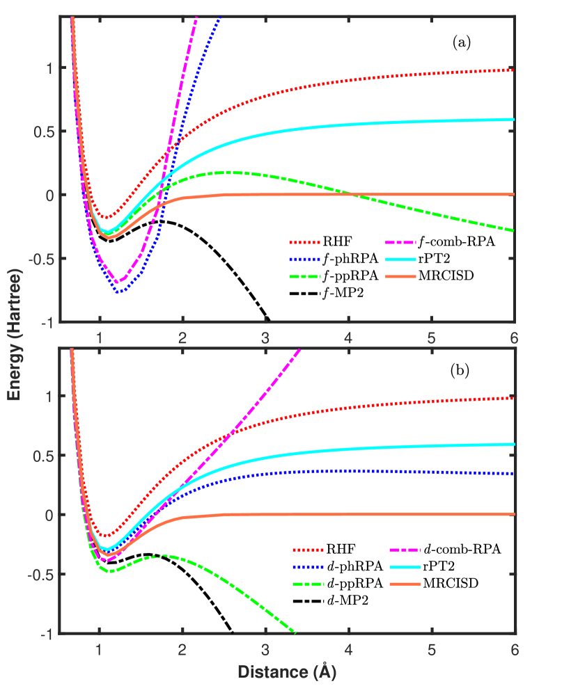
Figure 5: Binding energy curves for $\text{N}_{2}$ with the RHF reference and cc-pVTZ basis set. Panel (a): full RPA/MP2 results; panel (b): direct RPA/MP2 results. The curves are presented in the same way as Fig. 2, except that the reference curve is now given by MRCISD.

Now we look at the triply-bonded nitrogen dimer (N₂). Correctly describing the dissociation behavior of N₂ is a long-standing challenge for any single-reference electronic-structure method. Indeed, for N₂ even the CCSD and CCSD(T) methods do not work, and here we use the results obtained by the multi-reference configuration interaction with single and double excitations (MRCISD) as the reference here. In Fig. 5 we plotted the binding energy curves obtained by full and direct RPA methods (based on the RHF reference) respectively in panel (a) and (b). The full and direct MP2, as well as the rPT2 results are also plotted for comparison. For N₂, the different methods already yield quite different binding energies around the equilibrium distance. The $d$-phRPA was known to be able to produce the correct dissociation limit for N₂ Furche (2001), although a positive bump was formed at intermediate bond lengths. Comparing the results of $f$-phRPA to $d$-phRPA, we see that the exchange terms increase the bond strength (more attractive) around the equilibrium distance while weakening it (more repulsive) at the intermediate and large bonding distances. This results in a very steep binding energy curve with large curvature. Such an (unphysical) feature also carries over to the $f$-comb-RPA scheme, as can be seen from Fig. 5. The $f$-ppRPA performs well around the equilibrium region, but forms a positive bump at the intermediate bonding distances, and eventually goes below the energy zero at large bond lengths.

Comparing panel (a) to panel (b) reveals that the exchange terms, in general, makes the binding energy curve more repulsive at intermediate and large bonding distances, not only for phRPA, but also for ppRPA and MP2. Without including exchange contributions, the binding energies of $d$-ppRPA behaves similar to MP2, and falls below the energy zero already at intermediate bonding distances. The rPT2 (i.e., $d$-phRPA+SOSEX here) result for N₂ behaves similarly to $d$-phRPA and $f$-ppRPA at the equilibrium distance, but saturates at too high energies in the dissociation limit. Similar to the H₂ case, the comb-RPA schemes again performs very badly for N₂. The rising of the $f$-comb-RPA binding energy curve is even steeper than $d$-comb-RPA for increasing bond lengths, arising from a similar behavior of $f$-phRPA.

IV.3 HF

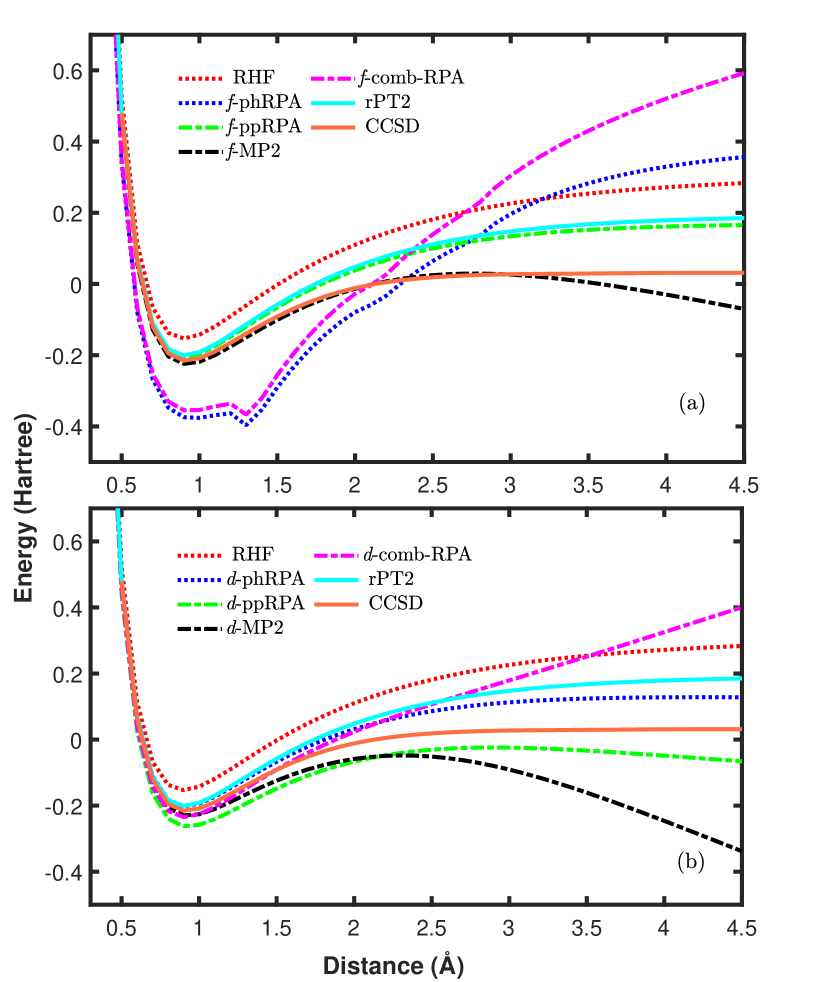
Figure 6: Binding energy curves for hydrogen fluoride (HF) with the RHF reference and cc-pVTZ basis set. Panel (a): full RPA/MP2 results; panel (b): direct RPA/MP2 results. The curves are presented in the same way as Fig. 2.

Next, we examine a dimer of ionic character – the hydrogen fluoride (HF). In Fig. 6, the RHF, RPA, MP2, and rPT2 results for the HF dimer are presented. Now the CCSD result is not exact for the HF dimer, but still provides a high-quality reference. Similar to the N₂ case, the $f$-phRPA already overbinds the HF dimer around the equilibrium distance, suffers from instabilities at bonding distances around 1.4 Å, and gets too repulsive for large bond lengths. Such these behaviors carry over to $f$-comb-RPA. Surprisingly, MP2 performs pretty well at the equilibrium and intermediate bonding distances, but then drops down (and eventually diverging) at large distances. The $f$-ppRPA also performs well around the equilibrium distance, and follows closely the (too repulsive) rPT2 curve for large bond lengths. Removing the exchange contributions, the $d$-phRPA behaves much more reasonably over a wide range of bonding distances. On the other hand, the $d$-ppRPA curve becomes attractive at large bonding distances , and falls below the CCSD curve. The $d$-comb-RPA curve behaves similarly to the $d$-phRPA around the equilibrium distance, but gets too repulsive for large distances, arising from the opposite behavior of $d$-MP2.

IV.4 Ar₂

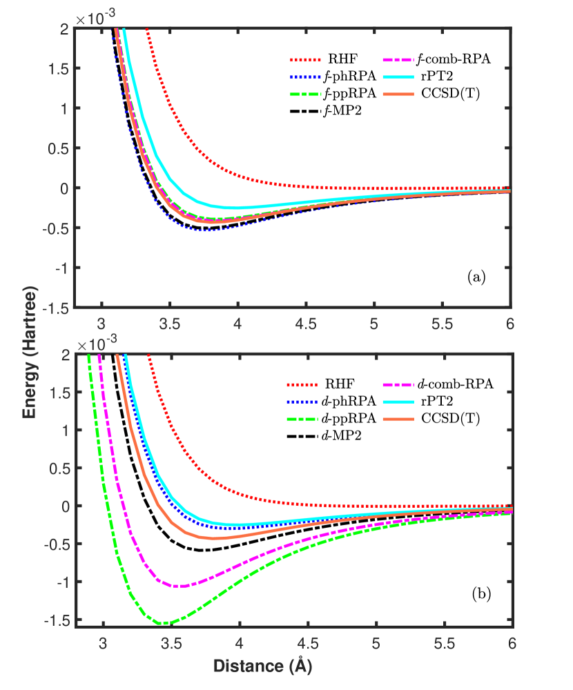
Figure 7: Binding energy curves for Ar₂ with the RHF reference and gaussian aug-cc-pVTZ basis set. Panel (a): full RPA/MP2 results; panel (b): direct RPA/MP2 results. The curves are labeled in the same way as Fig. 2, except that the reference curve is now given by CCSD(T). The frozen-core approximation is used in all correlated calculations.

Finally, we look at a prototypical dimer bound purely by dispersion interactions – Ar₂. The results from various methods are presented in Fig. 7 (a) and (b). One can see that the $f$-ppRPA performs rather well for Ar₂, yielding a binding energy curve that follows closely the CCSD(T) reference curve. In contrast with the covalently and ionically bonded dimers, the $f$-phRPA does not exhibit any pathological behavior for Ar₂. This is because the Ar atom itself has a closed-shell electronic structure, and the RHF solution is stable for Ar₂ for all inter-atomic distances. As a consequence, MP2 is well-behaved for Ar₂, although a well-known overbinding behavior can be noticed. In this case, the $f$-phRPA result closely resembles that of (full) MP2, and putting all three ingredients together, the $f$-comb-RPA performs remarkably well, producing a binding energy curve that is highly accurate.

Remarkably, in the case of Ar₂, the exchange contributions seem to have an opposite effect on phRPA and ppRPA. Without including the exchange contributions, the $d$-phRPA curve become more repulsive, showing a well-known underbinding behavior for Ar₂. On the contrary, the $d$-ppRPA curve becomes much more attractive, vastly overbinding Ar₂. As a consequence, in contrast to $f$-comb-RPA, the $d$-comb-RPA overbinds the Ar₂ dimer significantly. We note that, the rPT2 underbinds Ar₂ in Fig. 7; this is because rPT2 here is based on the RHF reference, and the renormalized singles contribution is not included. The rPT2@PBE scheme instead yields an accurate binding energy curve for Ar₂, as can be seen from Fig 9 in the Appendix B.

V Conclusion

In this work, we implemented the ppRPA scheme within the all-electron, NAO-based code package – FHI-aims. Benchmark calculations show that our implementation, based on the resolution of identity approximation to the two-electron Coulomb integrals, agrees remarkably well with the previous implementation of Peng and coauthors Peng et al. (2013). We performed a systematic comparative study of the behavior of the ppRPA and phRPA for describing the dissociation of diatomic molecules of different bonding characters. The novel aspect in our research is that we introduced a direct ppRPA, whereby the exchange contributions are excluded from the formalism, in a similar fashion as done in the direct phRPA. This allows us to compare phRPA and ppRPA on an equal footing, separately for direct and full RPA flavors. While benchmark calculations show that both phRPA and ppRPA are not able to dissociate correctly all types of dimers, but generally speaking, the phRPA is better employed in its direct flavor, without including the exchange terms (i.e., $d$-phRPA), while the full RPA is better employed in its full flavor, with exchange terms included (i.e., $f$-ppRPA). In this work, we also pointed out the seemingly different performance of $d$-phRPA for H₂ and H${}_{2}^{+}$ mainly arises from the preceding RHF/UHF for H₂ and H${}_{2}^{+}$, and not from the $d$-phRPA correlation energy itself.

In an attempt to combine both phRPA and ppRPA, we examined a simple procedure (Eq. 19), whereby the phRPA and ppRPA correlation energies are added together, with the double-counted second-order (MP2) correlation energy removed. This scheme, although containing no double-counting terms, yields worse and often unphysical results for the dissociation of covalent and ionic diatomic molecules. The behavior stems from the bad performance of MP2 for describing stretched molecules, but is manifested in an opposite way, resulting in too repulsive binding energy curves for large bonding distances. In the quasi-particle RPA scheme examined by Scuseria et al. Scuseria et al. (2013), the phRPA and ppRPA correlation energies are summed up, but the doubly-counted MP2 terms are not excluded. This quasiparticle RPA scheme does not suffer from some of the drastic failures of the comb-RPA scheme examined in this work, but vastly overestimates the total and binding energies of molecular systems. Scuseria et al. Scuseria et al. (2013) attributed this failure to the neglecting of the inter-channel coupling terms between phRPA and ppRPA.

The pertinent question is if it is possible to develop a theory between RPA and CCSD, which is close to RPA in the computational cost, but close to CCSD in the accuracy? The present work shows that it is highly nontrivial to achieve this goal. A straightforward combination of the ph and pp channels of RPA does not work. More investigations along these lines are required to answer this question.

Appendix A Numerical accuracy of our ppRPA implementation in FHI-aims

As mentioned above, in this work we are concentrating on the qualitative features of different computational schemes, rather than presenting highly converged results with respect to the basis set size. To facilitate a direct comparison with literature results, we employed Gaussian basis sets, which are however treated numerically in FHI-aims Blum et al. (2009). The real-space integration are done by a summation over atom-centered overlapping numerical grid. The accuracy of the numerical integration is controlled by two parameters of the spherical grids positioned around each atom: the number of radial integration shells $N_{r}$ and the angular grid points in the outermost radial shell (denoted below as outer_grid). Furthermore, the two-electron Coulomb repulsion integrals (ERI) are evaluated using the resolution-of-identity (RI) approximation. In FHI-aims, the auxiliary basis functions (ABFs) used in the RI expansion are generated from “on-site” products of atomic orbitals, and the redundancy of such products are further eliminated through the Gram-Schmidt orthonormalization procedure Ren et al. (2012b); Ihrig et al. (2015). The accuracy of RI is affected by the number of ABFs, which is in turn controlled by the threshold $\eta$ (keyword prodbas_acc in FHI-aims) in the Gram-Schmidt procedure, and by the threshold $\theta$ (keyword prodbas_threshold) set for singular value decomposition (SVD) of the Coulomb matrix ( in order to invert it) within the ABFs. Thus the numerical accuracy of RPA total energies in FHI-aims, for a given set of single-particle atomic orbitals, are affected both by the numerical integration grid and by the RI accuracy.

In Table 1 we present $f$-ppRPA total energies (more precisely the deviation from the reference value) for the N₂ molecule for a set of successively denser integration grid. From Table 1, one can see that, for $rm>=4$, the error incurred by numerical integration is below 1 meV for the $f$-ppRPA total energy of N₂. Similar accuracy can be achieved for other types of RPA calculations. Table 2 demonstrates the influence of two key parameters involved in the RI approximation on the $f$-ppRPA total energy. One can see that the results here is not much sensitive to the $\eta$ parameter for $\eta>=10^{-2}$, but an appreciable dependence on the $\theta$ parameter is observed. From $\eta<=10^{-4}$, an accuracy better than 1 meV in the RPA total energy for N₂ can be achieved.

Table 1: Deviations (in meV) of f-ppRPA@RHF total energy for N₂ from the reference value due to the real-space integration grid governed by the number of radial shells $N_{r}$ and the angular grid points of the outermost shell $outer\_grid$. In FHI-aims Blum et al. (2009), $N_{r}=rm*N_{r}^{0}$, where $rm=1,2,4,6,\cdots$ is the so-called radial multiplier and $N_{r}^{0}=46$ for the N element. The total energy $E=-2972.67642407$ eV, obtained with $rm=6$ $(N_{r}=276)$ and $outer\_grid=1202$, is taken as the reference value here. The cc-pVTZ basis set is used in the calculation. The parameters $\eta=10^{-2}$ and $\theta=10^{-5}$ are used for used for the RI decomposition of ERIs.

	434	590	770	974	1202
$2(92)$	2.559	2.588	2.554	2.559	2.562
$4(184)$	0.653	0.669	0.652	0.653	0.654
$6(276)$	-0.002	0.014	-0.002	-0.001	0.000

Table 2: Deviations (in meV) of the $f$-ppRPA@RHF total energy from the reference value due to the RI approximation. Here $\eta$ (prodbas_acc) and $\theta$ (prodbas_threshold) are respectively the thresholding parameter for the Gram-Schmidt orthonormalization and for the SVD decomposition. The total energy $E=-2972.67648033$ eV, obtained with $\eta=10^{-4}$ and $\theta=10^{-6}$ is taken as the reference here. In all calculations $rm=6$ and outer_grid=770 are used for the real-space grid integration.

	$10^{-3}$	$10^{-4}$	$10^{-5}$	$10^{-6}$
$10^{-2}$	8.821	0.416	0.058	0.052
$10^{-3}$	7.234	0.212	0.152	0.004
$10^{-4}$	6.636	0.295	0.046	0.000

Finally, to validate our ppRPA implementation in FHI-aims, in Table 3 we present our calculated all-electron $f$-ppRPA total energies, on top of the UHF reference, for a selected set of atoms. Our results obtained using FHI-aims are compared to those of Peng et al.Peng et al. (2013). The ground-state UHF total energies are also presented for comparison. For these calculations, we set $rm=6$ and $outer\_grid=770$ for the grid integration, and $\eta=10^{-4}$ and $\theta=10^{-5}$ for the RI approximation. We see that the differences in both UHF and $f$-ppRPA total energies between our implementation and that of Peng et al.Peng et al. (2013) are vanishingly small – only noticeable at the micro-Hartree ($\mu$Ha) level. Such $\mu$Ha-level error in $f$-ppRPA total energies indicates that our RI-based ppRPA implementation is highly accurate.

Table 3: UHF and $f$-ppRPA@UHF total energies (in Hartree) for a series of atoms. Results obtained in this work are compared to the literature values of Peng et al. Peng et al. (2013). The Cartesian Gaussian cc-pVTZ basis set is used in both works. The “Difference” columns present the UHF/$f$-ppRPA total energy differences between this work and Ref. [Peng et al., 2013].

Atom	HF				$f$-ppRPA
	Ref. Peng et al. (2013)	This work	Difference		Ref. Peng et al. (2013)	This work	Difference
He	-2.861154	-2.861153	0.000001		-2.885608	-2.885608	0.000000
Li	-7.432706	-7.432705	0.000001		-7.443903	-7.443903	0.000000
Be	-14.572875	-14.572875	0.000000		-14.598923	-14.598926	-0.000003
B	-24.532104	-24.532104	0.000000		-24.566435	-24.566439	-0.000004
C	-37.691663	-37.691664	-0.000001		-37.746778	-37.746781	-0.000003
N	-54.400883	-54.400885	-0.000002		-54.482916	-54.482918	-0.000002
O	-74.811910	-74.811913	-0.000003		-74.933839	-74.933844	-0.000005
F	-99.405657	-99.405660	-0.000003		-99.576884	-99.576891	-0.000007
Ne	-128.532010	-128.532015	-0.000005		-128.760771	-128.760771	0.000000

Appendix B Binding energy curves of H₂ and $\text{Ar}_{2}$ based on the PBE reference

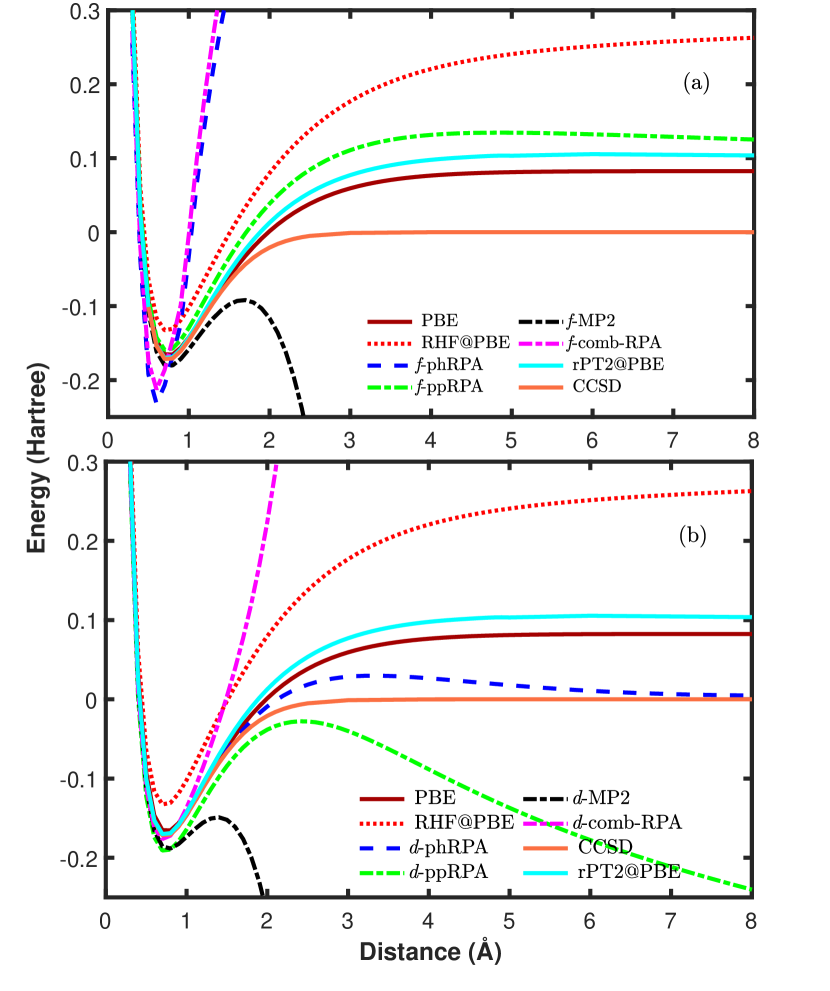
Figure 8: Binding energy curves for $\text{H}_{2}$ with the PBE reference and cc-pVTZ basis set. The plots here differ from Fig. 2 only that, except for CCSD, all other methods are based on the PBE reference instead of RHF.

In Fig 8, we present the binding energy curves for H₂ obtained with RPA, MP2, and rPT2 methods based on the PBE reference.

The CCSD result for H₂ is still the reference curve here. Comparing Fig. 8 to Fig. 2, one can observe that the RPA methods on top of PBE in general yield less repulsive binding energy curves compared to their counterparts on top of RHF. The $f$-phRPA seems to be the exception in the sense that $f$-phRPA@PBE curve is even more repulsive than $f$-phRPA@RHF. This unusual behavior also carries over to $f$-comb-RPA.

In Fig 9, The binding energy curves for Ar₂ obtained with RPA, MP2, and rPT2 methods based on the PBE reference are presented. Now the CCSD(T) curve is the reference curve to compare with. Compared to Fig. 7, one can see that the RPA and MP2 curves show a pronounced dependence on the reference state, shifting downwards when moving from the the RHF reference to the PBE reference. In contrast with $f$-ppRPA@RHF which agrees with the CCSD(T) result pretty well, now $f$-ppRPA@PBE overbinds the Ar₂ dimer substantially. It is even more so for $d$-ppRPA@PBE, with exchange contributions excluded. It is striking that the phRPA shows an opposite trend compared to the ppRPA, in that the $d$-phRPA@PBE is more repulsive than $f$-phRPA@PBE. The comb-RPA curve now sits in between the ppRPA and phRPA curves, for both direct and full flavors. The rPT2@PBE can accurately reproduce the CCSD(T) curve, as already shown in Ref. [Ren et al., 2013].

From the RHF reference to the PBE reference, one can see that the RPA results have undergone substantial changes. A pertinent question is that if an “optimal” reference state can be found for practical RPA calculations. Recently, self-consistent phRPA schemes, in which an “optimal” noninteracting reference is defined and iteratively optimized, are developed by Ye et al. in the generalized optimized effective potential framework Jin et al. (2017) and by Voora et al. Voora et al. (2019) in the generalized KS framework. It has been shown Jin et al. (2017); Voora et al. (2019) that the singles excitation effect Ren et al. (2011) can be automatically included in these schemes.

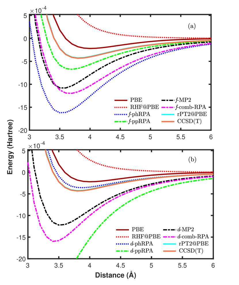
Figure 9: Binding energy curves for Ar₂ with the PBE reference and aug-cc-pVTZ basis set. The plots here differ from Fig. 7 only that, except for CCSD(T), all other methods are based on the PBE reference instead of RHF. The frozen-core approximation is used for the correlated methods.

References

- Bohm and Pines (1951) D. Bohm and D. Pines, Phys. Rev. 82, 625 (1951).
- Bohm and Pines (1953) D. Bohm and D. Pines, Phys. Rev. 92, 609 (1953).
- Heßelmann and Görling (2011a) A. Heßelmann and A. Görling, Mol. Phys. 109, 2473 (2011a).
- Eshuis et al. (2012) H. Eshuis, J. E. Bates, and F. Furche, Theor. Chem. Acc. 131, 1084 (2012).
- Ren et al. (2012a) X. Ren, P. Rinke, C. Joas, and M. Scheffler, J. Mater. Sci. 47, 7447 (2012a).
- Paier et al. (2012) J. Paier, X. Ren, P. Rinke, G. E. Scuseria, A. Grüneis, G. Kresse, and M. Scheffler, New J. Phys. 14, 043002 (2012).
- Furche (2001) F. Furche, Phys. Rev. B 64, 195120 (2001).
- Fuchs and Gonze (2002) M. Fuchs and X. Gonze, Phys. Rev. B 65, 235109 (2002).
- Toulouse et al. (2009) J. Toulouse, I. C. Gerber, G. Jansen, A. Savin, and J. G. Ángyán, Phys. Rev. Lett. 102, 096404 (2009).
- Zhu et al. (2010) W. Zhu, J. Toulouse, A. Savin, and J. G. Ángyán, J. Chem. Phys. 132, 244108 (2010).
- Heßelmann and Görling (2011b) A. Heßelmann and A. Görling, Phys. Rev. Lett. 106, 093001 (2011b).
- Ren et al. (2011) X. Ren, A. Tkatchenko, P. Rinke, and M. Scheffler, Phys. Rev. Lett. 106, 153003 (2011).
- Eshuis and Furche (2011) H. Eshuis and F. Furche, J. Phys. Chem. Lett. 2, 983 (2011).
- Harl and Kresse (2008) J. Harl and G. Kresse, Phys. Rev. B 77, 045136 (2008).
- Harl and Kresse (2009) J. Harl and G. Kresse, Phys. Rev. Lett. 103, 056401 (2009).
- Harl et al. (2010) J. Harl, L. Schimka, and G. Kresse, Phys. Rev. B 81, 115126 (2010).
- Lebègue et al. (2010) S. Lebègue, J. Harl, T. Gould, J. G. Ángyán, G. Kresse, and J. F. Dobson, Phys. Rev. Lett. 105, 196401 (2010).
- Nguyen and de Gironcoli (2009) H.-V. Nguyen and S. de Gironcoli, Phys. Rev. B 79, 205114 (2009).
- Lu et al. (2009) D. Lu, Y. Li, D. Rocca, and G. Galli, Phys. Rev. Lett. 102, 206411 (2009).
- Casadei et al. (2012) M. Casadei, X. Ren, P. Rinke, A. Rubio, and M. Scheffler, Phys. Rev. Lett. 109, 146402 (2012).
- Casadei et al. (2016) M. Casadei, X. Ren, P. Rinke, A. Rubio, and M. Scheffler, Phys. Rev. B 93, 075153 (2016).
- Ren et al. (2009) X. Ren, P. Rinke, and M. Scheffler, Phys. Rev. B 80, 045402 (2009).
- Schimka et al. (2010) L. Schimka, J. Harl, A. Stroppa, A. Grüneis, M. Marsman, F. Mittendorfer, and G. Kresse, Nature Materials 9, 741 (2010).
- Mittendorfer et al. (2011) F. Mittendorfer, A. Garhofer, J. Redinger, J. Klimeš, J. Harl, and G. Kresse, Phys Rev. B 84, 201401(R) (2011).
- Olsen et al. (2011) T. Olsen, J. Yan, J. J. Mortensen, and K. S. Thygesen, Phys. Rev. Lett. 107, 156401 (2011).
- Bruneval (2012) F. Bruneval, Phys. Rev. Lett. 108, 256403 (2012).
- Kaltak et al. (2014a) M. Kaltak, J. Klimeš, and G. Kresse, J. Chem. Theory Comput. 10, 2498 (2014a).
- Kaltak et al. (2014b) M. Kaltak, J. Klimeš, and G. Kresse, Phys. Rev. B 90, 054115 (2014b).
- Langreth and Perdew (1975) D. C. Langreth and J. P. Perdew, Solid State Commun. 17, 1425 (1975).
- Gunnarsson and Lundqvist (1976) O. Gunnarsson and B. I. Lundqvist, Phys. Rev. B 13, 4274 (1976).
- Dobson (1994) J. F. Dobson, in Topics in Condensed Matter Physics, edited by M. P. Das (Nova, New York, 1994).
- Scuseria et al. (2008) G. E. Scuseria, T. M. Henderson, and D. C. Sorensen, J. Chem. Phys. 129, 231101 (2008).
- Dahlen et al. (2005) N. E. Dahlen, R. van Leeuwen, and U. von Barth, Int. J. Quantum Chem. 101, 512 (2005).
- Ren et al. (2013) X. Ren, P. Rinke, G. E. Scuseria, and M. Scheffler, Phys. Rev. B 88, 035120 (2013).
- Bates and Furche (2013) J. E. Bates and F. Furche, J. Chem. Phys. 139, 171103 (2013).
- Chen et al. (2018) G. P. Chen, M. M. Agee, and F. Furche, J. Chem. Theo. Comput. 14, 5701 (2018).
- Erhard et al. (2016) J. Erhard, P. Bleiziffer, and A. Görling, Phys. Rev. Lett. 117, 143002 (2016).
- Ring and Schuck (1980) P. Ring and P. Schuck, The Nuclear Many-Body Problem (Springer, 1980).
- Blaizot and Ripka (1986) J. P. Blaizot and G. Ripka, Quantum Theory of Finite Systems (MIT Press, 1986).
- Gell-Mann and Brueckner (1957) M. Gell-Mann and K. A. Brueckner, Phys. Rev. 106, 364 (1957).
- van Aggelen et al. (2013) H. van Aggelen, Y. Yang, and W. Yang, Phys. Rev. A 88, 030501(R) (2013).
- Peng et al. (2013) D. Peng, S. N. Steinmann, H. van Aggelen, and W. Yang, J. Chem. Phys. 139, 104112 (2013).
- Yang et al. (2013) Y. Yang, H. van Aggelen, S. N. Steinmann, D. Peng, and W. Yang, J. Chem. Phys. 139, 174110 (2013).
- van Aggelen et al. (2014) H. van Aggelen, Y. Yang, and W. Yang, J. Chem. Phys. 140, 18A511 (2014).
- Peng et al. (2014) D. Peng, H. van Aggelen, Y. Yang, and W. Yang, J. Chem. Phys. 140, 18A522 (2014).
- Scuseria et al. (2013) E. Scuseria, T. M. Henderson, and I. W. Bulik, J. Chem. Phys. 139, 104113 (2013).
- Luttinger and Ward (1960) J. M. Luttinger and J. C. Ward, Phys. Rev. 118, 1417 (1960).
- Hedin (1965) L. Hedin, Phys. Rev. 139, A796 (1965).
- Baym and Kadanoff (1961) G. Baym and L. P. Kadanoff, Phys. Rev. 124, 287 (1961).
- Kanamori (1963) J. Kanamori, Prog. Theor. Phys. 30, 275 (1963).
- Romaniello et al. (2012) P. Romaniello, F. Bechstedt, and L. Reining, Phys. Rev. B 85, 155131 (2012).
- Zhang et al. (2017) D. Zhang, N. Q. Su, and W. Yang, J. Phys. Chem. Lett. 8, 3223 (2017).
- Bethe and Goldstone (1957) H. A. Bethe and J. Goldstone, Proc. R. Soc. London A 238, 551 (1957).
- Blum et al. (2009) V. Blum, F. Hanke, R. Gehrke, P. Havu, V. Havu, X. Ren, K. Reuter, and M. Scheffler, Comp. Phys. Comm. 180, 2175 (2009).
- Ren et al. (2012b) X. Ren, P. Rinke, V. Blum, J. Wieferink, A. Tkatchenko, A. Sanfilippo, K. Reuter, and M. Scheffler, New J. Phys. 14, 053020 (2012b).
- McLachlan and Ball (1964) A. D. McLachlan and M. A. Ball, Rev. Mol. Phys. 36, 844 (1964).
- Oddershede et al. (1975) J. Oddershede, P. Jörgensen, and N. H. F. Beebe, J. Chem. Phys. 63, 2996 (1975).
- Ángyán et al. (2011) J. G. Ángyán, R.-F. Liu, J. Toulouse, and G. Jansen, J. Chem. Theory Comput. 7, 3116 (2011).
- Seeger and Pople (1977) R. Seeger and J. A. Pople, J.Chem. Phys. 66, 3045 (1977).
- Eshuis et al. (2010) H. Eshuis, J. Yarkony, and F. Furche, J. Chem. Phys. 132, 234114 (2010).
- Mori-Sanchez et al. (2012) P. Mori-Sanchez, A. J. Cohen, and W. Yang, Phys. Rev. A 85, 042507 (2012).
- Heßelmann (2011) A. Heßelmann, J. Chem. Phys. 134, 204107 (2011).
- Furche (2008) F. Furche, J. Chem. Phys. 129, 114105 (2008).
- Szabo and Ostlund (1989) A. Szabo and N. S. Ostlund, Modern Quantum Chemistry: Introduction to Advanced Electronic Structure Theory (McGraw-Hill, New York, 1989).
- Møller and Plesset (1934) C. Møller and M. S. Plesset, Phys. Rev. 46, 618 (1934).
- Cízek (1966) J. Cízek, J. Chem. Phys. 45, 4256 (1966).
- Bishop and Lührmann (1978) R. F. Bishop and K. H. Lührmann, Phys. Rev. B 17, 3757 (1978).
- Shepherd et al. (2014) J. J. Shepherd, T. M. Henderson, and G. E. Scuseria, Phys. Rev. Lett. 112, 133002 (2014).
- Havu et al. (2009) V. Havu, V. Blum, P. Havu, and M. Scheffler, J. Comp. Phys. 228, 8367 (2009).
- Bartlett and Musiał (2007) R. J. Bartlett and M. Musiał, Rev. Mod. Phys. 79, 291 (2007).
- Werner and Knowles (1988) H. J. Werner and P. J. Knowles, J. Chem. Phys. 89, 5803 (1988).
- (72) M. J. Frisch, G. W. Trucks, H. B. Schlegel, G. E. Scuseria, M. A. Robb, J. R. Cheeseman, G. Scalmani, V. Barone, B. Mennucci, G. A. Petersson, et al., Gaussian∼09W Revision D.01, gaussian Inc. Wallingford CT 2009.
- Shen et al. (2018) T. Shen, I. Y. Zhang, and M. Scheffler, arXiv e-prints arXiv:1810.08142 (2018), eprint 1810.08142.
- Lischka et al. (2017) H. Lischka, R. Shepard, I. Shavitt, R. M. Pitzer, M. Dallos, T. Müller, P. G. Szalay, F. B. Brown, R. Ahlrichs, H. J. Böhm, et al., Columbus Release 7.0 (2017), an ab initio electronic structure program.
- T. H. Dunning (1989) J. T. H. Dunning, J. Chem. Phys. 90, 1007 (1989).
- Perdew et al. (1996) J. P. Perdew, K. Burke, and M. Ernzerhof, Phys. Rev. Lett 77, 3865 (1996).
- Cohen et al. (2012) A. J. Cohen, P. Mori-Sánchez, and W. Yang, Chem. Rev. 112, 289 (2012).
- Zhang et al. (2016a) I. Y. Zhang, P. Rinke, J. P. Perdew, and M. Scheffler, Phys. Rev. Lett. 117, 133002 (2016a).
- Zhang et al. (2016b) I. Y. Zhang, P. Rinke, and M. Scheffler, New J. Phys. 18, 073026 (2016b).
- Grüneis et al. (2009) A. Grüneis, M. Marsman, J. Harl, L. Schimka, and G. Kresse, J. Chem. Phys. 131, 154115 (2009).
- Paier et al. (2010) J. Paier, B. G. Janesko, T. M. Henderson, G. E. Scuseria, A. Grüneis, and G. Kresse, J. Chem. Phys. 132, 094103 (2010), erratum: ibid. 133, 179902 (2010).
- Coulson and Fischer (1949) C. Coulson and I. Fischer, Phil. Mag. 40, 386 (1949).
- Henderson and Scuseria (2010) T. M. Henderson and G. E. Scuseria, Mol. Phys. 108, 2511 (2010).
- Ihrig et al. (2015) A. C. Ihrig, J. Wieferink, I. Y. Zhang, M. Ropo, X. Ren, P. Rinke, M. Scheffler, and V. Blum, New J. Phys. 17, 093020 (2015).
- Jin et al. (2017) Y. Jin, D. Zhang, Z. Chen, N. Q. Su, and W. Yang, J. Phys. Chem. Lett. 8, 4746 (2017).
- Voora et al. (2019) V. K. Voora, S. G. Balasubramani, and F. Furche, Phys. Rev. A 99, 012518 (2019).