Efficient computation of permanents, with applications to Boson sampling and random matrices

Abstract

In order to find the outcome probabilities of quantum mechanical systems like the optical networks underlying Boson sampling, it is necessary to be able to compute the permanents of unitary matrices, a computationally hard task. Here we first discuss how to compute the permanent efficiently on a parallel computer, followed by algorithms which provide an exponential speed-up for sparse matrices and linear run times for matrices of limited bandwidth. The parallel algorithm has been implemented in a freely available software package, also available in an efficient serial version. As part of the timing runs for this package we set a new world record for the matrix order on which a permanent has been computed.

Next we perform a simulation study of several conjectures regarding the distribution of the permanent for random matrices. Here we focus on permanent anti-concentration conjecture, which has been used to find the classical computational complexity of Boson sampling. We find a good agreement with the basic versions of these conjectures, and based on our data we propose refined versions of some of them. For small systems we also find noticable deviations from a proposed strengthening of a bound for the number of photons in a Boson sampling system.

I Introduction

One of the major tasks for experimental quantum physics today is to implement and verify the performance of a universal quantum computer. Under common complexity-theoretical assumptions such a machine is expected to be able to solve certain problems far more efficiently than any classical computer. However, the experimental task is formidable and recently an intermediate step known as Boson Sampling Aaronson and Arkhipov (2013) has become a focus for both theoretical and experimental work. The output probabilities of a Boson sampling process are given by the permanent of submatrices of the unitary matrix describing the system. The permanent of an $n\times n$-matrix $A=(a_{i,j})$ is defined as

$$\operatorname{per}(A)=\sum_{\pi\in S_{n}}\prod_{i=1}^{n}a_{i,\pi(i)}$$ (1)

where the sum is taken over all $n!$ permutations of $N=\{1,2,\ldots,n\}$. It differs from the determinant by ignoring the sign of the permutation:

$$\det(A)=\sum_{\pi\in S_{n}}\operatorname{sgn}(\pi)\prod_{i=1}^{n}a_{i,\pi(i)}$$ (2)

While the determinant $\det(A)$ can be computed in polynomial time, computation of $\operatorname{per}(A)$ is in fact #P-hard, even for $01$-matrices Valiant (1979). So, the expectation Aaronson and Arkhipov (2013) is that Boson Sampling can be efficiently implemented as a physical quantum system but computing the output probabilities will be hard for a classical algorithm, while still not leading to a universal quantum computer.

In order to verify that Boson sampling experiments give results which agree with the theoretical prediction we need to compute output probabilities for as large systems as possible. This can be done either exactly Wu et al. (2018) or approximately through simulation Neville et al. (2017). Here the simulation algorithms still rely on exact computation of some permanents as one step in the algorithm. Our aim has been to implement an efficient, parallel and serial, freely available, software package for computation of permanents, which can either be used for direct computation of Boson sampling output probabilities or to speed-up the existing sampling programs. The resulting software package is freely available Lundow and Markström (2019). On a parallel cluster a program based on this package is able to compute the permanent of a $54\times 54$ matrix, where the previous record from Wu et al. (2018) was 48, in less core time than the previous record. Our package can be compiled for both ordinary desktop machines and supercomputers.

The hardness argument in Aaronson and Arkhipov (2013) is based on some conjectures regarding the distribution of the permanent for certain random matrices. The behavior of random permanents has also become a focus for some of the scepticism regarding quantum computing Kalai and Kindler (2014). Using our package we have performed a large-scale simulation study of the permanent distribution for several different families of random matrices and the second part of our paper is a discussion of this in relation to the conjectures from Aaronson and Arkhipov (2013), as well the mathematical results from Tao and Vu (2009) and Grier and Schaeffer (2016). In short, we find support for some of the mentioned conjectures and propose some modifications based on the sampling data. We also find that one conjecture from Ref. Aaronson and Arkhipov (2013), which relates the number of Bosons to the number of modes in a Boson sampling system, does not agree well with data for small matrices. This might change for larger sizes but nonetheless means that eve more care must be taken in the analysis of small Boson sampling experiments.

II Algorithms, the program library and its performance

We will here discuss how to speed-up the computation of $\operatorname{per}(A)$, both for general matrices and for matrices with some kind of additional structure. Following this we will look at the performance of our implementation of these algorithms, both in terms of speed and precision.

II.1 A parallel algorithm for permanents of general matrices

As it is formulated in Eq. (1) it would take $n\cdot n!$ steps to compute the permanent. However, it was shown by Ryser Ryser (1963) that it can be formulated as

$$\operatorname{per}(A)=(-1)^{n}\,\sum_{J\subseteq N}(-1)^{|J|}\prod_{i=1}^{n}\sum_{j\in J}a_{i,j}$$ (3)

where $N=\{1,2,\ldots,n\}$. This reduces the number of operations to about $n^{2}2^{n}$. A further improvement is to use Gray-code ordering of the sets $J$ in Eq. (3) as noted in Ref. Nijenhuis and Wilf (1978). Finding the next set in this order takes on average $2$ steps. Ref. Nijenhuis and Wilf (1978) also shows how to halve the number of steps by only summing over subsets of $\{1,2,\ldots,n-1\}$. The number of operations then is reduced to the currently best $n2^{n}$. This improvement on Eq. (3) means that the improved method can compute a permanent for $n=50$ slightly faster than the method in Eq. (3) can for $n=45$.

In some applications, like Boson sampling, matrices may have repeated rows or columns. With this in mind let us note that repeated columns, or rows, allows us to speed up the calculation of the permanent, without changing the basic form of Ryser’s formula. Assume that the distinct columns of $A$ are $\bar{c}_{1},\ldots,\bar{c}_{R}$ and that $A$ has $m_{i}$ columns equal to $\bar{c}_{i}$. Let $\Omega$ denote the set of all vectors $(f_{1},f_{2},\ldots,f_{R})$ such that $0\leq f_{i}\leq m_{i}$. Then

$$\operatorname{per}(A)=\\ (-1)^{n}\sum_{\Omega}(-1)^{\sum\limits_{t=1}^{R}f_{t}}\left(\prod_{j=1}^{R}{m_{j}\choose f_{j}}\right)\prod_{i=1}^{n}\sum_{k=1}^{R}f_{k}\bar{c}_{i}(k)$$ (4)

Using the weighted form of Ryser’s formula automatically leads to a speed-up when repeated columns are present. A very rough upper bound on the number of terms in this sum is $n^{R}$. So for $R$ small compared to $n$ one gets a significant speed-up compared to general matrices, and for constant $R$ the algorithm runs in polynomial time. Using a slightly more involved expansion this can be extended Barvinok (1996) to an algorithm with a running time of the form $\mathcal{O}(n^{cr})$, where $r$ is the rank of the matrix and $c$ is some constant..

In the Appendix we give explicit algorithms for computing the permanent on a parallel computer. Here we will give a short discussion of the performance, both with respect to running time and precision, of our program for computing the permanent function. In Appendix A we give a more detailed description of the algorithm, and instructions on how to download the program package.

Our benchmarking, and our later numerical simulations, were performed on the Kebnekaise cluster at HPC2N in Umeå, Sweden. Each node on this cluster has two 14-core Intel Exon processors running at $3.5$ GHz, and 128 GB RAM.

II.2 Precision

We start by examining issues concerning precision. The implementations of different algorithms for computing the permanent in Wu et al. (2018) achieved far worse precision for Ryser’s algorithm than for some other variations, leading to errors larger than 100% for $n\geq 32$. However, by a judicious choice of precision for single numbers and summation method we find that Ryser’s algorithm can be implemented with both good precision and speed.

Note that the formulation in Eq. (3) is essentially a very long sum of products. The terms, of different signs, can vary greatly in size. Some care must be taken to make sure that the resulting sum is relevant. We have experimented with three approaches: doing all computations with standard double precision, computing the product with double precision (usually safe precision-wise) and using quadruple precision for the sum, or, using only double precision and Kahan summation Kahan (1965) for the sum.

Using only double precision is of course the fastest but caution is needed precision-wise if $n\gtrsim 30$. The double-quadruple precision approach runs about half as fast but the precision is quite superior. We see no significant difference in precision between Kahan summation and the double-quadruple precision approach. Also, Kahan summation only runs about 5% slower than standard summation in double precision. Thus Kahan summation is highly recommended, especially if quadruple precision is not available. Some care must be taken so that the compiler is not given too much freedom to alter the code semantically during optimization. On the different compilers we tried the default optimization setting did, however, not alter the code. Note that partial sums from each core or node should be stored in an array before the final Kahan summation, rather than just performing a Reduce-operation. The double-quadruple precision approach, on the other hand, allows for using the built-in Reduction-routines when summing up the partial sums and the use of full optimization.

It is, of course, difficult to say in general what the true precision of the result is after a permanent computation. Only for all-$1$ matrices, denoted $\mathbf{J}$ (recall $\operatorname{per}(\mathbf{J})=n!$), and some $01$-matrices corresponding to biadjacency matrices of graphs, do we have exactly known permanents. We suspect, however, that these are worst-cases precision-wise, and that e.g., the random matrices used in our later simulations are somewhat safer. Comparing the results on random Gaussian matrices using respectively double-precision and double-quadruple precision shows much smaller errors than for $\mathbf{J}$-matrices. The number of agreeing digits, for both cases, is roughly $17-0.15n$ digits. For the range of $n$ studied here this never puts the difference above $10^{-11}$ so computational error seems not to be an issue in this study.

In Fig. 1 we show the relative error in computing $\operatorname{per}(\mathbf{J})$ using different computational scenarios. Using only double precision is sensitive to how the computation is done. The top-most set of points in the figure shows the error from computing with double precision on a single core. The middle set of points show the error when the computation (still only double precision) is run on a single multi-core node ($20\leq n\leq 37$) and several multi-core nodes ($38\leq n\leq 54$). It thus matters in which order the partial sums are computed and added, this is here left to Reduction (OpenMP) and AllReduce (MPI) which clearly do a good job. The bottom set of points shows the error when the double-quadruple precision approach is used. Here the order of summation now matters a lot less. The errors for single-core ($15\leq n\leq 40$) and multi-core&node ($20\leq n\leq 53$) are here almost indistinguishable from each other so that Reduction-AllReduce have no significant influence.

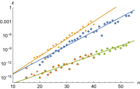
Figure 1: The relative error $\varepsilon=(\hat{p}-p)/p$ versus $n$ for double precision on single-core jobs (upper set of points), double precision on multi-core and multi-node jobs (middle set of points) and double-quadruple precision on single- and multi-core and multi-node jobs (lower set of points). Matrix is $\mathbf{J}$ (see text). From the fitted lines we obtain the decimal digit errors, respectively, $0.37n-17.8$, $0.30n-17.2$ and $0.20n-18$.

II.3 Running time

In Fig. 2 we show the total core time for computing the permanent of an $n\times n$-matrix using the double-quadruple precision approach. The lower set of points ($3\leq n\leq 40$) are for single-core and the upper set of points ($20\leq n\leq 53$) are for multi-core single- and multi-node. For the smaller $n$ we obviously had to repeat the calculation many times to get an estimate of the rather small running times. The almost constant run-time between $20\leq n\leq 30$) is due to the overhead time (ca $5$ seconds) for starting the program with MPI. There is of course an overhead time for OpenMP multi-core as well, but this is much smaller. Several nodes are only used from $n=38$, ranging from $2$ up to $400$ nodes for $n=51,52,53$. The black line indicates a core-time of roughly $10^{-9.2}n2^{n}$ seconds.

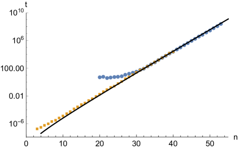
Figure 2: The total core time for a single-core job ($3\leq n\leq 40$, lower set of points, orange squares) and multi-core jobs on one or more nodes ($20\leq n\leq 53$, blue points) for a double-quadruple precision implementation of the permanent. For the multi-core jobs MPI was used for global communication between nodes, thus the overhead time of ca $5$ seconds for $20\leq n\leq 30$. The line corresponds to an estimated run time of $10^{-9.2}n2^{n}$ seconds.

The corresponding plot (not shown) for double-precision is very similar but runs almost twice as fast. The fluctuations between different $n$ is however more pronounced but is not visible in a log-plot. We should mention some effects from, we think, cache memory sizes. For single-core the run time increases, as it should, by a factor slightly larger than $2$. However, at $n=8,16,24,32,40$ this ratio is significantly less than $2$ between $n$ and $n-1$. For example, at $n=8$ the ratio is $0.7$ so it is actually $30\%$ faster to compute an $8\times 8$-permanent than a $7\times 7$-permanent. At $n=16,24,32,40$ the ratio is respectively $1.0$, $1.2$, $1.4$ and $1.6$.

II.4 Improved algorithms for Sparse and Structured Matrices

The basic algorithms for computing the permanent can be modified to handle matrices with many zero entries in a more efficient way, and we will here give a brief discussion of this. As discussed in Ref. Brod (2015) low-depth Boson sampling set-ups lead to sparse matrices, and there it is also proven that under standard complexity theoretic assumptions computing these permanents is exponentially hard even with a constant, but sufficiently large, number of non-zero elements in each row and column. In Ref. Brod (2015) the author suggests that algorithms for this kind of matrix would be of interest and here we demonstrate that they allow for an exponential speed-up over the general case.

The first interesting class is general sparse matrices, i.e., matrices where a significant proportion of the entries are zero. For matrices of this type many of the products in Ryser’s method (3) will be zero, and thus not necessary to compute. If we interpret the matrix $A$ as the adjacency matrix of an edge-weighted graph $G$ we find that a set $J$ can only lead to a non-zero product if $J$ is a dominating set in $G$, i.e., every vertex in $G$ has at least one neighbor in $J$.

If we restrict Eq. (3) to sets $J$ which are dominating sets we still have an exponential time algorithm, but running in time poly$(n)a^{n}$, where $a$ can be noticeably smaller than 2. Listing the minimal dominating sets of $G$ is itself an exponentially hard problem, which can be solved in time $\mathcal{O}(1.7159^{n})$ Fomin et al. (2008). However, for sufficiently sparse graphs we can instead use some simple heuristics which lead us to include both all dominating sets and some non-dominating ones, and still get a significant speed-up compared to the basic version of Ryser’s method. In the sparse version of our code we have implemented this by greedily, according to vertex degree, picking a set of vertices $I$ with disjoint neighborhoods and then listing all subsets $J$ which contains at least one neighbor for every vertex in $I$.

For matrices leading to a sparse graph $G$ we can also prove that the number of dominating sets is exponentially smaller than $2^{n}$, leading to an exponential speed-up over the basic version of Ryser’s formula. We say that a matrix is $d$-sparse if each row and column contains at most $d$ non-zero entries.

Theorem 1.

Let $A$ be a $d$-sparse $n\times n$ matrix. Then the permanent of $A$ can be computed in time

$$\mathcal{O}(n2^{n}(1-2^{-d})^{n/d^{2}})$$

We will return to this theorem and give a proof in Appendix B.

In Fig. 3 we show how the running time increases with $n$ in our Fortran implementation. Clearly this allows for computation of the permanent of surprisingly large matrices. However, with this implementation the improvement quickly vanishes with densities above $5$%, a more ambitious algorithm would surely improve considerably on this.

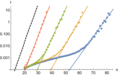
Figure 3: The median run time in seconds for the sparse matrix algorithm for real matrices. Matrices have $1$ on the diagonal (identity matrix) to guarantee a positive permanent. The off-diagonal entries are $1$ with probability $p$ and $0$ with probability $1-p$. From left to right: standard algorithm for dense matrices (black dashed curve), $p=0.05$ (orange triangles), $p=0.02$ (green diamonds), $p=0.01$ (yellow squares) and $p=0.005$ (blue points). The lines have slope $\ln(2)\approx 0.693$, $0.693$, $0.567$, $0.459$ and $0.368$ (left to right).

The associated graph $G$ can also be used to describe the second class of matrices for which we have improved algorithms, namely those for which $G$ has bounded tree-width. This direction is a classical topic Courcelle et al. (2001) and it is well known that for matrices with tree-width bounded by some number $k$ the permanent can be computed in time which is exponential in $k$ but polynomial in $n$. After the first such algorithms a number of improvements have been made Flarup et al. (2007); van Rooij et al. (2009); Meer (2011); Cifuentes and Parrilo (2016), but we are not aware of any efficient implementations of the general bounded tree-width methods. However, one interesting subclass of this family is the set of matrices of limited bandwidth $k$, i.e., matrices $A$ where $a_{i,j}=0$ whenever $|i-j|>k$, for which we can give a practically useful algorithm. This class of matrices is of particular interest in connection with Boson sampling, since they include the unitary matrices for Boson systems with certain restrictions.

For matrices of bandwidth $k$ we can interpret the product in Eq. (1) as a directed walk on the associated graph $G$ where every vertex has out-degree one and in-degree one, and when the bandwidth is limited to $k$ every vertex is connected to only vertices which differ by at most $k$ from its own index $i$. This means that the sums over these weighted paths can be done using a transfer matrix, following the general set up described in Refs. Lundow (2001); Lundow and Markström (2008); Friedland et al. (2010), leading to an algorithm which runs in time $\mathcal{O}(n^{2}2^{k})$, and can in fact be reduced to linear time, in $n$, for fixed $k$. We describe a linear time version of this method in Appendix C.

We have implemented the band-limited method in Mathematica and in Fig. 4 we display the run times for $n\leq 100$ and $k=1,2,3,4,5$ for random real gaussian matrices. Our Mathematica code is available online and this method will be included in an updated Fortran package as well.

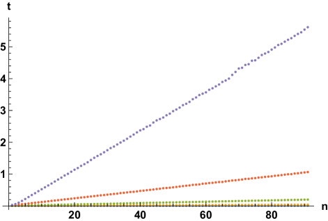
Figure 4: The mean run time in seconds for the bandwith limited algorithm, for matrices with real Gaussian entries for bandwidth, $k=1,\ldots,5$ (upwards in figure), and $n\leq 100$.

For matrices of logarithmic bandwidth this algorithm retains a polynomial run time, but with a degree which depends on the scaling of the logarithm. From the above we then get the following proposition.

Proposition 1.

For $n\times n$ matrices of bandwidth $k\leq c\log n$ the permanent can be computed in time $O(n^{2+c})$.

For a 2-dimensional Boson sampling system where each beam splitter only interacts with its nearest neighbours, or more generally those within some fixed distance $r$, the related unitary matrix will have limited bandwidth. Here the bandwidth depends linearly on both $r$ and the depth of the optical network. As discussed in, e.g., Refs. Jozsa (2006); Clifford and Clifford (2018) these systems can be simulated in sub-exponential time. As long as the input and output states of such a network do not have several photons in a given mode, so called collision free states, the relevant matrix will be of limited bandwidth and our linear time algorithm can be applied. If there are collisions in the output the matrix will have repeated columns and the matrix will still have limited band width as long as the number of collisions is bounded, but the number of collisions now add to the bandwidth. However, note also that if we only have repeated columns our transfer matrix based algorithm can be modified to handle this generalized version of band-limited matrices. Here the ”width” will then instead correspond to the maximum number of non-zero elements in a column.

Observation 1.

Using the algorithm for band-limited matrices as a subroutine the algorithm from Ref. Neville et al. (2017) simulates band-limited Boson sampling systems in polynomial time as long as the number of collisions in the output state is bounded.

For a Haar random unitary the caveat on bounded collisions is not required, due to the Bosonic birthday paradox Arkhipov and Kuperberg (2012); Spagnolo et al. (2013), which guarantees that collisions will be unlikely if the number of Bosons is not too large. For low-depth systems this theorem does not apply, but due to the bounded range of the interactions we still do not expect large numbers of collisions in a single output mode for a random input state. Providing an exact quantitative form of this statement, converging to the Bosonic birthday paradox as depth increases, would be of interest.

III Complex Gaussian matrices

Let $A=(a_{i,j})$ be an $n\times n$-matrix of i.i.d. complex Gaussian numbers, i.e., $A$ is a member of the Ginibre ensemble $\mathcal{G}(n)$. Each element $a_{i,j}$ can be generated by first producing two independent real Gaussian numbers $g_{1}$ and $g_{2}$, using the Box-Muller method Box and Muller (1958), and then $(g_{1}+\imath g_{2})/\sqrt{2}$ is a random complex Gaussian with mean 0 and variance $1$. Clearly, the expected value of the permanent of a matrix with such entries is $0$, due to symmetry. However, we are mainly interested in the properties of the modulus $|\operatorname{per}(A)|$. It is known Aaronson and Arkhipov (2013) that $\left\langle|\operatorname{per}(A)|^{2}\right\rangle=n!$, and this is true as long as the entries are independent real or complex numbers with variance 1, so that it is more natural to work with the random variable $X=|\operatorname{per}(A)|/\sqrt{n!}$ and thus have $\left\langle X^{2}\right\rangle=1$.

Remarkably, it is also shown in Ref. Aaronson and Arkhipov (2013) that $\left\langle X^{4}\right\rangle=n+1$. In general, the authors of Ref. Aaronson and Arkhipov (2013) can express the even moments exactly in terms of the expected number of decompositions of a $k$-regular multigraph into disjoint perfect matchings. An asymptotic result, following from the proof of van der Waerden’s conjecture on the permanent of doubly-stochastic matrices, is then that $\left\langle X^{2k}\right\rangle\sim(k/e)^{n}$ for $k\geq 3$.

We will denote the distribution function by $F(x,n)=\Pr(X\leq x)$ where $X$ are samples from $n\times n$-matrices. The density function is denoted $f(x,n)=F^{\prime}(x,n)$. Also let $f(x)=f(x,\infty)$ and $F(x)=F(x,\infty)$ but we also use $f(x)$ and $F(x)$ as generic forms when the context is clear. The $x$-values are chosen in a geometric progression of $16$ per decade (an interval of the form $[10^{k-1},10^{k})$ for some integer $k$). The density $f(x,n)$ is then obtained from the difference quotient $f(x_{i})=(F(x_{i+1})-F(x_{i-1}))/(x_{i+1}-x_{i-1})$. The error in $F(x)$ is estimated as $\epsilon(x)=\sqrt{F(x)\,(1-F(x)}/\sqrt{m}$ where $m$ is the number of samples. The error in $f(x)$ can then be obtained in the usual fashion.

III.1 Measuring up the distribution

For each size $n$ we have computed the permanent of $10^{6}$ random complex Gaussian $n\times n$-matrices, for $n=1,2,\ldots,30$, which we will use in this section, and $10^{5}$ matrices for $n=31,\ldots,35$, to be used later. Let us take a look at the moments $\left\langle X^{k}\right\rangle$ of the sampled data. In Fig. 5 we show the mean $\left\langle X\right\rangle$ vs $1/n$. A fitted line suggests the limit mean value $0.684(1)$ where the error estimate is obtained from fitting on the points $n\geq k$ with $k=6,\ldots,12$. The error bars in the figure were estimated from bootstrap resampling. For the second moment, shown in Fig. 6, we know that it should be $1$ and indeed there is only noise-like deviation from the line $y=1$.

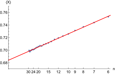
Figure 5: Gaussian entries. Mean value $\left\langle X\right\rangle$ versus $1/n$ for $n=6,7,\ldots,30$ and the fitted line $y=0.684+0.42x$ (red) where $x=1/n$.

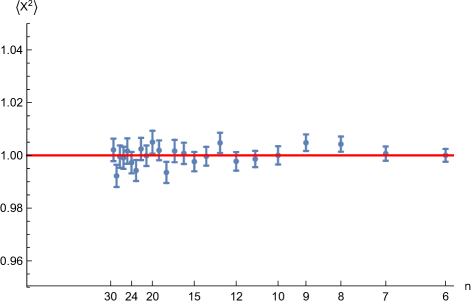
Figure 6: Gaussian entries. Mean value $\left\langle X^{2}\right\rangle$ versus $1/n$ for $n=6,7,\ldots,30$ and the line $y=1$.

In Fig. 7 the third moment is shown and the noise is still manageable. Using the line fitting procedure described for the first moment, suggests the limit $3.20(3)$. In Fig. 8 we show the fourth moment $\left\langle X^{4}\right\rangle$, which should be $n+1$, plotted against $n$. A line $y=1+x$ together with the data points indicate that for larger $n$ the data often favor a smaller moment. However, the error bars occasionally get quite pronounced. This indicates that our data set, from lack of samples, has not yet fully explored the rather heavy tails of the distribution.

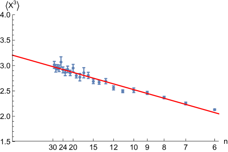
Figure 7: Gaussian entries. Mean value $\left\langle X^{3}\right\rangle$ versus $1/n$ for $n=6,7,\ldots,30$ and the line $3.20-6.8x$ (red) where $x=1/n$.

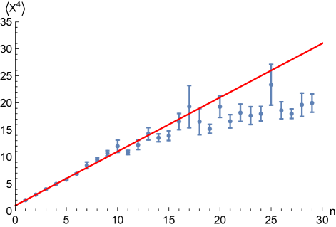
Figure 8: Gaussian entries. Mean value $\left\langle X^{4}\right\rangle$ versus $n$ for $n=1,2,\ldots,30$ and the line $y=1+n$ (red), i.e. the correct expected value.

Finally, in Fig. 9 we show the distribution density for $n=30$. This brings us to an interesting conjecture; the permanent anti-concentration conjecture, see Ref. Aaronson and Arkhipov (2013). It states that there exists a polynomial $p$ such that

$$F(1/p(n,1/\delta))<\delta$$ (5)

for all $n$ and $\delta>0$. Equivalently, this can be formulated as the existence of constants $a$, $b$, $c$ such that

$$F(\varepsilon)<cn^{a}\varepsilon^{b}$$ (6)

for all $n$ and $\varepsilon>0$. In the next section we will provide numerical support for this conjecture.

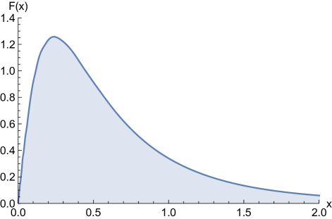
Figure 9: Gaussian entries. Density function $f(x)$ versus $x$ for $n=30$. Data from $10^{6}$ random $30\times 30$-matrices $A$. This range ($x<2$) contains $95$% of the samples.

III.2 The distribution in detail

Let us try to discern how $F(x)$ behaves for small $x$. In Fig. 10 we show $F(x,n)$ for $n=6,\ldots,30$ for a few values of $x$ together with fitted lines. It turns out that $F(x,n)$ depends quite linearly on $1/n$ for $n\geq 6$. When smaller $n$ are included a higher-order correction term becomes necessary. Note that $F(x,n)$ is strictly increasing with $n$ for $x\lesssim 1.77$. For each fixed $x$ we fit a line through the points $(1/n,F(x,n))$ and its constant term then gives us an estimated asymptotic value, i.e. we make the ansatz $F(x,n)=F(x)+C(x)/n$ so that the slope $C(x)$ only depends on $x$. By deleting individual points from the line fitting we obtain error estimates of the parameters of each line. At $x\lesssim 0.005$ the probabilities become less than $10^{-4}$ and the error bar for each estimate of $F(x)$ becomes significant. We have thus only used $x\geq 0.005$.

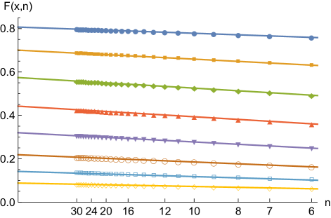
Figure 10: Gaussian entries. $F(x,n)$ for $n=6,\ldots,30$ at $x=1$, $0.75$, $0.56$, $0.42$, $0.32$, $0.24$, $0.18$ and $0.13$ (downwards). Lines are fitted to each set of points. Error bars are smaller than the points.

In Fig. 11 we show a log-log plot of the asymptotic $F(x)$. We have fitted a line with slope $2$ through the points $x<0.05$ which corresponds to the approximation $F(x)\sim 6.0(1)x^{2}$. The lower inset of the figure shows the ratio $F(x)/x^{2}$ which plausibly approaches the limit $6$ despite some significant noise beginning for $x\lesssim 0.01$. The upper inset of Fig. 11 shows a log-log plot of the difference $6x^{2}-F(x)$ approximated by $7(1)x^{3}$ (note the rather wide error bar), as indicated by the red line having slope $3$. Together they suggest $F(x)\sim 6x^{2}-7x^{3}$. The error estimates captures how sensitive the coefficients are to deleting data for individual $n$ and which interval of $x$ we fit lines to.

There is also the matter of finite-size scaling to take into account, i.e., the $n$-dependence. A similar analysis of the slopes of the lines in Fig. 10, i.e., the parameter $C(x)$ mentioned above, gives that $C(x)\sim-12.0(5)x^{2}$. Including the finite-size term we then have the finite-size scaling

$$F(x,n) \sim \left(6-\frac{12}{n}\right)x^{2}-7x^{3},$$ (7)

$$f(x,n) \sim \left(12-\frac{24}{n}\right)x-21x^{2}$$ (8)

In the next subsection we will try to obtain a finite-size correction for the $x^{3}$-term. In any case, we have so far found that $F(x)\lesssim 6x^{2}$ for all $n$ and $x$ which supports that the anti-concentration conjecture is true.

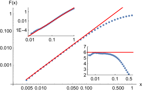
Figure 11: Gaussian entries. Log-log plot of $F(x)$ and the line (red) corresponding to the approximation $6x^{2}$ (see text). The upper inset shows a log-log plot of $6x^{2}-F(x)$ and a line (red) corresponding to $7x^{3}$. The lower inset shows the ratio $F(x)/x^{2}$ and the line (red) is at $y=6$.

III.3 The distribution of the squares

Let us now see how this translates to the distribution of the squares $X^{2}$. The distribution function of $X^{2}$ is $F_{2}(x)=\Pr(X^{2}\leq x)=\Pr(X\leq\sqrt{x})=F(\sqrt{x})$. This gives the density function $f_{2}(x)=F^{\prime}_{2}(x)=f(\sqrt{x})/(2\sqrt{x})$. Using Eq. (7) and Eq. (8) we obtain

$$F_{2}(x) \sim \left(6-\frac{12}{n}\right)x-7x^{3/2}$$ (9)

$$f_{2}(x) \sim 6-\frac{12}{n}-10.5\sqrt{x}$$ (10)

In Fig. 12 we show the density function $f_{2}(x,n)$ of $X^{2}$ for $n=30$. It was speculated in Ref. Aaronson and Arkhipov (2013) that the density $f_{2}(x)$ goes to infinity when $x\to 0$ but we claim that it goes to a limit value. Our approximation for $F(x)$ stays relevant for $x\lesssim 0.10$ which from the perspective of the squares $X^{2}$ means that our formula for $f_{2}(x)$ is relevant only for $x<0.01$. We are here at the lower $5$% of our data set so our analysis demands a large number of samples.

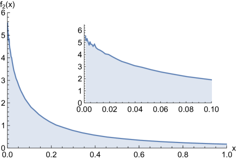
Figure 12: Gaussian entries. Distribution density $f_{2}(x,30)$ of $X^{2}$ for $n=30$. The shown range covers $80\%$ of the samples. The inset shows a zoomed-in version convering $30\%$ of the samples.

Fitting the curve $y=C_{0}+C_{1}\sqrt{x}$ to the measured $f_{2}(x,n)$ for the range $0.0005<x<0.01$ we find how the coefficients $C_{0}$ and $C_{1}$ depend on $n$. Note that $C_{0}$ should scale as $C_{0}=6.0(1)-12.0(5)/n$ as in Eq. (10). This is confirmed in Fig. 13. The inset shows how $C_{1}$ depends on $n$ and we find $C_{1}=10.5(9)+36(6)/n$ though the points are here quite scattered, which is reflected in the error bars. Again, the error bars indicate how much the result depends on the choice of fitted points (less) and range (more).

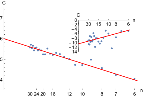
Figure 13: Gaussian entries. Scaling of the coefficients $C_{0}$ and $C_{1}$ (inset) for $f_{2}(x,n)=C_{0}+C_{1}\sqrt{x}$ fitted to $0.0005<x<0.01$. The red lines are $y=6-12/n$ and $y=-10.5+36/n$ (inset).

Adding these new terms we find the following finite-size scaling rules

$$F(x,n) \sim \left(6-\frac{12}{n}\right)x^{2}+\left(-7+\frac{24}{n}\right)x^{3},$$ (11)

$$f(x,n) \sim \left(12-\frac{24}{n}\right)x+\left(-21+\frac{72}{n}\right)x^{2},$$ (12)

$$F_{2}(x,n) \sim \left(6-\frac{12}{n}\right)x+\left(-7+\frac{36}{n}\right)x^{3/2},$$ (13)

$$f_{2}(x,n) \sim 6-\frac{12}{n}+\left(-10.5+\frac{36}{n}\right)\sqrt{x}$$ (14)

with the limits

$$F(x) \sim 6x^{2}-7x^{3}$$ (15)

$$f(x) \sim 12x-21x^{2}$$ (16)

$$F_{2}(x) \sim 6x-7x^{3/2}$$ (17)

$$f_{2}(x) \sim 6-10.5\sqrt{x}$$ (18)

In Fig. 14 we show the measured $f(x,n)$ and the function in Eq. 12 for $n=10,20,30$ on $x<0.1$. The fit is quite excellent. In Fig. 15 we show the measured $f_{2}(x,n)$ and Eq. (14) for $x<0.008$, again with a good fit though the error bars for $f_{2}$ are here quite noticeable.

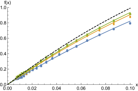
Figure 14: Gaussian entries. Measured density $f(x,n)$ (points) and the scaling rule of Eq. (12) for $n=10,20,30$ (blue, orange, green curves; upwards) and $\infty$ (dashed black curve). Error bars are smaller than the points.

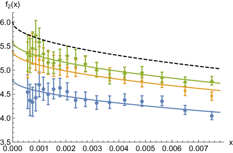
Figure 15: Gaussian entries. Measured density $f_{2}(x,n)$ (points) and the scaling rule of Eq. (14) for $n=10$, $20$, $30$ (blue, orange, green curves; upwards) and $\infty$ (dashed black curve). Error bars become significant for $x\lesssim 0.001$.

IV Complex circular distribution

Here we let the entries of the matrix be random complex numbers of modulus $1$, i.e. we let each entry be of the form $\exp(\imath\theta)$ where $\theta$ is uniformly distributed on the interval $[0,2\pi)$. For each size $n$ we have collected data for $10^{7}$ such random matrices, for $n=1,2,\ldots,30$. As before, we study the distribution of $X=|\operatorname{per}{A}|/\sqrt{n!}$. Our investigation proceeds as in the previous section though we are here armed with better data.

The mean $\left\langle X\right\rangle$ is shown in Fig. 16 and from fitted 2nd degree polynomials we estimate the limit $0.7753(2)$. The second moment is again exactly $1$ but obviously we see some small fluctuations. The behaviour is quite similar to that in Fig. 6 but with less noise. The third moment $\left\langle X^{3}\right\rangle$ in Fig. 17 prefers the limit $2.41(2)$, as per fitted polynomials as before. The fourth moment $\left\langle X^{4}\right\rangle$, shown in Fig. 18, has a linear behavior just as for the Gaussian case in Fig. 8. A rough estimate of its behavior, based on $n\leq 13$, is $\langle X^{4}\rangle\sim 0.72(2)+0.37(1)n$.

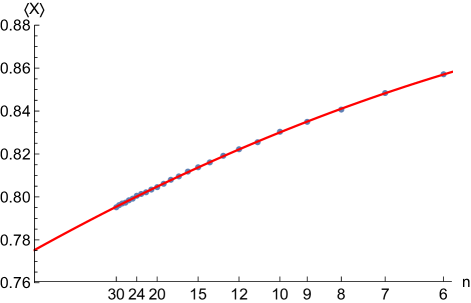
Figure 16: Complex circular entries. Mean value $\left\langle X\right\rangle$ versus $1/n$ for $n=6,7,\ldots,30$ and the fitted polynomial $y=0.7753+0.634x-0.862x^{2}$ where $x=1/n$. Error bars are smaller than the points.

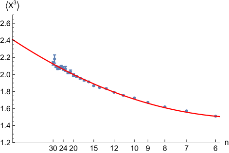
Figure 17: Complex circular entries. Mean value $\left\langle X^{3}\right\rangle$ versus $1/n$ for $n=6,7,\ldots,30$ and the fitted polynomial $y=2.41-9.4x+24x^{2}$.

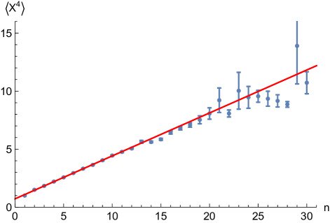
Figure 18: Complex circular entries. Mean value $\left\langle X^{4}\right\rangle$ versus $n$ for $n=1,2,\ldots,30$ and the line $y=0.72+0.37n$.

The distribution density $f(x)$ looks very similar to that of the Gaussian case. To estimate the limit distribution function $F(x)$ we use the ansatz $F(x,n)=C_{0}+C_{1}(x)/n+C_{2}(x)/n^{2}$ on the points $n\geq 5$. Note that the linear ansatz used in the Gaussian case is not sufficient here. In Fig. 19 we show a log-log plot of the limit $F(x)$. The red line has slope $2$ so again we expect $F(x)\propto x^{2}$ for small $x$. The inset shows the ratio $F(x)/x^{2}$ and, despite the noise setting in at $x<0.01$, we estimate $F(x)/x^{2}\sim 2.135(10)$. The error bar includes both errors from excluding points in the $F(x,n)$ ansatz and errors depending on which points $x$ to include (we have used $0.01\leq x\leq 0.08$). Clearly, as shown by the inset figure, the rule $F(x)\sim 2.135x^{2}$ breaks down for $x\gtrsim 0.1$. Including the finite-size scaling we find the following rule useful for $x\leq 0.1$ for $n\geq 5$:

$$F(x,n)\sim\left(2.135-\frac{8}{n}+\frac{15}{n^{2}}\right)\,x^{2}$$ (19)

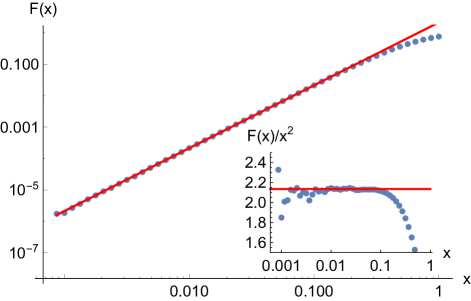
Figure 19: Complex circular entries. Log-log plot of limit $F(x)$ versus $x$ for $x\leq 0.1$. The red line, having slope $2$, corresponds to the approximation $F(x)\sim 2.135x^{2}$. The inset shows $F(x)/x^{2}$ versus $\log x$ and the red line is the constant $y=2.135$. Noise becomes noticable for $x\lesssim 0.01$.

Information on higher order terms are easier found when studying the distribution of the squares. The distribution in Eq. (19) translates to $f_{2}(x,n)=2.135-8/n+15/n^{2}$ so that the limit density is just the constant $2.135$ for, say, $x\lesssim 0.01$. However, plotting $f_{2}(x,n)$ reveals that the density functions are very close to linear for $x\lesssim 0.1$ and all $n\geq 5$. Using the simple ansatz $f_{2}(x,n)=C_{0}+C_{1}x/n$ and fitting on the interval $0.005\leq x\leq 0.08$ we find that the slope scales as $C_{1}=-6.0(2)+46(3)/n-110(20)/n^{2}$ where the error bars mainly indicate sensitivity to which points are included. Note that the constant coefficient must scale as $C_{0}=2.135-8/n+15/n^{2}$, see Eq. (19). To conclude, after defining the coefficients

$$C_{0} = 2.135-\frac{8}{n}+\frac{15}{n^{2}}$$ (20)

$$C_{1} = -3+\frac{23}{n}-\frac{55}{n^{2}}$$ (21)

we obtain the finite-size scaling rules

$$F(x,n) \sim C_{0}\,x^{2}+C_{1}\,x^{4}$$ (22)

$$f(x,n) \sim 2C_{0}\,x+4C_{1}\,x^{3}$$ (23)

$$F_{2}(x,n) \sim C_{0}\,x+C_{1}\,x^{2}$$ (24)

$$f_{2}(x,n) \sim C_{0}+2C_{1}\,x$$ (25)

and their respective limits become

$$F(x) \sim 2.135x^{2}-3x^{4}$$ (26)

$$f(x) \sim 4.27x-12x^{3}$$ (27)

$$F_{2}(x) \sim 2.135x-3x^{2}$$ (28)

$$f_{2}(x) \sim 2.135-6x,$$ (29)

In Figs. 20 and 21 we compare the rules for $f(x,n)$ and $f_{2}(x,n)$ to their measured counterparts. They fit very well over a surprisingly wide interval. Translating the limit $f_{2}(x)=2.135-6x$ to $F(x)$ we find $F(x)=2.135x^{2}-3x^{4}$ which adds a correction term to Eq. (19). Note that in Eq. (26) this correction term is of order $x^{4}$ whereas it was of order $x^{3}$ in the Gaussian case.

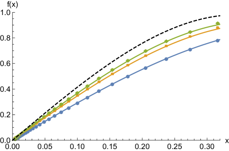
Figure 20: Complex circular entries. Measured density $f(x,n)$ (points) and the scaling rule of Eq. (23) for $n=10$, $20$, $30$ (blue, orange, green curves; upwards) and $\infty$ (dashed black curve). Error bars are smaller than the points.

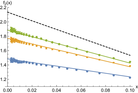
Figure 21: Complex circular entries. Measured density $f_{2}(x,n)$ (points) and the scaling rule of Eq. (25) for $n=10$, $20$, $30$ (blue, orange, green curves; upwards) and $\infty$ (dashed black curve).

V Bernoulli-distributed entries

We will here apply the approach in the previous section to a discrete class of random matrices, that of Bernoulli-distributed $\pm 1$ entries where $\Pr(+1)=\Pr(-1)=1/2$. Matrices with Bernoulli-distributed entries have been studied in the mathematics literature, with an emphasis on the probability for small values of $X$. In Tao and Vu (2009) it was proven that with probability tending to 1 $X$ is larger than $n^{(n/2-\epsilon)}$ for any fixed $\epsilon>0$, and that it is likewise smaller than $n^{(n/2+\epsilon)}$ with probability tending to 1. Those authors also conjectured that the lower bound can be improved to $\exp(-cn)n^{n/2}$ for some constant $c$, and we will comment more on this later.

Our data consists of $10^{6}$ samples for $n=1,2,\ldots,30$. Unfortunately we can not obtain quite the same level of precision in our scaling analysis as for the complex Gaussian and circular cases. Strong finite-size effects and erratic behavior for smaller $n$ calls for larger matrices and many more samples.

Starting out with the first moment $\left\langle X\right\rangle$ in Fig. 22 we find that it is asymptotically $0.647(2)$. The second moment is of course $1$ and the third moment is asymptotically $3.75(5)$ (not shown). The fourth moment, as in the Gaussian case, appears to grow linearly with $n$ but we only give the very rough estimate $\left\langle X^{4}\right\rangle\approx 1.25(5)n-1.0(5)$ due to its erratic behavior.

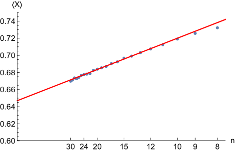
Figure 22: Bernoulli entries. Mean value $\left\langle X\right\rangle$ versus $1/n$ for $n=8,9,\ldots,30$ and the line $y=0.647+0.73x$ (red) where $x=1/n$. Error bars are smaller than the points.

In Fig. 23 we show a log-log plot of $F(x)$ plotted versus $\log x$ where $F(x)$ was obtained using a similar finite-size scaling ansatz as in the previous cases. However, we note here that care must be taken to only include matrices large enough since the corrections-to-scaling are considerably larger in this case. We have only used $n\geq 15$ which contributes some noise to the estimated $F(x)$ since we fit on fewer points. The red line in Fig. 23 has slope $1$ and corresponds to the estimate $F(x)\sim 1.33(5)x$. The inset shows the ratio $F(x)/x$ which is clearly approaching a limit around $1.33(5)$.

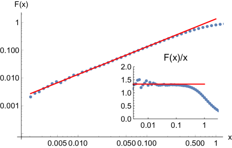
Figure 23: Bernoulli entries. Log-log plot of $F(x)$ and a line with slope $1$ (red) corresponding to the approximation $F(x)\sim 1.33x$. The inset shows the ratio $F(x)/x$ versus $\log x$ together with the line $y=1.33$ (red).

Unfortunately our data are not good enough for a correction term of higher order and pin-pointing the finite-size scaling would also be an unreliable affair. We will simply translate our distribution function into the distribution of $X^{2}$. In conclusion we thus find the asymptotes

$$F(x) \sim 1.33x$$ (30)

$$f(x) \sim 1.33$$ (31)

$$F_{2}(x) \sim 1.33\sqrt{x}$$ (32)

$$f_{2}(x) \sim 0.665/\sqrt{x}$$ (33)

Note here that we claim that $f_{2}(x)\to\infty$ when $x\to 0$ unlike for the complex Gaussian and circular cases where $f_{2}(x)$ approached a limit of $6.0(1)$ and $2.135(10)$ respectively. In Fig. 24 we show the measured $f(x,n)$ (inset) and $f_{2}(x,n)$ for $n=30$ and compare them to the limits of Eq. (31) and (33).

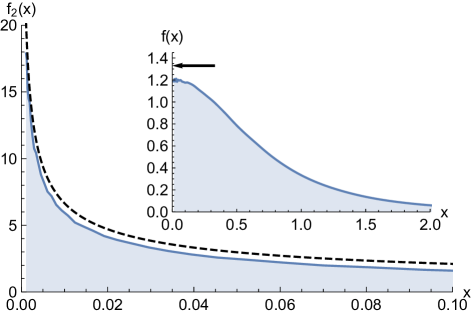
Figure 24: Bernoulli entries. Measured density of $X^{2}$ for $n=30$, i.e. $f_{2}(x,30)$, and the estimated limit $f_{2}(x)=0.665/\sqrt{x}$ (dashed black curve). The inset shows the measured density of $X$ for $n=30$, i.e. $f(x,30)$. The black arrow indicates the limit $f(x)=1.33$.

Finally we note that our data is compatible with a strengthening of the conjecture from Tao and Vu (2009)

Conjecture 1.

$X$ is asymptotically almost surely larger than

$$h(n)\exp(-n/2)n^{(n/2+1/4)},$$

where $h(n)$ is any function tending to 0 as $n\rightarrow\infty.$

VI Gaussian behaviour of minors of unitary matrices

The computational hardness of Boson sampling as analysed in Aaronson and Arkhipov (2013) depends on the fact that certain submatrices of Haar-random unitary matrices asymptotically behave like random matrices with Gaussian entries. Next we will investigate how close the permanent of such a submatrix is to the permanent of a random Gaussian matrix.

Let $\mathcal{U}(n)$ be the family of unitary $n\times n$-matrices. We can generate random members of $\mathcal{U}(n)$ under the Haar-measure in the following way Mezzadri (2007); produce a complex random Gaussian matrix $A$ as above, find its QR-decomposition with $R=(r_{i,j})$, let $\Lambda=(\lambda_{i,j})$ be the diagonal matrix of normalized elements of $R$ so that $\lambda_{i,j}=\delta_{i,j}r_{i,j}/|r_{i,j}|$ (where $\delta_{i,j}$ is the Kronecker delta), then $U=Q\Lambda$ is a random unitary matrix from $\mathcal{U}$.

Now let $\mathcal{S}(m,n)$ be a family of random matrices obtained by first generating a random unitary $m\times m$-matrix $U\in\mathcal{U}(m)$, next let $U_{n}$ be the top-left $n\times n$-submatrix of $U$ and set $S=\sqrt{m}U_{n}$. Then $S$ is a random matrix from the family $\mathcal{S}(m,n)$.

It is known that if $S\in\mathcal{S}(n^{6},n)$ and $A\in\mathcal{G}(n)$ then the variation distance between them is expected to be small, i.e., they have essentially the same probability distribution. The authors of Ref. Aaronson and Arkhipov (2013) prove a slightly stronger result but they also think $n^{6}$ can be replaced by something much smaller, say closer to $n^{2+\epsilon}$. We will use distributions of the permanent to see if we can throw some light on the problem.

We will use the Kolmogorov-Smirnov (KS) statistic $D=\sup_{x}|F(x)-G(x)|$ as a measure of the distance between two empirical distribution functions $F(x)$ and $G(x)$. For a two-sample test, we reject the null hypothesis that they are the same (at significance level $\alpha$) if $D>D_{\alpha}$ for certain $D_{\alpha}$. For $\alpha=0.05$ and using $10^{5}$ samples for both distributions we get $D_{\alpha}=0.00607$. We then first generate $S\in\mathcal{S}(n^{a},n)$ and compute $|\operatorname{per}(S)|/\sqrt{n!}$ for $10^{5}$ different $S$ and then compare this distribution to that of $|\operatorname{per}(A)|/\sqrt{n!}$ for $10^{5}$ complex Gaussian matrices $A$. We will see if the distance $D$ has an increasing or decreasing trend for different values of $a$. Note that when $n^{a}$ is not an integer we just round to the nearest integer. We use Mathematica’s built-in routine for computing the test statistic when comparing two distributions in a Kolmogorov-Smirnov test as the value of $D$.

We have run this test for $5$ different $a$ and a wide range of $n$ for each $a$: $1\leq n\leq 34$ for $a=2$, $1\leq n\leq 32$ for $a=2.25$, $1\leq n\leq 30$ for $a=2.50$, $1\leq n\leq 22$ for $a=2.75$ and $1\leq n\leq 17$ for $a=3$. In Fig. 25 we show the KS-statistic $D$ versus $n\geq 3$ for the different $a$.

For $a=2$ the values of $D$ are clearly increasing at first but there is no clear trend beginning at $n\approx 28$, with $D$ staying at roughly $0.08$. For $a=2.25$ there is a very weak increasing trend in $D$. Excluding individual points from the line fit is not enough to get a decreasing trend though. For $a=2.5$ there is a distinctly decreasing trend but it would take $n\approx 75$ to pass a KS-test at the $5$% level. For $a=2.75$ the distributions actually pass a KS-test for $n=19$, $21$, $22$ and for $a=3$ they pass it for $n=12$ and $13$.

Reading the trends in the KS-statistic $D$, it would thus appear that matrices from $\mathcal{S}(n^{a},n)$ are essentially indistinguishable from complex Gaussian $n\times n$-matrices, in terms of their permanents, when $a>2.25$, while for $a<2.25$ they are not, and the case of $a=2.25$ appears to be a separator between the two cases which we cannot classify. If this is a correct classification, rather than an effect of slow convergence in terms of $n$ for the lower values of $a$, then it would contradict the conjecture in Ref. Aaronson and Arkhipov (2013) that $a\geq 2+\epsilon$ is enough.

It is possible that the curve for $a=2$ will begin to decrease for larger $n$, in accordance with the conjecture from Ref. Aaronson and Arkhipov (2013). Nontheless, for $a<2.25$, we see a behaviour which is distinct from the Gaussian case for the range of $n$ used here. So, care must be taken in the analysis of Boson sampling experiments where an effective value of $a$ close to, or equal to, 2 has been chosen if the number of Bosons is small.

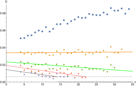
Figure 25: KS-statistic $D$ plotted versus $n$ for the five different $a$. Downwards in figure are data sets for $a=2.00$ (blue points), $2.25$ (orange squares), $2.50$ (green diamonds), $2.75$ (pink up-triangles) and $3.00$ (purple down-triangles). Both distributions are based on $10^{5}$ samples so $D_{0.05}=0.00607$ (dashed line). The fitted lines are $0.034+0.000031x$ for $a=2.25$, $0.023-0.00031x$ for $a=2.50$, $0.019-0.00060x$ for $a=2.75$ and $0.014-0.00058x$ for $a=3$.

VII Conclusions

In order to compute output probabilities for Boson sampling experiments Aaronson and Arkhipov (2013) one has to compute the permanent of the associated unitary matrices. Here we have presented a software package for doing such computations efficiently, both on serial and parallel machines. Our programs are efficient enough to allow us to beat the previous world record for computation of permanents in a substantial way, despite the fact that the previous record was set on a far larger cluster Wu et al. (2018).

Our package also has specialised functions for matrices of limited bandwidth, running in time $\mathcal{O}(2^{k}n^{2})$ for matrices of bandwidth $k$, and in linear time for fixed $x$. This makes it possible to classically simulate a Boson sampling system of depth $\mathcal{O}(\log{n})$ in polynomial time

We have used our software package to perform a large scale simulation study of the anti-concentration conjecture for permanents Aaronson and Arkhipov (2013). Here we find that the conjecture agrees well with the conjecture, both for complex Gaussian matrices and other matrix classes. We also investigated how well the permanent of a minor of size $n^{a}$ of an $n\times n$ Haar-random unitary matrix can be approximated by the permanent of a random Gaussian matrix. Here we find some possible tension with the most optimistic version of a conjecture from Ref. Aaronson and Arkhipov (2013).

Appendix A A parallel version of Ryser’s algorithm

We here collect the algorithms necessary for computing the permanent of general matrices on a parallel computer. Fortran and Mathematica implementations can be freely downloaded and used from our website Lundow and Markström (2019).

Distributing the computation equally on a number of nodes is of course easily done. The computation is a sum with $2^{n-1}$ terms and we only need to split the sum into equal parts (or as equal as is possible). To distribute a sequence $(r_{0},r_{1},\ldots,r_{n-1})$ as evenly as possible into $m$ subsequences $(s_{0},s_{1},\ldots,s_{m-1})$, where $s_{i}=(r_{k},r_{k+1},\ldots,r_{k+\ell-1})$, we need to find $k$ and $\ell$ for each $i=0,\ldots,m-1$:

• distribute$(n,m,i,k,\ell)$

• In: $n\geq 0$, $m\geq 1$, $0\leq i<m$

• Out: $k$, $\ell$

• $q:=\lfloor n/m\rfloor$

• $r:=n\bmod m$

• $k:=i\cdot q+\min(i,r)$

• $\ell:=q+\mathcal{I}(i<r)$

Here $\mathcal{I}(s)$ is an indicator function returning $1$ if statement $s$ is true and $0$ if $s$ is false.

The sequence in question is of course the Gray-code sequence. To find the first code in a subsequence we need to unrank the Gray-code, i.e. compute the $k$th code $x=(x_{1},x_{2},\ldots)$ in the Gray-code sequence. It is common practice that this is obtained as

$$x:=\mathrm{xor}(k,\mathrm{rshift}(k))$$ (34)

where $\mathrm{xor}$ is the bit-wise exclusive-or function of two integers and $\mathrm{rshift}$ denotes a bit-wise shift of an integer one step to the right.

Computing the next Gray-code in the sequence is also common knowledge, see e.g. Ref. Nijenhuis and Wilf (1978), but we include it here for completeness:

• nextset$(t,j,x)$

• In: $t=\pm 1$ and binary vector $x$.

• Out: integer $j$ and updated $t$ and $x$.

• $j:=1$ (first position of $x$)

• $t:=-t$

• if $t=1$ then

• while $x_{j}=0$ do

• $j:=j+1$

• end do

• $j=j+1$

• end if

• $x_{j}:=1-x_{j}$

The permanent of a $n\times n$-matrix is a sum of $2^{n-1}$ terms which we want to distribute over, say, $m$ nodes (or threads). Each node then computes the partial sum $S_{k}$ for $k=0,1,\ldots,m-1$. For details, see Ref. Nijenhuis and Wilf (1978).

• subpermanent$(A,n,m,k,S)$

• In: $n\times n$-matrix $A=(a_{ij})$, integers $0\leq k<m$.

• Out: partial sum $S$.

• $\mathrm{distribute}(2^{n-1},m,k,r,\ell)$

• $x:=\mathrm{xor}(r,\mathrm{rshift}(r))$ (where $x=(x_{1},x_{2},\ldots,x_{n})$)

• $t:=(-1)^{r}$

• $S:=0$

• for $i=1,2,\ldots,n$ let $w_{i}:=a_{i,n}-\tfrac{1}{2}\sum_{j=1}^{n}a_{i,j}$

• for $j=1,2,\ldots,n-1$ where $x_{j}=1$ do

• for $i=1,2,\ldots,n$ let $w_{i}:=w_{i}+a_{i,j}$

• end do

• do $\ell$ times

• $p:=\prod_{i=1}^{n}w_{i}$

• $\mathrm{nextset}(t,j,x)$

• $S:=S+t\cdot p$

• $z:=2x_{j}-1$

• for $i=1,2,\ldots,n$ let $w_{i}:=w_{i}+z\cdot a_{i,j}$

• end do

Collecting and adding up the partial sums is easy.

• permanent$(A,n,m,S)$

• In: $n\times n$-matrix $A$ and integer $m\geq 1$.

• Out: permanent $S$.

• for $k=0,1,\ldots m-1$ do

• $\mathrm{subpermanent}(A,n,m,k,S_{k})$

• end do

• $S:=2\,(-1)^{n}\,\sum_{k=0}^{m-1}S_{k}$

For completeness we also describe Kahan summation Kahan (1965). Consider the following standard summation loop computing $S:=a_{1}+\cdots+a_{n}$,

• $S:=0$

• for $i=1,2,\ldots,n$ do

• $S:=S+a_{i}$

• end do

In Kahan summation we do instead the following

• $S:=0$

• $b:=0$

• for $i=1,2,\ldots,n$ do

• $c:=a_{i}-b$

• $t:=S+c$

• $b:=(t-S)-c$

• $S:=t$

• end do

Appendix B Algorithm for Sparse Matrices

The main observation behind our improvement for sparse matrices on Ryser’s method comes from the observation that in a sparse matrix many of the products in Ryser’s formula (3) will be zero. By avoiding sets $J$ which are guaranteed to lead to a zero sum in the innermost product we may achieve a speed-up.

If we interpret the matrix $A$ as the adjacency matrix of an edge-weighted graph $G$, where vertices may have loops, we find that a set $J$ can only lead to a non-zero product if $J$ is a dominating set in $G$, i.e., every vertex in $G$ has at least one neighbor in $J$. Finding all dominating sets can be done in exponential time, with a basis smaller than 2 Fomin et al. (2008), but we can instead use a faster approximate algorithm which still leads to a speed-up over the general version of Ryser’s formula.

A subset $S$ of the vertex set of $G$ is domination restricting if every dominating set of $G$ must contain a vertex from $S$. The full vertex set of $G$ is domination restricting, as is the neighourhood of a single vertex. We say that a list of sets $L=(S_{1},S_{2},\ldots,S_{t})$ is domination restricting if each set $S_{i}$ is domination restricting and the sets are pairwise disjoint. We now note that every dominating set $J$ in $G$ must have a non-empty intersection with each set in $L$. So, if we use all sets $J$ with this property we will include all dominating sets $J$, and some sets which may not be dominating, while excluding a potentially large number of sets. Below we give a randomized greedy algorithm for constructing a useful list $L$.

We say that a matrix $A$ is $d$-sparse if every row and column contains at most $d$ non-zero entries. For this type of matrix a good choice of $L$ will lead to an exponential speed-up over the basic version of Ryser’s formula. Let us now re-state and prove the theorem in Sec. II.4.

Theorem 2.

Let $A$ be a $d$-sparse $n\times n$ matrix. Then the permanent of $A$ can be computed in time

$$\mathcal{O}(n2^{n}(1-2^{-d})^{n/d^{2}})$$

Proof.

Let $G^{2}$ be the square of the graph $G$ associated with $A$, i.e. the graph where two vertices are adjacent if they are at distance at most 2 in $G$. The graph $G^{2}$ has degree at most $d^{2}$, so if $n>d^{2}$ we can properly colour the vertices of $G^{2}$ using $d^{2}$ colours.

Now we can construct a domination restricting list $L$ by taking a colour class of size at least $n/d^{2}$ from $G^{2}$ and for every vertex in that colour class including its neighbourhood as a set in $L$. This gives us a list $L$ with $n/d^{2}$ sets, each of size $d$.

We will now use all sets $J$ constructed by taking a non-empty subset of each set $S_{i}$ in $L$ and an arbitrary subset of the vertices not in $L$. The number of such sets is $(2^{d}-1)^{n/d^{2}}2^{n-n/d}$. ∎

The degree bounds in the theorem are exact for graphs which do not contain short cycles and when such cycles are present we will typically see a larger speed-up. For non-symmetric $A$ we may also gain more by instead taking $G$ to be a directed graph, where a dominating set now means that each vertex has an out-neighbour in the set.

• sparsepermanent$(A,D,p)$

• In: sparse $n\times n$-matrix $A=(a_{ij})$ without $0$-rows or $0$-columns and greedy partition $D$ of $\{1,\ldots,n\}$ (see below).

• Out: permanent $p$.

• Assume $D:=\{S_{1},\ldots,S_{d},T\}$

• $p:=0$

• for all $s_{\ell}\subseteq S_{\ell}$, $s_{\ell}\neq\emptyset$, $\ell=1,\ldots,d$

• for all $t\subseteq T$

• $J=s_{1}\cup\ldots\cup s_{d}\cup t$

• $p:=p+(-1)^{|J|}\prod_{i=1}^{n}\sum_{j\in J}a_{i,j}$

• end do

• end do

• $p:=p\cdot(-1)^{n}$

• greedypartition$(A,D)$

• In: sparse $n\times n$-matrix $A=(a_{ij})$ without $0$-rows or $0$-columns.

• Out: partition $D=\{S_{1},\ldots,S_{d},T\}$ of $\{1,\ldots,n\}$.

• for $i,j=1,\ldots,n$ let $b_{i,j}:=1$ if $a_{i,j}\neq 0$, otherwise $b_{i,j}=0$.

• for $i=1,\ldots,n$ let $\delta_{i}=\sum_{j=1}^{n}b_{i,j}$ (out-degree of $i$)

• let $d:=0$ and $V:=\{1,\ldots,\}$

• while $V\neq\emptyset$ do

• $k:=\arg\min\{\delta_{i}:i\in V\}$ ($k$ has min degree)

• $N_{k}:=\{\ell:b_{k,\ell}=1\}$ (neighbours of $k$)

• $d:=d+1$

• $S_{d}:=N_{k}$

• $V:=V\setminus\{k\}$

• for all $\ell\in V$ where $N_{k}\cap N_{\ell}\neq\emptyset$ do

• $V:=V\setminus\{\ell\}$

• end do

• end do

• $T:=\{1,\ldots,n\}\setminus(S_{1}\cup\ldots\cup S_{d})$

• $D:=\{S_{1},\ldots,S_{d},T\}$

Note that it is often beneficial to choose the minimum element of step (5) at random. Then run the partition algorithm several times and pick the result which minimises the number

$$2^{|T|}\prod_{\ell=1}^{d}(2^{|S_{\ell}|}-1),$$ (35)

which is the total number of sets enumerated in the sparsepermanent algorithm above.

Appendix C Algorithm for Matrices of limited Bandwidth

Here we describe our algorithm for computing the permanent of matrices with bounded bandwidth.

• bandpermanent$(A,k,p)$

• In: $n\times n$-matrix $A=(a_{ij})$, bandwidth $0\leq k\leq n$.

• Out: permanent $p$.

• $D:=\mathrm{diag}(x_{1},x_{2},\ldots,x_{n})$ (where the $x_{i}$ are formal variables)

• $C:=(AD)\bar{1}_{n}$

• $p:=1$

• for $i=1,2,\ldots,n$ do

• $p:=p\cdot C_{i}$

• In $p$, set $x_{i-k-1}=1$ and set $x_{j}^{2}=0$ for all $j$

• end do

• In $p$, set $x_{i}=1$ for all $i$

Note that step 2 should be done with matrix sparsity in mind to avoid a quadratic overhead computational cost.

References

- Aaronson and Arkhipov (2013) S. Aaronson and A. Arkhipov, Theory Comput. 9, 143 (2013).
- Valiant (1979) L. Valiant, Theoret. Comput. Sci. 8, 189 (1979).
- Wu et al. (2018) J. Wu, Y. Liu, B. Zhang, X. Jin, Y. Wang, H. Wang, and X. Yang, National Science Review 5, 715 (2018).
- Neville et al. (2017) A. Neville, C. Sparrow, R. Clifford, E. Johnston, P. Birchall, A. Montanaro, and A. Laing, Nature Physics (2017).
- Lundow and Markström (2019) P. H. Lundow and K. Markström (2019), URL http://abel.math.umu.se/~klasm/PERM/.
- Kalai and Kindler (2014) G. Kalai and G. Kindler (2014), eprint arXiv:1409.3093.
- Tao and Vu (2009) T. Tao and V. Vu, Adv. Math. 220, 657 (2009).
- Grier and Schaeffer (2016) D. Grier and L. Schaeffer, Electronic Colloquium on Computational Complexity (ECCC) 23, 159 (2016).
- Ryser (1963) H. J. Ryser, Combinatorial mathematics, vol. 14 of Carus mathematical monographs (Mathematical Association of America, New York, 1963).
- Nijenhuis and Wilf (1978) A. Nijenhuis and H. Wilf, Combinatorial algorithms, Computer Science and Applied Mathematics Series (Academic Press, New York, 1978), 2nd ed.
- Barvinok (1996) A. I. Barvinok, Math. Oper. Res. 21, 65 (1996).
- Kahan (1965) W. Kahan, Commun. ACM 8, 40 (1965).
- Brod (2015) D. J. Brod, Phys. Rev. A 91, 042316 (2015).
- Fomin et al. (2008) F. V. Fomin, F. Grandoni, A. V. Pyatkin, and A. A. Stepanov, ACM Trans. Algorithms 5, 9:1 (2008).
- Courcelle et al. (2001) B. Courcelle, J. A. Makowsky, and U. Rotics, Discrete Appl. Math. 108, 23 (2001).
- Flarup et al. (2007) U. Flarup, P. Koiran, and L. Lyaudet, in Algorithms and Computation: 18th International Symposium, ISAAC 2007, Sendai, Japan, December 17-19, 2007. Proceedings, edited by T. Tokuyama (Springer Berlin Heidelberg, Berlin, Heidelberg, 2007), pp. 124–136.
- van Rooij et al. (2009) J. M. M. van Rooij, H. L. Bodlaender, and P. Rossmanith, in Algorithms - ESA 2009: 17th Annual European Symposium, Copenhagen, Denmark, September 7-9, 2009. Proceedings, edited by A. Fiat and P. Sanders (Springer Berlin Heidelberg, Berlin, Heidelberg, 2009), pp. 566–577.
- Meer (2011) K. Meer, in Computer Science – Theory and Applications: 6th International Computer Science Symposium in Russia, CSR 2011, St. Petersburg, Russia, June 14-18, 2011. Proceedings, edited by A. Kulikov and N. Vereshchagin (Springer Berlin Heidelberg, Berlin, Heidelberg, 2011), pp. 247–260.
- Cifuentes and Parrilo (2016) D. Cifuentes and P. A. Parrilo, Linear Algebra Appl. 493, 45 (2016).
- Lundow (2001) P. H. Lundow, Discr. Math. 231, 321 (2001).
- Lundow and Markström (2008) P. H. Lundow and K. Markström, LMS J. Comput. Math. 11, 1 (2008).
- Friedland et al. (2010) S. Friedland, P. H. Lundow, and K. Markström, IEEE Trans. Inform. Theory 56, 3692 (2010).
- Jozsa (2006) R. Jozsa, On the simulation of quantum circuits (2006), eprint quant-ph/0603163.
- Clifford and Clifford (2018) P. Clifford and R. Clifford, in Proceedings of the Twenty-Ninth Annual ACM-SIAM Symposium on Discrete Algorithms (SIAM, Philadelphia, PA, 2018), pp. 146–155.
- Arkhipov and Kuperberg (2012) A. Arkhipov and G. Kuperberg, in Proceedings of the Freedman Fest (Geom. Topol. Publ., Coventry, 2012), vol. 18 of Geom. Topol. Monogr., pp. 1–7.
- Spagnolo et al. (2013) N. Spagnolo, C. Vitelli, L. Sansoni, E. Maiorino, P. Mataloni, F. Sciarrino, D. J. Brod, E. F. Galvão, A. Crespi, R. Ramponi, et al., Phys. Rev. Lett. 111, 130503 (2013).
- Box and Muller (1958) G. E. P. Box and M. E. Muller, Ann. Math. Statist. 29, 610 (1958).
- Mezzadri (2007) F. Mezzadri, Notices of the AMS 54, 592 (2007).