Quench induced vortex-bright-soliton formation
in binary Bose-Einstein condensates

Abstract

We unravel the spontaneous generation of vortex-bright-soliton structures in binary Bose-Einstein condensates with a small mass imbalance between the species confined in a two-dimensional harmonic trap where one of the two species has been segmented into two parts by a potential barrier. To trigger the dynamics the potential barrier is suddenly removed and subsequently the segments perform a counterflow dynamics. We consider a relative phase difference of $\displaystyle\pi$ between the segments, while a singly quantized vortex may be imprinted at the center of the other species. The number of vortex structures developed within the segmented species following the merging of its segments is found to depend on the presence of an initial vortex on the other species. In particular, a $\displaystyle\pi$ phase difference in the segmented species and a vortex in the other species result in a single vortex-bright-soliton structure. However, when the non-segmented species does not contain a vortex the counterflow dynamics of the segmented species gives rise to a vortex dipole in it accompanied by two bright solitary waves arising in the non-segmented species. Turning to strongly mass imbalanced mixtures, with a heavier segmented species, we find that the same overall dynamics takes place, while the quench-induced nonlinear excitations become more robust. Inspecting the dynamics of the angular momentum we show that it can be transferred from one species to the other, and its transfer rate can be tuned by the strength of the interspecies interactions and the mass of the atomic species.

I Introduction

The experimental realization of Bose Einstein condensates (BECs) Anderson et al. (1995); Davis et al. (1995) has opened up a very promising venue to explore a variety of non-linear excitations, such as quantized vortices Marzlin et al. (1997); Dalfovo and Stringari (1996); Rokhsar (1997); Dodd et al. (1997); Jackson et al. (1998), that arise in such an environment (see also the reviews Fetter and Svidzinsky (2001); Kevrekidis et al. (2004a)). Vortices have been a long-standing theme of interest in a wide range of branches of physics, ranging from optics Dennis et al. (2009) and classical hydrodynamics Lugt (1983) to cosmology Libeskind et al. (2013) and condensed-matter physics Blatter et al. (1994), and are intimately connected to the phenomenon of Bose-Einstein condensation Pismen (1999). Most importantly, they constitute an ideal testbed for studying superfluidity Onofrio et al. (2000) and quantum turbulence Paoletti et al. (2008); White et al. (2010); Neely et al. (2013); Kwon et al. (2014). State-of-the-art BEC experiments enable us to routinely create Matthews et al. (1999); Anderson et al. (2000) such topological structures and inspect their equilibria Feder and Clark (2001); Cooper et al. (2004); Isoshima and Machida (1999) and dynamical properties Chevy and Stringari (2003); Coddington et al. (2003); Baym (2003); Mizushima et al. (2004) with an unprecedented level of accuracy Freilich et al. (2010); Anderson (2010); Navarro et al. (2013). Moreover, a multitude of studies have focused on the creation of multiple vortices of the same Madison et al. (2000); Navarro et al. (2013) or of opposite charges Middelkamp et al. (2011); Samson et al. (2016), vortices of higher topological charge Shibayama et al. (2011); Räbinä et al. (2018); Leanhardt et al. (2002); Kumakura et al. (2006) and the associated dynamical instabilities of these topological objects Shin et al. (2004); Mateo and Delgado (2006).

Different widely used techniques to generate vortices, include for example, phase imprinting Andersen et al. (2006); Wright et al. (2008, 2009), rotation of the external trap Hodby et al. (2001); Williams et al. (2010); Hodby et al. (2003) or the presence of synthetic magnetic fields Murray et al. (2009); Zhao and Gu (2015); Price et al. (2016). Moreover, processes involving dynamical instabilities Anderson et al. (2001) or the quenching of a system parameter Anglin and Zurek (1999); Weiler et al. (2008) can also result in topological defect formation. In this latter context, macroscopic interference of multiple slices of a BEC confined in an external trap Andrews et al. (1997); Myatt et al. (1997); Pitaevskii and Stringari (1999); Liu et al. (2000); Hadzibabic et al. (2004), bears close resemblance with the celebrated Kibble-Zurek mechanism Kibble (1976); Zurek (2009). In particular, in an elongated three-dimensional trap, the interference of BEC clouds can give rise to the formation of dark solitary waves, and subsequently the nucleation of arrays of vortex rings. The spontaneous formation of vortices has also been experimentally observed Scherer et al. (2007) during the interference of three individual BEC components. The impact of the finite removal time of the potential barrier and the phase difference between the different BEC slices on the formation of vortices has also been investigated Wallis et al. (1997); Carretero-González et al. (2008a).

Although such interference processes have been examined extensively for single species Scott et al. (1998); Wallis et al. (1997); Xiong et al. (2013); Yang et al. (2013), the corresponding scenario is far less explored for two dimensional (2D) multispecies BECs. In the latter context, a variety of non-trivial patterns can arise. These include square vortex lattices Mueller and Ho (2002); Schweikhard et al. (2004); Kuopanportti et al. (2012), triangular vortex lattices Mueller and Ho (2002), serpentine vortex sheets Kasamatsu and Tsubota (2009), striated magnetic domains Miesner et al. (1999), robust target patterns Mertes et al. (2007), and longitudinal spin waves Lewandowski et al. (2002). Also, various nonlinear matter wave structures, such as dark-bright solitons Becker et al. (2008), and bound states thereof Hamner et al. (2011); Yan et al. (2011), dark-dark solitons Öhberg and Santos (2001); Hoefer et al. (2011), soliton molecules Pérez-García and Vekslerchik (2003), and symbiotic solitons Pérez-García and Beitia (2005) can occur in multispecies BECs (see also Kevrekidis and Frantzeskakis (2016) for a relevant review). Many of these stem from effectively one-dimensional settings. On the other hand, the decay of dark soliton stripes to chains of vortices with opposite topological charges has been vastly addressed in atomic condensates Anderson et al. (2001); Kevrekidis et al. (2004b); Ma et al. (2010). Here, stability analysis of dark soliton stripes revealed that such states are prone to decay via the so-called snake instability, i.e. instability against transverse long-wavelength perturbations Kuznetsov and Rasmussen (1995). Also very recently, the existence, stability and dynamics of more involved two species dark-bright soliton stripes leading to the formation of vortices coupled with bright solitons in the second component (the so-called vortex brights (VBs) Law et al. (2010)) via the aforementioned modulation instability have been examined using an adiabatic invariant approach Kevrekidis et al. (2018).

Motivated by the above-mentioned studies we hereby attempt to interweave two settings, namely, interference of BECs as a means of inducing spontaneous pattern formation and the 2D multicomponent BECs as a rich platform where different types of resulting patterns are available. Moreover, the existence of the vortex in one of the species can give rise to angular momentum exchange processes between the species due to the presence of the interspecies coupling. Certainly, the control of angular momentum transfer would be also highly desirable. Our starting point are two weakly interacting BECs, alias species A and species B, which are harmonically confined in a quasi 2D geometry. The external trap of species B is initially partitioned into two parts by a repulsive potential barrier at the trap center, thus splitting species B into two segments. After preparing the initial state of the system the potential barrier of species B is ramped down inducing a counterflow dynamics for this species. We focus on a slightly mass imbalanced mixture. Note that the induced counterflow dynamics will be qualitatively similar for mass balanced binary BECs, being experimentally realizable using two hyperfine states of the same atomic species. However, in this case, the experimental realization of a potential barrier experienced by only one hyperfine state might be experimentally challenging.

We consider two different initial configurations of species A. In the first configuration, species A contains a singly quantized vortex, and in the second case, this species is in its ground state configuration (i.e. a state with zero vorticity). On the other hand, a $\displaystyle\pi$ relative phase difference is imprinted in the segments of species B. In both cases the merging of the two segments in species B creates soliton stripes which, due to their transverse instability, will break into vortex-antivortex (VAV) pairs Feder et al. (2000a). In turn these entities evolve into non-trivial topological structures such as a VAV pair known as dipole Kevrekidis et al. (2004b), a VAV pair and a vortex (VAV-V) Seman et al. (2010), or two dipoles Yang et al. (2016). This pattern formation in the two components and its triggering by the quench-induced interference is one of the principal scopes of the present work. Depending on the initial configuration, distinct features in the long-time dynamics of the system arise. For the scenarios including trap parameters and chemical potentials considered herein, in the first configuration, a single vortex is created in species B coupled to a bright soliton in species A. This composite structure will be referred to as a VB soliton Law et al. (2010) hereafter. In fact, the above-mentioned composite structures have been referred to with different names by different communities including VB solitons Law et al. (2010), baby Skyrmions Battye et al. (2002) and filled-core vortices Skryabin (2000). We will stick to the former notation here. Remarkably enough, a transfer of angular momentum between the species takes place in the course of the dynamics, with a transfer rate strongly dependent on the interspecies interaction strength. Turning to the second configuration, a vortex dipole is created in species B and two bright solitons in species A, while no net angular momentum is transferred from species A to species B. Finally, exploiting a stronger mass imbalanced mixture, where species B possesses the larger mass, gives rise to a similar to the above-described overall dynamics, but the quench-induced non-linear structures are more robust in time and a more efficient angular momentum transfer occurs.

The remainder of this work is structured as follows. In Sec. II we describe our setup and discuss the observables which we utilize to monitor the dynamics of the system. We discuss the nonequilibrium dynamics of the binary bosonic system consisting of slightly mass imbalanced components focusing on the configuration with a singly quantized vortex in Sec. III and no vortex in species A in Sec. IV. The effect of strong mass imbalance between the involved components on the dynamics is described in Sec. V. We summarize our results and provide possible future extensions in Sec. VI. Appendix A presents the quench induced dynamics in the case that the two segments of species B initially have a particle imbalance or they are not symmetrically placed with respect to the trap center. Finally, in Appendix B we briefly outline the derivation of the equations of evolution of the angular momentum of each species.

II Theoretical background

II.1 The Setup

We consider a binary BEC of two different atomic species prepared in a 2D external trapping potential The dynamics of the system is governed, in the mean-field approximation, by the following set of coupled Gross-Pitaevskii (GP) equations

$$\begin{split}&i\hbar\frac{\partial\Psi_{\sigma}(\textbf{r, t})}{\partial t}\\ &=\left[-\frac{\hbar^{2}\nabla^{2}}{2m_{\sigma}}+V_{\sigma}(\textbf{r})+\sum_{\sigma^{\prime}}U_{\sigma\sigma^{\prime}}|\Psi_{\sigma^{\prime}}(\textbf{r},t)|^{2}\right]\Psi_{\sigma}(\textbf{r},t).\end{split}$$ (1)

The index $\displaystyle\sigma=A,B$ refers to each of the species of the binary BEC, while $\displaystyle m_{\sigma}$ and $\displaystyle\psi_{\sigma}(\textbf{r},t)$ denote the mass and the condensate wavefunction of the $\displaystyle\sigma$ species respectively. Within the ultracold regime, $\displaystyle s$-wave scattering is the dominant interaction process and therefore the interparticle interactions can be modeled by contact interactions. The intraspecies coupling constants $\displaystyle U_{\sigma\sigma}=2\pi\hbar a_{\sigma\sigma}/m_{\sigma}$ are characterized by the scattering lengths $\displaystyle a_{AA}$ and $\displaystyle a_{BB}$. The corresponding interspecies scattering coupling is $\displaystyle U_{AB}=2\pi\hbar a_{AB}/m_{AB}$, with $\displaystyle m_{AB}=m_{A}m_{B}/(m_{A}+m_{B})$ being the reduced mass. $\displaystyle U_{AB}$ is determined by the scattering length $\displaystyle a_{AB}$ where an atom of one species scatters from an atom of the other species. We assume a harmonic oscillator potential, i.e. $\displaystyle V_{\sigma}(\textbf{r})=V_{\sigma}(x,y,z)=m_{\sigma}\omega^{2}_{\sigma}(x^{2}+\alpha_{\sigma}^{2}y^{2}+\lambda_{\sigma}^{2}z^{2})/2$ as the external trapping potential. Here, $\displaystyle\omega_{\sigma}$ denotes the trapping frequency along the $\displaystyle x$ direction, while $\displaystyle\alpha_{\sigma}$ and $\displaystyle\lambda_{\sigma}$ are the two anisotropy parameters. In this study, we mainly consider the case where the atoms of both components experience the same trapping frequency. Hence $\displaystyle\omega_{A}=\omega_{B}=\omega_{x}$, $\displaystyle\alpha_{A}=\alpha_{B}=\alpha=\omega_{y}/\omega_{x}$, and $\displaystyle\lambda_{A}=\lambda_{B}=\lambda=\omega_{z}/\omega_{x}$. For the length and the energy scales of the system we choose the harmonic oscillator length $\displaystyle a_{\rm osc}=\sqrt{\hbar/m_{A}\omega_{x}}$ and the energy quanta $\displaystyle\hbar\omega_{x}$ respectively. Then we cast the above coupled set of GP equations into a dimensionless form by scaling the spatial coordinates as $\displaystyle x^{\prime}=x/a_{\rm osc}$, $\displaystyle y^{\prime}=y/a_{\rm osc}$ and $\displaystyle z^{\prime}=z/a_{\rm osc}$, the time as $\displaystyle t^{\prime}=\omega_{x}t$ and the wavefunction as $\displaystyle\Psi^{\prime}_{\sigma}(x^{\prime},y^{\prime},z^{\prime})=\sqrt{a_{\rm osc}^{3}/N_{\sigma}}\Psi_{\sigma}(x,y,z,t)$. For simplicity, in the following we drop the primes.

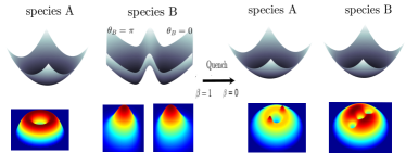
Figure 1: Schematic representation of the considered setup and the quench protocol. A vortex of unit charge is initially imprinted at the trap center of species A and a $\displaystyle\pi$ relative phase difference between the segments of species B. At $\displaystyle t=0$ we suddenly ramp down the potential barrier of species B, thus quenching its trapping geometry from a 2D spatially anisotropic harmonic trap to an isotropic one (see also Sec. II.1). This process leads to the generation of vortices in species B and density humps in species A.

For our purposes, after preparing the two BECs in a 2D harmonic potential, we use a repulsive barrier in the spirit of Scherer et al. (2007); Carretero-González et al. (2008b) to segregate species B into two isolated segments [see Fig. 1]. The potential barrier reads $\displaystyle V_{L}=\beta(t)U_{0}e^{-\frac{x^{2}}{2a^{2}}}$, with $\displaystyle U_{0}$ and $\displaystyle a$ being the height and the width parameters of the potential barrier respectively. Initially, $\displaystyle\beta(t)=1$ and depending on the functional form of $\displaystyle\beta(t)$ in $\displaystyle V_{L}$, various quench protocols of the barrier height can be realized. For instance, if $\displaystyle\beta(t)=1$ at $\displaystyle t<0$ and $\displaystyle\beta(t)=0$ for $\displaystyle t\geq 0$, this leads to a sudden quench [see Fig. 1], while e.g. $\displaystyle\beta(t)=(t_{f}-t)/t_{f}$ refers to a time-dependent removal of the barrier within a given ramp-down time $\displaystyle t_{f}$ which is not considered herein. Moreover, due to the the quasi-2D geometry i.e. $\displaystyle\omega_{z}\gg\omega_{x},\omega_{y}$ of the potential, the wavefunction of each species can be factorized as follows

$$\Psi_{\sigma}(x,y,z,t)=\psi_{\sigma}(x,y,t)\phi_{\sigma}(z).$$ (2)

Here, $\displaystyle\phi_{\sigma}(z)$ is the normalized ground state wavefunction in the $\displaystyle z$ direction. Then the dimensionless form of the coupled GP equations of Eq. (1) after integrating over $\displaystyle\phi_{\sigma}(z)$, since we address a 2D system, is the following Bandyopadhyay et al. (2017)

$$\begin{split}i\frac{\partial\psi_{A}(x,y,t)}{\partial t}=&\bigg{[}-\frac{1}{2}\nabla^{2}_{\perp}+V_{A}(x,y)\\ &+\sum_{j=A,B}\mathcal{U}_{Aj}|\psi_{j}(x,y,t)|^{2}\bigg{]}\psi_{A}(x,y,t)\end{split}$$ (3)

and

$$\begin{split}i\frac{\partial\psi_{B}(x,y,t)}{\partial t}=&\bigg{[}-\frac{m_{r}}{2}\nabla^{2}_{\perp}+V_{B}(x,y,t)+\\ &\sum_{j=A,B}\mathcal{U}_{Bj}|\psi_{j}(x,y,t)|^{2}\bigg{]}\psi_{B}(x,y,t).\end{split}$$ (4)

In these expressions, $\displaystyle\nabla_{\perp}^{2}=\partial^{2}_{x}+\partial^{2}_{y}$ is the kinetic energy term, while $\displaystyle V_{A}(x,y)=(x^{2}+y^{2})/2$ and $\displaystyle V_{B}(x,y,t)=(x^{2}+y^{2})/2m_{r}+V_{L}$ denote the external potential of each species with mass ratio $\displaystyle m_{r}=m_{A}/m_{B}$. Moreover, $\displaystyle\mathcal{U}_{AA}=2N_{A}\sqrt{2\pi\lambda}a_{AA}/a_{osc}$ and $\displaystyle\mathcal{U}_{BB}=2N_{B}m_{r}\sqrt{2\pi\lambda}a_{BB}/a_{osc}$ refer to the $\displaystyle A$ and $\displaystyle B$ species intraspecies interaction strengths respectively while the interspecies one corresponds to $\displaystyle\mathcal{U}_{AB}=\sqrt{2\pi\lambda}N_{A}(m_{A}+m_{B})a_{AB}/m_{B}a_{osc}$. Also, $\displaystyle N_{\sigma}$ with $\displaystyle\sigma=A,B$ denotes the particle number of each species which is taken to be $\displaystyle N_{A}=N_{B}=10^{4}$ throughout this work.

II.2 Ingredients of the numerical simulations

To study the dynamics of the binary bosonic system, we numerically solve Eqs. (3) and (4) using a split-time Crank-Nicolson method Muruganandam and Adhikari (2009); Vudragović et al. (2012) adapted for binary condensates. In particular we obtain the initial state of the system, considering $\displaystyle\beta(t)=1$ in Eq. (4), by propagating Eqs. (3) and (4) in imaginary time, until the solution converges to the desired state. This state refers to either a singly quantized vortex or the ground state of species A and a $\displaystyle\pi$ relative phase difference between the segments of species B. To introduce a vortex of charge $\displaystyle l$ at the center of the A species we apply the following transformation $\displaystyle\psi_{A}\rightarrow\psi^{\prime}_{A}\exp[il\tan^{-1}(\frac{y}{x})]$ to the corresponding initial guess wavefunction $\displaystyle\psi^{\prime}_{A}$. Indeed this transformation, as we shall see below, results in a topological phase defect in $\displaystyle\psi_{A}$ around which arg($\displaystyle\psi_{A}$) winds by $\displaystyle 2\pi l$. A similar topological phase imprinting method has been employed experimentally Leanhardt et al. (2002) and theoretically Bandyopadhyay et al. (2017); Kuopanportti et al. (2019). Simultaneously, we impose the phase condition for the B species such that $\displaystyle\theta_{B}=\pi$ for $\displaystyle x\leq 0$ and $\displaystyle\theta_{B}=0$ for $\displaystyle x>0$ at the initial guess wavefunction. We remark that imprinting the phase only at the initial guess wavefunctions is adequate here since the spatial overlap between the two species is vanishing for our setup due to the presence of the potential barrier in species B. However, for spatially overlapping components one needs to imprint the corresponding phase at each time-instant of the imaginary time propagation in order to maintain the imprinted phase structure. Furthermore, the normalization of the $\displaystyle\sigma$ species wavefunction is ensured by utilizing the transformation $\displaystyle\psi_{\sigma}\rightarrow\frac{1}{\norm{\psi}}\psi_{\sigma}$ at every time-instant of the imaginary time propagation until the energy of the desired configuration is reached with a precision $\displaystyle 10^{-8}$. With these solutions at hand as initial conditions, at $\displaystyle t=0$, we study their evolution in real time up to $\displaystyle 500$ ms utilizing Eqs. (3) and Eq. (4). The simulations are carried out in a square grid consisting of $\displaystyle 400\times 400$ grid points with a grid spacing $\displaystyle\Delta x=\Delta y=0.05$. The time step of integration $\displaystyle\Delta t$ is chosen to be $\displaystyle 10^{-4}$. In this way we ensure the numerical convergence of our simulations.

II.3 Observables

To monitor the quench induced dynamics of the binary BEC, we utilize various observables. In order to investigate the dynamical formation of the vortices, we employ as a spatially resolved measure the vorticity of the $\displaystyle\sigma$ species namely

$$\Omega_{\sigma}=\nabla\times J_{\sigma},$$ (5)

with $\displaystyle J_{\sigma}=\frac{i}{2m_{\sigma}}(\psi_{\sigma}^{*}\nabla\psi_{\sigma}-\psi_{\sigma}\nabla\psi_{\sigma}^{*})$ being the velocity probability current. The overall vorticity of the system can be quantified via the integrated vorticity Ruben et al. (2008)

$$\mathcal{Z}_{\sigma}=\int\absolutevalue{\Omega_{\sigma}}dxdy.$$ (6)

We remark that, while $\displaystyle\Omega_{\sigma}$ offers a spatially resolved measure of the vorticity of each bosonic cloud, $\displaystyle\mathcal{Z}_{\sigma}$ reveals the overall vortical content of the $\displaystyle\sigma$ species. To explore the angular momentum transfer between the different species we calculate the expectation value of the angular momentum of each species along the $\displaystyle z$ direction

$$L^{\sigma}_{z}=-i\int\psi^{*}_{\sigma}(x\frac{\partial}{\partial y}-y\frac{\partial}{\partial x})\psi_{\sigma}dxdy.$$ (7)

Moreover, the total energy of the system reads

$$\begin{split}E(\psi_{A},\psi_{B})=&\int\bigg{[}\frac{\absolutevalue{\nabla\psi_{A}}^{2}}{2}+V_{A}(x,y)\absolutevalue{\psi_{A}}^{2}\\ &+\frac{m_{r}\absolutevalue{\nabla\psi_{B}}^{2}}{2}+V_{B}(x,y)\absolutevalue{\psi_{B}}^{2}\\ &+\sum_{\sigma=A,B}\frac{\mathcal{U}_{\sigma\sigma^{\prime}}}{2}\absolutevalue{\psi_{\sigma^{\prime}}}^{2}\absolutevalue{\psi_{\sigma}}^{2}\bigg{]}.\end{split}$$ (8)

To gain a deeper understanding of the different parts of the energy during the quench induced dynamics, it is appropriate to express the condensate wavefunction according to the Madelung transformation Madelung (1927), namely $\displaystyle\psi_{\sigma}(x,y,t)=\sqrt{n_{\sigma}(x,y,t)}e^{il_{\sigma}\theta_{\sigma}(x,y,t)}$, where $\displaystyle n_{\sigma}(x,y,t)$ and $\displaystyle\theta_{\sigma}(x,y,t)$ denote the density and the phase of the $\displaystyle\sigma$ species respectively and $\displaystyle l_{\sigma}$ is the $\displaystyle\sigma$ species vortex charge. Furthermore, we define $\displaystyle\sqrt{n_{\sigma}}{\bf u_{\sigma}}$ as the superfluid velocity weighted by the square root of the density, with $\displaystyle\bf u_{\sigma}=\nabla\theta_{\sigma}$. As a consequence, the total energy functional of Eq. (2) can be decomposed as follows

$$E=\sum_{\sigma=A,B}\big{[}E^{\rm kin}_{\sigma}+E^{\rm q}_{\sigma}+E^{\rm tr}_{\sigma}+E^{\rm int}_{\sigma}\big{]}+E^{\rm mu}.$$ (9)

In this expression, $\displaystyle E^{\rm kin}_{A}=(1/2)\int\absolutevalue{\sqrt{n_{\sigma}}\bf u_{\sigma}}^{2}dxdy$ and $\displaystyle E^{\rm kin}_{B}=(m_{r}/2)\int\absolutevalue{\sqrt{n_{\sigma}}\bf u_{\sigma}}^{2}dxdy$ is the kinetic energy of the A and the B species respectively. Furthermore, $\displaystyle E^{\rm q}_{\sigma}=(1/2)\int(\nabla\sqrt{n_{\sigma}})^{2}\differential x\differential y$ denotes the quantum pressure energy, $\displaystyle E^{\rm tr}_{\sigma}=(1/2)\int n_{\sigma}V_{\sigma}(x,y,t)\differential x\differential y$ is the potential (trap) energy, $\displaystyle E^{\rm int}_{\sigma}=(1/2)\int\mathcal{U}_{\sigma\sigma}n_{\sigma}^{2}\differential x\differential y$ refers to the self-interaction energy and $\displaystyle E^{\rm mu}=\int\mathcal{U}_{AB}n_{A}n_{B}\differential x\differential y$ is the mutual interaction energy between the different species. We are particularly interested in the kinetic energy part since it captures the very essence of the dynamics at different time scales. Indeed, $\displaystyle E^{\rm kin}_{\sigma}$ can be further decomposed into a compressible $\displaystyle E^{\rm kin,c}_{\sigma}$ and an incompressible $\displaystyle E^{\rm kin,ic}_{\sigma}$ part, which are associated with the kinetic energy of the sound waves and the swirls, respectively Nore et al. (1997). This decomposition is performed as follows. The velocity vector, $\displaystyle\sqrt{n_{\sigma}}{\bf u_{\sigma}}$ can be written as a sum over a solenoidal part, $\displaystyle{\bf u^{ic}_{\sigma}}$, and an irrotational part, $\displaystyle{\bf u^{c}_{\sigma}}$, namely, $\displaystyle\sqrt{n_{\sigma}}{\bf u_{\sigma}}=\sqrt{n_{\sigma}}{\bf u^{c}_{\sigma}}+\sqrt{n_{\sigma}}{\bf u^{ic}_{\sigma}}$ such that $\displaystyle\divergence{\bf u^{ic}_{\sigma}}=0$ and $\displaystyle\curl{\bf u^{c}}=0$. We next define the scalar, $\displaystyle\Phi$, and vector, $\displaystyle A$, potential of the velocity field which satisfy the relations $\displaystyle\sqrt{n_{\sigma}}{\bf u^{ic}_{\sigma}}=\curl{{\bf A}}$ and $\displaystyle\sqrt{n_{\sigma}}{\bf u^{c}_{\sigma}}={\nabla}\Phi$ respectively. Taking the divergence of the last expression we obtain the Poisson equation for the scalar field, i.e. $\displaystyle\laplacian{\Phi}=\divergence{\sqrt{n_{\sigma}}{\bf u_{\sigma}}}$. From this equation we can numerically determine the scalar potential Benyam Mebrate (2015) and consequently the corresponding field components $\displaystyle{\bf u^{c}_{\sigma}}$ and $\displaystyle{\bf u^{ic}_{\sigma}}$. Hence, the compressible and incompressible parts of the species kinetic energy $\displaystyle A$ [$\displaystyle B$] species can be explicitly written as $\displaystyle E^{\rm kin,c}_{A}=1/2\int\absolutevalue{\sqrt{n_{A}}{\bf u^{c}_{A}}}^{2}dxdy$ [$\displaystyle E^{\rm kin,c}_{B}=(m_{r}/2)\int\absolutevalue{\sqrt{n_{B}}{\bf u^{c}_{B}}}^{2}dxdy$] and $\displaystyle E^{\rm kin,ic}_{A}=(1/2)\int\absolutevalue{\sqrt{n_{A}}{\bf u^{ic}_{A}}}^{2}dxdy$ [$\displaystyle E^{\rm kin,ic}_{B}=(m_{r}/2)\int\absolutevalue{\sqrt{n_{B}}{\bf u^{ic}_{B}}}^{2}dxdy$] respectively.

III Dynamics of a slightly mass imbalanced mixture

Let us focus here on the case of a small mass imbalance of the two species of the binary BEC, which in particular corresponds to the experimentally relevant mixture of ⁸⁷Rb-⁸⁵Rb atomic species Papp et al. (2008). Moreover, the harmonic oscillator potential possesses a frequency, $\displaystyle\omega_{A}=\omega_{B}=2\pi\times 30.83Hz$ and the typical anisotropy parameters $\displaystyle\alpha=1$ and $\displaystyle\lambda=40$ of the trapping which have been realized experimentally Görlitz et al. (2001). It is important to mention at this point that it might be difficult to achieve species selective potentials for a binary BEC composed of different hyperfine states of the same atomic species. Indeed, commonly the detuning responsible for optical trapping is much larger than the underlying hyperfine spltting. Such a difficulty has been rectified only very recently by employing the so-called “tune-out” approach Rubio-Abadal et al. (2018). However, mixtures consisting of two distinct atomic species can be routinely trapped in species selective potentials exploiting both the “tune-in” and the “tune-out” optical trapping methods, see for details of the schemes Ref. LeBlanc and Thywissen (2007). Hence, employing a slightly mass imbalanced mixture the advantage is two fold. First, it alleviates the possible experimental challenges to realize a species selective potential. Second, the dynamical behavior of the issystem similar to the exactly mass balanced scenario. We shall also discuss how a significant mass imbalance between the species alters the quench-induced dynamics in section V.

III.1 Singly quantized vortex in species A

We start the discussion of our numerical results by investigating the nonequilibrium dynamics of a 2D binary bosonic system when a vortex of unit charge is imprinted in species A and $\displaystyle\pi$ phase difference occurs between the segments of species B. Experimentally, a single BEC can be segmented into two slices by deforming a harmonic trap into a double-well potential utilizing a radiofrequency-induced Zobay and Garraway (2001); Jo et al. (2007) or an optical dipole potential Wang et al. (2005) along a certain spatial direction. Also, a well-defined relative phase difference between the two emergent slices of the condensate can be established using a single two photon coupling pulse Hall et al. (1998). A (quasi-one-dimensional) phase imprinting protocol along the lines of Becker et al. (2008) can have a similar effect. We consider the experimentally relevant intraspecies scattering lengths Egorov et al. (2013); Papp et al. (2008), $\displaystyle a_{AA}=100.4a_{0}$ and $\displaystyle a_{BB}=95.0a_{0}$, where $\displaystyle a_{0}$ denotes the Bohr radius. Also we assume an interspecies scattering length $\displaystyle a_{AB}=60a_{0}$ and therefore the two species are in the miscible regime since $\displaystyle a_{AB}^{2}<a_{AA}a_{BB}$ is fulfilled Ao and Chui (1998); Timmermans (1998) . After preparing the above-mentioned system in its initial state characterized by specific intra- and interspecies interactions, the dynamics is triggered by a sudden ramp down of the potential barrier of species B. The height and width of the optical potential barrier are chosen to be $\displaystyle U_{0}=20.0\omega_{x}$ and $\displaystyle a=1.0a_{\rm osc}$ respectively. This latter quench protocol allows the two initially separated segments of species B to collide and perform a counterflow dynamics. The postquench dynamics of the system can be categorized into three different time scales. Indeed, as we shall discuss below, at the very early stages of the dynamics quasi-1D nonlinear fringes known as dark stripes are formed. These dark stripes being subjected to the snake instability Verma et al. (2017) break into several VAV pairs. Subsequently, these VAV pairs propagate within the condensate, interact with each other and eventually only a single VB soliton persists in the long-time dynamics of the system. Below we analyze the dynamics within each of the aforementioned time intervals in detail.

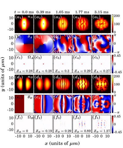
Figure 2: (Color online) Density profiles of ($\displaystyle a_{1}$)-($\displaystyle a_{5}$) species A and ($\displaystyle d_{1}$)-($\displaystyle d_{5}$) species B at various time instants (see legends) in the very early stages of the dynamics. The corresponding phase [vorticity] profiles of ($\displaystyle b_{1}$)-($\displaystyle b_{5}$) [($\displaystyle c_{1}$)-($\displaystyle c_{5}$)] species A and of ($\displaystyle e_{1}$)-($\displaystyle e_{5}$) [($\displaystyle f_{1}$)-($\displaystyle f_{5}$)] species B. The values of the $\displaystyle\sigma$ species integrated vorticity $\displaystyle\mathcal{Z}_{\sigma}$ are also shown within each vorticity profile. The binary BEC consisting of $\displaystyle N_{A}=N_{B}=10^{4}$ atoms is prepared in its ground state with a singly quantized vortex in species A and a $\displaystyle\pi$ phase difference in species B such that $\displaystyle\theta_{B}(x)=\pi$ for $\displaystyle x<0$ and $\displaystyle\theta_{B}(x)=0$ for $\displaystyle x\geq 0$. The intra- and interspecies scattering lengths are $\displaystyle a_{AA}=100.4a_{0}$, $\displaystyle a_{BB}=95a_{0}$ and $\displaystyle a_{AB}=60.0a_{0}$ respectively.

III.1.1 Density evolution

Figure 2 presents snapshots of the density, phase and vorticity profiles of both species at the early stages of the dynamics. We remark that due to the mutual interaction between the two species and the location of the potential barrier in species B, the initial density distribution of species A is elongated along the $\displaystyle y$-direction and in particular resides between the segments of species B [see Figs. 2 ($\displaystyle a_{1}$) and ($\displaystyle c_{1}$)]. As can be seen, the initial state of the system at $\displaystyle t=0$ ms, [Figs. 2 $\displaystyle(a_{1}),(b_{1}),(c_{1}),(d_{1}),(e_{1}),(f_{1})$], breaks into dark stripes in species B [Figs. 2 ($\displaystyle d_{2}$)-($\displaystyle d_{4}$), ($\displaystyle e_{2}$)-($\displaystyle e_{4}$) and ($\displaystyle f_{2}$)-($\displaystyle f_{4}$)] and bright stripes in species A [Figs. 2 ($\displaystyle a_{2}$)-($\displaystyle a_{4}$), ($\displaystyle b_{2}$)-($\displaystyle b_{4}$), ($\displaystyle c_{2}$)-($\displaystyle c_{4}$)] generated in the system directly after the merging of the two segments of species B. Subsequently, a disintegration of those stripes into vortices in species B [Figs. 2 $\displaystyle(d_{5}),(e_{5}),(f_{5})$] and localized density humps in species A [Figs. 2 $\displaystyle(a_{5})$] occurs.

In particular, directly after turning off the potential barrier the two segments of species B smoothly expand towards each other, while species A expands along the $\displaystyle x$- direction. The merged segments, initially possessing a $\displaystyle\pi$- relative phase difference, resemble an excited mode of the harmonic potential at $\displaystyle t>0$, see in particular a profile of the density in Fig. 2 ($\displaystyle d_{2}$) at $\displaystyle y=0$. As a result, a dark stripe of null density at the collision line accompanied by two lumps of higher atom density on its side are formed in species B [see Fig. 2 ($\displaystyle d_{2}$)]. At the same time, species A becomes more squeezed towards the collision line of species B leading to the formation of a bright stripe at the same place besides the trap center where the vortex is located [see Fig. 1 ($\displaystyle a_{2}$)]. Subsequently, the localized density dips (in species A) and humps (formed in species B) split into a larger number of dark and bright stripes respectively. For instance, as it can be noticed from the density profiles of species A (B) at $\displaystyle t=1.05$ ms, multiple bright (dark) stripes occur within the condensate density. Focusing on species B, we observe that, due to the non-uniform density of the condensate (due to the presence of the external trap and associated curvature), each dark soliton acquires a different velocity along the transverse $\displaystyle x$ direction. This leads to the bending of the soliton stripe and the resulting undulations lead to its eventual breakup into several VAV pairs Swartzlander et al. (1991); Toikka and Suominen (2013) as illustrated in Figs. 2 ($\displaystyle a_{3}$)-($\displaystyle a_{5}$) and ($\displaystyle d_{3}$)-($\displaystyle d_{5}$). Indeed, the formation of a chain of VAV pairs along the dark stripes, including a single vortex at the center of the middle stripe, can be noticed at $\displaystyle t=1.77$ ms and also even more pronouncedly at $\displaystyle t=3.15$ ms. Note that a decreasing amplitude of the dark solitons implies an increase of its transverse velocity Tikhonenko et al. (1996). Hence, due to the non-uniform density, the soliton stripes located close to the edge of the condensate bend faster than the ones residing in the middle [see also Figs. 2 ($\displaystyle d_{3}$) and ($\displaystyle d_{4}$)]. Moreover, as can be seen in Fig. 2 $\displaystyle(a_{3})$, dark stripes created in species B are filled by the atoms of species A, thus the density of species A localizes at the same place. This is natural as the former component acts as an effective potential for the latter one. Therefore, the generation of vortices in species B is accompanied by the formation of localized density humps (characterized by no phase jump across them) in species A resembling this way VB structures. We remark that such density peaks on the top of the BEC background are also known as antidark solitons Kivshar and Afanasjev (1991). Nevertheless, we will refer to these structures as VBs in what follows even when the bright component lies on top of a nontrivial background. Note that, bright solitons are bound states of the effective potential created by the vortices which stabilize the former. Otherwise, it would be impossible for the bright solitons to be sustained under the presence of repulsive interatomic interactions.

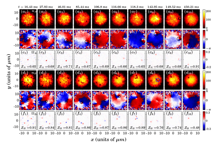
Figure 3: (Color online) Density profiles of ($\displaystyle a_{1}$)-($\displaystyle a_{10}$) species A and ($\displaystyle d_{1}$)-($\displaystyle d_{10}$) species B at various time instants (see legends) in the long-time evolution of the system. The corresponding phase [vorticity] profiles of ($\displaystyle b_{1}$)-($\displaystyle b_{10}$) [($\displaystyle c_{1}$)-($\displaystyle c_{10}$)] species A and of ($\displaystyle e_{1}$)-($\displaystyle e_{10})$ [($\displaystyle f_{1}$)-($\displaystyle f_{10}$)] species B. The value of the $\displaystyle\sigma$ species integrated vorticity at each depicted time instant is also provided within the corresponding vorticity profiles. The black circles in the phase profiles mark the location of vortices. The remaining system parameters are the same as in Fig. 2.

Having discussed the early stages of the dynamics, we next examine the longer time evolution of the system where a very rich dynamics of the generated VAV pairs takes place. Let us note in passing that the Gross-Pitaevskii equation has been extensively used to describe the long-time dynamics of similar setups Ruben et al. (2008); Tsatsos et al. (2016). Also, possible interparticle correlation effects are expected to be supressed due to the large particle number considered herein. The long-time dynamics is summarized in Fig. 3, which presents the density and vorticity profiles at selected time instants. After their production, the VAV pairs start to drift out of the condensate or they annihilate each other, see Fig. 2 ($\displaystyle d_{5}$) and Fig. 3 ($\displaystyle d_{1}$). The latter process reduces the number of vortices in species B. Indeed, inspecting Figs. 3 $\displaystyle(d_{1})$, ($\displaystyle e_{1}$) and $\displaystyle(f_{1})$, at $\displaystyle t=16.43$ ms, we observe that the VAV-V structure, which contains an antivortex at the center and two vortices placed on either side of the antivortex, is surrounded by several vortices [see Fig. 3 $\displaystyle(d_{1})$]. Gradually, these latter randomly spaced vortices around the VAV-V structure vanish, and only the VAV-V remains [see Fig. 3 $\displaystyle(d_{2})$ and $\displaystyle(f_{2})$] in species B. In the course of the dynamics, both vortices approach the antivortex several times and scatter [e.g. see Figs. 3 ($\displaystyle d_{2}$)-($\displaystyle d_{5}$) and ($\displaystyle f_{2}$)-($\displaystyle f_{5}$)]. After such a scattering event the VAV-V moves around the condensate keeping its linear arrangement intact [e.g. see Fig. 3 ($\displaystyle f_{2}$)-($\displaystyle f_{4}$)] or it precesses around the trap center where the linear arrangement of its constituents is distorted to a triangular one [Fig. 3($\displaystyle f_{3}$)-($\displaystyle f_{5}$)] Seman et al. (2010). Also, during the dynamics, one of the outermost vortices of the VAV-V reaches the surface of the cloud and excites surface modes. In turn, these surface modes can isolate the vortex (breaking in this way the VAV-V) at the edge of the cloud [see Fig. 3 $\displaystyle(d_{6})$ and $\displaystyle(d_{7})$]. At $\displaystyle t=142.95$ ms, as a result of the above breakup we observe that a structure is formed by the coalescence of the VAV pair near the edge of the cloud, see also the blue circle in Fig. 3 $\displaystyle(d_{8})$. Such a structure, is sometimes referred to as vortexonium Groszek et al. (2016), and it is hard to discern individual vortex phases although it remains a spatially localized bound state. More appropriately, this structure is known as the Jones-Roberts (JR) soliton (see, e.g., the recent discussion in Chiron and Scheid (2018)) and it has been recently considered also experimentally Meyer et al. (2017). As can be seen in Fig. 3 ($\displaystyle d_{9}$), the structure propagates towards the trap center and finally drifts out of the condensate leaving behind only a single vortex (from the original VAV-V structure).

On the other hand, the bright solitons generated in species A are located at the core of the vortices of species B. Recall that the existence of the bright solitons in species A is caused by the occurrence of vortices in species B. These bright solitons, being density humps on top of the BEC background of species A, certainly contribute to the inhomogeneity of the density of species A. Recall that a vortex experiences a density gradient from the condensate Bolda and Walls (1998); Jackson et al. (1999) which in turn creates a velocity field affecting its motion. If this density gradient is symmetrically distributed with respect to the position of the vortex, then the net velocity field acting on the vortex is zero and the vortex remains stationary in its original position. A close inspection of Figs. 3 ($\displaystyle a_{2}$)-($\displaystyle a_{3}$) reveals that the bright soliton structures building upon species A are not symmetrically distributed with respect to the trap center. Therefore, the vortex in species A experiences a net velocity field, towards the region of lower condensate density, which eventually displaces it from the trap center towards the periphery of the cloud. Subsequently, the displaced vortex precesses around the trap center Anderson et al. (2000), see Figs. 3 ($\displaystyle a_{4}$)-($\displaystyle a_{10}$), and persists in the long-time dynamics (see the discussion bellow).

III.1.2 Time evolution of the integrated vorticity

The dynamics of the system can further be understood by inspecting the time evolution of the integrated vorticity and of the different parts of the kinetic energy [see Eq. (9)] of the system. Recall that the integrated vorticity defined in Eq. (6) is a quantitative measure of the effects arising due to the vortical content of each species. In particular, if the $\displaystyle\sigma$ species does not (initially) contain any net vorticity, the area integral of $\displaystyle\Omega_{\sigma}$ without the modulus is zero owing to the cancellation between the regions of opposite vorticity. Clearly, this is not the case with the integrated vorticity, $\displaystyle\mathcal{Z}_{\sigma}$, which accounts for the overall vorticity present in the $\displaystyle\sigma$ species. As it can be seen from the inset of Fig. 4 $\displaystyle(a)$, the integrated vorticity of species A is initially non-zero, i.e. $\displaystyle\mathcal{Z}_{A}\neq 0$, due to the presence of the singly quantized vortex in species A. However, $\displaystyle\mathcal{Z}_{B}=0$, since at $\displaystyle t=0$ no vortex is present in species B. Moreover, the integrated vorticity of both species increases [Fig. 4 $\displaystyle(a)$] within the time interval $\displaystyle 0$ ms $\displaystyle<t<2$ ms since the collision of the segments of species B gives rise to a rapid generation of vortices and antivortices [e.g. see also Figs. 2 ($\displaystyle d_{3}$) and ($\displaystyle d_{5}$)]. Notice that this increase is associated with the absolute value in the definition of the relevant quantity, indicating that this diagnostic will increase even though there is no net vorticity gain within the dynamics. Then, $\displaystyle\mathcal{Z}_{B}$ decreases till $\displaystyle t=16$ ms, which suggests that the number of vortices in species B reduces, until the VAV-V structure is formed [see also Fig. 2 ($\displaystyle d_{5}$) and Fig. 3 ($\displaystyle d_{1}$)]. Within the time period between the formation of the VAV-V structure and the final single vortex stage, $\displaystyle\mathcal{Z}_{B}$ shows a highly fluctuating behavior around a mean value. On the other hand, $\displaystyle\mathcal{Z}_{A}$ increases upon the removal of the barrier but the overall vorticity of species B remains always larger than that of species A throughout the time evolution. After a single vortex finally persists in species B, $\displaystyle\mathcal{Z}_{A}$ and $\displaystyle\mathcal{Z}_{B}$ tend to approach each other.

III.1.3 Kinetic energy contributions

To shed further light onto the vortex dynamics of the system, we explore the time evolution of the different parts of the kinetic energy of each species. Note that, the incompressible kinetic energy, $\displaystyle E^{\rm kin,ic}_{\sigma}$, reveals the presence of vorticity in the $\displaystyle\sigma$ species, whereas the compressible kinetic energy, $\displaystyle E^{\rm kin,c}_{\sigma}$, is associated with the presence of acoustic waves. Let us first concentrate on the kinetic energy of species B. At $\displaystyle t=0$, there is no contribution to the energy from its kinetic part [see the right inset of Fig. 4 (b)]. However, shortly after the quench, $\displaystyle 0$ ms $\displaystyle<t<0.6$ ms, a rapid growth of $\displaystyle E^{\rm kin,c}_{B}$ is observed indicating the generation of acoustic waves. In fact, the undulations of the dark soliton stripes contribute to the acoustic waves that lead to the generation of vorticity in the system. For later evolution times, $\displaystyle 0.6$ ms $\displaystyle<t<2.0$ ms the generation of vortices causes the increasing behavior of $\displaystyle E^{\rm kin,ic}_{B}$, while $\displaystyle E^{\rm kin,c}_{B}$ decreases. Indeed, $\displaystyle E^{\rm kin,c}_{B}$ acquires a minimum value at $\displaystyle t=2$ ms, when $\displaystyle E^{\rm kin,ic}_{B}$ is maximized. This suggests that the generation of vortices into the system within this time interval might be attributed to the conversion of the acoustic energy into the swirling energy. Subsequently, as most of the vortices drift out of the condensate or annihilate each other, and in the process emit acoustic waves Leadbeater et al. (2001), a steep decrease of $\displaystyle E^{\rm kin,ic}_{B}$ accompanied by an increase of $\displaystyle E^{\rm kin,c}_{B}$ occurs until $\displaystyle t=16$ ms, where the above discussed VAV-V is formed [see also Fig. 4 (b)]. The VAV-V structure gradually converts its energy into acoustic energy within the time interval $\displaystyle 16$ ms $\displaystyle\leq t\leq 149$ ms, and then finally a pair of vortices is ejected into the background leaving behind a single vortex.

This final stage involving a single vortex can be noticed from the drop of $\displaystyle E^{\rm kin,ic}_{A}$ which afterwards remains almost stationary in time. By virtue of the initial vortex configuration, the kinetic energy of species A is dominated by its incompressible counterpart, $\displaystyle E^{\rm kin,ic}_{A}$. Although species A is confined in a rotationally symmetric harmonic trap, due to the interspecies interaction its density is compressed to the region where the potential barrier of species B is located, i.e., species B forms an effective potential which further confines species A. However, due to the interspecies interaction the merging process occurring in species B also affects the density of species A. In particular, as species A expands after the removal of the barrier, acoustic waves are also generated in species A, resulting in the rise of $\displaystyle E^{\rm kin,c}_{A}$ [see Fig.4 (e)]. Overall, $\displaystyle E^{\rm kin,ic}_{A}$ decreases while $\displaystyle E^{\rm kin,c}_{A}$ increases during the time evolution. Moreover, all components of the kinetic energy remain almost stationary for $\displaystyle t\geq 330$ ms, when the vortical patterns in each component have essentially settled. However, fluctuations around their mean values reveal the occurrence of energy exchange among the compressible and the incompressible parts of the velocity field. It is also worthwhile to note that $\displaystyle E^{\rm kin,ic}_{A}$, possessing initially the dominant contribution of the kinetic energy, for $\displaystyle t\geq 50$ ms becomes the smallest contributor to the total kinetic energy of the system. This raises the very important question on how vorticity of species A decays over time, and whether it is transferred to species B.

III.1.4 Dynamics of the angular momentum

To further unravel the dynamics of the vorticity of both species, we resort to the expectation value of the angular momentum of each species, $\displaystyle L^{\sigma}_{z}(t)$ [see also Eq. (7)] along the $\displaystyle z$- direction, as shown in Fig. 4 (c). Evidently, at $\displaystyle t=0$ ms the average angular momentum per particle of species A is unity, while for species B is zero, given their respective vorticities. Remarkably enough, the angular momentum of each species is not conserved after the removal of the barrier. A rapid angular momentum exchange between the two species takes place throughout the time evolution and a net angular momentum is gained by species B resulting eventually in $\displaystyle L^{A}_{z}\leq L^{B}_{z}$. Moreover, both species acquire a non integer angular momentum per particle. We remark here that the merging of the two segments in species B actually changes the rotational properties of the system by leading it to acquire vortices in the periphery of the cloud and thus to rotate in a nearly rigid-body rotation as a result White et al. (2016); A. and T (2017). It is also important to stress that the above-described angular momentum transfer among the different species depends on the initially imprinted relative phase difference between the segments of species B. For instance, herein, we found that a net angular momentum transfer is possible when a $\displaystyle\pi$ relative phase difference exists initially between the segments of species B. However, imprinting a zero phase difference between the segments, no such transfer process has been found (see also Appendix. B for a detailed investigation of the dependence of the angular momentum transfer on the above-mentioned phase difference is certainly of interest but lies beyond the scope of the present work.

To understand the above-described transfer of angular momentum between the species, we next derive the corresponding time evolution of the angular momentum of each species. Indeed it can be shown (see also Appendix B) that

$$\begin{split}\frac{\differential L^{A}_{z}}{\differential t}=&-\int\absolutevalue{\psi_{A}(x,y)}^{2}(x\frac{\partial}{\partial y}-y\frac{\partial}{\partial x})V_{A}(x,y)dxdy\\ &-\int\absolutevalue{\psi_{A}(x,y)}^{2}(x\frac{\partial}{\partial y}-y\frac{\partial}{\partial x})\mathcal{N}_{A}(x,y)dxdy\end{split}$$ (10)

and

$$\begin{split}\frac{\differential L^{B}_{z}}{\differential t}=&-\int\absolutevalue{\psi_{B}(x,y)}^{2}(x\frac{\partial}{\partial y}-y\frac{\partial}{\partial x})V_{B}(x,y)dxdy\\ &-\int\absolutevalue{\psi_{B}(x,y)}^{2}(x\frac{\partial}{\partial y}-y\frac{\partial}{\partial x})\mathcal{N}_{B}(x,y)dxdy.\end{split}$$ (11)

In these expressions, $\displaystyle V_{A}$ and $\displaystyle V_{B}$ denote the external trapping potentials of species A and species B respectively [see also Eqs. (3) and (4)]. Furthermore, $\displaystyle\mathcal{N}_{A}(x,y)$ = $\displaystyle\mathcal{U}_{AA}\absolutevalue{\psi_{A}(x,y)}^{2}+\mathcal{U}_{AB}\absolutevalue{\psi_{B}(x,y)}^{2}$ and $\displaystyle\mathcal{N}_{B}(x,y)=\mathcal{U}_{BB}\absolutevalue{\psi_{B}(x,y)}^{2}+\mathcal{U}_{AB}\absolutevalue{\psi_{A}(x,y)}^{2}$ are the corresponding nonlinear interaction energy terms. Most importantly, each of the Eqs. (10) and (11) can be divided into two parts. The first one includes the angular momentum operator and the external potential. This term vanishes for a spatially isotropic external potential and yields a non-zero contribution which becomes more significant for a larger spatial anisotropy. Since in our case we consider a sudden quench of the potential barrier then at $\displaystyle t>0$ the post-quench external potential is indeed isotropic and therefore this term vanishes. The second part of the Eqs. (10) and (11) captures the contribution from the nonlinear interaction term. In particular, it indicates that if the nonlinear interaction term is spatially isotropic then its contribution is zero but not if it is anisotropic. For our setup the densities of both species after the quench are anisotropic [see Figs. 2 ($\displaystyle a_{2}$) and ($\displaystyle d_{2}$)] and therefore this term is responsible for the observed angular momentum transfer. We have indeed verified the above-mentioned argumentation also within our simulations (results not shown here for brevity).

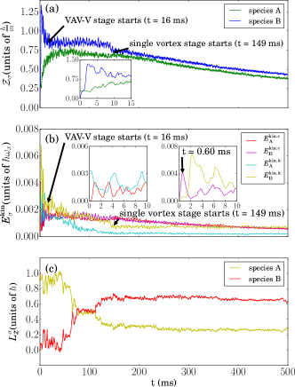
Figure 4: (Color online) (a) Time evolution of the integrated vorticity $\displaystyle\mathcal{Z}_{\sigma}(t)$ of each species. Inset shows $\displaystyle\mathcal{Z}_{\sigma}(t)$ within the time interval $\displaystyle 0$ ms $\displaystyle<t<10$ ms. (b) Compressible, $\displaystyle E^{\rm kin,c}_{\sigma}$, and incompressible, $\displaystyle E^{\rm kin,ic}_{\sigma}$, parts of the kinetic energy of the $\displaystyle\sigma$ species (see legend) during the evolution. Insets present $\displaystyle E^{\rm kin,c}_{A}$ and $\displaystyle E^{\rm kin,ic}_{A}$ (left panel) and $\displaystyle E^{\rm kin,c}_{B}$ and $\displaystyle E^{\rm kin,ic}_{B}$ (right panel) at the initial stages of the dynamics. The black arrows in (a), (b) indicate the time instants that the VAV stage and the singly quantized vortex stage start in species B. (c) Dynamics of the angular momentum, $\displaystyle L^{\sigma}_{z}(t)$, of the $\displaystyle\sigma=A,B$ species along the $\displaystyle z$ direction. The remaining system parameters are the same as in Fig. 2.

III.1.5 Effect of the interspecies interactions

After having explained the mechanism behind the angular momentum transfer we next discuss how this transfer is affected by the interspecies interaction strength. More specifically, we are interested in investigating how the degree of miscibility impacts the angular momentum transfer. Recall that homogeneous binary condensates are termed miscible when $\displaystyle a^{2}_{AB}\leq a_{AA}a_{BB}$ is fulfilled, and immiscible when $\displaystyle a^{2}_{AB}\geq a_{AA}a_{BB}$ holds Ao and Chui (1998); Timmermans (1998). However, under the presence of an external confinement this condition is modified due to the inhomogeneity of the density profiles Navarro et al. (2009); Wen et al. (2012); Bisset et al. (2018). A well-known measure of the degree of the phase separation, namely the degree of miscibility or immiscibility, is the overlap integral between the two species Mistakidis et al. (2018)

$$\Lambda=\frac{\biggr{[}\displaystyle\int\displaystyle\int{\rm d}x\hskip 1.42271pt{\rm d}y\hskip 1.42271ptn_{A}(x,y)\hskip 1.42271ptn_{B}(x,y)\biggr{]}^{2}}{\biggr{[}\displaystyle\int\displaystyle\int{\rm d}x\hskip 1.42271pt{\rm d}y\hskip 1.42271ptn_{A}^{2}(x,y)\biggr{]}\biggr{[}\displaystyle\int\displaystyle\int{\rm d}x\hskip 1.42271pt{\rm d}y\hskip 1.42271ptn_{B}^{2}(x,y)\biggr{]}}.$$ (12)

Here, $\displaystyle\Lambda(x,y,t)=0$ and $\displaystyle\Lambda(x,y,t)=1$ indicate zero (i.e., phase separation) and complete (i.e., phase mixing) spatial overlap between the two species, respectively.

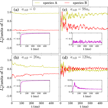
Figure 5: (Color online) Time evolution of the angular momentum, $\displaystyle L^{\sigma}_{z}(t)$, of the $\displaystyle\sigma$ species for (a) $\displaystyle a_{AB}=0$, (b) $\displaystyle a_{AB}=20a_{0}$, (c) $\displaystyle a_{AB}=98a_{0}$ and (d) $\displaystyle a_{AB}=120a_{0}$. The insets show the evolution of the corresponding overlap integral. The other system parameters are the same as in Fig. 3. The initial state of the mixture corresponds to an immiscible phase for all interspecies interactions due to the presence of the potential barrier in species B.

Figure 5 presents $\displaystyle L^{A}_{z}(t)$ [$\displaystyle L^{B}_{z}(t)$] of species A [species B] for various interspecies interaction strengths. $\displaystyle\Lambda(t)$ is also illustrated in the corresponding insets. Note that, due to the presence of the barrier, $\displaystyle\Lambda(t)$ is zero initially ($\displaystyle t=0$) for each interspecies interaction. For $\displaystyle a_{AB}=0$, $\displaystyle L^{A}_{z}(t)$ and $\displaystyle L^{B}_{z}(t)$ evolve independently keeping their initial angular momentum almost intact [see Fig. 5(a)]. This suggests that no angular momentum is transferred from species A to species B, while $\displaystyle\Lambda(t)\rightarrow 1$ rapidly [see the inset of Fig. 5 (a)]. However, as $\displaystyle a_{AB}$ is increased to $\displaystyle 20a_{0}$, a small portion of angular momentum is transferred to species B, yet the angular momentum of species A remains always higher than that of species B. The corresponding overlap integral $\displaystyle\Lambda(t)$ rapidly approaches unity indicating a miscible behavior between the species [see the inset of Fig. 5 (b)]. In contrast to the above a notable angular momentum transfer between the species occurs when a sufficiently large interspecies interaction is introduced. Indeed, for $\displaystyle a_{AB}=60a_{0}$, we observe that the angular momentum of species B exceeds that of species A [see Fig. 4 (c)]. This situation drastically changes at the border between the miscible to the immiscible regime, i.e., $\displaystyle a_{AB}=98a_{0}$. In this case species A transfers all of its angular momentum to species B just after the collision of the two segments. But shortly after the above-mentioned exchange species B transfers again its angular momentum back to species A, and both species feature an angular momentum exchange, until species A (approximately) acquires its initial angular momentum [see Fig. 5 (c)]. Here, $\displaystyle\Lambda(t)$ shows small fluctuations in time around 0.25 as illustrated in the inset of Fig. 5 (c). Entering the phase separated regime with $\displaystyle a_{AB}=120a_{0}$, the two species are initially spatially separated and they possess different angular momentum [see Fig. 5 (d)]. After the quench $\displaystyle t>0$ we observe an angular momentum transfer between the species and eventually at longer evolution times, $\displaystyle t>90$ ms, $\displaystyle L^{B}_{z}(t)$ becomes slightly larger than $\displaystyle L^{A}_{z}(t)$. This difference between $\displaystyle L^{A}_{z}(t)$ and $\displaystyle L^{B}_{z}(t)$ results in a nonzero overlap integral even in the immiscible regime [see the inset of Fig. 5 (d)]. Note here that the density of species A resides in between the segments of species B and therefore if $\displaystyle L^{A}_{z}(t)\neq L^{B}_{z}(t)$ the two species favor a spatial overlap between them. We remark that since $\displaystyle L^{A}_{z}(t)$ and $\displaystyle L^{B}_{z}(t)$ are finite in the long-time dynamics of the system, a single vortex builds upon each of the species and remains almost stationary for $\displaystyle t>100$ ms (results not shown for brevity).

IV Dynamics of a slighlty mass balanced mixure with zero vorticity in species A

Here we analyze the emergent nonequilibrium dynamics of the ⁸⁷Rb-⁸⁵Rb system when the initial configuration of species B contains a relative phase difference of $\displaystyle\pi$ between its segments, but species A possesses zero vorticity. Recall that species A is trapped in an isotropic 2D harmonic oscillator potential while species B is confined in an anisotropic trap consisting of a harmonic oscillator of equal frequencies in both directions and a potential barrier in the $\displaystyle y$ direction. With this configuration as initial state of our system, we again suddenly ramp down the barrier at $\displaystyle t=0$ ms, and let the system to evolve till $\displaystyle t=500$ ms. The density, phase and vorticity profiles of both species at various time instants are presented in Fig. 6. As in the previous section, we observe that after the quench the collision between the segments of species B generates dark and bright stripes in species B and species A respectively, see also Figs. 6 ($\displaystyle a_{2}$)-($\displaystyle d_{2}$). Subsequently, the dark and bright stripes break into VAV pairs [Fig. 6 ($\displaystyle d_{4}$)-($\displaystyle d_{5}$)] and bright solitons [Fig. 6 ($\displaystyle a_{4}$)-($\displaystyle a_{5}$)] respectively through the manifestation of the snake instability [see Fig. 6 ($\displaystyle d_{2}$)]. For long evolution times the aforementioned structures via their interactions eventually result in vortex-bright-soliton entities [Fig. 6 ($\displaystyle a_{5}$), ($\displaystyle d_{5}$)]. It is also important to note that the VAV pairs building upon species B, in the process of interacting and annihilating each other, produce two VAV dipoles. For instance, inspecting Figs. 6 ($\displaystyle d_{3}$), ($\displaystyle e_{3}$) and ($\displaystyle f_{3}$) we observe that one VAV pair resides at the trap center of the condensate, and another pair at the edges. However, this structure is not stable, since one vortex pair moves out of the condensate [see Fig. 6($\displaystyle d_{4}$), ($\displaystyle e_{4}$) and $\displaystyle(f_{4})$], resulting in a vortex dipole in species B and a pair of bright-solitons in species A.

The VAV pair formed close to the trap center creates an effective potential localizing bright-solitons of species A therein. We remark that a VAV pair with long lifetime has already been detected in numerous recent experiments Neely et al. (2010); Middelkamp et al. (2011); Kwon et al. (2015), where they are generated through a diverse set of experimental techniques (including dragging of a repulsive light barrier or quenching through the BEC transition). Recall that with the same initial phase configuration, species B produces a single vortex, when species A carries initially one unit vortex charge. Hence, given the relative $\displaystyle\pi$ phase difference between the segments of species B, it is the initial phase configuration of species A which plays a crucial role towards the generation of such topological defects (and especially so a net topological charge) in species B.

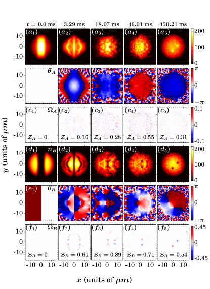
Figure 6: (Color online) Density profiles of ($\displaystyle a_{1}$)-($\displaystyle a_{5}$) species A and ($\displaystyle d_{1}$)-($\displaystyle d_{5}$) species B at selected time instants of the evolution. Shown are also the corresponding phase [vorticity] profiles of ($\displaystyle b_{1}$)-($\displaystyle b_{5}$) [($\displaystyle c_{1}$)-($\displaystyle c_{5}$)] species A and ($\displaystyle e_{1}$)-($\displaystyle e_{5}$) [($\displaystyle f_{1}$)-($\displaystyle f_{5}$)] species B. The value of the $\displaystyle\sigma$ species integrated vorticity is provided within the corresponding vorticity profiles. The binary BEC consists of $\displaystyle N_{A}=N_{B}=10^{4}$ bosons and it is prepared in its ground state with no vortex in species A and a phase difference in species B such that $\displaystyle\theta_{B}(x)=\pi$ for $\displaystyle x<0$ and $\displaystyle\theta_{B}(x)=0$ for $\displaystyle x\geq 0$. The intraspecies scattering lengths are $\displaystyle a_{AA}=100.4a_{0}$ and $\displaystyle a_{BB}=95a_{0}$, while the interspecies scattering length is $\displaystyle a_{AB}=60.0a_{0}$

.

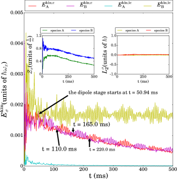
Figure 7: (Color online) Time evolution of the various parts of the kinetic energy (see legends). Inset shows the integrated vorticity (left panel) and the angular momentum (right panel) during the dynamics. The arrow indicates the time instant at which the dipole is created in species B. The remaining system parameters are the same as in Fig. 6

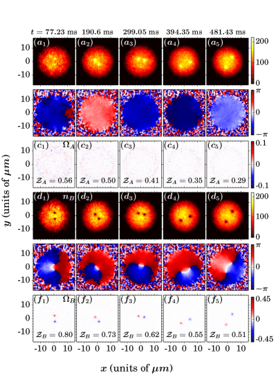
Figure 8: (Color online) Density profiles of ($\displaystyle a_{1}$)-($\displaystyle a_{5}$) species A and ($\displaystyle d_{1}$)-($\displaystyle d_{5}$) species B at long evolution times. The respective phase [vorticity] profiles of ($\displaystyle b_{1}$)-($\displaystyle b_{5}$) [($\displaystyle c_{1}$)-($\displaystyle c_{5}$)] species A and ($\displaystyle e_{1}$)-($\displaystyle e_{5}$) [($\displaystyle f_{1}$)-($\displaystyle f_{5}$)] species B are also presented in order to illustrate the dynamics of the vortex dipole. The integrated vorticity of each species at the depicted time instants is shown within the corresponding vorticity profiles. The remaining system parameters are the same as in Fig. 6

IV.0.1 Dynamics of the kinetic energy and the integrated vorticity

To further understand the dynamics we next investigate the behavior of the kinetic energy of the system as time evolves, see Fig. 7 $\displaystyle(a)$. Note that $\displaystyle E^{\rm kin,ic}_{A}$ is negligible throughout the time evolution, since there is no inherent or emergent vorticity present in species A. Indeed, the dynamics of species A is dominated by sound waves as it can be deduced by the finite value of $\displaystyle E^{\rm kin,c}_{A}$. However, as discussed in section III.1.2, $\displaystyle E^{\rm kin,ic}_{B}$ increases rapidly after the collision of the two segments signaling the generation of clusters of vortices. Also, one can indeed notice the annihilation of a large number of vortices and the production of a stable vortex structure from the time evolution of $\displaystyle E^{\rm kin,ic}_{B}$ and $\displaystyle E^{\rm kin,c}_{B}$. In particular, the decreasing behavior of $\displaystyle E^{\rm kin,ic}_{B}$ reveals that a large number of vortices annihilates until $\displaystyle t=50$ ms, contributing to an enhancement of the acoustic energy in the system. After the final, single vortex dipole remains, the $\displaystyle E^{\rm kin,ic}_{B}$ oscillates around a mean value with a periodically varying amplitude . This suggests that the motion of the dipole is affected by both the mutual interaction between the vortices and the spatial inhomogeneity of the condensate. Indeed, the vortex and the antivortex propel each other in their direction of flow Jones and Roberts (1982). It is also known Middelkamp et al. (2011, 2010) that for a VAV in a trap, the spatial inhomogeneity of the density drives each element of the pair to a direction which is opposite to their mutually driven motion. Depending on the competition between mutually driven motion and the spatial inhomogeneity, diverse trajectories might result, which essentially exhibit a quasi periodic behavior Middelkamp et al. (2011). Hence, the rapid oscillations of $\displaystyle E^{\rm kin,ic}_{B}$ in time stem from the aforementioned complicated quasi periodic motion of the vortex dipole Li et al. (2008). Figure 8 presents the density and vorticity profiles illustrating the dynamics of the vortex dipole. It becomes clear from Figs. 8 ($\displaystyle d_{1}$)-($\displaystyle d_{3}$) and ($\displaystyle f_{1}$)-($\displaystyle f_{3}$) that the dipole rotates around the trap center, and the distance between the vortex and antivortex fluctuates in time indicating their mutual interaction. The frequency of the rapid oscillation is determined by the mutual interaction between the pair, while the resulting envelope of the oscillation can be attributed to the precession of the pair around the trap center. Closely inspecting Fig. 7, it can be observed that whenever the amplitude of oscillation of $\displaystyle E^{\rm kin,ic}_{B}$ is small (large), a “chunk” of acoustic energy is emitted in species B (species A), see for example $\displaystyle E^{\rm kin,ic}_{B}$ at $\displaystyle 110$ ms $\displaystyle<t<165$ ms and $\displaystyle 165$ ms $\displaystyle<t<210$ ms and in particular the arrows in Fig. 7. A more detailed study on the dynamics of the vortex dipole can be found in Refs. Middelkamp et al. (2011, 2010).

The evolution of the integrated vorticity is also presented in the left inset of Fig. 7. At the early stages of the dynamics, $\displaystyle 0$ ms $\displaystyle<t<10$ ms, the integrated vorticity exhibits the same behavior as in section III.1.2. Namely, both $\displaystyle\mathcal{Z}_{A}$ and $\displaystyle\mathcal{Z}_{B}$ increase after the quench, reaching a maximum value and then show a decreasing behavior in time. However there are few noticeable differences. For instance, the maximum value of both the $\displaystyle\mathcal{Z}_{A}$ and the $\displaystyle\mathcal{Z}_{B}$ is smaller than their counterparts corresponding to the configuration with an initially singly quantized vortex imprinted in species A. Moreover, during the entire time evolution $\displaystyle\mathcal{Z}_{A}$ and $\displaystyle\mathcal{Z}_{B}$ remain quite disparate in their values. Indeed the overall vorticity of species A and species B is different since a vortex dipole is present in species B while no vortex is generated in species A. The behavior of the integrated vorticity of species A is dominated only by the acoustic waves, whereas that of species B is associated with both the vorticity and the acoustic waves. Finally, the angular momentum of both species remains close to its initial value throughout the evolution, see the right inset in Fig. 7.

For reasons of completeness let us also briefly comment on the effect when an initially zero phase difference between the segments of species B occurs and species A possesses zero vorticity (results not show here for brevity). Quenching the amplitude of the potential barrier of species B induces a counterflow dynamics of its segments and as a consequence dark and bright stripes form in species B and species A respectively. Then, the dark stripes formed in species B bend and two pairs of vortex dipoles are nucleated which evolve in time and subsequently one antivortex annihilates at the edge of the condensate resulting in the formation of a VAV-AV structure. As time evolves one of the participating antivortices of the VAV-AV structure moves out of the condensate resulting in a vortex dipole which undergoes a similar quasi periodic motion as discussed earlier in Sec. IV and eventually disappears. During the above-described dynamics of species B, the bright solitons formed in species A always accompany the vortex structures present in species B and of course reside at the same place. Moreover, the angular momentum of each of the species remains close to zero during the entire time evolution and therefore no transfer of angular momentum occurs.

V Dynamics of a strongly mass imbalanced mixture

Next we unravel the quench induced nonequilibrium dynamics of a binary condensate consisting of strongly imbalanced atomic species. Again, our focus is the initial configuration where species B contains a relative phase difference of $\displaystyle\pi$ between its segments and species A possesses a singly quantized vortex. Exemplarily, we consider the experimentally realizable mixture consisting of ⁸⁷Rb-¹³³Cs species where $\displaystyle m_{r}\approx 0.65$. In the following, for convenience, we label ⁸⁷Rb as species A and ¹³³Cs as species B. Moreover, the intraspecies scattering length of the ⁸⁷Rb and ¹³³Cs atoms correspond to $\displaystyle 100.4a_{0}$ and $\displaystyle 280a_{0}$ McCarron et al. (2011) respectively, whereas the interspecies scattering length is fixed to the value $\displaystyle 100a_{0}$. Furthermore, we use a harmonic oscillator potential of frequency, $\displaystyle\omega_{A}=\omega_{B}=2\pi\times 30.832Hz$ while the typical anisotropy parameters are taken to be $\displaystyle\alpha=1$ and $\displaystyle\lambda=40$ Görlitz et al. (2001). As in the previous section, after preparing the system in its initial state we suddenly ramp down the potential barrier in species B at $\displaystyle t=0$ and monitor the dynamics of the system.

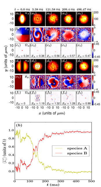
Figure 9: (Color online) Density profiles of ($\displaystyle a_{1}$)-($\displaystyle a_{5}$) species A (⁸⁷Rb) and ($\displaystyle d_{1}$)-($\displaystyle d_{5}$) species B (¹³³Cs) at selected time instants of the evolution. Also shown are the corresponding vorticity [phase] profiles of ($\displaystyle c_{1}$)-($\displaystyle c_{5}$) [($\displaystyle b_{1}$)-($\displaystyle b_{5}$)] species A and ($\displaystyle f_{1}$)-($\displaystyle f_{5}$)[($\displaystyle e_{1}$)-($\displaystyle e_{5}$)] species B. The integrated vorticity of each species at these time instants are shown in the corresponding profiles. The binary BEC consists of $\displaystyle N_{A}=N_{B}=10^{4}$ bosons and it is prepared in its ground state with a singly quantized vortex in species A and a phase difference in species B such that $\displaystyle\theta_{B}(x)=\pi$ for $\displaystyle x<0$ and $\displaystyle\theta_{B}(x)=0$ for $\displaystyle x\geq 0$. The intraspecies scattering lengths are $\displaystyle a_{AA}=100.4a_{0}$ and $\displaystyle a_{BB}=280.0a_{0}$, while the interspecies scattering length corresponds to $\displaystyle a_{AB}=100.0a_{0}$. (b) Dynamics of the angular momentum $\displaystyle L^{\sigma}_{z}(t)$ of the $\displaystyle\sigma=A,B$ species along the $\displaystyle z$ direction.

The emergent density and vorticity profiles of both species at different time-instants, following a quench of the potential barrier of species $\displaystyle B$, are presented in Fig. 9. A close inspection of the initial state [Figs. 9 ($\displaystyle a_{1}$), ($\displaystyle c_{1}$)] reveals that for the ⁸⁷Rb-¹³³Cs mixture the interface between the two species is flatter than that of the equal mass scenario [compare Fig. 9 ($\displaystyle c_{1}$) and Fig. 2 ($\displaystyle c_{1}$)]. This is due to the fact that while the presence of the potential barrier at the trap center prevents species B to occupy this spatial region, simultaneously the system desires to minimize its total energy by placing the heavier atoms close to the trap center. Directly after the barrier ramp down, the overall dynamics taking place is similar to the equal mass case, namely we observe the formation of V-AV pairs [Figs. 9 ($\displaystyle a_{3}$), ($\displaystyle b_{3}$), ($\displaystyle c_{3}$), ($\displaystyle d_{3}$)] via the snake instability, see Figs. 9 ($\displaystyle a_{2}$), ($\displaystyle c_{2}$) and Figs. 9 ($\displaystyle b_{2}$), ($\displaystyle d_{2}$) for the underlying phase profiles. Notice also that at the early stages of the dynamics [Figs. 9 ($\displaystyle c_{2}$)] a larger number of vortices is generated in species B which is composed of heavier atoms when compared to the almost mass balanced case [Fig 2($\displaystyle c_{5}$)]. Although these non-linear excitations interact and gradually decay they appear to be more robust [Fig. 9($\displaystyle c_{4}$)] compared to the equal mass scenario [Fig. 3($\displaystyle c_{7}$)] in the long-time dynamics of the system. This behavior is attributed to the fact that ¹³³Cs has a smaller healing length than ⁸⁵Rb since the former species is heavier and has a larger scattering length than the latter. Moreover, the vortices building upon species B and the corresponding bright solitons formed in species A during the dynamics exhibit a random motion in a very asymmetrical manner with respect to the trap center, see Figs. 9($\displaystyle c_{4}$) and ($\displaystyle c_{5}$). Phrased otherwise, the density humps (bright solitons) in species A are distributed non-uniformly with respect to the position of the initially imprinted vortex which in turn experiences a net velocity field created by the bright solitons. As a result, the initially imprinted vortex in species A is displaced from the trap center moving towards the edge of the condensate while performing a precessional motion [Fig. 9($\displaystyle c_{3}$)] and finally drifts out of the condensate [see Figs. 9($\displaystyle a_{3}$) and ($\displaystyle a_{4}$)]. Indeed, as shown in Fig. 9($\displaystyle c_{4}$) at $\displaystyle t=496.47$ ms there is a single V-AV pair located at the edge of the condensate and one vortex residing relatively close to the trap center. Concluding, the resultant spontaneously generated nonlinear structures appear to be more robust when species B possess a significantly larger mass than species A. Moreover, during the above-mentioned process, an ultimate transfer of angular momentum from species A to species B occurs, see Fig. 9($\displaystyle b$). Therefore we can deduce that even for the strongly mass imbalanced case the generic phenomenon of angular momentum transfer between the species takes place. Most importantly, for a strongly imbalanced mixture the angular momentum transfer is favored to a larger extent since the heavier species exhibits a smaller healing length and as a consequence it is possible to accommodate a larger amount of vortices. Indeed, as can be seen in Fig. 9($\displaystyle b$) the angular momentum of species B gradually reaches unity.

Finally, let us comment that for a lighter species B, for instance, assuming a ⁸⁷Rb-²³Na binary BEC Wang et al. (2015), due to the larger healing length of the ²³Na component, not only the number of the generated V-AV pairs decreases significantly, but they also decay rapidly during the dynamics (results not shown for brevity).

VI Conclusions

We have investigated the spontaneous generation of vortex-bright-solitons induced by merging two initially separated segments of one of the species in a two-dimensional binary BEC, considering both slight and considerable mass imbalance between the two species. The segmented species possess initially a $\displaystyle\pi$ phase difference between its segments while in the other species a singly quantized vortex or no vortex is imprinted. The merging of the segmented species is triggered by removing the potential barrier that initially separates the two segments of one of the species. We have described the outcome of the interference of the two initially separated segments and their effects on the other species. In particular, we have monitored the generation of vortex complexes, their motion and interactions within the clouds, and the resulting vortex-bright-soliton structure formation at long-time scales. The impact of the interspecies repulsion on the quench induced vortex generation and the dynamics of the angular momentum of both species have also been examined. To gain insights into the dynamics of the system, we have utilized several diagnostics such as the vorticity, the $\displaystyle z$ component of the angular momentum, the integrated vorticity and the compressible and incompressible parts of the kinetic energy.

In the first part of our study we considered a binary BEC with slightly mass imbalanced components. The initial configuration consists of a segmented species with a $\displaystyle\pi$ relative phase difference between the segments and a singly quantized vortex imprinted on the other species. A major finding here was the ultimate relaxation of species B into a state with a singly quantized vortex, caused by the angular momentum transfer from species A to species B. An accompanying bright soliton results in species A with the emerging vortex-bright (or,more precisely vortex-antidark) structure persisting for long times. In particular, after merging the two segments of species B we observe the generation of dark and bright soliton stripes in species B and species A respectively. These stripes break into VAV pairs Feder et al. (2000b) via the manifestation of the snake instability and subsequently form a VAV-V structure Seman et al. (2010) which evolves in the long-time dynamics into vortex-bright solitons. The overall dynamics can also be understood by inspecting the incompressible and compressible parts of the kinetic energy of the system being associated with the existence of vortices and sound waves respectively. Moreover, the transfer rate of the angular momentum between the species is found to crucially depend on the value of the interspecies interactions. More specifically for larger interspecies interactions, within the miscible regime of interactions, an increase of the transfer rate occurs while in the phase separated regime both species tend to share the same angular momentum.

As a next step, we consider an initial configuration in which a $\displaystyle\pi$ relative phase difference occurs between the segments of species B, but species A contains zero vorticity. As in the above-mentioned scenario the collision of the two segments of species B gives rise to dark and bright soliton stripes in both species which are subjected to the consequent modulational instability and break into vortex-antivortex pairs. In contrast to the previous case these vortex-antivortex pairs evolve into quadruples Yang et al. (2016) resulting in the long-time dynamics into a vortex dipole in species B accompanied by two bright solitons in species A. Another distinct feature of this configuration is the absence of angular momentum transfer between the species. Next, we inspected the effect of a heavier segmented species possessing also an experimentally relevant larger intraspecies scattering length. As a result the healing length of this heavier species becomes reduced compared to the mass balanced scenario and favors a complete transfer of angular momentum from species B to species A within the miscible regime of interactions. Moreover, the same overall phenomenology to the mass balanced case takes place during the dynamics while the quench-generated non-linear structures become more robust and persist in the long-time dynamics of the system. In other words, our computations suggest that the mass imbalance mainly affects the time scale of the appearance of the relevant phenomenology.

Summarizing, we can conclude that the robustness of the quench-induced topological structures and as a consequence the overall vortical activity of the binary condensate depends strongly on the mass imbalance between the two species. In particular, a slightly mass imbalanced mixture with a $\displaystyle\pi$ phase difference between the segments of species B and a singly quantized vortex imprinted in species A, leads ultimately to the persistence of a single vortex of unit charge in species B. However, with similar initial phases, increasing the mass of the species B to a fairly large value enhances the robustness of the quench-induced generated structures. In both cases, it should be noted that the structures are coupled to a bright (or more accurately anti-dark as it sits on top of a background Danaila et al. (2016); Kiehn et al. (2019)) soliton in the other species.

There are several interesting research directions to consider in future endeavors. A straightforward one is to examine the dynamical formation of vortex complexes when considering multiple fragments which possess an arbitrary relative phase difference between each other and unravel the corresponding quench dynamics upon ramping down the barriers that initially separate the fragments. Another interesting prospect would be to examine the dynamics of a harmonically trapped binary BEC where one of its components contains initially a multicharged vortex. Here, we have considered the case where the second species has a relative phase of $\displaystyle\pi$, however a more systematic study as a function of the relative phase of the two fragments in that species would be of interest in its own right. Moreover, the studies of the dynamics and interactions of these emerging vortex-bright (or vortex antidark) patterns that arise in these numerical experiments are equally interesting. Furthermore, this is the case both for the setting of same, as well as for that of opposite charge vortices. These investigations could also be extended to spin-orbit coupled BECs Stanescu et al. (2008); Wang et al. (2010); Lin et al. (2011) and dipolar BECs Góral and Santos (2002); Lahaye et al. (2009), where one can further inspect the impact of the additional interaction term among the particles on the vortex generation. The above-mentioned studies would also be equally interesting at the beyond mean-field Katsimiga et al. (2017a, b, 2018a, 2018b) level where intra- and interspecies correlations are taken into account.

Appendix A Dynamics of initially non-symmetric segments in the double-well

Here, we discuss the effect of an initial particle imbalance between the two segments of species B on the quench induced structure formation. As previously [Sec. III.1], species A is confined in an isotropic 2D harmonic oscillator and species B in an anisotropic trap composed of a harmonic oscillator of equal frequencies in both directions and a potential barrier in the $\displaystyle y$ direction. The intra- and interspecies scattering lengths correspond to $\displaystyle a_{AA}=100.4a_{0}$, $\displaystyle a_{BB}=95.0a_{0}$ and $\displaystyle a_{AB}=60a_{0}$ respectively. Also, the mixture is prepared such that the B species has a $\displaystyle\pi$ phase difference between its segments and species A contains a singly quantized vortex [Fig. 10($\displaystyle a_{1}$)]. However, in the present case we additionally impose a linear tilt of the form $\displaystyle-dx+c$ with $\displaystyle d=1$ and $\displaystyle c=10$ in the trap of the B species. This linear tilt essentially causes an energy offset between the left ($\displaystyle x<0$) and right ($\displaystyle x>0$) spatial regions of the B species potential resulting in a particle imbalance between the segments of species B. Consequently due to the particular choice of the parameters $\displaystyle d$, $\displaystyle c$ the left segment of species B possesses $\displaystyle 25\%N_{B}$ while the right segment has $\displaystyle 75\%N_{B}$ [Fig. 10 ($\displaystyle a_{2}$)]. As a result of the particle imbalance between the segments of species B and the finite positive value of $\displaystyle a_{AB}=60a_{0}$ also the density of species A exhibits initially an asymmetric configuration with respect to $\displaystyle x=0$ [Fig. 10 ($\displaystyle a_{1}$)]. In particular less particles of species A are located at $\displaystyle x>0$ since the atoms of species B are predominantly residing in this spatial direction ($\displaystyle x>0$) due to the presence of the tilt [Fig. 10 ($\displaystyle a_{1}$)] and subsequently repel the particles of species A to $\displaystyle x<0$. To induce the dynamics we then ramp down the potential barrier of species B and let the system to evolve. Monitoring the time-evolution of the $\displaystyle\sigma$ species angular momentum we observe that it is gradually transferred from species A to species B, see Fig. 10 ($\displaystyle a$). Closely inspecting $\displaystyle L^{\sigma}_{z}(t)$ we deduce that its transfer rate is maximized within the interval $\displaystyle 0<t<100$ ms. Most importantly, the angular momentun transfer between the species occurs faster for this particle-imbalanced case of species B as compared to the particle balanced scenario discussed in Sec. III.1 and presented in Fig. 5 ($\displaystyle c$). Another noticeable difference in the behavior of $\displaystyle L^{\sigma}_{z}(t)$ between the particle balanced [Fig. 5($\displaystyle c$)] and imbalanced [Fig. 10 ($\displaystyle c$)] case is that $\displaystyle L^{\sigma}_{z}$ exhibits a more pronounced oscillatory behavior in the latter case and also the mean value of $\displaystyle L^{A}_{z}(t)$ [$\displaystyle L^{B}_{z}(t)$] in the long-time dynamics is larger [smaller]. However, as in the particle balanced case, each of the species contains a single vortex in the long-time dynamics of the system, see e.g. Figs. 10($\displaystyle a_{3}$)-($\displaystyle a_{4}$). This clearly reveals that the non-linear structure formation in the long-time dynamics depends mainly on the phase difference between the segments of species B, while a particle imbalance between these segments only alters the time scale of the manifestation of the relevant phenomenology.

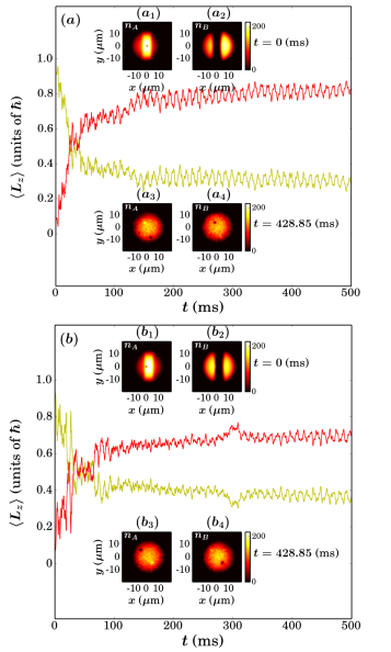
Figure 10: ($\displaystyle a$) Temporal evolution of the $\displaystyle\sigma=A,B$ species angular momentum $\displaystyle L^{\sigma}_{z}(t)$ along the $\displaystyle z$ direction when there is an initial particle imbalance between two segments. Snapshots of the $\displaystyle\sigma$ species density (see legends) at ($\displaystyle a_{1}$)-($\displaystyle a_{2}$) the initial time ($\displaystyle t=0$ ms) and ($\displaystyle a_{3}$)-($\displaystyle a_{4}$) the long-time ($\displaystyle t=428.85$ ms) dynamics of the system. ($\displaystyle b$) Dynamics of the angular momentum $\displaystyle L^{\sigma}_{z}(t)$ along the $\displaystyle z$ direction when the two segments of species B are not symmetrically located with respect to the trap center. Density snapshots of the $\displaystyle\sigma$ species at ($\displaystyle b_{1}$)-($\displaystyle b_{2}$) the initial time ($\displaystyle t=0$ ms) and ($\displaystyle b_{3}$)-($\displaystyle b_{4}$) the long-time dynamics ($\displaystyle t=428.85$ ms).

Next, we comment on the impact of another type of initial state imperfection on the quench dynamics of the mixture. Here, the initial state preparation is the same as in Sec. III.1 but the two segments of species B are not symmetrically placed with respect to the trap center $\displaystyle x=0$, see Fig. 10 ($\displaystyle b_{2}$). This can be achieved by considering a displaced potential barrier namely $\displaystyle V_{L}=\beta(t)U_{0}e^{-\frac{(x-x_{0})^{2}}{2a^{2}}}$, where $\displaystyle x_{0}=1a_{\rm osc}=1.94\mu m$, $\displaystyle\beta(t=0)=1$, $\displaystyle U_{0}=20\omega_{x}$ and $\displaystyle a=1a_{osc}$. As it can be seen, the vortex in species A is located at the trap center [Fig. 10($\displaystyle b_{1}$)] while the overall density of species A is somewhat shifted to $\displaystyle x>0$ due to the location of the potential barrier in species B at $\displaystyle x_{0}$. The dynamics of the $\displaystyle\sigma$ species angular momentum is illustrated in Fig. 10 ($\displaystyle b$) following a quench of the potential barrier height to zero. Evidently, an angular momentum transfer between the species occurs with a maximum transfer rate taking place within the interval $\displaystyle 0<t<100$ ms. Interestingly, the final value of $\displaystyle L^{\sigma}_{z}$ is very close to the one corresponding to the symmetrically located segments, compare Fig. 10($\displaystyle b$) and Fig. 5($\displaystyle c$). Moreover, we can infer that this initial state imperfection again modifies the time scales of the dynamical response of the mixture. This alteration of time scales can be directly observed in the dynamics of $\displaystyle L^{\sigma}_{z}$ between the case of $\displaystyle x_{0}=0$ [Fig. 5 ($\displaystyle c$)] and $\displaystyle x_{0}=1a_{\rm osc}$ [Fig. 10 ($\displaystyle b$)] However, in the long-time dynamics of the system only a single vortex persists in both species, see Figs. 10 ($\displaystyle b_{3}$), ($\displaystyle b_{4}$). Concluding, also this initial state imperfection does not alter both the non-linear structure formation in the long-time dynamics and the underlying transfer of angular momentum between the species.

Appendix B Derivation of the equations of evolution of the angular momentum

In this Appendix we provide the derivation of the equations of temporal evolution of the angular momentum of each species [see Eqs. (10) and (11)] used in the main text to explain the angular momentum transfer between the species during the nonequilibrium dynamics of the binary BEC. By invoking its definition [see Eq. (7)], the $\displaystyle z$ component of the angular momentum of the $\displaystyle\sigma$ species reads

$$L^{\sigma}_{z}=-i\int\differential S\psi^{*}_{\sigma}(x\partial_{y}-y\partial_{x})\psi_{\sigma},$$ (13)

where $\displaystyle\differential S=\differential x\differential y$ denotes the spatial area of integration. In our case it corresponds to the $\displaystyle x$-$\displaystyle y$ plane restricted by the hard-wall boundaries used herein, i.e. $\displaystyle x_{\pm}=y_{\pm}=\pm 10$. To proceed, we introduce the abbreviation $\displaystyle\tilde{L}=x\partial_{y}-y\partial_{x}$. Then we can express the angular momentum operator as $\displaystyle L_{z}=-i\tilde{L}$. Since $\displaystyle L_{z}$ is a self-adjoint operator we obtain also that $\displaystyle\tilde{L}^{\dagger}=-\tilde{L}$. Calculating the time-derivative of Eq. (13) and also using the above-mentioned abbreviation we arrive at the relation

$$\begin{split}\frac{\differential L^{\sigma}_{z}}{dt}=&-i\int\differential S\frac{\partial\psi^{*}_{\sigma}}{\partial t}\tilde{L}\psi_{\sigma}-i\int\differential S\psi_{\sigma}\tilde{L}\frac{\partial\psi^{*}_{\sigma}}{\partial t}\\ &=-i\int\differential S\frac{\partial\psi^{*}_{\sigma}}{\partial t}\tilde{L}\psi_{\sigma}+i\int\differential S\frac{\partial\psi}{\partial t}\tilde{L}\psi^{*}_{\sigma}.\end{split}$$ (14)

Subsequently, we replace the time-derivative of the $\displaystyle\sigma$ species wavefunction using the coupled set of GP equations [Eqs. (3) and (4) in the main text]. The resulting time-derivative of the angular momentum [Eq. (14)] reads

$$\begin{split}\frac{dL^{\sigma}_{z}}{dt}&=\int dS(-\frac{1}{2}\nabla^{2}_{\perp}\psi^{*}_{\sigma}+V_{\sigma}\psi^{*}_{\sigma}+\mathcal{N}_{\sigma}\psi^{*}_{\sigma})\tilde{L}\psi_{\sigma}\\ &+\int dS\tilde{L}\psi^{*}_{\sigma}(-\frac{1}{2}\nabla^{2}_{\perp}\psi_{\sigma}+V_{\sigma}\psi_{\sigma}+\mathcal{N}_{\sigma}\psi_{\sigma})\end{split}$$ (15)

Furthermore by substituting $\displaystyle L_{z}=-i\tilde{L}$ into the last equation and performing some algebra we obtain the following equation of motion of the $\displaystyle\sigma$ species angular momentum

$$\begin{split}&\frac{dL^{\sigma}_{z}}{dt}\\ &=\frac{1}{2}\int dS\big{[}\nabla^{2}_{\perp}\psi^{*}_{\sigma}(x\frac{\partial}{\partial y}-y\frac{\partial}{\partial x})\psi_{\sigma}+\nabla^{2}_{\perp}\psi_{\sigma}(x\frac{\partial}{\partial y}-y\frac{\partial}{\partial x})\psi^{*}_{\sigma}\big{]}\\ &+\int dS\big{[}V_{\sigma}\psi^{*}_{\sigma}(x\frac{\partial}{\partial y}-y\frac{\partial}{\partial x})\psi_{\sigma}dS+V_{\sigma}\psi^{*}_{\sigma}(x\frac{\partial}{\partial y}-y\frac{\partial}{\partial x})\psi_{\sigma}]\\ &+\int dS\big{[}\mathcal{N}_{\sigma}\psi^{*}_{\sigma}(x\frac{\partial}{\partial y}-y\frac{\partial}{\partial x})\psi_{\sigma}dS+\mathcal{N}_{\sigma}\psi^{*}_{\sigma}(x\frac{\partial}{\partial y}-y\frac{\partial}{\partial x})\psi_{i}].\end{split}$$ (16)

Here, $\displaystyle\mathcal{N}_{\sigma}=\sum_{\sigma^{\prime}}\mathcal{U}_{\sigma\sigma^{\prime}}\absolutevalue{\psi_{\sigma}}^{2}$ denotes the nonlinear interaction term. As it can readily seen by inspecting Eq. (16) there three different contributing terms, corresponding to the three different lines in Eq. (16), in the equation of motion of the angular momentum. It can be shown through a tedious but straightforward calculation that the first term associated with the kinetic energy of the system vanishes. The second and third terms related to the potential energy and the nonlinear interactions respectively reduce to expressions $\displaystyle-\int\differential S\absolutevalue{\psi_{\sigma}}^{2}(x\frac{\partial}{\partial y}-y\frac{\partial}{\partial x})V_{\sigma}$ and $\displaystyle-\int\differential S\absolutevalue{\psi_{\sigma}}^{2}(x\frac{\partial}{\partial y}-y\frac{\partial}{\partial x})\mathcal{N}_{\sigma}$. As a consequence the equation of motion of the angular momentum of the $\displaystyle\sigma$ species reads

$$\begin{split}\frac{dL^{\sigma}_{z}}{dt}=&-\int dS\absolutevalue{\psi_{\sigma}}^{2}(x\frac{\partial}{\partial y}-y\frac{\partial}{\partial x})V_{\sigma}\\ &-\int dS\absolutevalue{\psi_{\sigma}}^{2}(x\frac{\partial}{\partial y}-y\frac{\partial}{\partial x})\mathcal{N}_{\sigma}.\end{split}$$ (17)

These correspond exactly to the Eqs. (10) and (11) presented in the main text.

References

- Anderson et al. (1995) M. H. Anderson, J. R. Ensher, M. R. Matthews, C. E. Wieman, and E. A. Cornell, Science 269, 198 (1995).
- Davis et al. (1995) K. B. Davis, M. O. Mewes, M. R. Andrews, N. J. van Druten, D. S. Durfee, D. M. Kurn, and W. Ketterle, Phys. Rev. Lett. 75, 3969 (1995).
- Marzlin et al. (1997) K.-P. Marzlin, W. Zhang, and E. M. Wright, Phys. Rev. Lett. 79, 4728 (1997).
- Dalfovo and Stringari (1996) F. Dalfovo and S. Stringari, Phys. Rev. A 53, 2477 (1996).
- Rokhsar (1997) D. S. Rokhsar, Phys. Rev. Lett. 79, 2164 (1997).
- Dodd et al. (1997) R. J. Dodd, K. Burnett, M. Edwards, and C. W. Clark, Phys. Rev. A 56, 587 (1997).
- Jackson et al. (1998) B. Jackson, J. F. McCann, and C. S. Adams, Phys. Rev. Lett. 80, 3903 (1998).
- Fetter and Svidzinsky (2001) A. L. Fetter and A. A. Svidzinsky, Journal of Physics: Condensed Matter 13, R135 (2001).
- Kevrekidis et al. (2004a) P. Kevrekidis, R. Carretero-González, D. Frantzeskakis, and I. Kevrekidis, Mod. Phys. Lett. B 18, 1481 (2004a).
- Dennis et al. (2009) M. R. Dennis, K. O’Holleran, and M. J. Padgett, Prog. Optics 53, 293 (2009).
- Lugt (1983) H. J. Lugt, New York, Wiley-Interscience, 1983, 305 p. Translation. (1983).
- Libeskind et al. (2013) N. I. Libeskind, Y. Hoffman, M. Steinmetz, S. Gottlöber, A. Knebe, and S. Hess, The Astrophysical Journal 766, L15 (2013).
- Blatter et al. (1994) G. Blatter, M. V. Feigel’man, V. B. Geshkenbein, A. I. Larkin, and V. M. Vinokur, Rev. Mod. Phys. 66, 1125 (1994).
- Pismen (1999) L. M. Pismen, Oxford University Press, Oxford (1999).
- Onofrio et al. (2000) R. Onofrio, C. Raman, J. Abo-Shaeer, A. Chikkatur, and W. Ketterle, Phys. Rev. Lett. 85, 2228 (2000).
- Paoletti et al. (2008) M. S. Paoletti, M. E. Fisher, K. R. Sreenivasan, and D. P. Lathrop, Phys. Rev. Lett. 101, 154501 (2008).
- White et al. (2010) A. C. White, C. F. Barenghi, N. P. Proukakis, A. J. Youd, and D. H. Wacks, Phys. Rev. Lett. 104, 075301 (2010).
- Neely et al. (2013) T. W. Neely, A. S. Bradley, E. C. Samson, S. J. Rooney, E. M. Wright, K. J. H. Law, R. Carretero-González, P. G. Kevrekidis, M. J. Davis, and B. P. Anderson, Phys. Rev. Lett. 111, 235301 (2013).
- Kwon et al. (2014) W. J. Kwon, G. Moon, J.-y. Choi, S. W. Seo, and Y.-i. Shin, Phys. Rev. A 90, 063627 (2014).
- Matthews et al. (1999) M. R. Matthews, B. P. Anderson, P. C. Haljan, D. S. Hall, C. E. Wieman, and E. A. Cornell, Phys. Rev. Lett. 83, 2498 (1999).
- Anderson et al. (2000) B. P. Anderson, P. C. Haljan, C. E. Wieman, and E. A. Cornell, Phys. Rev. Lett. 85, 2857 (2000).
- Feder and Clark (2001) D. L. Feder and C. W. Clark, Phys. Rev. Lett. 87, 190401 (2001).
- Cooper et al. (2004) N. R. Cooper, S. Komineas, and N. Read, Phys. Rev. A 70, 033604 (2004).
- Isoshima and Machida (1999) T. Isoshima and K. Machida, Phys. Rev. A 59, 2203 (1999).
- Chevy and Stringari (2003) F. Chevy and S. Stringari, Phys. Rev. A 68, 053601 (2003).
- Coddington et al. (2003) I. Coddington, P. Engels, V. Schweikhard, and E. A. Cornell, Phys. Rev. Lett. 91, 100402 (2003).
- Baym (2003) G. Baym, Phys. Rev. Lett. 91, 110402 (2003).
- Mizushima et al. (2004) T. Mizushima, Y. Kawaguchi, K. Machida, T. Ohmi, T. Isoshima, and M. M. Salomaa, Phys. Rev. Lett. 92, 060407 (2004).
- Freilich et al. (2010) D. V. Freilich, D. M. Bianchi, A. M. Kaufman, T. K. Langin, and D. S. Hall, Science 329, 1182 (2010).
- Anderson (2010) B. P. Anderson, J. Low Temp. Phys. 161, 574 (2010).
- Navarro et al. (2013) R. Navarro, R. Carretero-González, P. J. Torres, P. G. Kevrekidis, D. J. Frantzeskakis, M. W. Ray, E. Altuntaş, and D. S. Hall, Phys. Rev. Lett. 110, 225301 (2013).
- Madison et al. (2000) K. W. Madison, F. Chevy, W. Wohlleben, and J. Dalibard, Phys. Rev. Lett. 84, 806 (2000).
- Middelkamp et al. (2011) S. Middelkamp, P. J. Torres, P. G. Kevrekidis, D. J. Frantzeskakis, R. Carretero-González, P. Schmelcher, D. V. Freilich, and D. S. Hall, Phys. Rev. A 84, 011605 (2011).
- Samson et al. (2016) E. C. Samson, K. E. Wilson, Z. L. Newman, and B. P. Anderson, Phys. Rev. A 93, 023603 (2016).
- Shibayama et al. (2011) H. Shibayama, Y. Yasaku, and T. Kuwamoto, J. Phys. B: At. Mol. Opt. Phys. 44, 075302 (2011).
- Räbinä et al. (2018) J. Räbinä, P. Kuopanportti, M. I. Kivioja, M. Möttönen, and T. Rossi, Phys. Rev. A 98, 023624 (2018).
- Leanhardt et al. (2002) A. E. Leanhardt, A. Görlitz, A. P. Chikkatur, D. Kielpinski, Y. Shin, D. E. Pritchard, and W. Ketterle, Phys. Rev. Lett. 89, 190403 (2002).
- Kumakura et al. (2006) M. Kumakura, T. Hirotani, M. Okano, T. Yabuzaki, and Y. Takahashi, Laser Phys. 16, 371 (2006).
- Shin et al. (2004) Y. Shin, M. Saba, M. Vengalattore, T. A. Pasquini, C. Sanner, A. E. Leanhardt, M. Prentiss, D. E. Pritchard, and W. Ketterle, Phys. Rev. Lett. 93, 160406 (2004).
- Mateo and Delgado (2006) A. M. Mateo and V. Delgado, Phys. Rev. Lett. 97, 180409 (2006).
- Andersen et al. (2006) M. F. Andersen, C. Ryu, P. Cladé, V. Natarajan, A. Vaziri, K. Helmerson, and W. D. Phillips, Phys. Rev. Lett. 97, 170406 (2006).
- Wright et al. (2008) K. C. Wright, L. S. Leslie, and N. P. Bigelow, Phys. Rev. A 77, 041601 (2008).
- Wright et al. (2009) K. C. Wright, L. S. Leslie, A. Hansen, and N. P. Bigelow, Phys. Rev. Lett. 102, 030405 (2009).
- Hodby et al. (2001) E. Hodby, G. Hechenblaikner, S. A. Hopkins, O. M. Maragò, and C. J. Foot, Phys. Rev. Lett. 88, 010405 (2001).
- Williams et al. (2010) R. A. Williams, S. Al-Assam, and C. J. Foot, Phys. Rev. Lett. 104, 050404 (2010).
- Hodby et al. (2003) E. Hodby, S. A. Hopkins, G. Hechenblaikner, N. L. Smith, and C. J. Foot, Phys. Rev. Lett. 91, 090403 (2003).
- Murray et al. (2009) D. R. Murray, P. Öhberg, D. Gomila, and S. M. Barnett, Phys. Rev. A 79, 063618 (2009).
- Zhao and Gu (2015) Q. Zhao and Q. Gu, Frontiers of Physics 10, 100306 (2015).
- Price et al. (2016) R. M. Price, D. Trypogeorgos, D. L. Campbell, A. Putra, A. Valdés-Curiel, and I. B. Spielman, New J. Phys. 18, 113009 (2016).
- Anderson et al. (2001) B. P. Anderson, P. C. Haljan, C. A. Regal, D. L. Feder, L. A. Collins, C. W. Clark, and E. A. Cornell, Phys. Rev. Lett. 86, 2926 (2001).
- Anglin and Zurek (1999) J. R. Anglin and W. H. Zurek, Phys. Rev. Lett. 83, 1707 (1999).
- Weiler et al. (2008) C. N. Weiler, T. W. Neely, A. S. Scherer, D. R. Bradley, M. J. Davis, and B. P. Anderson, Nature 455, 948 (2008).
- Andrews et al. (1997) M. R. Andrews, C. G. Townsend, H.-J. Miesner, D. S. Durfee, D. M. Kurn, and W. Ketterle, Science 275, 637 (1997).
- Myatt et al. (1997) C. J. Myatt, E. A. Burt, R. W. Ghrist, E. A. Cornell, and C. E. Wieman, Phys. Rev. Lett. 78, 586 (1997).
- Pitaevskii and Stringari (1999) L. Pitaevskii and S. Stringari, Phys. Rev. Lett. 83, 4237 (1999).
- Liu et al. (2000) W.-M. Liu, B. Wu, and Q. Niu, Phys. Rev. Lett. 84, 2294 (2000).
- Hadzibabic et al. (2004) Z. Hadzibabic, S. Stock, B. Battelier, V. Bretin, and J. Dalibard, Phys. Rev. Lett. 93, 180403 (2004).
- Kibble (1976) T. W. B. Kibble, J. Phys. A. Math. Gen. 9, 1387 (1976).
- Zurek (2009) W. H. Zurek, Phys. Rev. Lett. 102, 105702 (2009).
- Scherer et al. (2007) D. R. Scherer, C. N. Weiler, T. W. Neely, and B. P. Anderson, Phys. Rev. Lett. 98, 110402 (2007).
- Wallis et al. (1997) H. Wallis, A. Röhrl, M. Naraschewski, and A. Schenzle, Phys. Rev. A 55, 2109 (1997).
- Carretero-González et al. (2008a) R. Carretero-González, B. P. Anderson, P. G. Kevrekidis, D. J. Frantzeskakis, and C. N. Weiler, Phys. Rev. A 77, 033625 (2008a).
- Scott et al. (1998) T. F. Scott, R. J. Ballagh, and K. Burnett, J. Phys. B:At. Mol. Opt. Phys. 31, L329 (1998).
- Xiong et al. (2013) B. Xiong, T. Yang, and K. A. Benedict, Phys. Rev. A 88, 043602 (2013).
- Yang et al. (2013) T. Yang, B. Xiong, and K. A. Benedict, Phys. Rev. A 87, 023603 (2013).
- Mueller and Ho (2002) E. J. Mueller and T.-L. Ho, Phys. Rev. Lett. 88, 180403 (2002).
- Schweikhard et al. (2004) V. Schweikhard, I. Coddington, P. Engels, S. Tung, and E. A. Cornell, Phys. Rev. Lett. 93, 210403 (2004).
- Kuopanportti et al. (2012) P. Kuopanportti, J. A. M. Huhtamäki, and M. Möttönen, Phys. Rev. A 85, 043613 (2012).
- Kasamatsu and Tsubota (2009) K. Kasamatsu and M. Tsubota, Phys. Rev. A 79, 023606 (2009).
- Miesner et al. (1999) H.-J. Miesner, D. M. Stamper-Kurn, J. Stenger, S. Inouye, A. P. Chikkatur, and W. Ketterle, Phys. Rev. Lett. 82, 2228 (1999).
- Mertes et al. (2007) K. M. Mertes, J. W. Merrill, R. Carretero-González, D. J. Frantzeskakis, P. G. Kevrekidis, and D. S. Hall, Phys. Rev. Lett. 99, 190402 (2007).
- Lewandowski et al. (2002) H. J. Lewandowski, D. M. Harber, D. L. Whitaker, and E. A. Cornell, Phys. Rev. Lett. 88, 070403 (2002).
- Becker et al. (2008) C. Becker, S. Stellmer, P. Soltan-Panahi, S. Dörscher, M. Baumert, E.-M. Richter, J. Kronjäger, K. Bongs, and K. Sengstock, Nat. Phys. 4, 496 (2008).
- Hamner et al. (2011) C. Hamner, J. J. Chang, P. Engels, and M. A. Hoefer, Phys. Rev. Lett. 106, 065302 (2011).
- Yan et al. (2011) D. Yan, J. J. Chang, C. Hamner, P. G. Kevrekidis, P. Engels, V. Achilleos, D. J. Frantzeskakis, R. Carretero-González, and P. Schmelcher, Phys. Rev. A 84, 053630 (2011).
- Öhberg and Santos (2001) P. Öhberg and L. Santos, Phys. Rev. Lett. 86, 2918 (2001).
- Hoefer et al. (2011) M. A. Hoefer, J. J. Chang, C. Hamner, and P. Engels, Phys. Rev. A 84, 041605 (2011).
- Pérez-García and Vekslerchik (2003) V. M. Pérez-García and V. Vekslerchik, Phys. Rev. E 67, 061804 (2003).
- Pérez-García and Beitia (2005) V. M. Pérez-García and J. B. Beitia, Phys. Rev. A 72, 033620 (2005).
- Kevrekidis and Frantzeskakis (2016) P. Kevrekidis and D. Frantzeskakis, Reviews in Physics 1, 140 (2016).
- Kevrekidis et al. (2004b) P. G. Kevrekidis, G. Theocharis, D. J. Frantzeskakis, and A. Trombettoni, Phys. Rev. A 70, 023602 (2004b).
- Ma et al. (2010) M. Ma, R. Carretero-González, P. G. Kevrekidis, D. J. Frantzeskakis, and B. A. Malomed, Phys. Rev. A 82, 023621 (2010).
- Kuznetsov and Rasmussen (1995) E. A. Kuznetsov and J. J. Rasmussen, Phys. Rev. E 51, 4479 (1995).
- Law et al. (2010) K. J. H. Law, P. G. Kevrekidis, and L. S. Tuckerman, Phys. Rev. Lett. 105, 160405 (2010).
- Kevrekidis et al. (2018) P. G. Kevrekidis, W. Wang, R. Carretero-González, and D. J. Frantzeskakis, Phys. Rev. A 97, 063604 (2018).
- Feder et al. (2000a) D. L. Feder, M. S. Pindzola, L. A. Collins, B. I. Schneider, and C. W. Clark, Phys. Rev. A 62, 053606 (2000a).
- Seman et al. (2010) J. A. Seman, E. A. L. Henn, M. Haque, R. F. Shiozaki, E. R. F. Ramos, M. Caracanhas, P. Castilho, C. Castelo Branco, P. E. S. Tavares, F. J. Poveda-Cuevas, G. Roati, K. M. F. Magalhães, and V. S. Bagnato, Phys. Rev. A 82, 033616 (2010).
- Yang et al. (2016) T. Yang, Z.-Q. Hu, S. Zou, and W.-M. Liu, Sc. Rep. 6, 29066 (2016).
- Battye et al. (2002) R. A. Battye, N. R. Cooper, and P. M. Sutcliffe, Phys. Rev. Lett. 88, 080401 (2002).
- Skryabin (2000) D. V. Skryabin, Phys. Rev. A 63, 013602 (2000).
- Carretero-González et al. (2008b) R. Carretero-González, N. Whitaker, P. G. Kevrekidis, and D. J. Frantzeskakis, Phys. Rev. A 77, 023605 (2008b).
- Bandyopadhyay et al. (2017) S. Bandyopadhyay, A. Roy, and D. Angom, Phys. Rev. A 96, 043603 (2017).
- Muruganandam and Adhikari (2009) P. Muruganandam and S. Adhikari, Comput. Phys. Commun. 180, 1888 (2009).
- Vudragović et al. (2012) D. Vudragović, I. Vidanović, A. Balaž, P. Muruganandam, and S. K. Adhikari, Computer Physics Communications 183, 2021 (2012).
- Kuopanportti et al. (2019) P. Kuopanportti, S. Bandyopadhyay, A. Roy, and D. Angom, Phys. Rev. A 100, 033615 (2019).
- Ruben et al. (2008) G. Ruben, D. M. Paganin, and M. J. Morgan, Phys. Rev. A 78, 013631 (2008).
- Madelung (1927) E. Madelung, Zeitschrift für Physik A Hadrons and Nuclei 40, 322 (1927).
- Nore et al. (1997) C. Nore, M. Abid, and M. E. Brachet, Phys. Rev. Lett. 78, 3896 (1997).
- Benyam Mebrate (2015) P. R. K. Benyam Mebrate, American Journal of Applied Mathematics 3, 297 (2015).
- Papp et al. (2008) S. B. Papp, J. M. Pino, and C. E. Wieman, Phys. Rev. Lett. 101, 040402 (2008).
- Görlitz et al. (2001) A. Görlitz, J. M. Vogels, A. E. Leanhardt, C. Raman, T. L. Gustavson, J. R. Abo-Shaeer, A. P. Chikkatur, S. Gupta, S. Inouye, T. Rosenband, and W. Ketterle, Phys. Rev. Lett. 87, 130402 (2001).
- Rubio-Abadal et al. (2018) A. Rubio-Abadal, J. Choi, J. Zeiher, S. Hollerith, J. Rui, I. Bloch, and C. Gross, arXiv:1805.00056 (2018).
- LeBlanc and Thywissen (2007) L. J. LeBlanc and J. H. Thywissen, Phys. Rev. A 75, 053612 (2007).
- Zobay and Garraway (2001) O. Zobay and B. M. Garraway, Phys. Rev. Lett. 86, 1195 (2001).
- Jo et al. (2007) G.-B. Jo, J.-H. Choi, C. A. Christensen, T. A. Pasquini, Y.-R. Lee, W. Ketterle, and D. E. Pritchard, Phys. Rev. Lett. 98, 180401 (2007).
- Wang et al. (2005) Y.-J. Wang, D. Z. Anderson, V. M. Bright, E. A. Cornell, Q. Diot, T. Kishimoto, M. Prentiss, R. A. Saravanan, S. R. Segal, and S. Wu, Phys. Rev. Lett. 94, 090405 (2005).
- Hall et al. (1998) D. S. Hall, M. R. Matthews, C. E. Wieman, and E. A. Cornell, Phys. Rev. Lett. 81, 1543 (1998).
- Egorov et al. (2013) M. Egorov, B. Opanchuk, P. Drummond, B. V. Hall, P. Hannaford, and A. I. Sidorov, Phys. Rev. A 87, 053614 (2013).
- Ao and Chui (1998) P. Ao and S. T. Chui, Phys. Rev. A 58, 4836 (1998).
- Timmermans (1998) E. Timmermans, Phys. Rev. Lett. 81, 5718 (1998).
- Verma et al. (2017) G. Verma, U. D. Rapol, and R. Nath, Phys. Rev. A 95, 043618 (2017).
- Swartzlander et al. (1991) G. A. Swartzlander, D. R. Andersen, J. J. Regan, H. Yin, and A. E. Kaplan, Phys. Rev. Lett. 66, 1583 (1991).
- Toikka and Suominen (2013) L. A. Toikka and K.-A. Suominen, Phys. Rev. A 87, 043601 (2013).
- Tikhonenko et al. (1996) V. Tikhonenko, J. Christou, B. Luther-Davies, and Y. S. Kivshar, Opt. Lett. 21, 1129 (1996).
- Kivshar and Afanasjev (1991) Y. S. Kivshar and V. V. Afanasjev, Phys. Rev. A 44, R1446 (1991).
- Tsatsos et al. (2016) M. C. Tsatsos, M. J. Edmonds, and N. G. Parker, Phys. Rev. A 94, 023627 (2016).
- Groszek et al. (2016) A. J. Groszek, T. P. Simula, D. M. Paganin, and K. Helmerson, Phys. Rev. A 93, 043614 (2016).
- Chiron and Scheid (2018) D. Chiron and C. Scheid, Nonlinearity 31, 2809 (2018).
- Meyer et al. (2017) N. Meyer, H. Proud, M. Perea-Ortiz, C. O’Neale, M. Baumert, M. Holynski, J. Kronjäger, G. Barontini, and K. Bongs, Phys. Rev. Lett. 119, 150403 (2017).
- Bolda and Walls (1998) E. L. Bolda and D. F. Walls, Phys. Rev. Lett. 81, 5477 (1998).
- Jackson et al. (1999) B. Jackson, J. F. McCann, and C. S. Adams, Phys. Rev. A 61, 013604 (1999).
- Leadbeater et al. (2001) M. Leadbeater, T. Winiecki, D. C. Samuels, C. F. Barenghi, and C. S. Adams, Phys. Rev. Lett. 86, 1410 (2001).
- White et al. (2016) A. White, T. Hennessy, and T. Busch, Phys. Rev. A 93, 033601 (2016).
- A. and T (2017) W. A. and B. T, arXiv:1712.07363 (2017).
- Navarro et al. (2009) R. Navarro, R. Carretero-González, and P. G. Kevrekidis, Phys. Rev. A 80, 023613 (2009).
- Wen et al. (2012) L. Wen, W. M. Liu, Y. Cai, J. M. Zhang, and J. Hu, Phys. Rev. A 85, 043602 (2012).
- Bisset et al. (2018) R. N. Bisset, P. G. Kevrekidis, and C. Ticknor, Phys. Rev. A 97, 023602 (2018).
- Mistakidis et al. (2018) S. I. Mistakidis, G. C. Katsimiga, P. G. Kevrekidis, and P. Schmelcher, New J. Phys. 20, 043052 (2018).
- Neely et al. (2010) T. W. Neely, E. C. Samson, A. S. Bradley, M. J. Davis, and B. P. Anderson, Phys. Rev. Lett. 104, 160401 (2010).
- Kwon et al. (2015) W. J. Kwon, S. W. Seo, and Y.-i. Shin, Phys. Rev. A 92, 033613 (2015).
- Note (1) It is worthwhile noticing that in the case that the dipole is not rotating within the condensate, then should perform an oscillatory motion in time characterized by a constant amplitude. Also we remark that in the absence of an external trap the dipole can not rotate within the condensate.
- Jones and Roberts (1982) C. A. Jones and P. H. Roberts, J. Phys. A: Math. Gen. 15, 2599 (1982).
- Middelkamp et al. (2010) S. Middelkamp, P. G. Kevrekidis, D. J. Frantzeskakis, R. Carretero-González, and P. Schmelcher, Phys. Rev. A 82, 013646 (2010).
- Li et al. (2008) W. Li, M. Haque, and S. Komineas, Phys. Rev. A 77, 053610 (2008).
- McCarron et al. (2011) D. J. McCarron, H. W. Cho, D. L. Jenkin, M. P. Köppinger, and S. L. Cornish, Phys. Rev. A 84, 011603 (2011).
- Wang et al. (2015) F. Wang, X. Li, D. Xiong, and D. Wang, Journal of Physics B: Atomic, Molecular and Optical Physics 49, 015302 (2015).
- Feder et al. (2000b) D. L. Feder, M. S. Pindzola, L. A. Collins, B. I. Schneider, and C. W. Clark, Phys. Rev. A 62, 053606 (2000b).
- Danaila et al. (2016) I. Danaila, M. A. Khamehchi, V. Gokhroo, P. Engels, and P. G. Kevrekidis, Phys. Rev. A 94, 053617 (2016).
- Kiehn et al. (2019) H. Kiehn, S. I. Mistakidis, G. C. Katsimiga, and P. Schmelcher, Phys. Rev. A 100, 023613 (2019).
- Stanescu et al. (2008) T. D. Stanescu, B. Anderson, and V. Galitski, Phys. Rev. A 78, 023616 (2008).
- Wang et al. (2010) C. Wang, C. Gao, C.-M. Jian, and H. Zhai, Phys. Rev. Lett. 105, 160403 (2010).
- Lin et al. (2011) Y.-J. Lin, K. Jiménez-García, and I. Spielman, Nature 471, 83 (2011).
- Góral and Santos (2002) K. Góral and L. Santos, Phys. Rev. A 66, 023613 (2002).
- Lahaye et al. (2009) T. Lahaye, C. Menotti, L. Santos, M. Lewenstein, and T. Pfau, Reports on Progress in Physics 72, 126401 (2009).
- Katsimiga et al. (2017a) G. C. Katsimiga, G. M. Koutentakis, S. I. Mistakidis, P. G. Kevrekidis, and P. Schmelcher, New J. Phys 19, 073004 (2017a).
- Katsimiga et al. (2017b) G. C. Katsimiga, S. I. Mistakidis, G. M. Koutentakis, P. G. Kevrekidis, and P. Schmelcher, New J. Phys 19, 123012 (2017b).
- Katsimiga et al. (2018a) G. C. Katsimiga, P. G. Kevrekidis, B. Prinari, G. Biondini, and P. Schmelcher, Phys. Rev. A 97, 043623 (2018a).
- Katsimiga et al. (2018b) G. C. Katsimiga, S. I. Mistakidis, G. M. Koutentakis, P. G. Kevrekidis, and P. Schmelcher, Phys. Rev. A 98, 013632 (2018b).