Secure mmWave Communications in Cognitive Radio Networks

Abstract

In this letter, the secrecy performance in cognitive radio networks (CRNs) over fluctuating two-ray (FTR) channels, which is used to model the milimeter wave channel, is investigated in terms of the secrecy outage probability (SOP). Specifically, we consider the case where a source ($S$) transmits confidential messages to a destination ($D$), and an eavesdropper wants to wiretap the information from $S$ to $D$. In a CRN framework, we assume that the primary user shares its spectrum with $S$, where $S$ adopts the underlay strategy to control its transmit power without impairing the quality of service of the primary user. After some mathematical manipulations, an exact analytical expression for the SOP is derived. In order to get physical and technical insights into the effect of the channel parameters on the SOP, we derive an asymptotic formula for the SOP in the high signal-to-noise ratio region of the $S-D$ link. We finally show some selected Monte-Carlo simulation results to validate the correctness of our derived analytical expressions.

I Introduction

Two major technologies to enhance the spectrum efficiency are cognitive radio networks (CRNs) and millimeter wave (mmWave) communications [1]-[4], where the first one allows the primary users to share the spectrum with secondary users without impairing the quality of service (QoS) of primary users in CRNs by using some protection strategies [1], and another provides large available bandwidth at mmWave frequencies [4]. Among common protection strategies in CRNs, the underlay scheme is the simplest one, because secondary users only adjust their transmit power without exceeding a certain interference threshold at primary users, which is easy to perform in practical CRNs [2]. To this end, the underlay scheme has been received an increasing attention [1]-[3].

One major obstacle to realize mmWave communications is to characterize the mmWave channel, especially the random fluctuation suffered by the received signal, which has been properly solved by [5] where the fluctuating two-ray (FTR) channel model was proposed. In the FTR channel model, specular waves randomly fluctuate, rather than a constant amplitude in the two-wave with diffuse power (TWDP) channel model, which means that the FTR model is a natural generalization of TWDP model. In fact, the FTR model can reduce to many traditional fading channels, such as Rician and Nakagimi-$m$ channels, where the relative parameter settings of FTR model are shown in the Table I of [5]. Recently, [6, 7] has extended [5] to a more generalized FTR channel model allowing any positive value of $m$.

Physical layer security is a common topic in wireless communications because of the open access [8]-[10]. For example, the secrecy outage probability (SOP) of point-to-point digital communications, i.e., the typical three-node Wyner’s model in [8] over FTR channels, was investigated in [11]. However, to best of authors’ knowledge, there is no related work on physical layer security in CRNs over FTR fading channels, and the secrecy analysis is an important issue in CRNs [12]-[14], because the frequency band shared among primary and secondary users results in a higher interception probability both in the primary and secondary networks.

To fill this gap, we investigate the physical layer security in CRNs over FTR channels in terms of the SOP, and derive the analytical expression for the exact SOP. The asymptotic SOP (ASOP) has been also proposed with simple functions to cut down the computation complexity in the high signal-to-noise ratio (SNR) region. Moreover, the secrecy diversity order and secrecy array gain of ASOP are presented to reveal the physical insights of channel parameters on the security performance of CRNs.

II System Model

There is a source ($S$) transmitting signal to a destination ($D$) in a secondary network, where a primary user ($P$) shares the spectrum with $S$. However, an eavesdropper ($E$) wants to overhear the information from $S$ to $D$. $h_{p}$, $h_{d}$, and $h_{e}$ are the channel power gains of the $S-P$, $S-D$, and $S-E$ links, respectively. In the underlay scheme, the transmit power ($P_{t}$) of $S$ should be less than a certain threshold ($I_{th}$) to guarantee the QoS of $P$, i.e.,

$${P_{t}}=\min\left\{{\frac{{{I_{th}}}}{{{h_{p}}}},{P_{M}}}\right\}=\mathbb{I}\left\{{{h_{p}}\geq\rho}\right\}\frac{{{I_{th}}}}{{{h_{p}}}}+\mathbb{I}\left\{{{h_{p}}<\rho}\right\}{P_{M}},$$ (1)

where $\rho={{{I_{th}}}\mathord{\left/{\vphantom{{{I_{th}}}{{P_{M}}}}}\right.\kern-1.2pt}{{P_{M}}}}$, $P_{M}$ is the maximal transmit power of $S$, and $\mathbb{I}\{\cdot\}$ denotes the indicator function, i.e., $\mathbb{I}\{\mathcal{A}\}$ is unity for $\mathcal{A}$ true and zero otherwise. It is worth noting that (1) reveals the main difference from the work in [11] where the transmitter only uses a fixed transmit power, i.e., $P_{M}$, for communications with the legitimate receiver. If $I_{th}\to\infty$ (or equivalently $\rho\to\infty$), our system will become the typical three-node Wyner’s model investigated in [11].

We assume that all links follow independent FTR fading. The probability density function (PDF) and cumulative density function (CDF) of $h_{t}$ $(t\in\{p,d,e\})$ are given by [6]

$${f_{{h_{t}}}}\left(x\right) =\frac{{m_{t}^{{m_{t}}}}}{{\Gamma\left({{m_{t}}}\right)}}\sum\limits_{{j_{t}}=0}^{\infty}{\frac{{K_{t}^{{j_{t}}}{d_{{j_{t}}}}{x^{{j_{t}}}}}}{{{j_{t}}!{j_{t}}!{{\left({2\sigma_{t}^{2}}\right)}^{{j_{t}}+1}}}}}\exp\left({-\frac{x}{{2\sigma_{t}^{2}}}}\right),$$ (2)

$${F_{{h_{t}}}}\left(x\right) =1-\frac{{m_{t}^{{m_{t}}}}}{{\Gamma\left({{m_{t}}}\right)}}\sum\limits_{{j_{t}}=0}^{\infty}{\frac{{K_{t}^{{j_{t}}}{d_{{j_{t}}}}}}{{{j_{t}}!\exp\left({\frac{x}{{2\sigma_{t}^{2}}}}\right)}}}{\rm{}}\sum\limits_{{n_{t}}=0}^{{j_{t}}}{\frac{{{{\left({{x\mathord{\left/{\vphantom{x{\left({2\sigma_{t}^{2}}\right)}}}\right.\kern-1.2pt}{\left({2\sigma_{t}^{2}}\right)}}}\right)}^{{n_{t}}}}}}{{{n_{t}}!}}},$$ (3)

respectively, where $\Gamma(\cdot)$ denotes the Gamma function [15], $m_{t}$ is the parameter of Gamma distribution with unit mean, $K_{t}$ is the average power ratio of the dominant waves and remaining diffuse multipath, $\sigma_{t}^{2}$ is the variance of the real (or imaginary) diffuse component, and the definition of $d_{j_{t}}$ is

$${d_{{j_{t}}}}= \sum\limits_{k=0}^{{j_{t}}}{j_{t}\choose k}{\left({\frac{{{\Delta_{t}}}}{2}}\right)^{k}}\sum\limits_{l=0}^{k}{k\choose l}\Gamma\left({{j_{t}}+{m_{t}}+2l-k}\right)$$

$$\frac{{{e^{\frac{{\pi\left({2l-k}\right)i}}{2}}}P_{{j_{t}}+{m_{t}}-1}^{k-2l}\left({\frac{{{m_{t}}+{K_{t}}}}{{\sqrt{{{\left({{m_{t}}+{K_{t}}}\right)}^{2}}-{{\left({{K_{t}}{\Delta_{t}}}\right)}^{2}}}}}}\right)}}{{{{\left({\sqrt{{{\left({{m_{t}}+{K_{t}}}\right)}^{2}}-{{\left({{K_{t}}{\Delta_{t}}}\right)}^{2}}}}\right)}^{{j_{t}}+{m_{t}}}}}},$$ (4)

where $\Delta_{t}\in[0,1]$ is to characterize the relation of two dominant wave powers, $i$ is the imaginary unit, and $P(\cdot)$ denotes the Legendre function of the first kind [15]. From (5) in [6], the expectation of $h_{t}$ is $\mu_{t}=\mathbb{E}\{h_{t}\}=2\sigma_{t}^{2}(1+K_{t})$, where $\mathbb{E}\{\cdot\}$ denotes the expectation operator.

The equivalent SNRs at $D$ and $E$ can be expressed as

$${\gamma_{d}}=\mathbb{I}\left\{{{h_{p}}\geq\rho}\right\}\frac{{{I_{th}}{h_{d}}}}{{{N_{0}}{h_{p}}}}+\mathbb{I}\left\{{{h_{p}}<\rho}\right\}\frac{{{P_{M}}{h_{d}}}}{{{N_{0}}}},$$ (5)

$${\gamma_{e}}=\mathbb{I}\left\{{{h_{p}}\geq\rho}\right\}\frac{{{I_{th}}{h_{e}}}}{{{N_{0}}{h_{p}}}}+\mathbb{I}\left\{{{h_{p}}<\rho}\right\}\frac{{{P_{M}}{h_{e}}}}{{{N_{0}}}},$$ (6)

respectively, where $N_{0}$ denotes the power of the Gaussian noise at receivers.

III Secrecy Outage Probability

We assume that $S$ only has the instantaneous channel state information (CSI) of $S-D$ link, and does not know the CSI of $S-E$ link, and therefore, $S$ has no choice but to transmit signal at a constant rate of confidential information ($R_{s}$). In this case, perfect security cannot be guaranteed, because the instantaneous secrecy capacity defined in [8], ${C_{s}}=\max\left\{{{{\log}_{2}}\left({1+{\gamma_{d}}}\right)-{{\log}_{2}}\left({1+{\gamma_{e}}}\right),0}\right\},$ cannot be always greater than the target secrecy rate ($R_{s}$). The SOP is to capture the secrecy outage performance, the probability that $R_{s}$ is greater than the secrecy capacity [8], i.e.,

$${\rm{SOP}}=\Pr\{C_{s}\leq R_{s}\}=\Pr\left\{{{\gamma_{d}}\leq\lambda-1+\lambda{\gamma_{e}}}\right\},$$ (7)

where $\lambda=2^{R_{s}}$. By substituting (5) and (6) into (7), the SOP is written as

$${\rm{SOP}}=\int_{0}^{\infty}{\Pr\left\{{\mathbb{I}\left\{{{h_{p}}\geq\rho}\right\}\frac{{{I_{th}}{h_{d}}}}{{{N_{0}}{h_{p}}}}+\mathbb{I}\left\{{{h_{p}}<\rho}\right\}\frac{{{P_{M}}{h_{d}}}}{{{N_{0}}}}}\right.}$$

$$\hskip 14.22636pt\left.{\left.{\leq\lambda-1+\mathbb{I}\left\{{{h_{p}}\geq\rho}\right\}\frac{{\lambda{I_{th}}{h_{e}}}}{{{N_{0}}{h_{p}}}}+\mathbb{I}\left\{{{h_{p}}<\rho}\right\}\frac{{\lambda{P_{M}}{h_{e}}}}{{{N_{0}}}}}\right|{h_{p}}}\right\}$$

$$\hskip 14.22636pt{f_{{h_{p}}}}\left({{h_{p}}}\right)d{h_{p}}.$$ (8)

By using the definition of the indicator function $\mathbb{I}\{\cdot\}$, the SOP can be further written as

$${\rm{SOP}}=\underbrace{{F_{{h_{p}}}}\left(\rho\right)\Pr\left\{{\frac{{{P_{M}}{h_{d}}}}{{{N_{0}}}}\leq\lambda-1+\frac{{\lambda{P_{M}}{h_{e}}}}{{{N_{0}}}}}\right\}}_{{\rm{SO}}{{\rm{P}}_{\rm{1}}}}$$

$$+\underbrace{\int_{\rho}^{\infty}{\Pr\left\{{\left.{\frac{{{I_{th}}{h_{d}}}}{{{N_{0}}{h_{p}}}}\leq\lambda-1+\frac{{\lambda{I_{th}}{h_{e}}}}{{{N_{0}}{h_{p}}}}}\right|{h_{p}}}\right\}}{f_{{h_{p}}}}\left({{h_{p}}}\right)d{h_{p}}}_{{\rm{SO}}{{\rm{P}}_{\rm{2}}}}.$$ (9)

It is obvious that the ${\rm SOP}_{1}$ is the product of the probability of $h_{p}<\rho$ and the SOP in non-CRNs where $S$ transmits signal to $D$ at a fixed transmit power, i.e., $P_{M}$, where the SOP in non-CRNs has been investigated in [11], given by (10) (refer to Lemma 2 in [11]), shown on the top of next page,

(10)

 

where

$$\mathbb{E}\left\{{h_{e}^{f}\exp\left({-\frac{{\lambda{h_{e}}}}{{2\sigma_{d}^{2}}}}\right)}\right\}=\int_{0}^{\infty}{h_{e}^{f}}\exp\left({-\frac{{\lambda{h_{e}}}}{{2\sigma_{d}^{2}}}}\right){f_{{h_{e}}}}\left({{h_{e}}}\right)d{h_{e}}$$

$$=\frac{{m_{e}^{{m_{e}}}}}{{\Gamma\left({{m_{e}}}\right)}}\sum\limits_{{j_{e}}=0}^{\infty}{\frac{{K_{e}^{{j_{e}}}{d_{{j_{e}}}}}}{{{j_{e}}!{j_{e}}!{{\left({2\sigma_{e}^{2}}\right)}^{{j_{e}}+1}}}}}\frac{{\Gamma\left({{j_{e}}+f+1}\right)}}{{{{\left({\frac{\lambda}{{2\sigma_{d}^{2}}}+\frac{1}{{2\sigma_{e}^{2}}}}\right)}^{{j_{e}}+f+1}}}}.$$ (11)

We can further write ${\rm SOP}_{2}$ in the complementary CDF (CCDF) form as

$${\rm{SO}}{{\rm{P}}_{\rm{2}}}= {\overline{F}_{{h_{p}}}}\left(\rho\right)-\int_{\rho}^{\infty}{\int_{0}^{\infty}{{{\overline{F}}_{{h_{d}}}}\left({\frac{{\left({\lambda-1}\right){N_{0}}{h_{p}}}}{{{I_{th}}}}+\lambda{h_{e}}}\right)}}$$

$$\hskip 14.22636pt{f_{{h_{e}}}}\left({{h_{e}}}\right)d{h_{e}}{f_{{h_{p}}}}\left({{h_{p}}}\right)d{h_{p}},$$ (12)

where $\overline{F}_{h_{t}}(\cdot)$ ($t\in\{p,d,e\}$) denotes the CCDF of $h_{t}$.

After some mathematical manipulations, ${\rm SOP}_{2}$ can be derived as

$${\rm{SO}}{{\rm{P}}_{\rm{2}}}= {\overline{F}_{{h_{p}}}}\left(\rho\right)-\frac{{m_{d}^{{m_{d}}}}}{{\Gamma\left({{m_{d}}}\right)}}\sum\limits_{{j_{d}}=0}^{\infty}{\frac{{K_{d}^{{j_{d}}}{d_{{j_{d}}}}}}{{{j_{d}}!}}}\sum\limits_{{n_{d}}=0}^{{j_{d}}}{\frac{1}{{{n_{d}}!}}{{\left({\frac{1}{{2\sigma_{d}^{2}}}}\right)}^{{n_{d}}}}}$$

$$\sum\limits_{f=0}^{{n_{d}}}{n_{d}\choose f}{{{\left({\frac{{\left({\lambda-1}\right){N_{0}}}}{{{I_{th}}}}}\right)}^{{n_{d}}-f}}}{\lambda^{f}}$$

$$\underbrace{\int_{\rho}^{\infty}{h_{p}^{{n_{d}}-f}\exp\left({-\frac{{\left({\lambda-1}\right){N_{0}}{h_{p}}}}{{2\sigma_{d}^{2}{I_{th}}}}}\right){f_{{h_{p}}}}\left({{h_{p}}}\right)d{h_{p}}}}_{{\mathcal{I}_{1}}}$$

$$\underbrace{\int_{0}^{\infty}{h_{e}^{f}\exp\left({-\frac{{\lambda{h_{e}}}}{{2\sigma_{d}^{2}}}}\right)}{f_{{h_{e}}}}\left({{h_{e}}}\right)d{h_{e}}}_{{\mathcal{I}_{2}}},$$ (13)

where

(14)

and

$${\mathcal{I}_{2}}=\frac{{m_{e}^{{m_{e}}}}}{{\Gamma\left({{m_{e}}}\right)}}\sum\limits_{{j_{e}}=0}^{\infty}{\frac{{K_{e}^{{j_{e}}}{d_{{j_{e}}}}\Gamma\left({{j_{e}}+f+1}\right)}}{{{j_{e}}!{j_{e}}!{{\left({2\sigma_{e}^{2}}\right)}^{{j_{e}}+1}}}}}\frac{1}{{\left({\frac{\lambda}{{2\sigma_{d}^{2}}}+\frac{1}{{2\sigma_{e}^{2}}}}\right)^{{j_{e}}+f+1}}},$$ (15)

where $\Gamma(\cdot,\cdot)$ denotes the upper incomplete Gamma function [15]. In view of expressions for ${\rm SOP}_{1}$ and ${\rm SOP}_{2}$, the exact expression for SOP is derived as (III), shown on the top of next page, where the expressions for $\mathcal{I}_{1}$, $\mathcal{I}_{2}$ and $\mathbb{E}\left\{{h_{e}^{f}\exp\left({-\frac{{\lambda{h_{e}}}}{{2\sigma_{d}^{2}}}}\right)}\right\}$ can be found in (14), (15) and (III), respectively.

$${\rm SOP}= 1-\frac{{{F_{{h_{p}}}}\left(\rho\right)m_{d}^{{m_{d}}}}}{{\Gamma\left({{m_{d}}}\right)}}\sum\limits_{{j_{d}}=0}^{\infty}{\frac{{K_{d}^{{j_{d}}}{d_{{j_{d}}}}}}{{{j_{d}}!}}}\sum\limits_{{n_{d}}=0}^{{j_{d}}}{\frac{1}{{{n_{d}}!{{\left({2\sigma_{d}^{2}}\right)}^{{n_{d}}}}}}}{\exp\left({\frac{{-{N_{0}}\left({\lambda-1}\right)}}{{{P_{M}}2\sigma_{d}^{2}}}}\right)}\sum\limits_{f=0}^{{n_{d}}}{n_{d}\choose f}{\left({\frac{{{N_{0}}\left({\lambda-1}\right)}}{{{P_{M}}}}}\right)^{{n_{d}}-f}}{\lambda^{f}}$$

$$\mathbb{E}\left\{{h_{e}^{f}\exp\left({\frac{{-\lambda{h_{e}}}}{{2\sigma_{d}^{2}}}}\right)}\right\}-\frac{{m_{d}^{{m_{d}}}}}{{\Gamma\left({{m_{d}}}\right)}}\sum\limits_{{j_{d}}=0}^{\infty}{\frac{{K_{d}^{{j_{d}}}{d_{{j_{d}}}}}}{{{j_{d}}!}}}\sum\limits_{{n_{d}}=0}^{{j_{d}}}{\frac{1}{{{n_{d}}!}}{{\left({\frac{1}{{2\sigma_{d}^{2}}}}\right)}^{{n_{d}}}}}\sum\limits_{f=0}^{{n_{d}}}{n_{d}\choose f}{\left({\frac{{\left({\lambda-1}\right){N_{0}}}}{{{I_{th}}}}}\right)^{{n_{d}}-f}}{\lambda^{f}}{\mathcal{I}_{1}}{\mathcal{I}_{2}}.$$ (16)

 

IV Asymptotic Analysis

From (III), we can easily see that ${\rm SOP}\approx{\rm SOP}_{1}$ for $\rho\to\infty$, and ${\rm SOP}\approx{\rm SOP}_{2}$ for $\rho\to 0$. Therefore, one way to approximate the SOP is

$${\rm SOP}\approx\begin{cases}\left.{\rm SOP}_{1}\right|_{\rho\to\infty},&\text{if }\rho\gg 0;\\ \left.{\rm SOP}_{2}\right|_{\rho=0},&\text{if }\rho\to 0,\end{cases}$$ (17)

where $\left.{\rm SOP}_{2}\right|_{\rho=0}$ is actually the proposed SOP by [13] without taking the maximal transmit power constraint at the transmitter into account, and ${\left.{{\rm{SO}}{{\rm{P}}_{1}}}\right|_{\rho\to\infty}}$ is the SOP in non-CRNs, i.e., the SOP investigated in [11].

To get the secrecy diversity order and secrecy array gain for the SOP, we analyze the ASOP when $\mu_{d}\to\infty$ and $\mu_{e}$ remains constant. The asymptotic CDF of $h_{d}$ for $2\sigma_{d}^{2}\gg 0$ is given by (32) in [5]

$$F_{{h_{d}}}^{\infty}\left(x\right)=\frac{{m_{d}^{{m_{d}}}{d_{{j_{d}}=0}}x}}{{\Gamma\left({{m_{d}}}\right)}}{\left({2\sigma_{d}^{2}}\right)^{-1}}+o\left({{{\left({2\sigma_{d}^{2}}\right)}^{-2}}}\right),$$ (18)

where $o\left(\cdot\right)$ denotes the higher order term, and $d_{j_{d}=0}$ is the value of $d_{j_{d}}$ given $j_{d}=0$.

Using the asymptotic CDF of $h_{d}$ and some mathematical manipulations, we can derive the asymptotic ${\rm SOP}_{1}$ and ${\rm SOP}_{2}$ as

$${\rm{SOP}}_{1}^{\infty}=\frac{{{F_{{h_{p}}}}\left(\rho\right)m_{d}^{{m_{d}}}{d_{{j_{d}}=0}}}}{{\Gamma\left({{m_{d}}}\right)}}\left({\frac{(\lambda-1)N_{0}}{P_{M}}+\lambda{\mu_{e}}}\right){\left({2\sigma_{d}^{2}}\right)^{-1}},$$ (19)

and

$${\rm{SOP}}_{2}^{\infty} =\frac{{m_{d}^{{m_{d}}}{d_{{j_{d}}=0}}{{\left({2\sigma_{d}^{2}}\right)}^{-1}}}}{{\Gamma\left({{m_{d}}}\right)}}\left\{{\frac{{\left({\lambda-1}\right){N_{0}}}}{{{I_{th}}}}\frac{{m_{p}^{{m_{p}}}\left({2\sigma_{p}^{2}}\right)}}{{\Gamma\left({{m_{p}}}\right)}}}\right.$$

$$\left.{\sum\limits_{{j_{p}}=0}^{\infty}{\frac{{K_{p}^{{j_{p}}}{d_{{j_{p}}}}\Gamma\left({{j_{p}}+2,\frac{\rho}{{2\sigma_{p}^{2}}}}\right)}}{{{j_{p}}!{j_{p}}!}}}+\lambda{\mu_{e}}{{\overline{F}}_{{h_{p}}}}\left(\rho\right)}\right\},$$ (20)

respectively.

Let ${\left.{{\rm{SOP}}_{1}^{\infty}}\right|_{\rho\to\infty}}$ be the value of ${\rm SOP}_{1}^{\infty}$ given $F_{h_{p}}(\rho)=1$, i.e., $\rho\to\infty$. ${\left.{{\rm{SOP}}_{1}^{\infty}}\right|_{\rho\to\infty}}$ is exactly the ASOP of the three-node Wyner’s model investigated in [11].

Therefore, the ASOP can be derived as

$${\rm{SO}}{{\rm{P}}^{\infty}}={\left({G2\sigma_{d}^{2}}\right)^{-1}}+o\left({\left({2\sigma_{d}^{2}}\right)^{-2}}\right),$$ (21)

where $G$ is the secrecy array gain, given by

$$G= \frac{{\Gamma\left({{m_{d}}}\right)}}{{m_{d}^{{m_{d}}}{d_{{j_{d}}=0}}}}\left\{{\frac{F_{{h_{p}}}(\rho)(\lambda-1)N_{0}}{P_{M}}+\lambda{\mu_{e}}+\frac{{\left({\lambda-1}\right){N_{0}}}}{{{I_{th}}}}}\right.$$

$$\cdot\frac{{m_{p}^{{m_{p}}}\left({2\sigma_{p}^{2}}\right)}}{{\Gamma\left({{m_{p}}}\right)}}{\left.{\sum\nolimits_{{j_{p}}=0}^{\infty}{\frac{{K_{p}^{{j_{p}}}{d_{{j_{p}}}}}}{{{j_{p}}!{j_{p}}!}}}\Gamma\left({{j_{p}}+2,\frac{\rho}{{2\sigma_{p}^{2}}}}\right)}\right\}^{-1}}.$$ (22)

The expression for ASOP shows that the secrecy diversity order is always unity, and the ASOP is a linear function with respect to $2\sigma_{d}^{2}$ in the dB scale, where the secrecy diversity order and array gain are the slope and intercept on the abscissa axis, respectively. It is also worth noting that the secrecy array gain ($G$) depends only on the average of the channel power gain of the wiretap channel. Moreover, by using the relationship between $2\sigma_{d}^{2}$ and $\mu_{d}$, i.e., $\mu_{d}=2\sigma_{d}^{2}(1+K_{d})$, we can also obtain the ASOP in terms of $\mu_{d}$.

V Numerical Results

In calculation of the infinite summation terms in the PDF and CDF of $h_{t}$ ($t\in\{d,e,p\}$), we truncate the infinite terms into finite terms, where the corresponding truncated error analysis has been evaluated in [6, 11]. In the analytical results, we truncate the first 80 summation terms from infinite terms, which gives us a very high precision. In the Monte-Carlo simulation, $10^{7}$ channel state realizations are generated to derive the numerical results.

Fig. 1 plots the SOP versus $I_{th}$, where we can easily observe a decreasing trend in SOP with increasing $I_{th}$. When $I_{th}$ is sufficiently large, the SOP is roughly unchanged, due to the maximal transmit power constraint at $S$, and actually, the SOP can be approximated by ${\rm SOP}_{1}$ with $\rho\to\infty$, because the cognitive radio (CR) scenario becomes the non-CR scenario where the transmitter always uses its maximal transmit power. It is obvious that the SOP becomes better as $P_{M}$ increases, due to the improved transmit power constraint. There is a narrow gap for a larger $P_{M}$ between the SOP and ${\left.{{\rm{SOP}}_{2}}\right|_{\rho=0}}$, because a larger $P_{M}$ means a higher probability of ${P_{t}}={{{I_{th}}}\mathord{\left/{\vphantom{{{I_{th}}}{{h_{p}}}}}\right.\kern-1.2pt}{{h_{p}}}}$, which is exactly the power control in CRNs proposed by [13] where the maximal transmit power constraint is not considered.

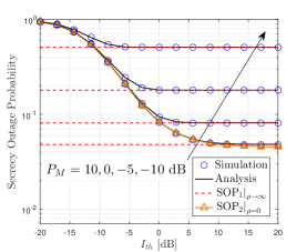
Figure 1: Secrecy outage probability versus $I_{th}$ for $K_{d}=K_{e}=K_{p}=10$, $\Delta_{d}=\Delta_{e}=\Delta_{p}=0.5$, $m_{d}=m_{e}=m_{p}=2.8$, $N_{0}=0$ dB, $\mu_{d}=\mu_{p}=1$, $\mu_{e}=0.1$, and $R_{s}=0.1$.

In Fig. 2, we can see that the SOP becomes better as $\mu_{e}$ decreases, due to the worse wiretap channel. The decreasing trend in SOP with respect to $\mu_{d}$ is shown in Figs. 2-3, where we can also see that the SOP is improved with decreasing $R_{s}$ (or increasing $K$), which can be explained by the fact that for a random variable $X$, the probability of $X\leq x$ becomes larger for larger $x$ (or the strength of the dominant waves of FTR fading channel grows).

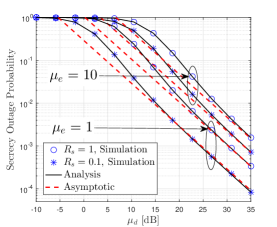
Figure 2: Secrecy outage probability versus $\mu_{d}$ for $K_{d}=K_{e}=K_{p}=5$, $\Delta_{d}=\Delta_{e}=\Delta_{p}=0.5$, $m_{d}=m_{e}=m_{p}=10.8$, $P_{M}=N_{0}=0$ dB, $\rho=-5$ dB, and $\mu_{p}=1$.

Further, the slopes in asymptotic results of Figs. 2-3 are fixed, regardless of any parameter setting, which reflects that the secrecy diversity order is always unity. The impact of all parameters on ASOP is reflected in the intercept on the abscissa axis (i.e., the secrecy array gain).

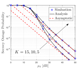
Figure 3: Secrecy outage probability versus $\mu_{d}$ for $K_{d}=K_{e}=K_{p}=K$, $\Delta_{d}=\Delta_{e}=\Delta_{p}=0.5$, $m_{d}=m_{e}=m_{p}=10.8$, $P_{M}=N_{0}=0$ dB, $\rho=-5$ dB, $R_{s}=3$, and $\mu_{e}=\mu_{p}=1$.

VI Conclusion

The analytical expression for the SOP was derived, which can be divided into two parts, i.e., ${\rm SOP}_{1}$ and ${\rm SOP}_{2}$. When $\rho=0$, our SOP becomes the SOP proposed by [13] without taking the maximal transmit power constraint into account. For $\rho\to\infty$, our SOP is reduced to the SOP in non-CRNs investigated in [11] where the impact of the primary network vanishes. when the SNR of $S-D$ link is sufficiently large, the ASOP shows that the secrecy diversity order is always unity regardless of any parameter setting. From the numerical results, we can conclude that the increase in $\rho$ (or $\mu_{d}$, $K_{d}$) and decrease in $\mu_{e}$ (or $R_{s}$) will lead to a lower SOP. However, due to the fact that the channel state is uncontrollable, the valid way for the transmitter to improve the SOP is to increase $\rho$ or decrease $R_{s}$.

References

• [1] L. Sboui, H. Ghazzai, Z. Rezki, and M.-S. Alouini, “Achievable rate of spectrum sharing cognitive radio multiple antenna channels,” IEEE Trans. Wireless Commun., vol. 14, no. 9, pp. 4847-4856, Sep. 2015.
• [2] A. Alsharoa, H. Ghazzai, and M.-S. Alouini, “Optimal transmit power allocation for MIMO two-way cognitive relay networks with multiple relays using AF strategy,” IEEE Wireless Commun. Lett., vol. 3, no. 1, pp. 30-33, Feb. 2014.
• [3] J. Lee, H. Wang, J. G. Andrews, and D. Hong, “Outage probability of cognitive relay networks with interference constraints,” IEEE Trans. Wireless Commun., vol. 10, no. 2, pp. 390-395, Feb. 2011.
• [4] M. Mezzavilla, M. Zhang, M. Polese, R. Ford, S. Dutta, S. Rangan, and M. Zorzi, “End-to-end simulation of 5G mmWave networks,” IEEE Commun. Surveys Tuts., vol. 20, no. 3, pp. 2237-2263, 3rd Quart. 2018.
• [5] J. M. Romero-Jerez, F. J. Lopez-Martinez, J. F. Paris, and A. J. Goldsmith, “The fluctuating two-ray fading model: Statistical characterization and performance analysis,” IEEE Trans. Wireless Commun., vol. 16, no. 7, pp. 4420-4432, Jul. 2017.
• [6] J. Zhang, W. Zeng, X. Li, Q. Sun, and K. P. Peppas,“New results on the fluctuating two-ray model with arbitrary fading parameters and its applications,” IEEE Trans. Veh. Technol., vol. 67, no. 3, pp. 2766-2770, Mar. 2018.
• [7] H. Zhao, Z. Liu, and M.-S. Alouini, “Different power adaption methods on fluctuating two-ray fading channels,” IEEE Wireless Commun. Lett., vol. 8, no. 2, pp. 592-595, Apr. 2019.
• [8] M. Bloch, J. Barros, M. R. D. Rodrigues, and S. W. McLaughlin, “Wireless information-theoretic security,” IEEE Trans. Inf. Theory, vol. 54, no. 6, pp. 2515-2534, Jun. 2008.
• [9] H. Zhao, Y. Tan, G. Pan, and Y. Chen, “Ergodic secrecy capacity of MRC/SC in single-input multiple-output wiretap systems with imperfect channel state information,” Front. Inform. Technol. Electron. Eng., vol. 18, no. 4, pp. 578-590, Apr. 2017.
• [10] L. Yang, M. O. Hasna, and I. S. Ansari, “Physical layer security for TAS/MRC systems with and without co-channel interference over $\eta$-$\mu$ fading channels,” IEEE Trans. Veh. Technol., vol. 67, no. 12, pp. 12421-12426, Dec. 2018.
• [11] W. Zeng, J. Zhang, S. Chen, K. P. Peppas, and B. Ai, “Physical layer security over fluctuating two-ray fading channels,” IEEE Trans. Veh. Technol., vol. 67, no. 9, pp. 8949-8953, Sep. 2018.
• [12] H. Lei, H. Zhang, I. S. Ansari, Z. Ren, G. Pan, K. A. Qaraqe, and M.-S. Alouini, “On secrecy outage of relay selection in underlay cognitive radio networks over Nakagami-$m$ fading channels,” IEEE Trans. Cog. Commun. Netw., vol. 3, no. 4, pp. 614-627, Dec. 2017.
• [13] Y. Liu, L. Wang, T. T. Duy, M. Elkashlan, and T. Q. Duong, “Relay selection for security enhancement in cognitive relay networks,” IEEE Wireless Commun. Lett., vol. 4, no. 1, pp. 46-49, Feb. 2015.
• [14] H. Zhao, Y. Tan, G. Pan, Y. Chen, and N. Yang, “Secrecy outage on transmit antenna selection/maximal ratio combining in MIMO cognitive radio networks,” IEEE Trans. Veh. Technol., vol. 65, no. 12, pp. 10236-10242, Dec. 2016.
• [15] I. S. Gradshteyn, I. M. Ryzhik, Table of Integrals, Series, and Products, 7th edition. Academic Press, 2007.