REVERBERATION MAPPING OF NARROW-LINE SEYFERT 1 GALAXY I ZWICKY 1: BLACK HOLE MASS

Abstract

We report results of the first reverberation mapping campaign of I Zwicky 1 during $2014$-$2016$, which showed unambiguous reverberations of the broad H$\beta$ line emission to the varying optical continuum. From analysis using several methods, we obtain a reverberation lag of $\tau_{\rm H\beta}=37.2^{+4.5}_{-4.9}\,$ days. Taking a virial factor of $f_{{}_{\rm BLR}}=1$, we find a black hole mass of $M_{\bullet}=9.30_{-1.38}^{+1.26}\times 10^{6}M_{\odot}$ from the mean spectra. The accretion rate is estimated to be $203.9_{-65.8}^{+61.0}\,L_{\rm Edd}c^{-2}$, suggesting a super-Eddington accretor, where $L_{\rm Edd}$ is the Eddington luminosity and $c$ is the speed of light. By decomposing Hubble Space Telescope images, we find that the stellar mass of the bulge of its host galaxy is $\log(M_{\rm bulge}/M_{\odot})=\rm 10.92\pm 0.07$. This leads to a black hole to bulge mass ratio of $\sim 10^{-4}$, which is significantly smaller than that of classical bulges and elliptical galaxies. After subtracting the host contamination from the observed luminosity, we find that I Zw 1 follows the empirical $R_{\rm BLR}\propto L_{5100}^{1/2}$ relation.

1 Introduction

Narrow-line Seyfert 1 galaxies (NLS1s) are thought to be a special subclass of active galactic nuclei (AGN). Compared to the broad-line Seyfert 1 galaxies, NLS1s have: (1) narrower Balmer lines (FWHM${}_{\rm H\beta}\lesssim 2000\rm\ km~{}s^{-1}$, by definition, where $\rm FWHM_{H\beta}$ is the full width at half maximum of the broad H$\beta$ emission line), (2) smaller intensity ratio of [O iii] $\lambda$5007, to H$\beta$ line ([O iii]/H$\beta<3$), (3) stronger optical Fe ii  multiplet emissions, and (4) usually steeper soft X-ray spectra and more rapid X-ray variability (Osterbrock & Pogge 1985; Goodrich 1989; Boroson & Green 1992; Boller et al. 1996; Sulentic et al. 2000; Wang et al. 2004). These distinctive properties of NLS1s can be explained by less massive black holes accreting with higher mass accretion rates (Boroson & Green 1992; Boller et al. 1996; Wang & Netzer 2003; Mathur & Grupe 2005; Grupe 2004; Peterson et al. 2004). Black holes in NLS1s are therefore undergoing fast growth through super-Eddington accretion (e.g., Kawaguchi et al. 2004; Zhang & Wang 2006; Wang & Zhang 2007). In the high-$z$ universe, such fast growth was suggested to be a possible way of forming supermassive black holes (Volonteri & Rees 2005; Wang et al. 2006; Mortlock et al. 2011; Bamnados et al. 2018). Moreover, these super-Eddington accreting massive black holes (SEAMBHs) have saturated luminosity predicted by slim accretion disk model (Abramowicz et al., 1988; Wang & Zhou, 1999) and could be used as a new kind of standard candle to study the expansion history of the high-$z$ Universe (Wang et al. 2013; Wang et al. 2014; Marziani & Sulentic 2014; Cai et al. 2018; Marziani et al. 2019) since they are quit common from low-$z$ to high-$z$ Universe (Du et al., 2016b; Negrete et al., 2018; Martínez-Aldama et al, 2018). Reliably measuring black hole mass of local super-Eddington AGNs greatly helps elucidate these issues.

The reverberation mapping (RM) technique is a powerful tool for measuring the mass of black hole in the centre of AGN (Peterson, 1993; Peterson et al., 2004; Peterson, 2014). The widely accepted scenario is that gas around the central back hole is photoionized by the continuum emissions from the accretion disk and emits the observed broad emission lines. This is known as broad-line regions (BLR). Because of the light-travel time from the central black hole to the BLR, the variation in the flux of emission lines will delay that of the continuum. RM-campaigns monitor the flux variations in the continuum and the broad emission lines to measure the lags between them. Thus the observed lags are regarded as a measurement of the radius of the BLR. Assuming that the motion of BLR gas is governed by the gravity of the black hole, the profiles of these lines would provide kinematic information of the BLR and the viral mass of the black hole can be estimated by

$$M_{\rm\bullet}=f_{{}_{\rm BLR}}\frac{\it R_{{}_{\rm BLR}}\it V_{{}_{\rm{FWHM}}}^{\rm 2}}{G},$$ (1)

where $f_{{}_{\rm BLR}}$ is the virial factor, $G$ is the gravitational constant, $R_{{}_{\rm BLR}}=c\times\tau_{\rm H\beta}$ is the emissivity-weighted size of the BLR emitting the broad H$\beta$ line, with $c$ the light speed and $V_{{}_{\rm FWHM}}$ the velocity of the BLR clouds inferred from the width of the broad H$\beta$ line. Recently, the mass of the black hole in 3C273 has been determined by another novel technique using GRAVITY on VLTI (Very Large Telescope Interferometer) (Sturm et al., 2018), and the result is in good agreement with that given by a 10-year RM-campaign (Zhang et al., 2018).

As one of the most famous NLS1s, I Zwicky 1 (PG 0050+124 or Mrk 1502, $z=0.061$; hereafter I Zw 1) is selected as one of candidates in our large RM-campaign focusing on AGNs with SEAMBHs (Du et al., 2014). I Zw 1 is a nearby and bright ($m_{V}=14.06\pm 0.05$ from Slavcheva-Mihova & Mihov 2011b) prototypical NLS1 (Schmidt & Green 1983; Osterbrock & Pogge 1985; Halpern & Oke 1987) with FWHM${}_{\rm H\beta}\simeq 1200\rm\ km~{}s^{-1}$, large relative strength of optical Fe ii  emission lines ($\mathcal{R}_{\rm Fe}=1.47$ from Boroson & Green 1992, where $\mathcal{R}_{\rm Fe}=F_{\rm Fe}/F_{\rm H\beta}$), weak intensity of [O iii]  line and a steep X-ray ($2-10$ keV) photon index ($\Gamma=2.15\pm 0.02$ from Gallo et al. 2007). Its Fe ii  spectrum is commonly used as a template to fit the optical and ultraviolet spectra of AGNs and quasars (Boroson & Green 1992; Vestergaard & Wilkes 2001; Véron-Cetty et al. 2004). Similar to other NLS1s, Hubble Space Telescope (HST) images show clearly that the host galaxy of I Zw 1 is a spiral galaxy with asymmetric knotty spiral arms (Slavcheva-Mihova & Mihov 2011a) consisting of young stellar populations and ongoing nuclear star formation activity (Hutchings & Crampton 1990; Scharwächter et al. 2007). It would be highly instructive to measure the black hole mass and accretion rate of I Zw 1 in order to understand the relation of its central engine to its host galaxy. As far as we know, only Giannuzzo et al. (1998) obtained seven epochs with a mean cadence of about 170 days to monitor optical variability of I Zw 1. This is not enough for RM measurements.

In this paper, we report results of the first RM campaign for I Zw 1. In §2, we describe the observations and data reduction. In §3, we analyze the light curves to measure the H$\beta$ time lags for black hole mass and fit the $HST$ images to separate the host component to test the empirical $R_{\rm BLR}$-$L_{5100}$ relation. Brief discussions are provided in §4. A summary is given in the last section. Throughout this work, we adopt a cosmology with $H_{0}=67\ \rm km~{}s^{-1}~{}Mpc^{-1}$, $\Omega_{\Lambda}=0.68$ and $\Omega_{\rm m}=0.32$ (Ade et al., 2014) .

2 OBSERVATIONS AND DATA REDUCTION

2.1 Observations

Our observations were performed from November 2014 to February 2016 using the Lijiang 2.4 m telescope of Yunnan Observatories, Chinese Academy of Sciences. A versatile instrument named Yunnan Faint Object Spectrograph and Camera (YFOSC) was adopted since it can switch from spectroscopy to photometry within one second (Du et al. 2014). During the spectroscopic observations, we used Grism 14, which covers the wavelength range of 3800$-$7200 Å, and a long slit with a fixed width of $2.^{\prime\prime}5$ to minimize flux loss caused by the different seeing conditions. The final spectral resolution was roughly $500\rm\ km~{}s^{-1}$. The spectral resolution was estimated by comparing the width of the [O iii]  line of the Lijiang spectrum with the one obtained from the Sloan Digital Sky Survey (Hu et al. 2015; du16). For accurate flux calibration, we adopted the method described by Maoz et al. (1990) and Kaspi et al. (2000), putting I Zw 1 and a nearby comparison star simultaneously in the long slit during the exposure. The comparison star (R.A._J2000 = 00:53:46.92, Dec._J2000 = + 12:39:56.8) is a stable G star without intrinsic changes, as confirmed from the photometric light curve shown in Appendix A. The position angle between the comparison star and I Zw 1 is $120^{\circ}$, and the angular distance is $3.4^{\prime}$. Flux changes caused by unstable weather can be corrected by the comparison star. To mitigate the influence of cosmic rays, we used two consecutive exposures with typical exposure time of 600 s each. Between the two exposures, we took an image to inspect whether I Zw 1 and the comparison star still sit in the middle of the slit. If not, we adjust the slit for realignment. Every night we also took two consecutive exposures of a spectrophotometric standard star. In order to minimise the impact of atmospheric differential refraction, we took spectra only when the air mass was $\lesssim 1.5$ (median air mass $\lesssim 1.3$ for our data). In addition, we also made $V$-band photometric observations to verify the accuracy of the spectral calibration. Three consecutive 90 s exposures were taken to reduce the impact of cosmic rays. We obtained 66 epochs of spectroscopic observations and 74 epochs of photometric observations for I Zw 1 during our campaign. The median cadence is $\simeq 4$ days.

2.2 Data reduction

All the spectroscopic and photometric data were reduced following standard methods using IRAF v2.16. For spectroscopic data, the extraction aperture was $8.^{\prime\prime}5$. Standard neon and helium lamps were used for wavelength calibration, and the comparison star was used for flux calibration, as described by Du et al. (2014). Here we briefly describe the method of flux calibration. (1) We used spectrophotometric standard stars to calibrate the spectra of the comparison star. (2) A fiducial spectrum of the comparison star was made from its flux-calibrated spectra taken over several nights under good weather conditions. The uncertainty of the absolute flux calibration was $\sim 10\%$ (Du et al. 2016a). (3) By comparing the observed spectrum of the comparison star to the calibrated fiducial spectrum, we obtained a sensitivity function for each exposure. (4) This sensitivity function was then used to calibrate the spectrum of I Zw 1. (5) We combined the separate exposures taken each night into a single-epoch spectrum for that night. This method can achieve an accuracy of $\sim 3\%$ in the calibrated spectra (Du et al. 2018), which is especially necessary for targets such as I Zw 1 and other SEAMBHs, whose [O iii]$\lambda 5007$ line tends to be too weak to be used for relative flux calibration, as conventionally practiced for RM (Foltz et al. 1981; Peterson et al. 1982).

For generating the photometric light curves of I Zw 1, six stars in the same fields were used to perform differential photometry. The radius of the aperture for I Zw 1 was $5.^{\prime\prime}1$, and that for the background was $8.^{\prime\prime}5-17.^{\prime\prime}0$. Specifically, for each exposure, we obtained the instrumental magnitudes of I Zw 1 and the six stars by IRAF. We calculated the differential magnitude between I Zw 1 and the mean of the six stars, and the uncertainties in all the instrumental magnitudes were propagated to the uncertainty in this differential magnitude. Then we averaged the differential magnitudes of the three exposures in the same night as the value of that individual night, and calculated a statistical uncertainty from the uncertainty of each exposure by error propagation. In addition, we calculated scatters between the differential magnitudes of the three exposures as the systematic uncertainty. The two uncertainties are added in quadrature as the final uncertainty of the differential magnitude in each night.

3 Data analysis and results

3.1 Light curves

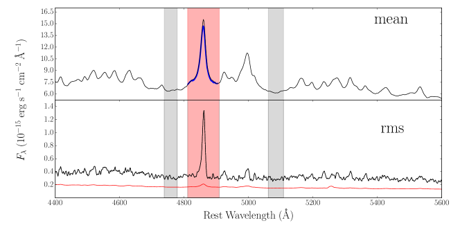
Figure 1: The mean and rms spectra for I Zw 1 from the 2014–2015 season. The grey bands are the continuum windows and the red band is the integration window for H$\beta$. The blue line is the narrow line-subtracted profile, and the red line is the mean of the errors of the individual spectra.

We use the following method to determine the 5100 Å flux density and the H$\beta$ flux. The 5100 Å flux is the median flux between 5075 and 5125 Å in the rest frame. The H$\beta$ flux is obtained by integrating the flux between 4810$-$4910 Å from the continuum-subtracted spectrum, while the continuum underlying the H$\beta$ line is determined by a linear interpolation between two continuum bands (4740-4790 Å and 5075-5125 Å). The continuum windows are selected to minimize the contamination from other emission lines, such as [O iii], Fe ii, and He ii. In Figure 1, we mark the window for the H$\beta$ line by the red band and the windows for the continuum by the grey bands. The measurement errors of the light curves come from both Poisson noise and systematic uncertainty. The systematic uncertainty arises from poor weather conditions, slit positioning, telescope tracking, and choice of continuum window. It can be estimated from the standard deviation of the residuals after subtracting a median-filtered, smoothed light curve. Table 1 lists the continuum flux density at 5100 Å and the H$\beta$ flux. Only 27 epochs are included from the 2014–2015 season, while 39 epochs are available for the 2015–2016 season. The seasonal gap between March 2015 and June 2015 is 120 days. We show the 5100 Å and H$\beta$ light curves during 2014–2016 in Figures 6i and 6j, respectively. The large errors of some points from 2015 June 20 to 2015 July 6 are caused by the bad weather during the rainy season of the Lijiang Station.

To improve the sampling of the continuum light curves, we used the $V$-band photometry data from ASAS-SN (All-Sky Automated Survey for SuperNovae). ASAS-SN is a long-term project aiming to monitor the entire visible sky to a depth of $V<17$ mag with a cadence of 2-3 days (Shappee et al., 2014; Kochanek et al., 2017). Between May 2014 and March 2016, ASAS-SN monitored I Zw 1 by two units of telescopes: ”Brutus”, deployed at the Hawaii station of the Las Cumbres Observatory, and ”Cassius”, deployed in Chile. 73 epochs for the 2014–2015 season, and 72 epochs for the 2015–2016 season, with enough S$/$N, were adopted here.

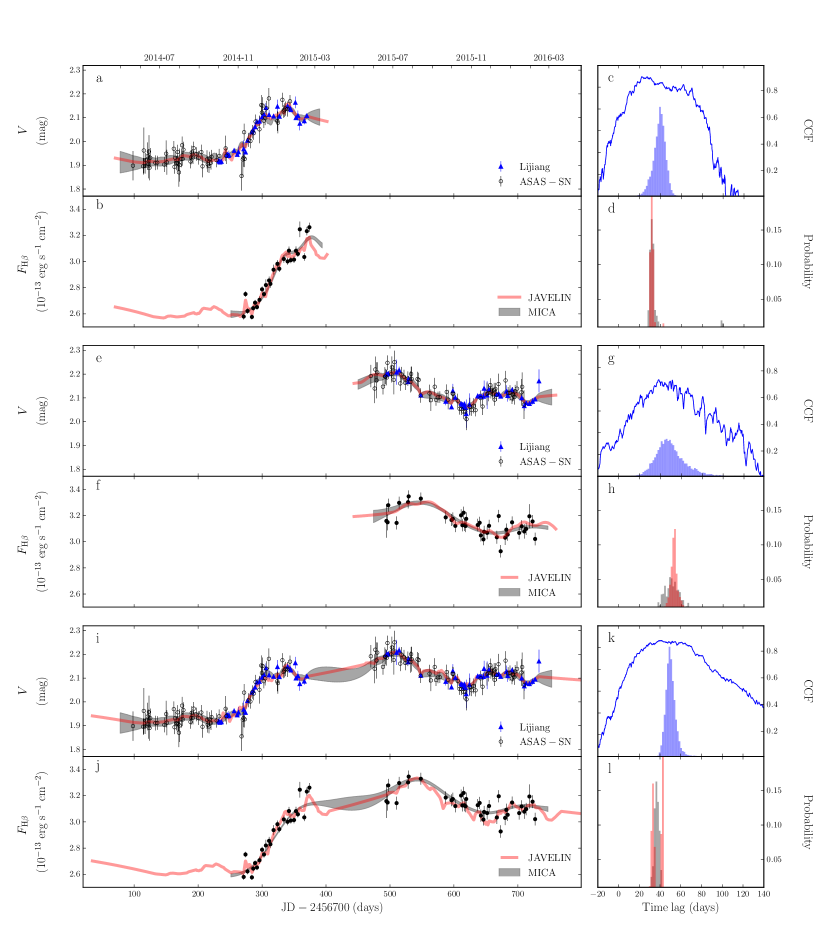
Figure 2: Light curves and results of correlation analysis using the photometric continuum light curves for I Zw 1. The left panels are light curves for different seasons. The red lines are the continuum light curve fitted by JAVELIN, while the gray bands are those fitted by MICA. The right panels show the correlation analysis. Panels (c, g, k) show ICCF results and panels (d, h, l) show results for MICA and JAVELIN for season 2014-2015, 2015-2016 and 2014-2016, respectively. The blue lines are the cross-correlation functions and the blue histograms are the cross correlation centroid distributions. The red histograms show the posterior probability of the time lags for JAVELIN, and the gray histograms show the corresponding one for MICA. JAVELIN, MICA and ICCF produce consistent lags for the same data.

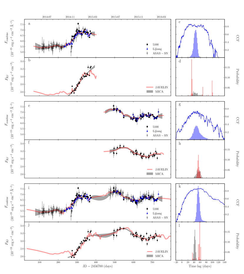
Figure 7: Light curves and results of correlation analysis using the combined continuum light curves for I Zw 1 (same as Figure 2).

We merge the $V$-band photometry data from the Lijiang and ASAS-SN into the 5100 Å light curves by applying a multiplicative scale factor and an additive flux adjustment, which are determined by a Markov-chain Monte Carlo (MCMC) implementation (Li et al. 2014; Du et al. 2015). The combined continuum light curves are shown in Figure 7i, which contain 136 epochs from the 2014–2015 season and 149 epochs from the 2015–2016 season. By combining ASAS-SN data, the continuum light curve shows an obvious structure for 2014-2015 season (shown in Figure 7i), which corresponds to that in the light curve of H$\beta$ and the seasonal gap is shortened to 94 days. However, as shown in Figure 7i, the 5100 Å light curves increase the scatter of the continuum light curve, so we merge only the $V$-band photometry data from ASAS-SN into the photometry data from Lijiang to obtain the final photometry continuum light curve shown in Figure 2i. The final photometric continuum light curve contains 109 and 110 epochs from the 2014–2015 and 2015–2016 seasons, respectively. We adopt the photometric continuum light curve to obtain the H$\beta$ lags in this paper. However, for comparison, we also show the results for the 5100 Å and the combined continuum light curves in Appendix B.

3.2 Variability characteristics

We use the methods described by  Rodríguez-Pascual et al. (1997) to calculate light curve characteristics of the continuum and the H$\beta$ emission line. The variability characteristics are given by

$$F_{\rm var}=\frac{(\sigma^{2}-\triangle^{2})^{1/2}}{\langle F\rangle},$$ (2)

where

$$\sigma^{2}=\sum_{i=1}^{N}\frac{(F_{i}-\langle F\rangle)^{2}}{(N-1)},\quad\triangle^{2}=\sum_{i=1}^{N}\frac{\Delta_{i}^{2}}{N},\quad\langle F\rangle=\sum_{i=1}^{N}\frac{F_{i}}{N},$$ (3)

and the error of $F_{\rm var}$ is given by

$$\sigma_{\rm var}=\frac{1}{F_{\rm var}}\left(\frac{1}{2\times N}\right)^{1/2}\frac{\sigma^{2}}{{\langle F\rangle}^{2}},$$ (4)

(Edelson et al., 2002), where $N$ is the total number of data, $F_{i}$ is the flux of the $i$-th observation, and $\Delta_{i}$ is the uncertainty of $F_{i}$. We use $F_{\rm var}^{5100}$, $F_{\rm var}^{\rm combine}$, $F_{\rm var}^{V}$ and $F_{\rm var}^{\rm H\beta}$ to denote the amplitude of the variation in the light curves of the 5100 Å continuum, the combined continuum, the photometry continuum and broad H$\beta$ line. Table 2 lists $F_{\rm var}^{5100}$, $F_{\rm var}^{\rm combine}$, $F_{\rm var}^{V}$ and $F_{\rm var}^{\rm H\beta}$ for the 2014–2015 data, 2015–2016 data, and 2014–2016 data, respectively. We find that $F_{\rm var}^{5100}$ , $F_{\rm var}^{\rm combine}$, $F_{\rm var}^{V}$ and $F_{\rm var}^{\rm H\beta}$ of I Zw 1 are clearly much smaller than that of other PG quasars (see Table 5 in Peterson et al. 1998 and Table 5 in Kaspi et al. 2000), by a factor of a few.

The mean and the rms spectra of I Zw 1 are calculated by

$$\bar{F}({\lambda})=\frac{1}{N}\sum_{i=1}^{N}F_{i}(\lambda);\quad S({\lambda})=\left\{\frac{1}{N-1}\sum_{i=1}^{N}\left[F_{i}(\lambda)-\bar{F}(\lambda)\right]^{2}\right\}^{1/2}.$$ (5)

We show the results for the 2014–2015 season in Figure 1. The [O iii]  line disappears in the rms spectrum, which implies that the spectral calibration is quite good. We also plot the mean of the error of the individual spectra (see the red line in Figure 1), which can be taken as the rms spectrum for the variance caused by noise only (Hu et al. 2016).

3.3 $H\beta$ lags

We employ three methods to calculate H$\beta$ lags: the interpolation cross-correlation function (ICCF; Gaskell & Sparke 1986; Peterson et al. 2004), JAVELIN (Zu et al. 2011), and MICA (Li et al. 2016). The ICCF method calculates the cross-correlation function (CCF) between the light curves of the continuum and H$\beta$ fluxes. The time lag is determined by measuring either the location $\tau_{\rm peak}$ of the CCF peak ($r_{\rm max}$) or the centroid $\tau_{\rm cent}$ of the points around the peak above a threshold $r\geq 0.8\ r_{\rm max}$. The associated uncertainties are estimated by the Monte Carlo flux randomization/random subset sampling (FR/RSS) method of Peterson et al. (1998) and are given at 63.8$\%$ confidence levels. Both JAVELIN and MICA are forward-modelling methods that use the damped random walk model (e.g., Kelly et al. 2009; Zu et al. 2011; Li et al. 2013) to delineate the variations of continuum light curves and directly infer the transfer functions of the BLR by presuming specific shapes of the transfer functions. JAVELIN adopts a top-hat transfer function, whereas MICA expresses the transfer function as a sum of a series of Gaussians. For simplicity, we only use one Gaussian in MICA. Accordingly, time lags are given by the center of the top-hat function in JAVELIN and the center of the Gaussian in MICA. Both JAVELIN and MICA use the MCMC technique to explore the model parameters of transfer functions. The time lags and the associated uncertainties are estimated as the expectation and standard deviation of the generated Markov chains, respectively.

In order to avoid potential biases introduced by seasonal gaps, we analyze the observations from the 2014–2015 and 2015–2016 seasons, as well as that for the whole campaign, separately (Figure 2). Figures 2a and 2b show the light curves for the photometric continuum and H$\beta$ emission line for the season 2014–2015. The light curves reconstructed by JAVELIN (red line) and MICA (gray band) are also superposed. Figure 2c shows the CCF and the cross-correlation centroid distribution (CCCD) for the season 2014–2015, and Figure 2d gives the posterior distributions of time lags obtained by JAVELIN (red) and MICA (gray). Figures 2e–2h are the same as Figures 2a–2d, but for the season 2015–2016, and the results for the entire 2014–2016 season are shown in Figures 2i–2l. Table 3 summarises the time lags determined by the above three methods. They are consistent to each other, within uncertainties.

We detect significant time lags with small uncertainties using the photometric light curves. The H$\beta$ time lags for the 2015–2016 data have large uncertainties (Figures 2g and 2h) because of the small variability amplitude and large flux dispersion of the light curves (see Figures 2e and 2f). In principle, JAVELIN and MICA can reconstruct the light curves during the large seasonal gaps, such that, for data for the whole campaign, the lags obtained by JAVELIN and MICA should be more robust than that derived by ICCF. We also find that the lags obtained using JAVELIN and MICA (Figure 2l) are more consistent with that obtained by ICCF for the 2014–2015 data (Figure 2c). From inspection of the CCF peak value $r_{\rm max}$, we adopt $\tau_{\rm cent}=37.2^{+4.5}_{-4.9}$ days from the ICCF analysis of the photometric continuum and H$\beta$ light curves from 2014$-$2015, and we use this value to calculate the black hole mass below.

3.4 Host galaxy

We use images obtained with the HST to study the host galaxy, in particular its overall morphology, bulge-to-total ratio, and bulge stellar mass. We also need to determine the degree to which the spectroscopically measured optical continuum is contaminated by host galaxy emission. The highest quality HST observations currently available are those obtained with the WFC3 camera on 2 November 2013 (GO-12903, PI: Luis C. Ho). I Zw 1 was observed for 300 s with the F438W filter (395–468 nm) in the UVIS channel and for 147 s with the F105W filter (901–1204 nm) in the IR channel. An additional short (40 s) F438W exposure was taken to warrant against saturation of the nucleus in the long exposure. These two filters were purposefully chosen to mimic $B$ and $I$ in the rest frame of I Zw 1, at the same time avoiding contamination from strong emission lines. The large wavelength separation between the two filters also offers the most leverage for constraining the stellar population (Section 5.2). To better sample the point-spread function (PSF), the long UVIS observation was taken with a three-point linear dither pattern, while the IR observation was taken with the four-point boxy dither pattern. To avoid overheads due to buffer dump, we employed the UVIS2-M1K1C-SUB 1k$\times$1k subarray for the UVIS channel and the IRSUB512 subarray for the IR channel, which resulted in a restricted field-of-view of 40^′′ $\times$40^′′ and 67^′′ $\times$67^′′, respectively.

Because of the sparseness of field stars in the vicinity of I Zw 1, the observations were conducted in GYRO mode, which, unfortunately, led to considerable degradation of the PSF of the dither-combined image generated from the standard data reduction pipeline. Instead, we use the DrizzlePac task AstroDrizzle (v1.1.16) to correct the geometric distortion, align the sub-exposures, perform sky subtraction, remove cosmic rays, and, finally combine the different exposures. The core of the AGN was severely saturated in the long F438W exposure, and it was replaced with an appropriately scaled version of the 40 s short exposure. Because the PSF of HST is undersampled, we broaden both our science and PSF images by convolving them with a Gaussian kernel so that the PSF can reach Nyquist sampling (Kim et al., 2008). This largely removes the sub-pixel mismatch of the core of the PSF and the smearing of the nucleus due to image drift.

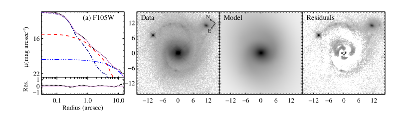
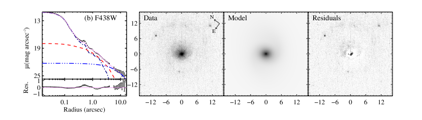
Figure 3: GALFIT decomposition for I Zw 1. The upper and lower panels show the fitting result of two different filters. In each row, 1D profile, 2D image of original data, best-fit model for the host (the AGN is excluded to better highlight the host) and residuals images are displayed. The 1D surface brightness profiles show the original data (black dots), the best fit (violet solid line), and the subcomponents (PSF in dark blue dot-dashed line, bulge in red dashed line and disk in blue dot-dashed line). The units of the images are in arcseconds. All images are on an asinh stretch.

The F105W image (Figure 3a) reveals a nearly face-on spiral galaxy with two dominant spiral arms. A bar-like structure may also be present. The F438W image (Figure 3b) is considerably shallower, but the host is still clearly detected. To extract quantitative measurements of the bulge, we use the program GALFIT (v3.0.5; Peng et al. 2002, 2010 ) to fit two-dimensional surface brightness distributions to the HST images. A crucial ingredient is the PSF, which will have a strong effect on the bright and active nucleus. Unfortunately, no suitably bright star is available to be used as the PSF within the limited field-of-view of the subarray WFC3 images. Instead, we generated a high-S/N stacked empirical PSF by combining a large number (24 for F105W and 57 for F438W) of bright, isolated, unsaturated stars observed during the course of other WFC3 programs. Extensive tests, consisting of fits to isolated bright stars, indicate that our stacked empirical PSF is far superior to synthetic PSFs generated from the TinyTim program (Krist & Hook, 1999), and it has higher S/N than the PSFs of individual stars. The reduced $\chi^{2}$ of the fits are $\sim$3 times larger for the TinyTim synthetic PSF. Comparison of empirical PSFs observed from different programs indicate that the WFC3 PSF does not vary significantly with time ($<$ 10%).

We concentrate first on obtaining the best global fit on the deeper F105W image, whose red wavelength is also more sensitive to the host. After much experimentation, we adopt a model with three components: a point source (represented by the PSF) for the nucleus, a bulge parameterized as a Sérsic (1968) function with index $n$, and an exponential disk (equivalent to a Sérsic function with $n=1$), with coordinate rotation turned on to fit the spiral arms. We could not obtain a robust solution that considers the faint, bar-like feature, and in the end we did not treat it. We use the $m=1$ Fourier mode of the disk, which is sensitive to lopsidedness, to gauge the degree of global asymmetry of the galaxy (see, e.g., Kim et al. 2008, 2017). The best model (Figure 3a) reveals a bulge with $n=1.73\pm 0.06$, formally but barely below the conventional threshold for pseudo-bulges ($n<2$; Fisher & Drory 2008) and an overall $B/T=0.52\pm{0.04}$. The disk is moderately asymmetric, with Fourier amplitude $a_{1}=0.11\pm{0.01}$. As the host is considerably weaker in the F438W image, we fit it keeping the structural parameters fixed to the values obtained from the F105W model, solving only for the magnitude.

The uncertainties of the decomposition are dominated by PSF mismatch in the nucleus. We estimate the effect of the PSF by generating variants of the empirical PSF by combining different subsets of stars, and then repeating the fit. The final error budget is the quadrature sum of these two contributions.

3.5 The $R-L$ relation

A proper evaluation of the $R-L$ relation must consider the influence of host galaxy contamination on the luminosity (Kaspi et al. 2000; Bentz et al. 2013). We use the decomposition of the HST images of I Zw 1 to estimate the contribution of the host galaxy within the spectral extraction aperture. The host flux at 5100 Å is transformed from the F438W magnitude with the IRAF task synphot, assuming a stellar population template with an age of 5.0 Gyr (Section 4.2), after correcting for redshift ($z=0.0611$) and Galactic reddening [$E(B-V)=0.057$ mag; Schlafly & Finkbeiner 2011] using the extinction curve of Cardelli et al. (1989).

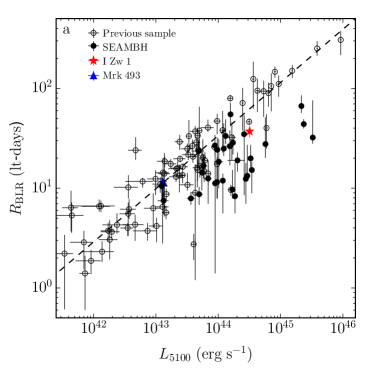
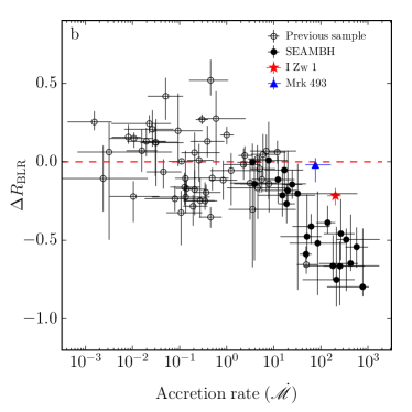
Figure 4: The (a) $R_{\rm BLR}-L_{5100}$ and (b) $\Delta R_{\rm BLR}-\dot{\mathscr{M}}$ plots, in which the open and solid points are from Bentz et al. (2013) and Du et al. (2018), respectively. The black dashed line is the classical $R-L$ relation (Bentz et al., 2013). The red star is I Zw 1, and the blue triangle is Mrk 493 from Hu et al. (2015); both are outliers in panel b. In panel b, the red dashed line is $\Delta R_{\rm BLR}=0$. I Zw 1 and Mrk 493 have $(\Delta R_{\rm BLR},\log\dot{\mathscr{M}})=(-0.22,2.31),(-0.02,1.88)$, respectively.

Table 4 lists the observed total, host galaxy, and AGN fluxes at 5100 Å. With an AGN luminosity of $L_{5100}=3.19\times 10^{44}\rm\ erg~{}s^{-1}$, I Zw 1 follows the empirical $R_{\rm BLR}-L_{5100}$ relation (Figure 4a).

4 Black hole mass and accretion rate

4.1 Mass

For measuring the black hole mass, the velocity of the BLR clouds are measured through the FWHM of the broad emission line (Equation 1). The narrow H$\beta$ component ($F_{\rm N}$) of I Zw 1 is too weak to be decomposed directly by spectral fitting even for the mean spectrum. Thus we subtract the $F_{\rm N}$ from the mean spectrum of the 2014–2015 season assuming $F_{\rm N}/F_{[\rm O\ {III}]}\simeq 0.1$ (Hu et al., 2012), where $F_{[\rm O\ {III}]}$ is the flux of [O iii]$\ \lambda 5007\$Å. Then we measure the FWHM directly from the narrow line-subtracted profile (blue line in Figure 1). The uncertainty is bracketed by assuming that $F_{\rm N}/F_{[\rm O\ {III}]}=0$ and 0.2. Correcting for an instrumental broadening of $500\rm\ km~{}s^{-1}$ (Hu et al. 2015; du16), $V_{{}_{\rm FWHM}}=\rm FWHM_{\rm H\beta}=1131_{-38}^{+35}\,\rm\ km~{}s^{-1}$ (Table 4). Adopting $\tau_{\rm H\beta}=37.2$ days and $f_{{}_{\rm BLR}}=1$, Equation (1) yields $M_{\bullet}=9.30_{-1.38}^{+1.26}\times 10^{6}\,M_{\odot}$. It is known that the observed kinematics of the BLR are generally influenced by inclination effects, which will lead to uncertainties of the virial factor (Krolik 2001; Collin et al. 2006). In principle, $f_{{}_{\rm BLR}}$ can be calibrated using the $M_{\bullet}-\sigma$ relation of inactive galaxies, and the current best estimates of $f_{{}_{\rm BLR}}$ are $1.3\pm 0.4$ for classical bulges and $0.5\pm 0.2$ for pseudo bulges, when $f_{{}_{\rm BLR}}$ is calibrated using FWHM based on mean spectra (Ho & Kim 2014). The host galaxy of I Zw 1 likely contains a pseudo bulge (Section 5.2). However, the large scatter of the $M_{\bullet}-\sigma$ relation of pseudo bulges (Kormendy & Ho 2013) introduces significant uncertainty into the estimate of $f_{{}_{\rm BLR}}$. For consistency with our previous work on SEAMBHs (Du et al., 2014, 2015; du16), we adopt $f_{{}_{\rm BLR}}=1.0$ (Netzer & Marziani 2010; Woo et al. 2013). We also estimate the black hole mass from the FWHM of the rms spectrum ($V_{{}_{\rm FWHM}}^{\rm rms}=\rm FWHM_{\rm H\beta}^{\rm rms}=606^{+28}_{-28}\,\rm\ km~{}s^{-1}$) using $f_{{}_{\rm BLR}}^{\rm rms}=1.12$ (Woo et al. 2015) and obtain $M_{\bullet}^{\rm rms}=2.99_{-0.48}^{+0.46}\times 10^{6}\,M_{\odot}$.

Meanwhile, polarized spectra of type 1 AGNs can provide invaluable information for estimating black hole masses. Considering electron scattering in the equatorial plane (Smith et al. 2005), a polarized spectrum is equivalent to a spectrum seen by an observer on the mid-plane. Thus, polarized spectra can yield more reliable estimates of the black hole mass (Afanasiev & Popovic 2015; Baldi et al. 2016; Songsheng & Wang 2018). For equatorial scattering of a BLR with a flattened geometry,

$$M_{\bullet}^{\prime}/M_{\odot}=f_{{}_{\rm BLR}}^{\prime}\frac{R_{{}_{\rm BLR}}V_{{}_{\rm FWHM}}^{\prime^{2}}}{G}=8.18\times 10^{6}\,\left(\frac{\tau_{\rm H\beta}}{37.2\rm\ days}\right)\left(\frac{V_{{}_{\rm FWHM}}^{\prime}}{2165\rm\ km~{}s^{-1}}\right)^{2},$$ (6)

where the virial factor $f_{{}_{\rm BLR}}^{\prime}\approx 0.24$ (with small uncertainty) and $V_{{}_{\rm FWHM}}^{\prime}$ is the FWHM of the broad-line profile in the polarized spectrum (Figure 3 in Songsheng & Wang 2018). Fortunately, a polarized spectrum of I Zw 1 for the H$\alpha$ emission line has been taken using the 6 m telescope of the Special Astrophysical Observatory of the Russian Academy of Science (L. Popović 2018, private communications). We find FWHM${}_{\rm H\alpha}^{\prime}=1983\rm\ km~{}s^{-1}$ from the polarized spectrum. The relation between the widths of H$\beta$ and H$\alpha$ in the polarized spectrum is unclear, but a reasonable assumption is that the same relation is followed as in the total spectrum if 1) both lines are scattered by the same population of electrons, and 2) the regions emitting H$\beta$ and H$\alpha$ lines are much smaller than the electron scattering region. So we use the relation FWHM${}_{\rm H\beta}=1.07\times 10^{3}\left({\rm FWHM_{H\alpha}}/10^{3}\rm\ km~{}s^{-1}\right)^{1.03}$ from Greene & Ho (2005), and obtained $V_{{}_{\rm{FWHM}}}^{\prime}=\rm{FWHM}_{\rm H\beta}^{\prime}=2165_{-182}^{+189}\rm\ km~{}s^{-1}$. This value needs to be tested observationally in the future. Equation (6) then yields $M_{\bullet}^{\prime}=8.18_{-1.75}^{+1.74}\times 10^{6}M_{\odot}$, which agrees remarkably well with the mass estimates based on the mean spectrum.

4.2 Accretion rates

Photon trapping causes the radiated luminosity of slim disks to saturate (Abramowicz et al. 1988; Wang & Zhou 1999; Mineshige et al. 2000). Under these conditions, the normal Eddington ratio $L_{\rm bol}/L_{\rm Edd}$ is very insensitive to the accretion rate and mainly depends on the black hole mass, where $L_{\rm Edd}$ is the Eddington luminosity and $L_{\rm bol}$ is the bolometric luminosity. This renders $L_{\rm bol}/L_{\rm Edd}$ unsuitable to indicate the accretion rate of SEAMBHs. As derived from the self-similar solution of slim disk, the photon trapping radius is $R_{\rm trap}\approx 72\,(\dot{\mathscr{M}}/80)R_{\rm g}$, where $R_{\rm g}=GM_{\bullet}/c^{2}$, and the radius emitting optical (5100 Å ) photons is $R_{\rm 5100}\approx 4.3\times 10^{3}m_{7}^{-1/2}R_{\rm g}$ (Wang & Zhou 1999), which is much larger than $R_{\rm trap}$. So optical photons can escape freely, and hence accretion rates can be reliably estimated from the formalism of the standard accretion disk model (Shakura & Sunyeav, 1973). The dimensionless accretion rate is defined as $\dot{\mathscr{M}}=\dot{M}_{\bullet}/L_{\rm Edd}c^{-2}$, with $\dot{M}_{\bullet}$ is the mass accretion rate. Given the 5100 Å luminosity and the black hole mass, $\dot{\mathscr{M}}=20.1(\ell_{44}/\cos i)^{3/2}m_{7}^{-2}$, where $\ell_{44}=L_{5100}/10^{44}\rm\ erg~{}s^{-1}$, $m_{7}=M_{\bullet}/10^{7}M_{\odot}$, and $i$ is the inclination angle between the line-of-sight and the accretion disk (Du et al., 2015). For I Zw 1, we have

$$\dot{\mathscr{M}}\approx 203.9\,\left(\frac{\ell_{44}}{3.19}\right)^{3/2}\left(\frac{m_{7}}{0.93}\right)^{-2},$$ (7)

yielding $\dot{\mathscr{M}}=203.9_{-65.8}^{+61.0}$, for $\rm cos\it i$ = 0.75. As discussed in du16, $\rm cos\it i$ = 0.75 is a reasonable mean value for type 1 AGNs. If we take $\Delta\rm\ log\ cos\ \it i\lesssim\rm 0.1$, then the uncertainty on $\dot{\mathscr{M}}$ due to $i$ will be $\Delta\ \rm log\ \dot{\mathscr{M}}=1.5\ \Delta\ log\ cos\ \it i\lesssim\rm 0.15$. The inclination also has insignificant effect on the observed width of the broad emission lines $V_{{}_{\rm{FWHM}}}$ . If we know the Keplerian velocity $V_{{}_{\rm K}}$ and the height $H_{\rm BLR}$ of the flattened BLR, by the zeroth-order approximation, $V_{{}_{\rm FWHM}}\approx\left[\left({H_{\rm BLR}}/{R}\right)^{2}+\sin^{2}i\right]^{\rm 1/2}\ V_{{}_{\rm K}}$. By detailed modeling of RM data, Li et al. (2013) and Pancoast et al. (2014) suggest ${H_{\rm BLR}/R}\sim 1$, thus ${\rm sin\it i}\leq{H_{\rm BLR}/R}$, which implies the inclination has insignificant influence on $V_{{}_{\rm{FWHM}}}$, hence $M_{\bullet}$ and then ${\dot{\mathscr{M}}}$. The high dimensionless accretion rate indicates that I Zw 1 is a SEAMBH. Note that the accretion rate could be even higher by a factor of $\sim$ 10 than the present, if the FWHM obtained from rms spectrum are used in the calculation.

5 Discussion

5.1 The $R-L$ relation

There is growing evidence that the empirical $R_{\rm BLR}$-$L_{5100}$ relation does not apply to SEAMBHs. For a given luminosity, SEAMBHs tend to have a shorter H$\beta$ lag, suggesting that the size of the BLR is related not only to luminosity but also to the accretion rate (Du et al., 2015; du16; Du et al., 2018). According to the unified scaling relation for sub- and super-Eddington AGNs suggested by du16,

$$R_{\rm BLR}=29.6\,\ell_{44}^{0.56}\min\left[1,\left(\frac{\dot{\mathscr{M}}}{11.2}\right)^{-0.52}\right]\ {\rm lt\verb|-|day},$$ (8)

I Zw 1 is predicted to have an H$\beta$ delay of 12.5 days, which is much shorter than our measured value of 37.2 days. Unlike other SEAMBHs, I Zw 1 actually follows the standard $R_{\rm BLR}$-$L_{5100}$ relation and does not show an obvious shortened H$\beta$ lag (Figure 4a). Defining the deviation $\Delta R_{\rm BLR}\equiv\log(R_{\rm BLR}/R_{\rm R-L})$, where $R_{\rm R-L}$ is given by the empirical $R_{\rm BLR}-L_{5100}$ relation, Figure 4b plots $\Delta R_{\rm BLR}$ versus $\dot{\mathscr{M}}$. I Zw 1 deviates from the trend defined by most SEAMBHs. So does Mrk 493. The reasons for these outliers are unclear. One possibility is that some lags are too short to detect, given the current observation cadence. Within the SEAMBH framework described by Wang et al. (2014b) and Du et al. (2018), there are two BLRs: a normal one unshadowed, and another shadowed by the inner part of the disk and much closer to the central black hole. The emissivity-weighted gas distribution yields two peaks in the transfer function, corresponding to the unshadowed and shadowed BLRs respectively. Such a two-region BLR scenario gets supported from a recent modelling of the observed RM data in Mrk 142 by Li et al. (2018), which constructed flexible one-region and two-region models that included the spatial distribution and anisotropic emissivity of BLR clouds. They found that the two-region model is preferrable to the one-region model. However, the observed H$\beta$ lag depends on the data quality, especially the cadence. For example, low cadence will smooth the light curves and yields a single broad peak in the CCF, although there are two peaks in the transfer function. To measure the potential shorter lag, campaign with higher cadence than the present are being planned for getting detailed BLRs of I Zw 1 and Mrk 493 as done in Mrk 142.

5.2 Black hole and bulge stellar masses

The GALFIT decomposition of the HST images of I Zw 1 yields a bulge magnitude $17.23\pm 0.04$ mag in F438W and $14.07\pm 0.07$ mag in F105W. We apply $K$-correction to convert the HST-based magnitudes to rest-frame magnitudes in $B$ and $I$. We generate a series of template spectra with ages spanning 1 to 12 Gyr, adopting a Bruzual & Charlot (2003) models with solar metallicity, a Chabrier (2003) stellar initial mass function, and an exponentially decreasing star formation history with a star formation timescale of 0.6 Gyr. After accounting for Galactic extinction and redshift, we convolve the spectra with the response functions of the HST filters and generate synthetic F438W and F105W magnitudes. The observed bulge color of F438W$-$F105W = $3.16\pm 0.08$ mag is best matched with a stellar population of age $5.0^{+1.0}_{-0.5}$ Gyr, resulting in rest-frame $M_{I}=-22.70\pm 0.07$ mag and $B-I=1.96\pm 0.09$ mag. From Table 4 of Bell & de Jong (2001), we derived $M_{\mathrm{bulge}}=10^{11.18\pm 0.07}M_{\odot}$, assuming solar metallicity and a Salpeter (1955) initial mass function. A Chabrier initial mass function gives 45% less mass (Longhetti & Saracco, 2009), and therefore $M_{\mathrm{bulge}}={10^{10.92\pm 0.07}}M_{\odot}$.

For $M_{\bullet}=10^{6.97}M_{\odot}$, $M_{\bullet}/M_{\mathrm{bulge}}\approx 10^{-4}$, which is lower by a factor of $\sim 50$ than the value inferred from the $M_{\bullet}-M_{\rm bulge}$ relation for classical bulges and elliptical galaxies, but lies within the large scatter and lower ratios found for pseudo bulges (Kormendy & Ho, 2013). I Zw 1 very likely hosts a pseudo bulge, in view of its relatively low Sérsic index of $n=1.73\pm 0.06$ (Fisher & Drory 2008) and evidence for recent (see discussion above) and ongoing (Scharwächter et al., 2007) nuclear star formation.

6 SUMMARY

The first campaign for I Zw 1 had been performed by the SEAMBH project during 2014$-$2016. The main conclusions are as follows.

1. Applying the ICCF centroid method for the 2014$-$2015 data, the H$\beta$ time lag is $\tau_{\rm H\beta}=37.2^{+4.5}_{-4.9}$ days, and it follows the empirical $R_{\rm BLR}-L_{5100}$ relationship.

2. Using the total mean spectra, we calculate a black hole mass of $M_{\bullet}=9.30_{-1.38}^{+1.26}\times 10^{6}\,M_{\odot}$ and an accretion rate of $203.9_{-65.8}^{+61.0}\ L_{\rm Edd}c^{-2}$. From the rms spectrum, we estimate $M_{\bullet}=2.99_{-0.48}^{+0.46}\times 10^{6}\,M_{\odot}$, whereas the polarized spectrum yields $M_{\bullet}=8.18_{-1.75}^{+1.74}\times 10^{6}\,M_{\odot}$.

3. We derive the stellar for the bulge of the host galaxy from detailed decomposition of HST images. We find a mass ratio of $M_{\bullet}/M_{\rm bulge}\approx 10^{-4}$, much lower than that for nearby inactive classical bulges and elliptical galaxies.

I Zw 1 is famous for its strong and narrow Fe ii lines; however, the current data do not allow us to successfully measure a lag for Fe ii. We are in the process of scheduling a new monitoring campaign with improved cadence and homogeneity in observation more favourable for detecting Fe ii lags.

Table 1: Continuum and H$\beta$ Fluxes

JD-		$F_{5100}$		$F_{\rm H\beta}$
2456700+		$(10^{-15}\rm\ erg~{}s^{-1}~{}cm^{-2}~{}\AA^{-1})$		$(10^{-13}\rm\ erg~{}s^{-1}~{}{\rm cm^{-2}})$
271.28		6.11 $\pm$ 0.06		2.58 $\pm$ 0.02
274.08		6.44 $\pm$ 0.07		2.75 $\pm$ 0.02
277.27		6.40 $\pm$ 0.08		2.62 $\pm$ 0.02
284.12		6.44 $\pm$ 0.06		2.58 $\pm$ 0.02
286.19		6.44 $\pm$ 0.06		2.64 $\pm$ 0.02

Note. — $F_{5100}$ is the flux at $(1+z)$5100 Å  in the observed frame.

(This table is available in its entirety in machine-readable form.)

Table 2: Characteristics of the Light Curves

Parameter	$2014-2015$	$2015-2016$	$2014-2016$
$N_{5100}$	27	39	66
$N_{V}$	109	110	219
$N_{\rm combine}$	136	149	285
$N_{\rm H_{\beta}}$	27	39	66
$F_{\rm var}^{5100}(\%)$	$3.3\pm 0.6$	$4.1\pm 0.6$	$4.3\pm 0.4$
$F_{\rm var}^{V}(\%)$	$4.2\pm 0.4$	$1.6\pm 0.3$	$4.3\pm 0.3$
$F_{\rm var}^{\rm combine}(\%)$	$9.3\pm 0.7$	$3.7\pm 0.4$	$8.5\pm 0.4$
$F_{\rm var}^{\rm H\beta}(\%)$	$6.8\pm 1.0$	$2.4\pm 0.4$	$5.9\pm 0.5$

Table 3: Results of Correlation Analysis

Parameter	$2014-2015$		$2015-2016$		$2014-2016$
	Observed	Rest-frame	Observed	Rest-frame	Observed	Rest-frame
$\rm H\beta$ vs $V$-band
$r_{\rm max}$	0.91	0.91	0.73	0.73	0.88	0.88
$\tau_{\rm cent}$(days)	39.5${}^{+4.9}_{-6.1}$	37.2${}^{+4.5}_{-4.9}$	48.2${}^{+15.2}_{-11.4}$	45.4${}^{+14.3}_{-10.7}$	49.8${}^{+4.7}_{-4.0}$	46.9${}^{+4.5}_{-3.7}$
$\tau_{\rm peak}$(days)	27.8${}^{+14.1}_{-5.8}$	26.2${}^{+13.3}_{-5.5}$	48.4${}^{+19.9}_{-14.8}$	45.6${}^{+18.8}_{-13.9}$	46.2${}^{+14.4}_{-7.5}$	43.6${}^{+13.6}_{-7.0}$
$\tau_{\rm JAVELIN}$(days)	31.6${}^{+1.4}_{-0.8}$	29.8${}^{+1.3}_{-0.8}$	53.3${}^{+5.4}_{-4.1}$	50.2${}^{+5.1}_{-3.9}$	34.9${}^{+7.6}_{-2.5}$	32.9${}^{+7.2}_{-2.4}$
$\tau_{\rm MICA}$(days)	36.7${}^{+16.1}_{-16.1}$	34.6${}^{+15.2}_{-15.2}$	50.9${}^{+10.3}_{-10.3}$	48.0${}^{+9.7}_{-9.7}$	36.9${}^{+2.5}_{-2.5}$	34.8${}^{+2.4}_{-2.4}$

Note. — $\tau_{\rm cent}$ and $\tau_{\rm peak}$ are lags from ICCF analysis with the corresponding correlation coefficient ($r_{\rm max}$), while $\tau_{\rm JAVELIN}$ is the lag from JAVELIN and $\tau_{\rm MICA}$ is the lag from MICA.

Table 4: Results of the RM Campaign in the 2014–2015 Season

Parameter	Value
$F_{\rm obs}$(5100 Å)	$6.62_{-0.28}^{+0.28}\times 10^{-15}\ \rm\ erg~{}s^{-1}~{}cm^{-2}~{}\AA^{-1}$
$F_{\rm gal}$(5100 Å)	$1.50_{-0.16}^{+0.16}\times 10^{-15}\ \rm\ erg~{}s^{-1}~{}cm^{-2}~{}\AA^{-1}$
$F_{\rm AGN}$(5100 Å)	$5.12_{-0.44}^{+0.44}\times 10^{-15}\ \rm\ erg~{}s^{-1}~{}cm^{-2}~{}\AA^{-1}$
$L_{5100}$(AGN)	$3.19_{-0.27}^{+0.27}\times 10^{44}\ \rm\ erg~{}s^{-1}$
FWHM(mean)	$1131_{-38}^{+35}\,\rm\ km~{}s^{-1}$
FWHM(rms)	$606_{-28}^{+28}\,\rm\ km~{}s^{-1}$
$M_{\bullet}$	$9.30_{-1.38}^{+1.26}\times 10^{6}M_{\odot}$ (from the mean spectrum)
	$2.99_{-0.48}^{+0.46}\times 10^{6}M_{\odot}$ (from the rms spectrum)
	$8.18_{-1.75}^{+1.74}\times 10^{6}M_{\odot}$ (from the polarized spectrum)
$\dot{\mathscr{M}}$	$203.9^{+61.0}_{-65.8}$

Note. — $F_{\rm obs}$ and $F_{\rm gal}$ are the observed and host galaxy flux densities at $(1+z)5100$ Å in the observed frame. $L_{5100}$ is the mean AGN luminosity $\lambda L_{\lambda}$ at rest-frame 5100 $\rm\AA$ after subtracting the host galaxy and correcting for Galactic extinction.

Appendix A Light curve of the comparison star

In order to check the stability of the comparison star during the campaign, we obtain its photometric light curve using five stars in the same field to perform differential photometry. The light curve of the comparison star is shown in Figure 5. The standard deviation is 1.9$\%$ , demonstrating that the comparison star does not vary significantly.

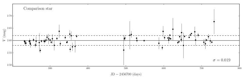
Figure 5: The photometry light curves for the comparison star of I Zw 1. The solid line marks the average value and the dashed lines mark the $\pm 1\sigma$ standard deviation.

Appendix B Light curves and H$\beta$ lags

Figure 6 and 7 show the results of the correlation analysis using the 5100 Å and combined continuum light curves. For the 2014–2015 data, the H$\beta$ time lag cannot be constrained well solely using the 5100 Å light curves. As shown in Figures 6c and 6d, the CCF is very spiky and the posterior distributions of the time lags obtained by JAVELIN and MICA are not well-defined. This may be caused by the short duration and the large scatter of the continuum light curves. As shown in Tables 5 and 3, the uncertainty of the time lags derived using only the photometry continuum light curves is smaller than that using the combined continuum light curves.

In Figure 8, we show the ASAS-SN light curve of I Zw 1 from 2012 to the end of 2018. Generally, the source was less variable in those 7 years except for the period from 2014-07 to 2016-01. During the whole period, the variability of the continuum flux is $F_{\rm var}(\%)=0.63\pm 0.02$, which is much smaller than that of the 2014-2016 period. We were lucky in this SEAMBH campaign and captured the largest variations in this period. Figure 8 shows that it is less variable again after the present campaign, which implys that we may need a longer waiting for sharp variations. Higher cadence than 2-3 days is also necessary for more details of the BLR structure. On the other hand, the long-term stability of I Zw 1 supports SEAMBHs as cosmic candles for cosmology (Wang et al., 2013, 2014; Cai et al., 2018).

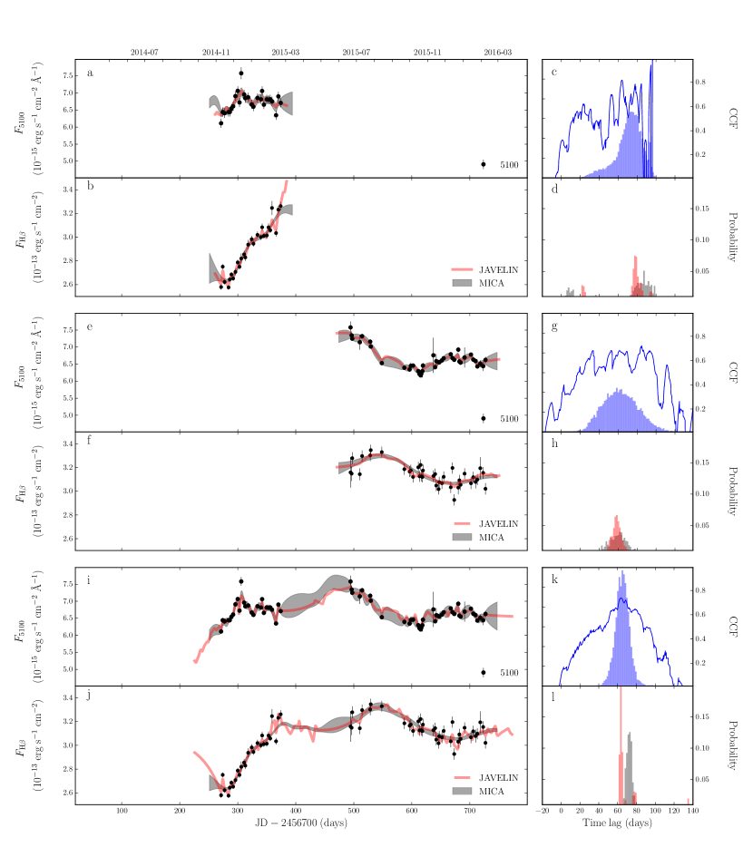
Figure 6: Light curves and results of correlation analysis using the 5100 Å continuum light curves for I Zw 1 (same as Figure 2).

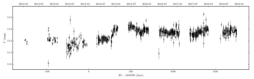
Figure 8: The 7-year $V-$band light curves of I Zw 1 monitored by ASAS-SN. It shows that I Zw 1 is quite stable in long-term. This makes it difficult to capture reverberation of the H$\beta$ line.

Table 5: Results of Correlation Analysis

Parameter	$2014-2015$		$2015-2016$		$2014-2016$
	Observed	Rest-frame	Observed	Rest-frame	Observed	Rest-frame
$\rm H\beta$ vs $F_{5100}$
$r_{\rm max}$	–	–	0.72	0.72	0.74	0.74
$\tau_{\rm cent}$(days)	73.3${}^{+11.7}_{-14.8}$	69.1${}^{+11.0}_{-13.9}$	61.9${}^{+19.8}_{-18.2}$	58.3${}^{+18.7}_{-17.2}$	65.2${}^{+6.9}_{-7.0}$	61.4${}^{+6.5}_{-6.6}$
$\tau_{\rm peak}$(days)	87.7${}^{+8.9}_{-20.4}$	82.7${}^{+8.4}_{-19.2}$	57.9${}^{+33.5}_{-24.0}$	54.6${}^{+31.6}_{-22.6}$	64.0${}^{+7.9}_{-4.1}$	60.3${}^{+7.4}_{-3.8}$
$\tau_{\rm JAVELIN}$(days)	78.0${}^{+7.4}_{-47.8}$	73.5${}^{+7.0}_{-45.0}$	59.1${}^{+10.4}_{-7.0}$	55.7${}^{+9.8}_{-6.6}$	64.0${}^{+13.3}_{-1.2}$	60.3${}^{+12.5}_{-1.1}$
$\tau_{\rm MICA}$(days)	66.2 ${}^{+34.9}_{-34.9}$	62.4${}^{+32.9}_{-32.9}$	59.9${}^{+12.5}_{-12.5}$	56.5${}^{+11.8}_{-11.8}$	72.1${}^{+2.9}_{-2.9}$	67.9${}^{+2.7}_{-2.7}$
$\rm H\beta$ vs $F_{\rm combine}$
$r_{\rm max}$	0.86	0.86	0.75	0.75	0.87	0.87
$\tau_{\rm cent}$(days)	44.1${}^{+5.1}_{-5.5}$	41.6${}^{+4.8}_{-5.2}$	48.9${}^{+15.0}_{-10.4}$	46.1${}^{+14.1}_{-9.8}$	54.2${}^{+5.0}_{-4.1}$	51.1${}^{+4.6}_{-3.9}$
$\tau_{\rm peak}$(days)	39.3${}^{+22.7}_{-13.0}$	37.6${}^{+21.4}_{-12.3}$	49.2${}^{+18.7}_{-14.4}$	46.4${}^{+17.6}_{-13.6}$	57.4${}^{+7.0}_{-13.1}$	54.1${}^{+6.6}_{-12.4}$
$\tau_{\rm JAVELIN}$(days)	33.1${}^{+65.2}_{-1.5}$	31.2${}^{+61.4}_{-1.4}$	54.0${}^{+5.4}_{-3.0}$	50.9${}^{+4.8}_{-2.8}$	57.9${}^{+1.0}_{-6.5}$	54.6${}^{+1.0}_{-6.1}$
$\tau_{\rm MICA}$(days)	45.5${}^{+22.8}_{-22.8}$	42.9${}^{+21.5}_{-21.5}$	53.6${}^{+10.5}_{-10.5}$	50.5${}^{+9.9}_{-9.9}$	42.2${}^{+2.7}_{-2.7}$	39.8${}^{+2.5}_{-2.5}$

Note. — $\tau_{\rm cent}$ and $\tau_{\rm peak}$ are lags from ICCF analysis with the corresponding correlation coefficient ($r_{\rm max}$), while $\tau_{\rm JAVELIN}$ is the lag for JAVELIN and $\tau_{\rm MICA}$ is the lag for MICA.

References

- Abramowicz et al. (1988) Abramowicz, M., Czerny, B., Lasota, J. & Szuszkiewicz, E. 1988, ApJ, 332, 646
- Ade et al. (2014) Ade, P.A.R., Arnaud, M., et al.(Planck Collaboration)2014, A&A, 571.A31
- Afanasiev & Popovic (2015) Afanasiev, V. L. & Popović, L. 2015, ApJ, 800, L35
- Baldassare et al. (2017) Baldassare, V. F., Reines, A. E., Gallo, E., & Greene, J. E. 2017, ApJ, 850, 196
- Baldi et al. (2016) Baldi, R. D., Capetti, A., Robinson, A., Laor, A., & Behar, E. 2016, MNRAS, 458, L69
- Bamnados et al. (2018) Banados, E. et al. 2018, Nature, 553, 473
- Bell & de Jong (2001) Bell, E. F., & de Jong, R. S. 2001, ApJ, 550, 212
- Bentz et al. (2013) Bentz, M. C., Denney, K. D., Grier, C. J., et al. 2013, ApJ, 767, 149
- Binney & Merrifield (1998) Binney, J., & Merrifield, M. 1998, Galactic astronomy / James Binney and Michael Merrifield. Princeton, NJ : Princeton University Press, 1998. (Princeton series in astrophysics) QB857 .B522 1998
- Blandford & McKee (1982) Blandford, R. D., & McKee, C. F. 1982, ApJ, 255, 419
- Boller et al. (1996) Boller, T., Brandt, W. N., & Fink, H. 1996, A&A, 305, 53
- Boroson & Green (1992) Boroson, T. A., & Green, R. F. 1992, ApJS, 80, 109
- Bruzual & Charlot (2003) Bruzual, G., & Charlot, S. 2003, MNRAS, 344, 1000
- Cai et al. (2018) Cai, R.-G., Guo, Z.-K., Huang, Q.-G. & Yang, T. 2018, Phys. Rev. D, 97, 123502
- Cardelli et al. (1989) Cardelli, J. A., Clayton, G. C., & Mathis, J. S. 1989, ApJ, 345, 245
- Chabrier (2003) Chabrier, G. 2003, PASP, 115, 763
- Collin et al. (2006) Collin, S., Kawaguchi, T., Peterson, B. M., & Vestergaard, M. 2006, A&A, 456, 75
- Du et al. (2014) Du, P., Hu, C., Lu, K.-X., et al. 2014, ApJ, 782, 45
- Du et al. (2015) Du, P., Hu, C., Lu, K.-X., et al. 2015, ApJ, 806, 22
- Du et al. (2016a) Du, P., Lu, K.-X., Zhang, Z.-X., et al. 2016a, ApJ, 825, 126
- Du et al. (2016b) Du, P., Wang, J.-M., Hu, C., et al. 2016b, ApJ, 818, L14
- Du et al. (2017) Du, P., Wang, J.-M., & Zhang, Z.-X. 2017, ApJ, 840, L6
- Du et al. (2018) Du, P., Zhang, Z.-X., Wang, K., et al. 2018, ApJ, 856, 6
- Edelson et al. (2002) Edelson, R., Turner, T. J., Pounds, K. et al. 2002, ApJ, 568, 610
- Fisher & Drory (2008) Fisher, D. B., & Drory, N. 2008, AJ, 136, 773
- Foltz et al. (1981) Foltz, C. B., Peterson, B. M., Cariotti, E. R., et al. 1981, ApJ, 250, 508
- Gadotti (2009) Gadotti, D. A. 2009, MNRAS,
- Gallo et al. (2007) Gallo, L. C., Brandt, W. N., Costantini, E., & Fabian, A. C. 2007, MNRAS, 377, 1375
- Gao & Ho (2017) Gao, H., & Ho, L. C. 2017, ApJ, 845, 114
- Gaskell & Sparke (1986) Gaskell, C. M., & Sparke, L. S. 1986, ApJ, 305, 175
- Giannuzzo et al. (1998) Giannuzzo, M. E., Mignoli, M., Stirpe, G. M., & Comastri, A. 1998, A&A, 330, 894
- Goodrich (1989) Goodrich, R. W. 1989, ApJ, 342, 224
- Graham et al. (2011) Graham, A. W., Onken, C. A., Athanassoula, E., & Combes, F. 2011, MNRAS, 412, 2211
- Greene & Ho (2005) Grenne, J. & Ho, L. C. 2005, ApJ, 630, 122
- Grupe (2004) Grupe, D. 2004, AJ, 127, 1799
- Halpern & Oke (1987) Halpern, J. P., & Oke, J. B. 1987, ApJ, 312, 91
- Ho & Kim (2014) Ho, L. C., & Kim, M. 2014, ApJ, 789, 17
- Hu (2009) Hu, J. 2009, arXiv:0908.2028
- Hu et al. (2008) Hu, C., Wang, J.-M., Ho, L. C., et al. 2008, ApJ, 687, 78-96
- Hu et al. (2012) Hu, C., Wang, J.-M., Ho, L. C., et al. 2012, ApJ, 760, 126
- Hu et al. (2015) Hu, C., Du, P., Lu, K.-X. et al. 2015, ApJ, 804, 138
- Hu et al. (2016) Hu, C., Wang, J.-M., Ho, L. C., et al. 2016, ApJ, 832, 197
- Hutchings & Crampton (1990) Hutchings, J. B., & Crampton, D. 1990, AJ, 99, 37
- Kaspi et al. (2000) Kaspi, S., Smith, P. S., Netzer, H., et al., 2000, ApJ, 533, 631
- Kawaguchi et al. (2004) Kawaguchi, T., Aoki, K., Ohta, K. & Collin, S. 2004, A&A, 420, L23
- Kelly et al. (2009) Kelly, B. C., Bechtold, J., & Siemiginowska, A., 2009, ApJ, 698, 895-910
- Kim et al. (2008) Kim, M., Ho, L. C., Peng, C. Y., Barth, A. J., & Im, M. 2008, ApJS, 179, 283
- Kim et al. (2008) Kim, M., Ho, L. C., Peng, C. Y., et al. 2008, ApJ, 687, 767
- Kim et al. (2017) Kim, M., Ho, L. C., Peng, C. Y., Barth, A. J., & Im, M. 2017, ApJS, 232, 21
- Kinney et al. (1996) Kinney, A. L., Calzetti, D., Bohlin, R. C., et al. 1996, ApJ, 467, 38
- Kochanek et al. (2017) Kochanek, C. S., Shappee, B. J., Stanek, K. Z., et al. 2017, PASP, 129, 104502
- Kormendy & Ho (2013) Kormendy, J., & Ho, L. C. 2013, ARA&A, 51, 511
- Kormendy & Richstone (1995) Kormendy, J., & Richstone, D. 1995, ARA&A, 33, 581
- Krist & Hook (1999) Krist, J.,& Hook, R.1999, The Tiny Time User’s Guide (Baltimore: STScI)
- Krolik (2001) Krolik, J. H. 2001, ApJ, 551, 72
- Li et al. (2013) Li, Y.-R., Wang, J.-M., Ho, L. C., Du, P., & Bai, J.-M. 2013, ApJ, 779, 110
- Li et al. (2014) Li, Y.-R., Wang, J.-M., Hu, C., Du, P., & Bai, J.-M. 2014, ApJ, 786, L6
- Li et al. (2016) Li, Y.-R., Wang, J.-M., & Bai, J.-M. 2016, ApJ, 831, 206
- Li et al. (2018) Li, Y.-R., Songsheng, Y.-Y., Qiu, J. et al. (SEAMBH collaboration), 2018, ApJ, 869, 137
- Longhetti & Saracco (2009) Longhetti, M., & Saracco, P. 2009, MNRAS, 394, 774
- Maoz et al. (1990) Maoz, D., Netzer, H., Leibowitz, E., et al. 1990, ApJ, 351, 75
- Marziani & Sulentic (2014) Marziani, P. & Sulentic, J. 2014, MNRAS, 442, 1211
- Marziani et al. (2019) Marziani, P., Bon, E., Bon, N. et al. arXiv:1901.10032
- Mathur (2000) Mathur, S. 2000, MNRAS, 314, L17
- Mathur & Grupe (2005) Mathur, S., & Grupe, D. 2005, ApJ, 633, 688
- Martínez-Aldama et al (2018) Martínez-Aldama, M. L.; del Olmo, A.; Marziani, P. et al. 2018, A&A, 618, 179
- McConnell & Ma (2013) McConnell, N. J., & Ma, C.-P. 2013, ApJ, 764, 184
- Mineshige et al. (2000) Mineshige, S., Kawaguchi, T., Takeuchi, M. & Hayashida, K 2000, PASJ, 52, 499
- Mortlock et al. (2011) Mortlock, D. J. et al. 2011, Nature, 474, 616
- Negrete et al. (2018) Negret, C. A., Dultzin, D., Marziani, P. Et al. 2018, A&A, 620, 118
- Netzer & Marziani (2010) Netzer, H., & Marziani, P. 2010, ApJ, 724, 318
- Negrete et al. (2012) Negrete, C. A., Dultzin, D., Marziani, P., & Sulentic, J. W. 2012, ApJ, 757, 62
- Onken et al. (2004) Onken, C. A., Ferrarese, L., Merritt, D., et al. 2004, ApJ, 615, 645
- Osterbrock & Mathews (1986) Osterbrock, D. E., & Mathews, W. G. 1986, ARA&A, 24, 171
- Osterbrock & Pogge (1985) Osterbrock, D. E., & Pogge, R. W. 1985, ApJ, 297, 166
- Pancoast et al. (2014) Pancoast, A., Brewer, B. J., Treu, T., et al. 2014, MNRAS, 445, 3073
- Peng et al. (2002) Peng, C. Y., Ho, L. C., Impey, C. D., & Rix, H.-W. 2002, AJ, 124, 266
- Peng et al. (2010) Peng, C. Y., Ho, L. C., Impey, C. D., & Rix, H.-W. 2010, AJ, 139, 2097
- Peterson et al. (1982) Peterson, B. M., Foltz, C. B., Byard, P. L., & Wagner, R. M. 1982, ApJS, 49, 469
- Peterson (1993) Peterson, B. 1993, PASP, 105, 247
- Peterson et al. (1998) Peterson, B. M., Wanders, I., Horne, K., et al. 1998, PASP, 110, 660
- Peterson et al. (2004) Peterson, B. M., Ferrarese, L., Gilbert, K. M., et al. 2004, ApJ, 613, 682
- Peterson (2014) Peterson, B. 2014, SSRv, 183, 253
- Rodríguez-Pascual et al. (1997) Rodríguez-Pascual, P. M., Alloin, D., Clavel, J., et al. 1997, ApJS, 110, 9
- Salpeter (1955) Salpeter, E. E. 1955, ApJ, 121, 161
- Sargent (1968) Sargent, W. L. W. 1968, ApJ, 152, L31
- Scharwächter et al. (2003) Scharwächter, J., Eckart, A., Pfalzner, S., et al. 2003, A&A, 405, 959
- Scharwächter et al. (2007) Scharwächter, J., Eckart, A., Pfalzner, S., Saviane, I., & Zuther, J. 2007, A&A, 469, 913
- Schlafly & Finkbeiner (2011) Schlafly, E. F., & Finkbeiner, D. P. 2011, ApJ, 737, 103
- Schmidt & Green (1983) Schmidt, M., & Green, R. F. 1983, ApJ, 269, 352
- Sérsic (1968) Sérsic, J. L. 1968, Cordoba, Argentina: Observatorio Astronomico
- Shakura & Sunyeav (1973) Shakura, N. I. & Sunyaev, R. 1973, A&A, 24, 337
- Shappee et al. (2014) Shappee, B. J., Prieto, J. L., Grupe, D., et al. 2014, ApJ, 788, 48
- Slavcheva-Mihova & Mihov (2011a) Slavcheva-Mihova, L., & Mihov, B. 2011a, A&A, 526, A43
- Slavcheva-Mihova & Mihov (2011b) Slavcheva-Mihova, L., & Mihov, B. 2011b, Astronomische Nachrichten, 332, 191
- Smith et al. (1997) Smith, P. S., Schmidt, G. D., Allen, R. G., & Hines, D. C. 1997, ApJ, 488, 202
- Smith et al. (2002) Smith, J. E., Young, S., Robinson, A., et al. 2002, MNRAS, 335, 773
- Smith et al. (2005) Smith, J. E., Robinson, A., Young, S., Axon, D. J. & Corbett, E. A. 2005, MNRAS, 359, 846
- Songsheng & Wang (2018) Songsheng, Y.-Y. & Wang, J.-M. 2018, MNRAS, 473, L1
- Sulentic et al. (2000) Sulentic, J. W., Marziani, P., Zwitter, T., Dultzin-Hacyan, D., & Calvani, M. 2000, ApJ, 545, L15
- Sturm et al. (2018) Strum, E., Dexter, J., Pfuhl, O. et al. 2018, Nature, 563, 657
- van Dokkum (2001) van Dokkum, P. G. 2001, PASP, 113, 1420
- Vestergaard & Peterson (2006) Vestergaard, M., & Peterson, B. M. 2006, ApJ, 641, 689
- Véron-Cetty et al. (2004) Véron-Cetty, M.-P., Joly, M., & Véron, P. 2004, A&A, 417, 515
- Vestergaard & Wilkes (2001) Vestergaard, M., & Wilkes, B. J. 2001, ApJS, 134, 1
- Volonteri & Rees (2005) Volonteri, M. & Rees, M. J. 2005, ApJ, 633, 624
- Wang & Zhou (1999) Wang, J.-M., & Zhou, Y.-Y. 1999, ApJ, 516, 420
- Wang & Netzer (2003) Wang, J.-M., & Netzer, H. 2003, A&A, 398, 927
- Wang et al. (2004) Wang, J.-M., Watarai, K. & Mineshige, S. 2004, ApJ, 607, L107
- Wang et al. (2006) Wang, J.-M., Chen, Y.-M. & Zhang, F. 2006, ApJ, 647, L17
- Wang & Zhang (2007) Wang, J.-M. & Zhang, E.-P. 2007, ApJ, 660, 1072
- Wang et al. (2013) Wang, J.-M., Du, P., Valls-Gabaud, D., Hu, C., & Netzer, H. 2013, Phys. Rev. Lett., 110, 081301
- Wang et al. (2014) Wang, J.-M., Du, P., Hu, C. et al. 2014, ApJ, 793, 108
- Wang et al. (2014b) Wang, J.-M., Qiu, J., Du, P. & Ho, L. C. 2014, ApJ, 797, 65
- Woo et al. (2013) Woo, J.-H., Schulze, A., Park, D., et al. 2013, ApJ, 772, 49
- Woo et al. (2015) Woo, J.-H., Yoon, Y., Park, S., Park, D., & Kim, S. C. 2015, ApJ, 801, 38
- Zhang & Wang (2006) Zhang, E.-P. & Wang, J.-M. 2006, ApJ, 653, 137
- Zhang et al. (2018) Zhang, Z.-X.,Du, P., Smith, P. et al. 2018, ApJ, arXiv:1811.03812
- Zu et al. (2011) Zu, Y., Kochanek, C. S., & Peterson, B. M., 2011, ApJ, 735, 80