A new numerical scheme for discrete constrained total variation flows and its convergence

Abstract

In this paper, we propose a new numerical scheme for a spatially discrete model of total variation flows whose values are constrained to a Riemannian manifold. The difficulty of this problem is that the underlying function space is not convex; hence it is hard to calculate a minimizer of the functional with the manifold constraint even if it exists. We overcome this difficulty by “localization technique” using the exponential map and prove a finite-time error estimate. Finally, we show a few numerical results for the target manifolds $S^{2}$ and $SO(3)$.

1 Introduction

We are concerned with a numerical scheme for solving a spatially discrete constrained total variation flow proposed by Giga and Kobayashi Giga2003 , which is designated as $(\mathrm{DTVF}_{\mathrm{GK}};u_{0})$ and called the discrete Giga–Kobayashi (GK) model in the present paper (see Definition 1 below).

A general constrained total variation flow (constrained TV flow for short) for $u\colon\Omega\times[0,T)\to M$ is given as

$$(\mathrm{TVF};u_{0})\left\{\begin{array}[]{lcl}\displaystyle\frac{\partial u}{\partial t}=-\pi_{u}\left(-\nabla\cdot\left(\frac{\nabla u}{|\nabla u|}\right)\right)&\mbox{in}&\ \Omega\times(0,T),\\ \displaystyle\left(\frac{\nabla u}{|\nabla u|}\right)\cdot\nu^{\Omega}=0&\mbox{in}&\ \partial\Omega\times(0,T),\\ \displaystyle u|_{t=0}=u_{0}&\mbox{on}&\ \Omega,\end{array}\right.$$ (1.1)

where $\Omega\subset\mathbb{R}^{k}\,(k\geq 1)$ is a bounded domain with Lipschitz boundary $\partial\Omega$, $M$ a manifold embedded into $\mathbb{R}^{\ell}\,(\ell\geq 1)$, $u_{0}:\Omega\to M$ an initial datum, $\pi_{p}$ the orthogonal projection from the tangent space $T_{p}\mathbb{R}^{\ell}(=\mathbb{R}^{\ell})$ to the tangent space $T_{p}M(\subset\mathbb{R}^{\ell})$ at $p\in M$, $\nu^{\Omega}$ the outer normal vector of $\partial\Omega$ and $T>0$. If $\pi_{u}$ is absent, $(\mathrm{TVF};u_{0})$ is the standard vectorial total variation flow regarded as the $L^{2}$-gradient flow of the isotropic total variation of vector-valued maps:

$$\bm{TV}(u):=\int_{\Omega}|\nabla u|_{\mathbb{R}^{k\times\ell}}\,\mathrm{d}x.$$

The introduction of $\pi_{u}$ means that we impose a restriction on the gradient of total variation so that $u$ always takes value in $M$. The constrained TV flow is also called the “$M$-valued TV flow” or “1-harmonic map flow”. In some literature, the equation (1.1) is called the constrained TV flow equation or system while the constrained TV flow itself means its solution. However, in this paper we do not distinguish “flow” and “flow equations”.

The discrete GK model is the constrained gradient flow of the total variation in the space of piecewise constant mappings defined in a given partition of $\Omega$. Originally, Giga2003 proposed the one space dimensional model. Later, the high-dimensional case is studied in Taguchi2018 . It is formally a system of ordinary differential equations, but the velocity is singular with respect to its variables. Moreover, because of the presence of manifold constraints, it is impossible to interpret the problem as a gradient flow of a convex function. The goal of this paper is to give a time-discrete scheme which is not only practically easy to calculate but also converges to the solution of the discrete GK model.

The readers might be interested whether this (spatially) discrete GK model converges to the constrained TV flow (1.1) if the space grid tends to zero. This problem is widely open and is not simple even for unconstrained case as discussed at the end of Section 3.

1.1 Applications in science and engineering

Constrained TV flows $(\mathrm{TVF};u_{0})$ have applications in several fields. The first application of the flow of this type appears in Tang2001 , where the authors consider the two-dimensional sphere as the target manifold $M$ in order to denoise color images while preserving brightness. The system with the target manifold $M$ of all three-dimensional rotations $SO(3)$, is an important prototype of the continuum model for time-evolution of grain boundaries in a crystal, proposed in Kobayashi2000 ; Kobayashi2005 . Moreover, equation (1.1), where the target manifold $M$ is the space of all symmetric positive definite three-dimensional matrices $SPD(3)$, is proposed for denoising MR diffusion tensor image (Basser1994 ; Pennec2006 ; Christiansen2007 ; Weinmann2014 ).

1.2 Mathematical analysis

Despite its applicability, the mathematical analysis of the manifold-constrained TV flows is still developing. Two difficulties lie in mathematical analysis: One is the singularity of the system when $\nabla u$ vanishes; the other is the constraint with values of flows in a manifold. Many studies can be found to overcome the first difficulty. In order to explain the second difficulty, we distinguish two types of solutions: “regular solution” and “irregular solution”.

We mean by “regular solution” a solution without jumps. In Giga2005 , the existence of local-in-time regular solution was proved when $\Omega$ is the $k$-torus $T^{k}$, the manifold $M$ is an $(\ell-1)$-sphere $S^{\ell-1}$ and the initial datum $u_{0}$ is sufficiently smooth and of small total variation. Recently, this work has been improved significantly in Giacomelli2017 . In particular, the assumption has been weakened to convex domain $\Omega$ and Lipschitz continuous initial data $u_{0}$. Moreover, in Giacomelli2017 , the existence of global-in-time regular solution and its uniqueness have been proved when the target manifold $M$ has non-positive curvature, and the initial datum $u_{0}$ is small.

In GigaKuroda2004 , it has been proved that rotationally symmetric solutions may break down, that is, lose their smoothness in finite time when $\Omega$ is the two-dimensional unit disk and $M=S^{2}$. Subsequently, in Giacomelli2010 , the optimal blowup criterion for the initial datum given in GigaKuroda2004 was found, and it was proved that the so-called reverse bubbling blowup might happen.

For “irregular solution”, a solution that may have jumps, two notions of a solution are proposed, depending on the choice of the distance to measure jumps of the function. These choices lead to different notions of a solution of a constrained gradient system, which may not coincide.

Weak solutions derived from “extrinsic distance” or “ambient distance”, the distance of the Euclidean space in which the manifold $M$ is embedded, were studied in Giga2003 ; Giga2015 . In Giga2003 , the existence and the uniqueness of global-in-time weak solution in the space of piecewise constant functions, have been established when $M$ is compact, the domain $\Omega$ is an interval with finite length, and the initial datum $u_{0}$ is piecewise constant. Moreover, a finite-time stopping phenomenon of $S^{1}$-valued TV flows was also proved. On the contrary, for $S^{2}$-valued TV flows, an example that does not stop in finite time was constructed in Giga2015 , which will be reproduced numerically by our new numerical scheme and used for its numerical verification in this paper.

Weak solutions derived from “intrinsic distance”, the geodesic distance of the target manifold $M$, were studied in Giacomelli2013 ; Giacomelli2014 ; Giacomelli2016 . In Giacomelli2013 , the existence and the uniqueness of global-in-time weak solution have been proved when $\Omega$ is a bounded domain with Lipschitz boundary, $M=S^{1}$, and the initial datum $u_{0}$ has finite total variation and does not have jumps greater than $\pi$. These arguments and results were extended in Giacomelli2016 when the target manifold $M$ is a planar curve. As for higher dimensional target manifolds, the existence of global-in-time weak solution was proved in Giacomelli2014 when the target manifold $M$ is a hyperoctant $S^{\ell-1}_{+}$ of the $(\ell-1)$-sphere.

If one takes the intrinsic distance, the uniqueness of solution may fail to hold as pointed out in Taguchi2018 . This is one reason why we adopt the extrinsic distance.

1.3 Numerical analysis and computation

Discrete constrained TV flows, that is, spatially discrete models of constrained TV flows, have been studied in Osher2002 ; Giga2003 ; Giga2006 ; Feng2008 ; Feng2009 ; Taguchi2018 .

In Osher2002 , discrete models of $S^{1}$-valued TV flows and $S^{2}$-valued TV flows based on the finite difference method were studied. More precisely, a numerical scheme was proposed, and numerical computations were performed.

In Feng2008 ; Feng2009 , $S^{\ell-1}$-valued regularized TV flows based on the finite element method were studied. In these works, the existence and uniqueness of global-in-time solution of the discrete models were established, and numerical computations were performed. We remark that the convergence of the discrete model to the original model was also studied. However, its argument has some flaws, which were pointed out in Giacomelli2013 .

In Giga2003 ; Giga2005 ; Giga2006 ; Taguchi2018 , discrete models of constrained TV flows on the space of piecewise constant functions were studied. Such discrete models can be directly applied to denoising of manifold-valued digital images. For one-dimensional spatial domains, solutions of the discrete models coincide with irregular solutions of the corresponding original model derived by ambient distance but it is not the case for higher dimensional domainst. In one-dimensional spatial domain, the existence and the uniqueness of global-in-time solution to the discrete models were established in Giga2003 . Moreover, numerical computations of $S^{1}$-valued discrete models were performed. These discrete models are formulated as ordinary differential inclusions; i.e., differential equation with multi-valued velocity. There are two key ideas in Giga2003 to solve them. The first one is computation of the canonical restriction of the multi-valued velocity. The second one is to use facet-preserving property of flows. We emphasize that these two key ideas do not work in dimensions higher than one. In the higher dimensional case, the existence and the uniqueness of global-in-time solution of the discrete model were established in Giga2005 ; Giga2006 ; Taguchi2018 . Numerical computations of these discrete models, however, were not performed.

1.4 Contribution of this paper

This paper is dedicated to the study of a numerical scheme for simulation of the discrete model studied in Giga2005 ; Giga2006 ; Taguchi2018 , of constrained TV flow. In particular, we propose a new numerical scheme and show its convergence. We also perform numerical simulations based on the proposed scheme. We outline the three main contributions below:

1.4.1 New numerical scheme

Constrained discrete TV flow is formulated as a gradient flow in a suitable manifold. Hence, one can use the minimizing movement scheme (see Ambrosio2005 ) to simulate it. It is summarized as follows: Let $H:=(H,\langle\cdot,\cdot\rangle_{H})$ be a real Hilbert space, $E$ be a submanifold of $H$, $\mathcal{F}$ be a real-valued functional on $H$ allowing the value $+\infty$, $I:=[0,T]$ be a time interval and $\tau>0$ be a step size. We first consider a sequence $\{u_{\tau}^{(n)}\}$ in $E$ generated by a simple minimizing movement scheme for $\mathcal{F}$, which will be referred as (MM; $\tau$, $u_{0}$) in Section 3. In this scheme, $\{u_{\tau}^{(n)}\}$ is determined successively by taking a minimizer in $E$ of a functional

$$\tau\mathcal{F}(u)+\frac{1}{2}\|u-u_{\tau}^{(n-1)}\|_{H}^{2}.$$

Note that the uniqueness of minimizers is not guaranteed since $E$ is not a convex constraint. In general, if $\mathcal{F}$ were geodesically convex and coercive on $E$, then the piecewise linear interpolation (Rothe interpolation) of $\{u_{\tau}^{(n)}\}$ would converge to the gradient flow of $\mathcal{F}$ (see Ambrosio2005 ) and this general theory could be applied. However, this is not the case in our situation. In this simple scheme, we need to solve an optimization problem at each step. Each optimization problem is classified as Riemannian optimization problem, i.e., an optimization problem with Riemanninan manifold constraint. Theory of smooth Riemannian optimization, that is, Riemannian optimization problem whose objective function is smooth is well-studied, and we refer to the systematically summarized book Absil2008 . However, our energy $\mathcal{F}$ is the total variation energy so it is not smooth. Unfortunately, non-smooth Riemannian optimization is only scarcely explored as a subfield of the theory of Riemannian optimization. We refer to Osher2014 ; Wang2015 ; Kovnatsky2016 ; Zhang2017 as its references. Moreover, the theory of non-smooth Riemannian optimization is generalized to the theory of non-smooth and non-convex optimization with a separable structure in Li2015 . Although there are several studies in this direction, it is under development as compared with the linearly constrained problem. For these reasons in this paper, we propose a new minimizing movement scheme which includes only a linearly constrained optimization problem, which is referred as $(\mathrm{MM}_{loc};\tau,u_{0})$ in Section 3. In this scheme, instead of minimizing

$$\tau\mathcal{F}(u)+\frac{1}{2}\|u-u_{\tau}^{(n-1)}\|_{H}^{2}$$

in $E$, we minimize

$$\tau\mathcal{F}(u_{\tau}^{(n-1)}+X)+\frac{1}{2}\|X\|_{H}^{2}$$

defined for $X$ which is an element of the tangent space $T_{u_{\tau}^{(n-1)}}E$ contained in $H$. This is a linearly constrained (convex) optimization problem, which will be referred as $(\mathrm{VP}_{loc};u_{\tau}^{(n-1)})$. There is a unique minimizer. Let $X_{\tau}^{(n-1)}$ be the minimizer. We then determine $u_{\tau}^{(n)}$ by the exponential map of $X_{\tau}^{(n-1)}$ at $u_{\tau}^{(n-1)}$.

1.4.2 Stability and convergence

In this paper, we study stability and convergence of the scheme from two points of view. Those are “discrete energy dissipation” and “error estimate” for the proposed scheme. Since discrete TV flows have the structure of gradient flows, the proposed scheme should inherit the properties of the gradient flow. Therefore, in this paper, we show that if $\tau$ is sufficiently small, the proposed scheme satisfies the energy dissipation inequality, which is one of the properties of the gradient flow.

Moreover, we prove that the sequence $\{u_{\tau}^{(n)}\}$ generated by the modified minimizing movement scheme converges to the original gradient flow as $\tau\to 0$. The convergence result of the minimizing movement scheme appears in Ambrosio2005 ; Crandall1971 ; Rulla1996 . In the classical work Crandall1971 on the convergence analysis in Banach space, error estimate of order $O(\sqrt{\tau})$ was obtained, and it is improved to the order $O(\tau)$ in Rulla1996 . A similar estimate to Crandall1971 in general metric space is shown in Ambrosio2005 . Since our scheme contains the “localization” process, we cannot apply these previous works to our scheme directly. We can show, however, the error estimate locally in time between the piecewise linear interpolation, the so-called Rothe interpolation, of $\{u_{\tau}^{(n)}\}$, and the original flow. This estimate, which will be presented in Section 3.2.3, states that the error of the Rothe interpolation is $O(\sqrt{\tau})$ as $\tau\to 0$, and corresponds to those in Ambrosio2005 ; Crandall1971 . We remark that the idea using the exponential map appears in the optimization problem in matrix manifolds and in numerical computation of regularizing flows like constrained heat flows (see Absil2008 ; Faugeras2002 ; Faugeras2004 ). We are concerned, however, with the approximation of the gradient flow in addition to converging to a minimizer. As far as we know, there is no previous rigorous result on the convergence of the flow itself.

1.4.3 Numerical simulations

The proposed scheme is not enough to simulate constrained discrete TV flow since we need to solve the linearly constrained convex but non-smooth optimization problem $(\mathrm{VP}_{loc};u^{(n-1)}_{\tau})$ at each step. We overcome this situation by rewriting $(\mathrm{VP}_{loc};u^{(n-1)}_{\tau})$ as an iteration, and adopt alternating split Bregman iteration, proposed by Goldstein2009 , which is adequate to the optimization problem including total variation. We refer to Oberman2011 ; Pozar2018 for examples of the application of this iteration to calculate the mean curvature flow numerically. One can find a proof of convergence of this iteration in Setzer2009 .

In this paper, we provide a numerical analysis of three aspects of constrained TV flows. The first one is a property of $S^{2}$-valued TV flow, discovered in Giga2015 , of not stopping in finite time. The second one is an error estimate of the proposed scheme; actually, the example in Giga2015 can be rewritten as a simple ordinary differential equation, which can be accurately solved by an explicit scheme. Therefore, we can confirm the theoretical convergence rate by comparing the results obtained by the two numerical methods. The third one is the numerical observation that a facet is preserved in most of evolution. We simulate $S^{2}$-valued TV flows with one spatial dimension constructed in Giga2015 , and $SO(3)$-valued TV flows in two spatial dimensions.

1.4.4 Advantages

The proposed scheme has five advantages:

First, this scheme does not restrict the target manifold $M$. In many previous studies, the target manifold $M$ is fixed in advance, to the sphere, for example. Our method, however, can be applied to any Riemannian manifold as target manifold $M$.

Second, this scheme is not restricted to constrained TV flows and can be applied to more general constrained gradient flows. Indeed, as we can see from the scheme $(\mathrm{MM}_{loc};\tau,u_{0})$, it is possible to construct a numerical solution $\{u_{\tau}^{(n)}\}$ if we can solve the linearly constrained problem $(\mathrm{VP}_{loc};u^{(n)}_{\tau})$ for all $n\geq 0$.

Third, the proposed scheme can describe facet-preserving phenomena of constrained TV flows. In the numerical calculation of the TV flow, we should pay attention to whether a numerical scheme can adequately simulate the evolution of facets. Many schemes that have been proposed so far cannot capture this phenomenon since the energies are smoothly regularized. On the other hand, our scheme is capable of preserving facets since the energies are only convexified, not regularized.

Fourth, the proposed scheme is numerically practical. Especially, if the exponential map and the orthogonal projection $\pi$ of the target manifold $M$ can be calculated easily, the practical advantage of our scheme is clear. If $M$ is in the class of orthogonal Stiefel manifolds, its orthogonal projection $\pi$ and its exponential map can be written explicitly. See also Absil2008 . Besides, as mentioned above, our method does not use the projection onto the target manifold, which is sometimes hard to calculate.

Finally, the proposed scheme is well-defined, and we shall prove its convergence together with convergence rate.

1.5 Organization of this paper

The plan of this paper is as follows:

In Section 2, we recall notion and notations for describing constrained discrete TV flows we study in this paper. More precisely, we recall the notion of manifolds and define a space of piecewise constant functions, discrete total variation, and a discrete model of constrained TV flows .

In Section 3, we propose a new numerical scheme and provide its analysis. Namely, in Section 3.1, we derive a new numerical scheme for constrained discrete TV flows, starting from the minimizing movement scheme for constrained discrete TV flows. In Section 3.2.1, we explain Rothe interpolation. This interpolation is useful for establishing the energy dissipation inequality and error estimate of the proposed scheme. In Section 3.2.2, we prove that the proposed scheme satisfies energy dissipation inequality if the step size is sufficiently small. In Section 3.2.3, we establish an error estimate of the proposed scheme. We see that the error estimate implies that the proposed scheme converges to constrained discrete TV flows as step size tends to zero. The key of the proof is to establish the evolutionary variational inequality, used in Ambrosio2005 , for Rothe interpolation of the proposed scheme.

In Section 4, we propose a practical algorithm to perform numerical computations. More precisely, we rewrite the scheme into a practical version with alternating split Bregman iteration, and we use it to simulate $S^{2}$-valued and $SO(3)$-valued discrete TV flows in Section 5. In Appendix A, we explain why the constant $C_{M}$ defined by (2.2) in Section 2 is bounded by explicit quantities associated to the submanifold $M$.

2 Preliminaries

Here and henceforth, we fix the bounded domain $\Omega$ in $\mathbb{R}^{k}$ with Lipschitz boundary and denote by $\nu_{\Omega}$ the outer normal vector of $\partial\Omega$.

2.1 Notion and notations of submanifolds in Euclidean space

Let $M$ be a $C^{2}$-submanifold in $\mathbb{R}^{\ell}(\ell\geq 2)$. For $p\in M$, we denote by $T_{p}M$ and to $T^{\bot}_{p}M$ the tangent and the normal spaces of $M$ at $p$, respectively, and write $\pi_{p}$ and $\pi^{\bot}_{p}$ for the the orthogonal projections from $\mathbb{R}^{\ell}$ to $T_{p}M$ and $T^{\bot}_{p}M$, respectively. We denote by $\mathrm{II}_{p}:T_{p}M\times T_{p}M\to T^{\bot}_{p}M$ the second fundamental form at $p$ in $M$. Moreover, define the diameter $\mathrm{Diam}(M)$ and the curvature $\mathrm{Curv}(M)$ of $M$ by

$$\mathrm{Diam}(M):=\sup_{p,q\in M}\left\|p-q\right\|_{\mathbb{R}^{\ell}},\quad\mathrm{Curv}(M):=\sup_{p\in M}\sup_{X\in T_{p}M}\frac{\mathrm{II}_{p}(X,X)}{\|X\|^{2}_{\mathbb{R}^{\ell}}},$$

respectively. If $M$ is compact, then $\mathrm{Diam}(M)$ and $\mathrm{Curv}(M)$ are finite. Given a point $p\in M$ and velocity $V\in T_{p}M$, we consider the ordinary differential equation in $\mathbb{R}^{\ell}$, the so-called geodesic equation in $M$, for $\gamma:[0,\infty)\to\mathbb{R}^{\ell}$:

$$\frac{\,\mathrm{d}^{2}\gamma}{\,\mathrm{d}t^{2}}(t)-\mathrm{II}_{\gamma(t)}\left(\frac{\,\mathrm{d}\gamma}{\,\mathrm{d}t}(t),\frac{\,\mathrm{d}\gamma}{\,\mathrm{d}t}(t)\right)=0,\quad\gamma(0)=p,\quad\frac{\,\mathrm{d}\gamma}{\,\mathrm{d}t}(0)=V.$$ (2.1)

If $M$ is compact, then the Hopf–Rinow theorem implies that there exists a unique curve $\gamma^{p,V}:[0,\infty)\to M$ satisfying (2.1). The curve $\gamma^{p,V}$ is called geodesic with initial point $p$ and initial velocity $V$. Then the exponential map $\exp_{p}:T_{p}M\to M$ at $p$ is defined by the formula $\exp_{p}(V):=\gamma^{p,V}(1)$. We have $\gamma^{p,V}(t)=\exp_{p}(tV)$ for $t\in[0,\infty)$ since $s\mapsto\gamma^{p,tV}(s/t)$ satisfies the geodesic equation (2.1) and the solution of (2.1) is unique. Moreover, set

$$C_{M}:=\sup_{p,q\in M}\frac{\left\|\pi^{\bot}_{p}(p-q)\right\|_{\mathbb{R}^{\ell}}}{\left\|p-q\right\|_{\mathbb{R}^{\ell}}^{2}}.$$ (2.2)

If $M$ is path-connected and compact, then the constant $C_{M}$ is finite. In fact, as explained in Appendix A, an explicit bound for $C_{M}$ can be obtained.

2.2 Finite-dimensional Hilbert spaces

First, we define partitions with rectangles. Let $\Delta$ be a finite set of indices and let $\Omega$ be a bounded domain in $\mathbb{R}^{k}$. A family $\Omega_{\Delta}:=\{\Omega_{\alpha}\}_{\alpha\in\Delta}$ of subsets of $\Omega$ is a rectangular partition of $\Omega$ if $\Omega_{\Delta}$ satisfies

1. $\mathcal{L}^{k}(\Omega\setminus\displaystyle\bigcup_{\alpha\in\Delta}\Omega_{\alpha})=0$;

2. $\mathcal{L}^{k}(\Omega_{\alpha}\cap\Omega_{\beta})=0$ for $\alpha\not=\beta$, $(\alpha,\beta)\in\Delta\times\Delta$; here $\mathcal{L}^{k}$ denotes the Lebesgue measure.

3. For each $\alpha\in\Delta$, there exists a rectangular domain $R_{\alpha}$ in $\mathbb{R}^{k}$ such that $\Omega_{\alpha}=R_{\alpha}\cap\Omega$. Here, by a rectangular domain, we mean that

   $$R_{\alpha}=\left\{x=(x_{1},\ldots,x_{k})\mid a_{j}<x_{j}<b_{j},\ \text{for}\ j=1,\ldots,k\right\}$$

   for some $a_{j}<b_{j}$.

Although our theory works for rather a general partition, we consider only the rectangular partition above for practical use.

We set

$$v(\Omega_{\Delta}):=\inf_{\alpha\in\Delta}\mathcal{L}^{k}(\Omega_{\alpha}).$$ (2.3)

We denote by $e(\Delta)$ the set of edges associated with $\Delta$ defined as

$$e(\Delta):=\{\gamma:=\{\alpha,\beta\}\subset\Delta\mid\mathcal{H}^{k-1}(\overline{\partial\Omega_{\alpha}\cap\partial\Omega_{\beta}})\not=0,\ \alpha\not=\beta\},$$

where $\mathcal{H}^{m}$ denotes the $m$-dimensional Hausdorff measure. For $\gamma:=\{\alpha,\beta\}\in e(\Delta)$, we take a bijection $\mathrm{Sign_{\gamma}}:\gamma\to\{\pm 1\}$ and set $E_{\gamma}:=\overline{\partial\Omega_{\alpha}\cap\partial\Omega_{\beta}}$. Moreover, we define the set $E\Omega_{\Delta}$ of interior edges in $\Omega$ associated with $\Omega_{\Delta}$ and the symbol $\mathrm{Sign}_{e(\Delta)}$ on $e(\Delta)$ by

$$E\Omega_{\Delta}:=\{E_{\gamma}\}_{\gamma\in e(\Delta)},\quad\mathrm{Sign}_{e(\Delta)}:=\{\mathrm{Sign_{\gamma}}\}_{\gamma\in e(\Delta)},$$

respectively.

Subsequently, assume that the partition $\Omega_{\Delta}$ of $\Omega$ is given. Then, set

$$H_{\Delta}:=\left\{U\in L^{2}(\Omega;\mathbb{R}^{\ell})\mathrel{}\middle|\mathrel{}\mbox{ $\left.U\right|_{\Omega_{\alpha}}$ is constant in $\mathbb{R}^{\ell}$ for each $\Omega_{\alpha}\in\Omega_{\Delta}$}\right\}.$$

We regard the space $H_{\Delta}$ as a closed subspace of the Hilbert space $L^{2}(\Omega;\mathbb{R}^{\ell})$ endowed with the inner product defined as

$$\left\langle X,Y\right\rangle_{H_{\Delta}}:=\langle X,Y\rangle_{L^{2}(\Omega;\mathbb{R}^{\ell})}.$$

For $U\in H_{\Delta}$, we denote the facet of $U$ by

$$\mathrm{Facet}(U):=\{\{\alpha,\beta\}\in e(\Delta)\mid U^{\alpha}=U^{\beta}\},\ \text{where}\ U^{\alpha}=\left.U\right|_{\Omega_{\alpha}}.$$

Further, we set

$$M_{\Delta}:=\left\{u\in L^{2}(\Omega;M)\mathrel{}\middle|\mathrel{}\mbox{ $\left.u\right|_{\Omega_{\alpha}}$ is constant in $M$ for each $\Omega_{\alpha}\in\Omega_{\Delta}$}\right\}.$$

We regard the non-convex space $M_{\Delta}$ as a submanifold of $H_{\Delta}$ in which the function takes values in $M$. Subsequently, for $u\in M_{\Delta}$, we denote by $T_{u}M_{\Delta}$ the tangent space of $M_{\Delta}$ at $u$, i.e.,

$$T_{u}M_{\Delta}:=\left\{X\in L^{2}(\Omega;\mathbb{R}^{\ell})\mathrel{}\middle|\mathrel{}\mbox{$\left.X\right|_{\Omega_{\alpha}}$ is constant in $T_{\left.u\right|_{\Omega_{\alpha}}}M$ for each $\Omega_{\alpha}\in\Omega_{\Delta}$}\right\}.$$

Moreover, we denote by $H_{E\Omega_{\Delta}}$ the space of piecewise constant $\mathbb{R}^{\ell}$-valued maps on $\bigcup E\Omega_{\Delta}=\bigcup_{\gamma\in e(\Delta)}E_{\gamma}$ such that

$$H_{E\Omega_{\Delta}}:=\left\{U\in L^{2}(\bigcup E\Omega_{\Delta};\mathbb{R}^{\ell})\mid U|_{E_{\gamma}}\ \mbox{is constant in}\ \mathbb{R}^{\ell}\mbox{ for each }E_{\gamma}\in E\Omega_{\Delta}\right\}.$$

2.3 Discrete constrained TV flows

The problem $(\mathrm{TVF};u_{0})$ is formally regarded as the gradient system of (isotropic) total variation:

$$\begin{split}\bm{TV}(u)&:=\int_{\Omega}|\bm{D}u|\\ &:=\sup_{\bm{\varphi}\in\mathcal{A}}\ \sum_{j=1}^{\ell}\int_{\Omega}u^{j}(\nabla\cdot\varphi^{j})\,\mathrm{d}x,\quad u:=(u^{1},\ldots,u^{\ell})\in L^{1}(\Omega;\mathbb{R}^{\ell}),\end{split}$$

where

$$\mathcal{A}:=\left\{\bm{\varphi}:=(\varphi^{1},\ldots,\varphi^{\ell})\in C^{\infty}_{0}(\Omega;\mathbb{R}^{k\times\ell})\mathrel{}\middle|\mathrel{}\|\bm{\varphi}\|_{\mathbb{R}^{k\times\ell}}\leq 1\right\}.$$

The spatially discrete problems we consider in this paper are regarded as the gradient system of discrete (isotropic) total variation. Let us begin with the definition of discrete total variation associated with $\Omega_{\Delta}$. Let $\Omega_{\Delta}:=\{\Omega_{\alpha}\}_{\alpha\in\Delta}$ be a rectangle partition of $\Omega$. Then the discrete total variation functional $\bm{TV}_{\Delta}\colon H_{\Delta}\to\mathbb{R}$ associated with $\Omega_{\Delta}$ is defined as follows:

$$\bm{TV}_{\Delta}(u):=\sum_{\gamma\in e(\Delta)}\|(\bm{D}_{\Delta}u)^{\gamma}\|_{\mathbb{R}^{\ell}}\mathcal{H}^{k-1}(E_{\gamma}),$$ (2.4)

where $\bm{D}_{\Delta}(:=\bm{D}_{\Delta}^{\mathrm{Sign}_{e(\Delta)}}):H_{\Delta}\to H_{E\Omega_{\Delta}}$ is the discrete gradient associated with $\Omega_{\Delta}$ which is for $u:=\sum_{\alpha\in\Delta}u^{\alpha}\mathbf{1}_{\Omega_{\alpha}}$ defined by

$$\begin{split}\bm{D}_{\Delta}u&:=\sum_{\{\alpha,\beta\}\in e(\Delta)}(\bm{D}_{\Delta}u)^{\{\alpha,\beta\}}\mathbf{1}_{E_{\{\alpha,\beta\}}}\\ &:=\sum_{\{\alpha,\beta\}\in e(\Delta)}(\mathrm{Sign_{\{\alpha,\beta\}}}(\alpha)u^{\alpha}+\mathrm{Sign_{\{\alpha,\beta\}}}(\beta)u^{\beta})\mathbf{1}_{E_{\{\alpha,\beta\}}}.\end{split}$$

This definition is easily deduced from the original definition of $\bm{TV}(u)$ when $u$ is a piecewise constant function associated with $\Omega_{\Delta}$. We remark that the functional $\bm{TV}_{\Delta}$ is convex on $H_{\Delta}$ but not differentiable at a point $u$ whose facet $\mathrm{Facet}(u)$ is not empty. The next proposition is an immediate conclusion of the definition of $\bm{TV}_{\Delta}$. Hence, we state it without proof:

Proposition 1

The following statements hold:

1. $\bm{TV}_{\Delta}$ is a semi-norm in $H_{\Delta}$.

2. $\bm{TV}_{\Delta}$ is Lipschitz continuous on $H_{\Delta}$, that is,

   $$\mathrm{Lip}(\bm{TV}_{\Delta}):=\sup_{u,v\in H_{\Delta}}\frac{|\bm{TV}_{\Delta}(u)-\bm{TV}_{\Delta}(v)|}{\|u-v\|_{H_{\Delta}}}<\infty.$$

3. $\bm{TV}_{\Delta}(u)$ is equal to $\bm{TV}(u)$ for all $u\in H_{\Delta}$.

Constrained discrete TV flow is the constrained $L^{2}$-gradient flow of spatially discrete total variation. The gradient $\nabla_{M_{\Delta}}\bm{TV}_{\Delta}$ of constrained discrete TV flow is, formally, given by

$$\nabla_{M_{\Delta}}\bm{TV}_{\Delta}(u):=P_{u}\nabla\bm{TV}_{\Delta}(u),\quad u\in M_{\Delta}.$$ (2.5)

Here, $\nabla\bm{TV}_{\Delta}$ denotes a formal gradient in $H_{\Delta}$ and $P_{u}$ denotes the orthogonal projection from $H_{\Delta}$ to $T_{u}M_{\Delta}$ naturally induced from $\pi_{p}$:

$$P_{u}X(x):=\pi_{u(x)}(X(x))\quad\mbox{for a.e. }x\in\Omega.$$ (2.6)

The discrete total variation $\bm{TV}_{\Delta}$, however, is not differentiable. Therefore, we use the subgradient $\partial\bm{TV}_{\Delta}$ in $H_{\Delta}$ instead of the gradient $\nabla\bm{TV}_{\Delta}$:

$$\partial\bm{TV}_{\Delta}(u):=\{\zeta\in H_{\Delta}\mid\langle\zeta,v-u\rangle_{H_{\Delta}}+\bm{TV}_{\Delta}(u)\leq\bm{TV}_{\Delta}(v)\mbox{ for all }v\in H_{\Delta}\},\quad u\in H_{\Delta}.$$

Accordingly, the spatially discrete problem we consider is as follows:

Definition 1

Let $u_{0}\in M_{\Delta}$ and $I:=[0,T)$. A map $u\in W^{1,2}(I;M_{\Delta})$ is said to be a solution to the discrete Giga–Kobayashi model (GK model for short) of $(\mathrm{TVF};u_{0})$ if $u$ satisfies

$$(\mathrm{DTVF}_{\mathrm{GK}};u_{0})\left\{\begin{array}[]{ll}\displaystyle\frac{du}{dt}(t)\in-P_{u(t)}\partial\bm{TV}_{\Delta}(u(t))&\mbox{for a.e. $t\in(0,T)$},\\ \displaystyle\left.u\right|_{t=0}=u_{0}.&\end{array}\right.$$ (2.7)

Here, we note that the existence and the uniqueness of global-in-time solution of discrete GK model have been proved in Giga2003 ; Giga2005 ; Taguchi2018 :

Proposition 2 (Giga2003 ; Giga2005 ; Taguchi2018 )

Let $u_{0}\in M_{\Delta}$, $I:=[0,T)$ and $M$ be a $C^{2}$-compact submanifold in $\mathbb{R}^{\ell}$. Then, there exits a solution $u\in W^{1,2}(0,T;M)$ to the discrete GK model of $(\textrm{TVF};u_{0})$. Moreover, assuming that $M$ is path-connected, $u$ is the unique solution.

3 Numerical scheme

3.1 Derivation

We seek a suitable time discretization of $(\mathrm{DTVF}_{\mathrm{GK}};u_{0})$, so that we fix the step size $\tau>0$ and denote by $N(I,\tau)$ the maximal number of iterations, that is, the minimal integer greater than $T/\tau$. Moreover, we define the time nodal points

$$I(\tau):=\{t^{(n)}\mid n=0,\ldots,N(I,\tau)\},$$ (3.1)

where

$$t^{(n)}:=\left\{\begin{array}[]{ll}n\tau&\mbox{if $n=0,\dots N(I,\tau)-1$,}\\ T&\mbox{if $n=N(I,{\tau})$.}\end{array}\right.$$

We focus on the gradient structure of $(\mathrm{DTVF}_{\mathrm{GK}};u_{0})$ to use the minimizing movement scheme in Ambrosio2005 . Then we obtain the following numerical scheme of $(\mathrm{DTVF}_{\mathrm{GK}};u_{0})$:

Algorithm ($(\textrm{MM};\tau,u_{0})$: Minimizing Movement Scheme)

Let $u_{0}\in M_{\Delta}$ and $\tau>0$ be a step size. Then, we define the sequence $\{u_{\tau}^{(n)}\}_{n=0}^{N(I,\tau)}$ in $M_{\Delta}$ by the following scheme:

1. For $n=0$, $u^{(0)}_{\tau}:=u_{0}$.

2. For $n\geq 1$, $u_{\tau}^{(n)}$ is a minimizer of the optimization problem $(\mathrm{VP};u_{\tau}^{(n-1)})$:

   $$\mbox{Minimize}\ \Phi^{\tau}(u;u_{\tau}^{(n-1)})\ \mbox{subject to}\ u\in M_{\Delta},$$

where

$$\Phi^{\tau}(u;u_{\tau}^{(n-1)}):=\displaystyle\tau\bm{TV}_{\Delta}(u)+\frac{1}{2}\|u-u_{\tau}^{(n-1)}\|^{2}_{H_{\Delta}},\quad u\in H_{\Delta}.$$

We determine $u^{(n)}_{\tau}$ by the optimization problem $(\mathrm{VP};u_{\tau}^{(n-1)})$ when we use the minimizing movement scheme. However, in general it is not easy to solve the problem $(\mathrm{VP};u_{\tau}^{(n-1)})$ since each of the problems $(\mathrm{VP};u_{\tau}^{(n-1)})$ is classified as non-smooth Riemanian constraint optimization problem. This difficulty motivates us to replace $(\mathrm{VP};u_{\tau}^{(n-1)})$ with an optimization problem easier to handle. Our strategy is to determine $u^{(n)}_{\tau}$ from the tangent vector $X\in T_{u_{\tau}^{(n-1)}}M_{\Delta}$ which is the optimizer of non-smooth (convex) optimization problem $(\mathrm{VP}_{loc};u^{(n-1)}_{\tau})$ with constraint in the tangent space $T_{u_{\tau}^{(n-1)}}M_{\Delta}$ and the exponential map $\mathrm{Exp}_{u_{\tau}^{(n-1)}}:T_{u_{\tau}^{(n-1)}}M_{\Delta}\to M_{\Delta}$.

We explain this idea in more detail. First, we rewrite the optimization problem $(\mathrm{VP};u_{\tau}^{(n-1)})$ to obtain the one with a constraint into the tangent space $X\in T_{u_{\tau}^{(n-1)}}M_{\Delta}$. Each $u\in M_{\Delta}$, thanks to the exponential map in $M$, can be rewritten as the pair of $u_{\tau}^{(n-1)}$ and $X\in T_{u_{\tau}^{(n-1)}}M_{\Delta}$ such that $u=\mathrm{Exp}_{u_{\tau}^{(n-1)}}(X)$, where $\mathrm{Exp}_{u_{\tau}^{(n-1)}}:T_{u_{\tau}^{(n-1)}}M_{\Delta}\to M_{\Delta}$ is defined as

$$X(x)\mapsto\exp_{u_{\tau}^{(n-1)}(x)}(X(x)),\quad\mbox{for a.e. }x\in\Omega.$$

Here $\exp_{x}$ is the exponential map of the Riemannian manifold $M$. Since $\mathrm{Exp}_{u_{\tau}^{(n-1)}}(X)=u_{\tau}^{(n-1)}+X+o(X)$, we ignore the term $o(X)$ and insert $u=u_{\tau}^{(n-1)}+X$ into $\Phi^{\tau}(u,u_{\tau}^{(n-1)})$ in $(\mathrm{VP};u^{(n-1)}_{\tau})$ to obtain

$$\Phi^{\tau}(u_{\tau}^{(n-1)}+X;u_{\tau}^{(n-1)})=\tau\bm{TV}_{\Delta}(u_{\tau}^{(n-1)}+X)+\frac{1}{2}\left\|X\right\|^{2}_{H_{\Delta}}.$$

Now, we define the localized energy $\Phi^{\tau}_{loc}(\cdot;u^{(n-1)}_{\tau}):H_{\Delta}\to\mathbb{R}$ of $\Phi^{\tau}(\cdot;u^{(n-1)}_{\tau})$ by the formula:

$$\Phi_{loc}^{\tau}(X;u_{\tau}^{(n-1)}):=\tau\bm{TV}_{\Delta}(u_{\tau}^{(n-1)}+X)+\frac{1}{2}\left\|X\right\|_{H_{\Delta}}^{2},\quad X\in H_{\Delta}.$$ (3.2)

Here, we emphasize that $\Phi_{loc}^{\tau}(\cdot;u_{\tau}^{(n-1)})$ is convex in $H_{\Delta}$ since $\bm{TV}_{\Delta}$ is convex in $H_{\Delta}$. Subsequently, we consider the optimization problem $(\mathrm{VP}_{loc};u_{\tau}^{(n-1)})$:

$$\mbox{Minimize}\ \Phi^{\tau}_{loc}(X;u_{\tau}^{(n-1)})\ \mbox{subject to}\ X\in T_{u_{\tau}^{(n-1)}}M_{\Delta}.$$

The problem $(\mathrm{VP}_{loc};u_{\tau}^{(n-1)})$ is convex because of convexity of $\Phi^{\tau}_{loc}$ in the Hilbert space $H_{\Delta}$ and linearity of the space $T_{u_{\tau}^{(n-1)}}M_{\Delta}$. Hence, we can find a unique minimizer $X_{\tau}^{(n-1)}$ of $(\mathrm{VP}_{loc};u_{\tau}^{(n-1)})$. Finally, we associate $X_{\tau}^{(n-1)}$ with an element of $M_{\Delta}$ by the formula: $u_{\tau}^{(n)}:=\mathrm{Exp}_{u_{\tau}^{(n-1)}}(X_{\tau}^{(n-1)})$. Summarizing the above arguments, we have the following modified minimizing movement scheme $(\mathrm{MM}_{loc};\tau,u_{0})$:

Algorithm ($(\textrm{MM}_{loc};\tau,u_{0})$: Modified Minimizing Movement Scheme)

Let $u_{0}\in M_{\Delta}$ and $\tau>0$ be a step size. Then, we define the sequence $\{u_{\tau}^{(n)}\}_{n=0}^{N(I,\tau)}$ in $M_{\Delta}$ by the following procedure:

1. For $n=0$: $u_{\tau}^{(0)}:=u_{0}$.

2. For $n\geq 1$: $u_{\tau}^{(n)}$ is defined by the following steps:

   1. Find the minimizer $X_{\tau}^{(n-1)}$ of the variational problem $(\mathrm{VP}_{loc};u_{\tau}^{(n-1)})$:

      $$\mbox{Minimize}\ \Phi_{loc}^{\tau}(X;u_{\tau}^{(n-1)})\ \mbox{subject to}\ X\in T_{u_{\tau}^{(n-1)}}M_{\Delta},$$

      where

      $$\Phi_{loc}^{\tau}(X;u_{\tau}^{(n-1)}):=\tau\bm{TV}_{\Delta}(u_{\tau}^{(n-1)}+X)+\dfrac{1}{2}\left\|X\right\|^{2}_{H_{\Delta}},\quad X\in T_{u_{\tau}^{(n-1)}}M_{\Delta}.$$

   2. Set $u_{\tau}^{(n)}:=\mathrm{Exp}_{u_{\tau}^{(n-1)}}(X_{\tau}^{(n-1)})$.

Remark 1 (Why the proposed scheme describes facet-preserving phenomena)

In the numerical calculation of (constrained) TV flows, we should pay attention to whether the scheme can adequately simulate the evolution of facets. To see why the scheme has the facet-preserving property, note that given $u\in M_{\Delta}$ and $X\in T_{u}M_{\Delta}$, the total variation of $u+X$ is decomposed into

$$\bm{TV}_{\Delta}(u+X) =\sum_{\gamma\in e(\Delta)\setminus\mathrm{Facet}(u)}\|(\bm{D}_{\Delta}(u+X))^{\gamma}\|_{\mathbb{R}^{\ell}}\mathcal{H}^{k-1}(E_{\gamma})$$

$$\hskip 70.0pt+\sum_{\gamma\in\mathrm{Facet}(u)}\|(\bm{D}_{\Delta}X)^{\gamma}\|_{\mathbb{R}^{\ell}}\mathcal{H}^{k-1}(E_{\gamma}).$$

Hence, the minimizer $X_{*}\in T_{u}M_{\Delta}$ of the optimization problem

$$\mbox{Minimize}\ \tau\bm{TV}_{\Delta}(u+X)+\frac{1}{2}\left\|X\right\|^{2}_{H_{\Delta}}\ \mbox{subject to}\ X\in T_{u}M_{\Delta},$$

tends to have the same facet as $u$, that is, $\mathrm{Facet}(u)=\mathrm{Facet}(X_{*})$. Therefore, $\mathrm{Exp}_{u}(X_{*})$ also tends to have the same facet as $u$.

This scheme is always well-defined since the minimizer is unique. Here is the statement:

Proposition 3 (Well-definedness of the proposed scheme)

Let $\tau>0$ and $u_{0}\in M_{\Delta}$. Then, the sequences $\{u_{\tau}^{(n)}\}_{n=0}^{N(I,\tau)}$, $\{X_{\tau}^{(n)}\}_{n=0}^{N(I,\tau)-1}$ in the above modified minimizing movement scheme are well-defined, and satisfy

$$X_{\tau}^{(n)}\in-\tau P_{u_{\tau}^{(n)}}\partial\bm{TV}_{\Delta}(u_{\tau}^{(n)}+X_{\tau}^{(n)}),\quad\|X_{\tau}^{(n)}\|_{H_{\Delta}}\leq\tau\ \mathrm{Lip}(\bm{TV}_{\Delta})$$

for all $n=0,\ldots,N(I,\tau)-1$.

3.2 Stability and convergence

3.2.1 Rothe interpolation

We consider the Rothe interpolation of sequences generated by $(\mathrm{MM}_{loc};\tau,u_{0})$. This interpolation is useful to prove energy dissipation in Proposition 5 and error estimate in Theorem 3.1. Set the time interpolation functions $\{\ell_{\tau}^{(n)}\}_{n=0}^{N(I,\tau)-1},\ell_{\tau}\colon I\to[0,1]$ as follows:

$$\ell^{(n)}_{\tau}(t):=\frac{t-t^{(n)}}{\tau}1_{[t^{(n)},t^{(n+1)})}(t),\quad\ell_{\tau}(t):=\sum_{n=0}^{N(I,\tau)-1}\ell^{(n)}_{\tau}(t),\quad t\in I.$$ (3.3)

Definition 2 (Rothe Interpolation)

Fix the initial datum $u_{0}\in M_{\Delta}$. Let $\{u_{\tau}^{(n)}\}_{n=0}^{N(I,\tau)}$ be the sequence generated by the modified minimizing movement scheme $(\mathrm{MM}_{loc};\tau,u_{0})$. Then, we define two interpolations $\underline{u}_{\tau},u_{\tau}\colon I\to M_{\Delta}$ as follows:

$$\underline{u}_{\tau}(t) :=\sum_{n=0}^{N(I,\tau)-1}u_{\tau}^{(n)}1_{[t^{(n)},t^{(n+1)})}(t),$$

$$u_{\tau}(t) :=\sum_{n=0}^{N(I,\tau)-1}\left(\mathrm{Exp}_{u_{\tau}^{(n)}}(\ell_{\tau}^{(n)}(t)X_{\tau}^{(n)})\right)1_{[t^{(n)},t^{(n+1)})}(t)$$

for $t\in I$. In particular, $u_{\tau}$ is called the Rothe interpolation of $\{u_{\tau}^{(n)}\}_{n=0}^{N(I,\tau)}$.

Remark 2

By definition, the Rothe interpolation $u_{\tau}$ is also represented as

$$u_{\tau}=\mathrm{Exp}_{\underline{u}_{\tau}}(\ell_{\tau}\underline{X}_{\tau}),$$ (3.4)

where $\displaystyle\underline{X}_{\tau}:=\sum_{n=0}^{N(I,\tau)-1}X_{\tau}^{(n)}1_{[t^{(n)},t^{(n+1)})}$. Especially, $u_{\tau}$ is continuous in $I$.

Proposition 4 (Properties of Rothe interpolation)

Let $M$ be a path-connected and $C^{2}$-compact submanifold in $\mathbb{R}^{\ell}$. Let $I:=[0,T)$, $u_{0}\in M_{\Delta}$ be an initial datum, $\tau>0$ be a step size, and $\{u_{\tau}^{(n)}\}_{n=0}^{N(I,\tau)}$ be the sequence generated by the modified minimizing movement scheme $(\mathrm{MM}_{loc};\tau,u_{0})$. Then, the Rothe interpolation $u_{\tau}:I\to M_{\Delta}$ of $\{u_{\tau}^{(n)}\}_{n=0}^{N(I,\tau)}$ has the following properties:

1. the curve $u_{\tau}$ is $C^{2}$-smooth in $I\setminus I(\tau)$, where $I(\tau)$ is defined in (3.1),

2. the velocity of $u_{\tau}$ is bounded by the Lipschitz constant of $\bm{TV}_{\Delta}$, that is,

   $$\left\|\frac{\,\mathrm{d}u_{\tau}}{\,\mathrm{d}t}\right\|_{H_{\Delta}}\leq\mathrm{Lip}(\bm{TV}_{\Delta}),$$

3. the acceleration of $u_{\tau}$ is bounded by the speed of $u_{\tau}$, that is,

   $$\left\|\frac{\,\mathrm{d}^{2}u_{\tau}}{\,\mathrm{d}t^{2}}\right\|_{H_{\Delta}}\leq\tau^{-2}\cdot\mathrm{Curv}(M)\cdot\|\underline{X}_{\tau}\|^{2}_{H_{\Delta}}.$$

   Moreover,

   $$\left\|\frac{\,\mathrm{d}^{2}u_{\tau}}{\,\mathrm{d}t^{2}}\right\|_{H_{\Delta}}\leq\mathrm{Curv}(M)\cdot\mathrm{Lip}(\bm{TV}_{\Delta})^{2}.$$

Proof

(1): Since (3.4) implies $u_{\tau}|_{[t^{(n-1)},t^{(n)})}=\exp_{u^{(n-1)}_{\tau}}(\ell^{(n-1)}_{\tau}X_{\tau}^{(n-1)})$, $u_{\tau}$ is $C^{2}$-smooth in $(t^{(n-1)},t^{(n)})$.

(2): Since the speed of the geodesic is constant, we have

$$\left\|\frac{\,\mathrm{d}u_{\tau}}{\,\mathrm{d}t}\right\|_{H_{\Delta}}=\tau^{-1}\left\|X^{(n-1)}_{\tau}\right\|_{H_{\Delta}}\leq\mathrm{Lip}(\bm{TV}_{\Delta})$$

in $[t^{(n-1)},t^{(n)})$. Here, in the last inequality, we used Proposition 3.

(3): Since $u_{\tau}^{(n-1)}$ and $u_{\tau}^{(n)}$ are joined by the exponential map, $u_{\tau}|_{[t^{(n-1)},t^{(n)})}$ satisfies the geodesic equation (2.1), that is,

$$\frac{\,\mathrm{d}^{2}u_{\tau}}{\,\mathrm{d}t^{2}}(t)-\mathrm{II}_{u_{\tau}(t)}\left(\frac{\,\mathrm{d}u_{\tau}}{\,\mathrm{d}t}(t),\frac{\,\mathrm{d}u_{\tau}}{\,\mathrm{d}t}(t)\right)=0,$$

$$u_{\tau}(t^{(n-1)})=u_{\tau}^{(n-1)},\quad\frac{\,\mathrm{d}u_{\tau}}{\,\mathrm{d}t}(t^{(n-1)})=\tau^{-1}X_{\tau}^{(n-1)}.$$

Hence, we have

$$\left\|\frac{\,\mathrm{d}^{2}u_{\tau}}{\,\mathrm{d}t^{2}}(t)\right\|_{H_{\Delta}}=\left\|\mathrm{II}_{u_{\tau}(t)}\left(\frac{\,\mathrm{d}u_{\tau}}{\,\mathrm{d}t}(t),\frac{\,\mathrm{d}u_{\tau}}{\,\mathrm{d}t}(t)\right)\right\|_{H_{\Delta}}\leq\mathrm{Curv}(M)\ \left\|\frac{\,\mathrm{d}u_{\tau}}{\,\mathrm{d}t}(t)\right\|^{2}_{H_{\Delta}}.$$

Since the geodesic has constant speed,

$$\left\|\frac{\,\mathrm{d}^{2}u_{\tau}}{\,\mathrm{d}t^{2}}(t)\right\|_{H_{\Delta}}\leq\mathrm{Curv}(M)\cdot\left\|\frac{\,\mathrm{d}u_{\tau}}{\,\mathrm{d}t}(t)\right\|^{2}_{H_{\Delta}}=\tau^{-2}\ \mathrm{Curv}(M)\ \left\|X_{\tau}^{(n-1)}\right\|^{2}_{H_{\Delta}}.$$

Moreover, Proposition 3 implies that

$$\left\|\frac{\,\mathrm{d}^{2}u_{\tau}}{\,\mathrm{d}t^{2}}(t)\right\|_{H_{\Delta}}\leq\mathrm{Curv}(M)\ \mathrm{Lip}(\bm{TV}_{\Delta})^{2}.\qed$$

3.2.2 Discrete energy dissipation property

The total variation dissipates along corresponding constrained TV flows. Hence, it is desirable that the proposed scheme also has this property. Indeed, the proposed scheme has this property if the step size is small enough.

Proposition 5 (Energy dissipation)

Let $M$ be a $C^{2}$-compact manifold embedded into $\mathbb{R}^{\ell}$, $I:=[0,T)$, $u_{0}\in M_{\Delta}$ be an initial datum, $\tau>0$ be a step size and $\{u_{\tau}^{(n)}\}_{n=0}^{N(I,\tau)}$ be a sequence generated by the modified minimizing movement scheme $(\mathrm{MM}_{loc};\tau,u_{0})$. If $\tau\cdot\mathrm{Curv}(M)\cdot\mathrm{Lip}(\bm{TV}_{\Delta})\leq 1$, then $\bm{TV}_{\Delta}(u_{\tau}^{(n+1)})\leq\bm{TV}_{\Delta}(u_{\tau}^{(n)})$ holds for all $n=0,\ldots,N(I,\tau)-1$.

Proof

Fix $n\in\{0,\ldots,N(I,\tau)-1\}$. Then expanding $u^{(n+1)}_{\tau}=\mathrm{Exp}_{u^{(n)}_{\tau}}(X^{(n)}_{\tau})$ in Taylor series implies that

$$u^{(n+1)}_{\tau}=u^{(n)}_{\tau}+X^{(n)}_{\tau}+\int_{t^{(n)}}^{t^{(n+1)}}(t^{(n+1)}-s)\frac{\,\mathrm{d}^{2}u_{\tau}}{\,\mathrm{d}t^{2}}(s)\,\mathrm{d}s.$$

The above formula and the triangle inequality imply

$$\bm{TV}_{\Delta}(u^{(n+1)}_{\tau})\leq\bm{TV}_{\Delta}(u^{(n)}_{\tau}+X^{(n)}_{\tau})+\bm{TV}_{\Delta}\left(\int_{t^{(n)}}^{t^{(n+1)}}(t^{(n+1)}-s)\frac{\,\mathrm{d}^{2}u_{\tau}}{\,\mathrm{d}t^{2}}(s)\,\mathrm{d}s\right).$$

Since $X^{(n)}_{\tau}$ is the minimizer of $(\mathrm{VP}_{loc};u^{(n)}_{\tau})$, we have

$$\begin{split}\bm{TV}_{\Delta}(u^{(n+1)}_{\tau})\leq\bm{TV}_{\Delta}&(u^{(n)}_{\tau})-\frac{1}{2\tau}\|X^{(n)}_{\tau}\|^{2}_{H_{\Delta}}+\bm{TV}_{\Delta}\left(\int_{t^{(n)}}^{t^{(n+1)}}(t^{(n+1)}-s)\frac{\,\mathrm{d}^{2}u_{\tau}}{\,\mathrm{d}t^{2}}(s)\,\mathrm{d}s\right).\end{split}$$

By applying Lipschitz continuity of $\bm{TV}_{\Delta}$ and the Minkowski inequality for integrals $\left\|\int f\right\|_{H_{\Delta}}\leq\int\|f\|_{H_{\Delta}}$, we have

$$\begin{split}\bm{TV}_{\Delta}(u^{(n+1)}_{\tau})\leq&\bm{TV}_{\Delta}(u^{(n)}_{\tau})-\frac{1}{2\tau}\|X^{(n)}_{\tau}\|^{2}_{H_{\Delta}}\\ &\hskip 50.0pt+\mathrm{Lip}(\bm{TV}_{\Delta})\ \int_{t^{(n)}}^{t^{(n+1)}}(t^{(n+1)}-s)\left\|\frac{\,\mathrm{d}^{2}u_{\tau}}{\,\mathrm{d}t^{2}}(s)\right\|_{H_{\Delta}}ds.\end{split}$$

Proposition 4 implies that

$$\bm{TV}_{\Delta}(u^{(n+1)}_{\tau})\leq\bm{TV}_{\Delta}(u^{(n)}_{\tau})+\frac{1}{2}\mathrm{Lip}(\bm{TV}_{\Delta})\ \mathrm{Curv}(M)\ \|X^{(n)}_{\tau}\|^{2}_{H_{\Delta}}-\frac{1}{2\tau}\|X^{(n)}_{\tau}\|^{2}_{H_{\Delta}}.$$

Since $\tau\cdot\mathrm{Curv}(M)\cdot\mathrm{Lip}(\bm{TV}_{\Delta})\leq 1$, we have $\bm{TV}_{\Delta}(u_{\tau}^{(n+1)})\leq\bm{TV}_{\Delta}(u_{\tau}^{(n)})$.

3.2.3 Error estimate

Here, we establish an error estimate between the sequence generated by $(\mathrm{MM}_{loc};\tau,u_{0})$ and the solution to $(\mathrm{DTVF}_{\mathrm{GK}};u_{0})$ when $u_{0}ˆ\in M_{\Delta}$ is given.

Now we state the error estimate of the numerical solution $\{u^{(n)}_{\tau}\}_{n=0}^{N(I,\tau)}\subset M_{\Delta}$.

Theorem 3.1 (Error estimate)

Let $M$ be a path-connected and $C^{2}$-compact submanifold in $\mathbb{R}^{\ell}$, $I:=[0,T)$ and $\tau>0$. Fix two initial data $u_{0}^{1},u_{0}^{2}\in M_{\Delta}$. Let $u\in C(I;M_{\Delta})$ be a solution of the discrete GK model $(\mathrm{DTVF}_{\mathrm{GK}};u_{0}^{1})$ and $u_{\tau}\in C(I;M_{\Delta})$ be the Rothe interpolation of the series $\{u_{\tau}^{(n)}\}_{n=0}^{N(I,\tau)}$ given by $\left(MM_{loc};\tau,u^{2}_{0}\right)$. Then,

$$\left\|u_{\tau}(t)-u(t)\right\|^{2}_{H_{\Delta}}\leq e^{C_{0}t}\left\|u^{1}_{0}-u^{2}_{0}\right\|_{H_{\Delta}}^{2}+te^{C_{0}t}(C_{1}\tau+C_{2}\tau^{2})$$ (3.5)

for all $t\in I$, where

$$C_{0} :=2C_{M}\mathrm{Lip}(\bm{TV}_{\Delta})v(\Omega_{\Delta})^{-1/2},$$ (3.6)

$$C_{1} :=\left(2+\mathrm{Diam}(M)\mathcal{L}^{k}(\Omega)^{1/2}\left(2C_{M}v(\Omega_{\Delta})^{-1}+\mathrm{Curv}(M)\right)\right)\mathrm{Lip}(\bm{TV}_{\Delta})^{2},$$ (3.7)

$$C_{2} :=\left(\frac{3}{2}\mathrm{Curv}(M)+C_{M}v(\Omega_{\Delta})^{-1/2}\right)\ \mathrm{Lip}(\bm{TV}_{\Delta})^{3}.$$ (3.8)

Here, we again note that the constant $C_{M}$ which appears in (2.2) can be bounded by quantities only associated with the manifold $M$; that is, all the constants $C_{0}$, $C_{1}$ and $C_{2}$ are independent of time $t$ and step size $\tau$.

Remark 3

In this theorem, we cannot remove the exponentially growing term $e^{C_{0}t}$ from the right hand side of (3.5), because the functional $\bm{TV}_{\Delta}$ defined by (2.4) is not in general convex but merely semi-convex.

We immediately see that if $u^{1}_{0}=u^{2}_{0}$ in (3.5), then we have

$$\left\|u_{\tau}(t)-u(t)\right\|^{2}_{H_{\Delta}}\leq te^{C_{0}t}(C_{1}\tau+C_{2}\tau^{2}),$$

and thus we conclude that $u_{\tau}$ converges to $u$ in $C(I;M_{\Delta})$ as $\tau\to 0$.

The key estimates to prove Theorem 3.1 are the evolutionary variational inequalities for $u_{\tau}$ and $u$.

Proposition 6

For each $v\in M_{\Delta}$, the Rothe interpolation $u_{\tau}:I\to M_{\Delta}$ of $\{u_{\tau}^{(n)}\}_{n=0}^{N(I,\tau)}$ satisfies

$$\frac{1}{2}\frac{\,\mathrm{d}}{\,\mathrm{d}t}\|u_{\tau}-v\|^{2}_{H_{\Delta}}\leq\bm{TV}_{\Delta}(v)-\bm{TV}_{\Delta}(u_{\tau})+\frac{C_{0}}{2}\|u_{\tau}-v\|^{2}_{H_{\Delta}}+C_{1}\tau+C_{2}\tau^{2}$$ (3.9)

for all $t\in I\setminus I(\tau)$, where $C_{0},C_{1},C_{2}$ are the same constants as in Theorem 3.1, and $I(\tau)$ is defined in (3.1).

Proof

We will compute $\displaystyle\frac{1}{2}\frac{\,\mathrm{d}}{\,\mathrm{d}t}\left\|u_{\tau}-v\right\|^{2}_{H_{\Delta}}$ by splitting it into a semi-monotone term and an error term. Expanding $\,\mathrm{d}u_{\tau}/\,\mathrm{d}t$ in Taylor series implies that

$$\frac{\,\mathrm{d}u_{\tau}}{\,\mathrm{d}t}=\frac{1}{\tau}\underline{X}_{\tau}+\int_{t^{(n)}}^{t}\frac{\,\mathrm{d}^{2}u_{\tau}}{\,\mathrm{d}t^{2}}(s)\,\mathrm{d}s,$$

and inserting this into

$$\frac{1}{2}\frac{\,\mathrm{d}}{\,\mathrm{d}t}\|u_{\tau}-v\|^{2}_{H_{\Delta}}=\left\langle\frac{\,\mathrm{d}u_{\tau}}{\,\mathrm{d}t},u_{\tau}-v\right\rangle_{{H}_{\Delta}},$$

we have

$$\begin{split}\frac{1}{2}\frac{\,\mathrm{d}}{\,\mathrm{d}t}\|u_{\tau}-v\|^{2}_{H_{\Delta}}&=\left\langle\frac{1}{\tau}\underline{X}_{\tau},u_{\tau}-v\right\rangle_{H_{\Delta}}+\int_{t^{(n)}}^{t}\left\langle\frac{\,\mathrm{d}^{2}u_{\tau}}{\,\mathrm{d}t^{2}}(s),u_{\tau}-v\right\rangle_{H_{\Delta}}\,\mathrm{d}s\\ &=:\bm{I}+\bm{II}.\end{split}$$ (3.10)

Moreover, we split the term $\bm{I}$ into a monotone term and a non-monotone term. Proposition 3 implies that

$$\bm{I}=\left\langle-P_{\underline{u}_{\tau}}\partial\bm{TV}_{\Delta}(\underline{u}_{\tau}+\underline{X}_{\tau}),u_{\tau}-v\right\rangle_{H_{\Delta}}.$$

Self-adjointness of $P_{\underline{u}_{\tau}}$ and the relation $P_{\underline{u}_{\tau}}=I-P^{\bot}_{\underline{u}_{\tau}}$ imply that

$$\begin{split}\bm{I}&=\left\langle\partial\bm{TV}_{\Delta}(\underline{u}_{\tau}+\underline{X}_{\tau}),v-u_{\tau}\right\rangle_{H_{\Delta}}+\left\langle\partial\bm{TV}_{\Delta}(\underline{u}_{\tau}+\underline{X}_{\tau}),P^{\bot}_{\underline{u}_{\tau}}(u_{\tau}-v)\right\rangle_{H_{\Delta}}\\ &=:\bm{I}_{1}+\bm{I}_{2}.\end{split}$$ (3.11)

We plug (3.11) into the identity (3.10) to obtain

$$\frac{1}{2}\frac{\,\mathrm{d}}{\,\mathrm{d}t}\|u_{\tau}-v\|^{2}_{H_{\Delta}}=\bm{I}_{1}+\bm{I}_{2}+\bm{II}.$$ (3.12)

We shall estimate $\bm{I}_{1}$, $\bm{I}_{2}$ and $\bm{II}$, respectively. First, we estimate the term $\bm{I}_{1}$:

$$\bm{I}_{1} =\left\langle\partial\bm{TV}_{\Delta}(\underline{u}_{\tau}+\underline{X}_{\tau}),(v-u_{\tau}+\underline{u}_{\tau}+\underline{X}_{\tau})-(\underline{u}_{\tau}+\underline{X}_{\tau})\right\rangle_{H_{\Delta}}$$

$$\leq\bm{TV}_{\Delta}(v-u_{\tau}+\underline{u}_{\tau}+\underline{X}_{\tau})-\bm{TV}_{\Delta}(\underline{u}_{\tau}+\underline{X}_{\tau}).$$

Since $u_{\tau}=\underline{u}_{\tau}+\tau^{-1}(t-t^{(n)})\underline{X}_{\tau}+\int_{t^{(n)}}^{t}(t-s)\frac{\,\mathrm{d}^{2}u_{\tau}}{\,\mathrm{d}t^{2}}(s)\,\mathrm{d}s$, we have

$$\begin{split}\bm{I}_{1}\leq\bm{TV}_{\Delta}&\left(v+\left(1-\frac{t-t^{(n)}}{\tau}\right)\underline{X}_{\tau}-\int_{t^{(n)}}^{t}(t-s)\frac{\,\mathrm{d}^{2}u_{\tau}}{\,\mathrm{d}t^{2}}(s)\,\mathrm{d}s\right)\\ &-\underline{\bm{TV}_{\Delta}\left(u_{\tau}+\left(1-\frac{t-t^{(n)}}{\tau}\right)\underline{X}_{\tau}-\int_{t^{(n)}}^{t}(t-s)\frac{\,\mathrm{d}^{2}u_{\tau}}{\,\mathrm{d}t^{2}}(s)\,\mathrm{d}s\right)}.\end{split}$$

Here, we apply the triangle inequality, $\bm{TV}_{\Delta}\left(x-y\right)\geq|\bm{TV}_{\Delta}\left(x\right)-\bm{TV}_{\Delta}\left(y\right)|$ for $x,y\in H_{\Delta}$, to the underlined part in the above inequality to obtain

$$\begin{split}\bm{I}_{1}\leq\bm{TV}_{\Delta}&\left(v+\left(1-\frac{t-t^{(n)}}{\tau}\right)\underline{X}_{\tau}-\int_{t^{(n)}}^{t}(t-s)\frac{\,\mathrm{d}^{2}u_{\tau}}{\,\mathrm{d}t^{2}}(s)\,\mathrm{d}s\right)\\ &-\bm{TV}_{\Delta}(u_{\tau})+\bm{TV}_{\Delta}\left(-\left(1-\frac{t-t^{(n)}}{\tau}\right)\underline{X}_{\tau}+\int_{t^{(n)}}^{t}(t-s)\frac{\,\mathrm{d}^{2}u_{\tau}}{\,\mathrm{d}t^{2}}(s)\,\mathrm{d}s\right).\end{split}$$

The triangle inequality for $\bm{TV}_{\Delta}$ implies that

$$\begin{split}\bm{I}_{1}\leq\bm{TV}_{\Delta}&(v)-\bm{TV}_{\Delta}(u_{\tau})\\ &+2\ \bm{TV}_{\Delta}\left(\left(1-\frac{t-t^{(n)}}{\tau}\right)\underline{X}_{\tau}\right)+2\ \bm{TV}_{\Delta}\left(\int_{t^{(n)}}^{t}(t-s)\frac{\,\mathrm{d}^{2}u_{\tau}}{\,\mathrm{d}t^{2}}(s)\,\mathrm{d}s\right).\end{split}$$

Proposition 1 implies

$$\begin{split}\bm{I}_{1}&\leq\bm{TV}_{\Delta}(v)-\bm{TV}_{\Delta}(u_{\tau})\\ &+2\mathrm{Lip}(\bm{TV}_{\Delta})\left\|\left(1-\frac{t-t^{(n)}}{\tau}\right)\underline{X}_{\tau}\right\|_{H_{\Delta}}+2\ \mathrm{Lip}(\bm{TV}_{\Delta})\int_{t^{(n)}}^{t}(t-s)\left\|\frac{\,\mathrm{d}^{2}u_{\tau}}{\,\mathrm{d}t^{2}}(s)\right\|_{H_{\Delta}}\,\mathrm{d}s.\end{split}$$

Proposition 4 implies

$$\bm{I}_{1}\leq\bm{TV}_{\Delta}(v)-\bm{TV}_{\Delta}(u_{\tau})+2\ \mathrm{Lip}(\bm{TV}_{\Delta})^{2}\tau+\mathrm{Curv}(M)\ \mathrm{Lip}(\bm{TV}_{\Delta})^{3}\tau^{2}.$$ (3.13)

Next, we estimate the term $\bm{I}_{2}$. The Cauchy–Schwarz inequality and Proposition 1 imply that

$$\begin{split}\bm{I}_{2}&\leq\mathrm{Lip}(\bm{TV}_{\Delta})\cdot\left\|P^{\bot}_{\underline{u}_{\tau}}(v-u_{\tau})\right\|_{H_{\Delta}}.\end{split}$$ (3.14)

Here, we claim that

$$\left\|P^{\bot}_{\underline{u}_{\tau}}(v-u_{\tau})\right\|_{H_{\Delta}}\leq D_{0}\|v-u_{\tau}\|_{H_{\Delta}}^{2}+D_{1}\tau\left\|v-u_{\tau}\right\|_{H_{\Delta}}+D_{2}\tau^{2},$$ (3.15)

where

$$D_{0} =C_{M}\ v(\Omega_{\Delta})^{-1/2},$$

$$D_{1} =2\ C_{M}\ v(\Omega_{\Delta})^{-1/2}\ \mathrm{Lip}(\bm{TV}_{\Delta}),$$

$$D_{2} =\left(\frac{\mathrm{Curv(M)}}{2}+C_{M}\ v(\Omega_{\Delta})^{-1}\right)\ \mathrm{Lip}(\bm{TV}_{\Delta})^{2}.$$

Indeed, since $u_{\tau}=\underline{u}_{\tau}+\tau^{-1}(t-t^{(n)})\underline{X}_{\tau}+\int_{t^{(n)}}^{t}(t-s)\frac{\,\mathrm{d}^{2}u_{\tau}}{\,\mathrm{d}t^{2}}(s)\,\mathrm{d}s$, we have

$$P^{\bot}_{\underline{u}_{\tau}}(v-u_{\tau}) =P^{\bot}_{\underline{u}_{\tau}}(v-\underline{u}_{\tau})-P^{\bot}_{\underline{u}_{\tau}}\left(\int_{t^{(n)}}^{t}(t-s)\frac{\,\mathrm{d}^{2}u_{\tau}}{\,\mathrm{d}t^{2}}(s)\,\mathrm{d}s\right).$$

Taking the norm $\|\cdot\|_{H_{\Delta}}$ in the above equation and applying the triangle inequality and the Minkowski inequality for integrals yield

$$\|P^{\bot}_{\underline{u}_{\tau}}(v-u_{\tau})\|_{H_{\Delta}}\leq\|P^{\bot}_{\underline{u}_{\tau}}(v-\underline{u}_{\tau})\|_{H_{\Delta}}+\int_{t^{(n)}}^{t}(t-s)\left\|\frac{\,\mathrm{d}^{2}u_{\tau}}{\,\mathrm{d}t^{2}}(s)\right\|_{H_{\Delta}}\,\mathrm{d}s.$$ (3.16)

As the second term on the right-hand side is estimated in the same way as in (3.13), we focus on the term $\|P^{\bot}_{\underline{u}_{\tau}}(v-\underline{u}_{\tau})\|_{H_{\Delta}}$. Since $C_{M}$ in (2.2) is bounded, we see that

$$\left|\pi^{\bot}_{\underline{u}_{c}}(v-{\underline{u}_{c}})\right|^{2}\leq C^{2}_{M}\left|v-{\underline{u}_{\tau}}\right|^{4}$$

pointwise. Thus (2.2) yields

$$\|P^{\bot}_{\underline{u}_{\tau}}(v-\underline{u}_{\tau})\|_{H_{\Delta}}\leq C_{M}\|v-\underline{u}_{\tau}\|_{L^{4}}^{2}.$$ (3.17)

Moreover, for sequences it is clear that

$$\sum|a_{i}|^{4}\leq\left(\sum|a_{i}|^{2}\right)^{2}.$$

Thus,

$$\|f\|_{L^{4}}\leq\nu(\Omega_{\Delta})^{-1/4}\|f\|_{H_{\Delta}}$$

for $f\in H_{\Delta}$, and we obtain that

$$\|P^{\bot}_{\underline{u}_{\tau}}(v-\underline{u}_{\tau})\|_{H_{\Delta}}\leq C_{M}v(\Omega_{\Delta})^{-1/2}\|v-\underline{u}_{\tau}\|_{H_{\Delta}}^{2},$$ (3.18)

where $v(\Omega_{\Delta})$ is defined in (2.3). We split $v-\underline{u}_{\tau}=v-u_{\tau}+u_{\tau}-\underline{u}_{\tau}$ to obtain

$$\|P^{\bot}_{\underline{u}_{\tau}}(v-\underline{u}_{\tau})\|_{H_{\Delta}}\leq C_{M}v(\Omega_{\Delta})^{-1/2}(\|v-u_{\tau}\|_{H_{\Delta}}^{2}+2\left\langle v-u_{\tau},u_{\tau}-\underline{u}_{\tau}\right\rangle_{H_{\Delta}}+\|u_{\tau}-\underline{u}_{\tau}\|_{H_{\Delta}}^{2}).$$

The Cauchy–Schwarz inequality implies that

$$\begin{split}\|P^{\bot}_{\underline{u}_{\tau}}(v-\underline{u}_{\tau})\|_{H_{\Delta}}\leq C_{M}v(\Omega_{\Delta})^{-1/2}(&\|v-u_{\tau}\|_{H_{\Delta}}^{2}\\ &+2\left\|v-u_{\tau}\right\|_{H_{\Delta}}\left\|u_{\tau}-\underline{u}_{\tau}\right\|_{H_{\Delta}}+\|u_{\tau}-\underline{u}_{\tau}\|_{H_{\Delta}}^{2}).\end{split}$$

Proposition 4 implies

$$\begin{split}\|P^{\bot}_{\underline{u}_{\tau}}(v-\underline{u}_{\tau})\|_{H_{\Delta}}\leq C_{M}&v(\Omega_{\Delta})^{-1/2}(\|v-u_{\tau}\|_{H_{\Delta}}^{2}\\ &+2\tau\ \mathrm{Lip}(\bm{TV}_{\Delta})\ \left\|v-u_{\tau}\right\|_{H_{\Delta}}+\tau^{2}\ \mathrm{Lip}(\bm{TV}_{\Delta})^{2}).\end{split}$$ (3.19)

Plugging (3.19) into (3.16) yields the claim (3.15), and taking into account (3.14), we obtain

$$\bm{I}_{2}\leq\mathrm{Lip}(\bm{TV}_{\Delta})(D_{0}\|v-u_{\tau}\|_{H_{\Delta}}^{2}+D_{1}\tau\left\|v-u_{\tau}\right\|_{H_{\Delta}}+D_{2}\tau^{2}).$$ (3.20)

Next, we estimate the term $\bm{II}$. The Cauchy–Schwarz inequality and the Minkowski inequality for integrals imply

$$\bm{II}\leq\int_{t^{(n)}}^{t}\left\|\frac{\,\mathrm{d}^{2}u_{\tau}}{\,\mathrm{d}t^{2}}(s)\right\|_{H_{\Delta}}\,\mathrm{d}s\left\|u_{\tau}-v\right\|_{H_{\Delta}}.$$

Proposition 4 yields

$$\bm{II}\leq\tau\ \mathrm{Curv}(M)\ \mathrm{Lip}(\bm{TV}_{\Delta})^{2}\ \left\|u_{\tau}-v\right\|_{H_{\Delta}}.$$ (3.21)

The term $\tau\|u_{\tau}-v\|_{H_{\Delta}}$ is estimated by $\tau\,\mathrm{Diam}(M)\mathcal{L}^{k}(\Omega)^{1/2}$ since $M$ is compact.

Finally, we combine inequalities (3.12), (3.13), (3.20) and (3.21) to obtain

$$\frac{1}{2}\frac{\,\mathrm{d}}{\,\mathrm{d}t}\|u_{\tau}-v\|^{2}_{H_{\Delta}} \leq\bm{TV}_{\Delta}(v)-\bm{TV}_{\Delta}(u_{\tau})+\frac{C_{0}}{2}\left\|u_{\tau}-v\right\|^{2}_{H_{\Delta}}+C_{1}\tau+C_{2}\tau^{2},$$

where $C_{0}$, $C_{1}$ and $C_{2}$ are given in (3.6), (3.7) and (3.8), respectively, which completes the proof.

The solution $u$ of $(\mathrm{DTVF}_{GK};u_{0})$ satisfies the following evolutionary variational inequality which is obtained by an argument similar to that in the proof of Proposition 6; for the proof, see Taguchi2018 .

Proposition 7

For each $v\in M_{\Delta}$, the solution $u\in W^{1,2}(I;M_{\Delta})$ of discrete GK model $(\mathrm{DTVF}_{\mathrm{GK}};u_{0})$ satisfies

$$\frac{1}{2}\frac{\,\mathrm{d}}{\,\mathrm{d}t}\left\|u-v\right\|^{2}_{H_{\Delta}}\leq\bm{TV}_{\Delta}(v)-\bm{TV}_{\Delta}(u)+\frac{C_{0}}{2}\left\|u-v\right\|^{2}_{H_{\Delta}}$$ (3.22)

for a.e. $t\in(0,T)$, where $C_{0}$ is the same constant as in Proposition 6.

Now, we will finish the proof of Theorem 3.1.

Proof of Theorem 3.1: Fix $t\in(0,T)$. By substituting $v=u_{\tau}(t)$ into (3.22) and $v=u(t)$ into (3.9) and adding these two inequalities, we obtain

$$\frac{\,\mathrm{d}}{\,\mathrm{d}t}\left\|u(t)-u_{\tau}(t)\right\|^{2}_{H_{\Delta}}\leq C_{0}\left\|u(t)-u_{\tau}(t)\right\|^{2}_{H_{\Delta}}+C_{1}\tau+C_{2}\tau^{2},$$

where $C_{0}$, $C_{1}$ and $C_{2}$ are given in (3.6), (3.7) and (3.8), respectively. By the Gronwall’s inequality, we have

$$\left\|u_{\tau}(t)-u(t)\right\|_{H_{\Delta}}^{2}\leq e^{C_{0}t}(\left\|u_{\tau}(0)-u(0)\right\|^{2}_{H_{\Delta}}+t(C_{1}\tau+C_{2}\tau^{2}))$$

for all $t\in[0,T)$, which proves Theorem 3.1. ∎

Remark 4 (Convergence of spatially discrete TV flow as the mesh tends to zero)

This problem is difficult and is studied only for unconstrained problems. We consider the case for the TV flow of scalar functions. If one uses a rectangular partition of $\Omega$, then the solution of discrete model solves an anisotropic $\ell_{1}$-total variation flow, which is the gradient flow of

$$TV_{\ell_{1}}(u):=\int_{\Omega}|\nabla u|_{\ell_{1}}dx,$$

where $|p|_{\ell_{1}}:=\sum^{k}_{i=1}|p_{i}|$, $p=(p_{1},\ldots,p_{k})$. This is known for the one-dimensional case for a long time ago GGK and for higher dimensional case by LMM . Thus, a discrete solution $u_{h}$ converges to a solution $u$ of

$$\frac{\partial u}{\partial t}=\sum^{k}_{j=1}\frac{\partial}{\partial x_{j}}\frac{\partial u/\partial x_{j}}{|\partial u/\partial x_{j}|}$$

in $L^{\infty}\left(0,T,L^{2}(\Omega)\right)$ if initially $\left.u_{h}\right|_{t=0}=u_{0h}$ converges to the continuum initial data $u_{0}$ in $L^{2}(\Omega)$. More precisely,

$$\left\|u_{h}-u\right\|_{L^{2}}(t)\leq\left\|u_{0h}-u_{0}\right\|_{L^{2}}$$

holds since the solution semigroup is a contraction semigroup. For constrained cases, it is expected, but so far, there is no literature stating this fact.

4 Practical algorithms

In this section, we present the numerical algorithms obtained by the proposed scheme.

4.1 The proposed scheme with alternating split Bregman iteration

In order to implement the proposed scheme, we need to solve a minimization problem in each iteration. We simplify this optimization problem by applying alternating split Bregman iterations. We replace the minimization problem $(\mathrm{VP_{loc}};u_{\tau}^{(n-1)})$ with alternating split Bregman iteration which is proposed in Goldstein2009 to solve the $L^{1}$ regularization problem efficiently.

First we apply a splitting method to $(\mathrm{VP}_{loc};u_{\tau}^{(n-1)})$, and we obtain the split formulation $(\mathrm{VP}_{loc,split};u_{\tau}^{(n-1)})$:

$$\min_{X\in H_{0},Z\in H_{1}}\Phi_{loc,split}^{\tau}(X,Z;Y^{(n-1)})\ \mbox{subject to}\ Z=\mathcal{W}(X)+Y^{(n-1)},$$

where $\Phi_{loc,split}^{\tau}(\cdot,\cdot;Y^{(n-1)}):H_{0}\times H_{1}\to\mathbb{R}\cup\{\infty\}$ is defined as

$$\Phi_{loc,split}^{\tau}(X,Z;Y^{(n-1)}) :=\tau\sum_{\gamma\in e(\Delta)}\|Z_{0}^{\gamma}\|_{\mathbb{R}^{\ell}}\mathcal{H}^{k-1}(E_{\gamma})+\tau I_{T_{u_{\tau}^{(n-1)}}M_{\Delta}}(Z_{1})+\frac{1}{2}\left\|X\right\|_{H_{\Delta}}^{2},$$

$$I_{T_{u_{\tau}^{(n-1)}}M_{\Delta}}(X) :=\left\{\begin{array}[]{cc}0,&\mbox{if $X\in T_{u_{\tau}^{(n-1)}}M_{\Delta}$,}\\ \infty,&\mbox{otherwise},\end{array}\right.\quad\mathcal{W}(X):=\begin{pmatrix}\bm{D}_{\Delta}X\\ X\end{pmatrix},$$

$$Y^{(n-1)} :=\begin{pmatrix}\bm{D}_{\Delta}u_{\tau}^{(n-1)}\\ 0\end{pmatrix},\quad Z=\begin{pmatrix}Z_{0}\\ Z_{1}\end{pmatrix},$$

in which $H_{0}:=H_{\Delta}$ and $H_{1}:=H_{E\Omega_{\Delta}}\times H_{\Delta}$. Subsequently, we apply Bregman iteration with alternating minimization method to $(\mathrm{VP}_{loc,split};u_{\tau}^{(n-1)})$, to arrive at the following algorithm:

Algorithm ($(\mathrm{VP}_{loc,split};u_{\tau}^{(n-1)})$: Alternating Split Bregman Iteration for $(\mathrm{VP}_{loc};u_{\tau}^{(n-1)})$)

Set $\displaystyle X_{\tau}^{(n-1)}:=\lim_{k\to\infty}X^{(k)}$, where the sequence $\{X^{(k)}\}_{k=0}^{\infty}$ is defined by the following procedure:

1. For $k=0$: Set $\rho>0$, $Z^{(0)}\in H_{1}$ and $B^{(0)}\in H_{1}$.

2. For $k\geq 1$:

   1. $X^{(k)}:=\mathop{\mathrm{arg~{}min}}\limits_{X\in H_{0}}\Phi_{loc,SBI}^{\tau}\left(X,Z^{(k-1)},B^{(k-1)};Y^{(n-1)}\right)$,

   2. $Z^{(k)}:=\mathop{\mathrm{arg~{}min}}\limits_{Z\in H_{1}}\Phi_{loc,SBI}^{\tau}\left(X^{(k)},Z,B^{(k-1)};Y^{(n-1)}\right)$,

   3. $B^{(k)}:=B^{(k-1)}+\mathcal{W}(X^{(k)})+Y^{(n-1)}-Z^{(k)}$.

Here, $\Phi_{loc,SBI}^{\tau}(\cdot,\cdot,\cdot;Y^{(n-1)}):H_{0}\times H_{1}\times H_{1}\to\mathbb{R}\cup\{\infty\}$ is defined as

$$\Phi_{loc,SBI}^{\tau}\left(X,Z,B;Y^{(n-1)}\right):=\Phi_{loc,split}^{\tau}\left(X,Z;Y^{(n-1)}\right)+\frac{\rho}{2}\left\|Z-\mathcal{W}(X)-Y^{(n-1)}-B\right\|_{H_{1}}^{2},$$

where $\|Z\|_{H_{1}}^{2}=\|Z_{0}\|_{H_{\Delta}}^{2}+\|Z_{1}\|_{H_{E\Omega_{\Delta}}}^{2}$ and $\|Z_{1}\|_{H_{E\Omega_{\Delta}}}^{2}$ is defined by

$$\|Z_{1}\|_{H_{E\Omega_{\Delta}}}^{2}=\sum_{\gamma\in e(\Delta)}\|Z_{1}^{\gamma}\|_{\mathbb{R}^{\ell}}^{2}\mathcal{H}^{k-1}(E_{\gamma}).$$

Here, we note that

1. both $X^{(k)}$ and $Z^{(k)}$ in the above iterations are solved explicitly when the orthogonal projection and the exponential map in $M$ have explicit formulae. This is the case, for example, for the class of orthogonal Stiefel manifolds, which includes the important manifolds $S^{2}$ and $SO(3)$.

2. $X^{(k)}$ converges to the minimizer of $(\mathrm{VP}_{loc};u_{\tau}^{(n-1)})$ in $H_{0}$ thanks to Corollary 2.4.10 in Setzer2009 .

We explain details concerning the first point (i). In step (a), we seek the global minimizer $X^{(k)}$ of the function

$$\frac{1}{2}\|X\|_{L^{2}(\Omega_{\Delta})}^{2}+\frac{\rho}{2}\left\|Z-\mathcal{W}(X)-Y^{(n-1)}-B\right\|_{H_{1}}^{2},\quad X\in H_{\Delta}.$$

Differentiating this function with respect to $X$, we see that the global minimizer can be characterized as the solution to the corresponding Poisson equation, which is a strictly diagonally dominant system and can be efficiently solved by using well-known solvers such as the Gauss–Seidel method. In step (b), we first seek $Z_{0}^{(k)}$ which is the global minimizer in $H_{E\Omega_{\Delta}}$ of the function

$$\tau\|Z_{0}\|_{H_{E\Omega_{\Delta}}}+\frac{\rho}{2}\|Z_{0}-\bm{D}_{\Delta}X^{(k)}-\bm{D}_{\Delta}u_{\tau}^{(n-1)}-B_{0}^{(k-1)}\|_{H_{E\Omega_{\Delta}}}$$

$$=\sum_{\gamma\in e(\Delta)}\left(\tau\|Z_{0}^{\gamma}\|_{\mathbb{R}^{\ell}}+\frac{\rho}{2}\|Z_{0}^{\gamma}-(\bm{D}_{\Delta}X^{(k)})^{\gamma}-(\bm{D}_{\Delta}u_{\tau}^{(n-1)})^{\gamma}-(B_{0}^{(k-1)})^{\gamma}\|_{\mathbb{R}^{\ell}}^{2}\right)\mathcal{H}^{k-1}(E_{\gamma}).$$

Since there are no interactions between $\{Z_{0}^{\gamma}\}_{\gamma\in e(\Delta)}$ in the above equation, the global minimizer can be obtained by computing it componentwise. Thus, we need to obtain the global minimizer $x^{*}\in\mathbb{R}^{\ell}$ of the function $\tau\|x\|_{\mathbb{R}^{\ell}}+(\rho/2)\|x-y\|_{\mathbb{R}^{l}}^{2}$ ($y\in\mathbb{R}^{\ell}$), and we can explicitly write down the global minimizer $x^{*}\in\mathbb{R}^{\ell}$ as

$$x^{*}=\operatorname{shrink}\left(y,\frac{\tau}{\rho}\right),$$

where $\operatorname{shrink}(x,\gamma)$ ($x\in\mathbb{R}^{\ell}$, $\gamma\in\mathbb{R}$) is the shrinkage operator defined by

$$\operatorname{shrink}(x,\gamma)=\frac{x}{\|x\|_{\mathbb{R}^{\ell}}}\max(\|x\|_{\mathbb{R}^{\ell}}-\gamma,0).$$

As a result, each $(Z_{0}^{(k)})^{\gamma}$ is given by

$$(Z_{0}^{(k)})^{\gamma}=\operatorname{shrink}\left(A^{\gamma},\frac{\tau}{\rho}\right),\quad A^{\gamma}:=(\bm{D}_{\Delta}X^{(k)})^{\gamma}+(\bm{D}_{\Delta}u_{\tau}^{(n-1)})^{\gamma}+(B_{0}^{(k-1)})^{\gamma}.$$

We finally compute $Z_{1}^{(k)}$, which is the global minimizer of the function

$$\tau I_{T_{u_{\tau}^{(n-1)}}M_{\Delta}}(Z_{1})+\frac{\lambda}{2}\|Z_{1}-X^{(k)}-B_{1}^{(k-1)}\|_{H_{\Delta}}^{2}.$$

The global minimizer for this equation can be given by using the orthogonal projection as follows:

$$Z_{1}^{(k)}=P_{u_{\tau}^{(n-1)}}(X^{(k)}+B_{1}^{(k-1)}).$$

Summarizing the above, in the alternating split Bregman iteration, we do not need to solve minimization problems directly, and each step requires only solving a well-conditioned linear system, performing an algebraic manipulation and an orthogonal projection.

Finally, we state the proposed scheme with alternating split Bregman iteration $(\mathrm{MM}_{loc,SBI};\tau,u_{0})$:

Algorithm ($(\mathrm{MM}_{loc,SBI};\tau,u_{0})$: Proposed Scheme with Alternating Split Bregman Iteration)

Let $u_{0}\in M_{\Delta}$ and $\tau>0$ be a time step size. Then, we define the sequence $\{u_{\tau}^{(n)}\}_{n=0}^{N(I,\tau)}$ in $M_{\Delta}$ by the following procedure:

1. For $n=0$: $u_{\tau}^{(0)}:=u_{0}$.

2. For $n\geq 1$: $u_{\tau}^{(n)}$ is defined by the following steps:

   1. Set $\displaystyle X_{\tau}^{(n-1)}:=\lim_{k\to\infty}X^{(k)}\in T_{u_{\tau}^{(n-1)}}M_{\Delta}$, where the sequence $\{X^{(k)}\}_{k=0}^{\infty}$ is obtained by algorithm $(\mathrm{VP}_{\mathrm{loc,split}};u_{\tau}^{(n-1)})$.

   2. Set $u_{\tau}^{(n)}=\mathrm{Exp}_{u_{\tau}^{(n-1)}}(X_{\tau}^{(n-1)})$.

Remark 5

As we have explained in the above, the computational cost of our method based on alternating split Bregman iteration is cheap. Indeed, as pointed out in Goldstein2009 , if we choose parameters properly, the number of iterations in Algorithm $(\mathrm{VP}_{loc,split};u_{\tau}^{(n-1)})$ becomes small; however, as far as we know, there are no mathematical guidelines on optimal choice of parameters (see Goldstein2009 ; GU for detailed explanation on the choice of the initial values $Z^{(0)}$ and $B^{(0)}$ and the parameter $\rho$).

For constrained TV flows, several numerical methods have been proposed based on the regularization of the total variation energy or Lagrange multipliers. If we impose a regularization of the total variation energy, the problem on singularity disappears but it becomes impossible to capture the steep edge structure and the facet-preserving phenomenon. When the target manifold $M$ is the sphere $S^{l-1}$, then it is not so difficult to obtain the unconstrained problem by introducing the Ginzburg–Landau functionals or Lagrange multipliers. However, if we focus on more complicated manifolds such as $SO(3)$, introducing these kinds of regularizations is not straightforward; also, it is not clear whether or not we can construct a practical numerical scheme to simulate it. Our approach does not regularize but merely convexify the total variation energy, and we adopted the orthogonal projection and the exponential map to obtain the solution at next time step. Namely, our method does not restrict the target manifold a priori and can be applied to a broad class of target manifolds.

5 Numerical results

In this section, we use the above scheme to simulate $S^{2}$ and $SO(3)$ valued TV flows, respectively. Throughout the numerical experiments, we choose initial values $Z^{(0)}$ and $B^{(0)}$ in algorithm $(\mathrm{VP}_{loc,split};u_{\tau}^{(n-1)})$ as zeros, and set the parameter $\rho$ to be equal to $0.1$ (see Goldstein2009 for detailed explanation on the choices of the initial values $Z^{(0)}$ and $B^{(0)}$ and the parameter $\rho$). Moreover, we terminate the iteration for computing $X_{\tau}^{(n-1)}$ when the relative error becomes less than $10^{-4}$: $\|X^{(k)}-X^{(k-1)}\|_{H_{\Delta}}<10^{-4}\|X^{(k)}\|$, where we have defined $X^{(0)}$ as zero.

5.1 Numerical example (1): $M=S^{2}$

5.1.1 The tangent spaces, orthogonal projections and exponential maps of $S^{2}$

We regard the 2-sphere as $S^{2}:=\{(x_{1},x_{2},x_{3})\in\mathbb{R}^{3}\mid x_{1}^{2}+x_{2}^{2}+x_{3}^{2}=1\}$. Then the tangent spaces, their orthogonal projections and exponential maps in $S^{2}$ are given by the following explicit formulae:

$$\begin{split}T_{x}S^{2}&=\{v\in\mathbb{R}^{3}\mid x^{\top}v=0\},\\ \pi_{x}(v)&=(I_{3}-xx^{\top})v,\\ \exp_{x}(v)&=\exp(vx^{\top}-xv^{\top})x,\end{split}$$

where $I_{3}$ denotes the identity matrix in $\mathbb{R}^{3}$ and $\exp$ denotes the matrix exponential; here $x=(x_{1},x_{2},x_{3})^{\top}$ is a column vector and $x^{\top}$ denotes its transpose.

5.1.2 Euler angles

Vectors in $S^{2}$ have three parameters. Euler angle representation is beneficial to reduce parameters of $S^{2}$. Given $\gamma:=(x,y,z)\in S^{2}$, its Euler angle representation is given as follows:

$$(x,y,z):=(\sin\theta\sin\phi,\sin\theta\cos\phi,\cos\theta),$$

where $(\theta,\phi)\in[0,\pi)\times[0,2\pi)$ are the Euler angles of $\gamma$ which are given by the formula

$$(\theta,\phi):=\left(\arccos(z),\ \mathrm{sign}(x)\arccos\left(\frac{y}{\sqrt{x^{2}+y^{2}}}\right)\right).$$ (5.1)

5.1.3 Counterexample to finite-time stopping phenomena

In Giga2015 , an example of constrained TV flow which does not reach the stationary point in finite time is shown. Here is the statement.

Theorem 5.1 (Giga2015 )

Let $a,b\in S^{2}$ be two points represented by $a=(a_{1},a_{2},0)$ and $b=(a_{1},-a_{2},0)$ for some $a_{1},a_{2}\in[-1,1]$ with $a_{1}^{2}+a_{2}^{2}=1$ and $a_{1}>0$. Take arbitrary $h_{0}\in S^{2}\cap\{x_{2}=0\}$ whose $x_{3}$-coordinate does not vanish. Then for any $L>0$ and $0<\ell_{1}<\ell_{2}<L$, the TV flow $u:[0,\infty)\to L^{2}((0,L);S^{2})$ starting from the initial value

$$u_{0}=a1_{\left(0,\ell_{1}\right)}+h_{0}1_{\left(\ell_{1},\ell_{2}\right)}+b1_{\left(\ell_{2},L\right)}$$

can be represented as

$$u(t)=a1_{\left(0,\ell_{1}\right)}+h(t)1_{\left(\ell_{1},\ell_{2}\right)}+b1_{\left(\ell_{2},L\right)}$$ (5.2)

and $h(t)$ converges to $(1,0,0)$ as $t\to\infty$ but does not reach it in finite time.

In this theorem, $h(t)=(h_{1}(t),0,h_{3}(t))$ satisfies the following system of differential equations:

$$\frac{\mathrm{d}}{\mathrm{d}t}\left(h_{1},h_{3}\right)=-\frac{\sqrt{2}a_{1}}{c\sqrt{1-a_{1}h_{1}}}\left(h_{1}^{2}-1,h_{1}h_{3}\right),$$ (5.3)

which can be calculated numerically. Here $c=\ell_{2}-\ell_{1}$. Therefore we use it as a benchmark for the validation of our algorithm.

Remark 6 (Dirichlet problem)

So far, in this paper, we have considered the Neumann problem of constrained TV flows, while this example solves the Dirichlet problem. Therefore, we can not apply the proposed scheme directly. However, we can derive the Dirichlet problem version of the proposed scheme just by replacing $T_{u_{\tau}^{(n)}}M_{\Delta}$ by

$$V(u_{\tau}^{(n)}):=\{X\in T_{u_{\tau}^{(n)}}M_{\Delta}\mid X|_{\Omega_{\alpha}}=0\ \mbox{for}\ \alpha\in\partial\Delta\},$$

where

$$\partial\Delta:=\{\alpha\in\Delta\mid\mathcal{H}^{k-1}(\overline{\partial\Omega_{\alpha}}\cap\overline{\partial\Omega})\not=0\}.$$

For more on the Dirichlet problem, see Giga2005 .

5.1.4 Setup and numeral results

We use the following initial data $u_{0}$ with the Euler angles $\theta,\phi:\Omega=(0,1)\times(0,1)\to\mathbb{R}$.

$$\theta:=\sum_{i=0}^{2}\bm{\theta}_{i}\mathbf{1}_{I_{i}},\quad\phi:=\sum_{i=0}^{2}\bm{\phi}_{i}\mathbf{1}_{I_{i}},$$ (5.4)

where

$$\bm{\theta}=\left(\frac{\pi}{2},\frac{\pi}{4},\frac{\pi}{2}\right),\quad\bm{\phi}=\left(\frac{\pi}{4},\frac{\pi}{2},\frac{3}{4}\pi\right),$$

and

$$I_{0}=\left(0,\frac{2}{5}\right),\quad I_{1}=\left(\frac{2}{5},\frac{3}{5}\right),\quad I_{2}=\left(\frac{3}{5},1\right).$$

We define the initial values $a,b,h$ as

$$a=\left(\frac{1}{\sqrt{2}},\frac{1}{\sqrt{2}},0\right),\ b=\left(\frac{1}{\sqrt{2}},-\frac{1}{\sqrt{2}},0\right),\ h_{0}=\left(\frac{1}{\sqrt{2}},0,\frac{1}{\sqrt{2}}\right)$$

and compare the results of our scheme with $\tau=10^{-1},10^{-2},10^{-3},10^{-4}$. We set the number of divisions in $[0,1]$ as 100 and used the explicit Euler method to solve the ordinary differential equation (5.3) with the step size $10^{-6}$.

As we can see from Figure 1, the behavior of the approximate solution computed by our proposed scheme and the one of the solution for (5.3) look similar. Figure 2 depicts the dependence of $\|u_{\tau}(t)-u(t)\|_{H_{\Delta}}$ on $\tau$ at time $t=0.2$ in $\log$-$\log$ scale. We can see from this graph that the $L^{2}$ error decreases with the order $O(\tau)$ as $\tau$ tends to $0$ and it is faster than the $O(\sqrt{\tau})$-error estimate in Theorem 3.1, which suggests that there is still room for improvement in our error estimate.

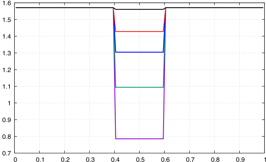
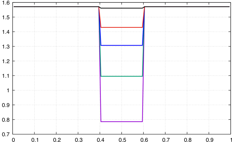
Figure 1: Comparison of flows at $t=0.0,\ 0.07,\ 0.14,\ 0.21,\ 0.5$: The vertical axis represents the Euler angle $\theta$ of the flow. The left side is computed by our scheme, and the right side is computed by using explicit form in Giga2015 .

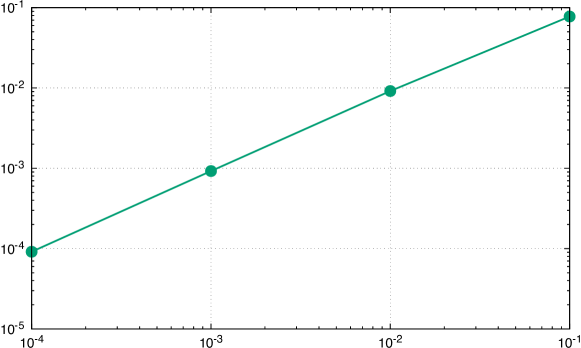
Figure 2: The $L^{2}$-error between our numerical scheme and the result in Giga2015 at $t=0.2$ with respect to the step size $\tau$.

5.2 Numerical example (2): $M=SO(3)$

5.2.1 The tangent spaces, orthogonal projections and exponential maps of $SO(3)$

Let $M(3)$ denote the linear space of all three-by-three matrices. $SO(3)$ denotes the group of rotations, i.e.,

$$SO(3):=\{x\in M(3)\mid x^{\top}x=xx^{\top}=I_{3},\ \det x=1\},$$

where $I_{3}$ denotes the identity matrix. Then $SO(3)$ is regarded as a matrix Lie group in $M(3)$. The set of all three-dimensional skew-symmetric matrices give the associated Lie algebra to $SO(3)$:

$$so(3):=\{X\in M(3)\mid X^{\top}=-X\}.$$

According to the general theory of Lie groups, $so(3)$ can be regarded as the tangent space $T_{I_{3}}(SO(3))$ at the identity, so that

$$so_{x}(3):=T_{x}(SO(3))=\{xX\mid X\in so(3)\}.$$

We equip $M(3)$ with the inner product

$$(X,Y):=\operatorname{trace}(X^{\top}Y)\quad\text{for}\quad X,Y\in M(3).$$

Then it induces a Riemannian metric on the submanifold $SO(3)$, which is invariant by the left- and right-translation of $SO(3)$. The exponential map $\exp_{e}$ with respect to a bi-invariant Riemannian metric at the identity of a compact Lie group is given by the exponential map of a Lie algebra ((He, , Ch. I​V, Theorem 3.3)) or equivalently, that of a matrix, hence

$$\exp_{e}(X)=\exp(X)\quad\text{for}\quad X\in T_{e}SO(3)\simeq so(3),$$

where $e=I_{3}$ in this matrix group. Since the induced Riemannian metric is left-invariant, the exponential map at $x\in SO(3)$ is of the form

$$\exp_{x}(X) =L_{x}\exp_{x}(x^{-1}X)$$

$$=L_{x}\exp(x^{\top}X)$$

for $X\in T_{x}\left(SO(3)\right)\simeq so_{x}(3)$, where $L_{x}$ denotes the left translation of $SO(3)$ given by $g\mapsto xg$. In other words, the exponential map is given in the following simple form

$$\exp_{x}(X)=x\exp(x^{\top}X),\quad X\in so_{x}(3).$$

Since the decomposition

$$M(3)=so_{x}(3)+\left\{xY\bigm{|}Y^{\top}=Y\right\},$$

$$X\mapsto\frac{X-xX^{\top}x}{2}+\frac{X+xX^{\top}x}{2}$$

is a direct orthogonal decomposition of $M(3)$, for arbitrarily fixed $x\in SO(3)$, the orthogonal projection $\pi_{x}\colon M(3)\to so_{x}(3)$ is given by

$$\pi_{x}(X):=\frac{X-xX^{\top}x}{2},\quad X\in M(3).$$ (5.5)

5.2.2 Euler angle

Rotations in $\mathbb{R}^{3}$ have nine components. The Euler angle (or Euler axis) representations are instrumental in reducing parameters of rotations. Given $R:=(R_{i,j})_{i,j=1}^{3}\in SO(3)$, its Euler angle (or Euler axis) representation is given by Rodrigues’ rotation formula

$$R=\cos\theta I_{3}+(1-\cos\theta)ee^{\top}+\sin\theta[e]_{x},$$ (5.6)

where $\theta\in[0,2\pi)$ and $e:=(e_{1},e_{2},e_{3})\in S^{2}$ denote the Euler angle and Euler axis of $R$, respectively, and $[e]_{x}$ is the cross product matrix of $e$. The following formulae give them:

$$\theta=\arccos{\left(\frac{R_{1,1}+R_{2,2}+R_{3,3}-1}{2}\right)},$$ (5.7)

$$(e_{1},e_{2},e_{3}):=\left(\frac{R_{3,2}-R_{2,3}}{2\sin\theta},\quad\frac{R_{1,3}-R_{3,1}}{2\sin\theta},\quad\frac{R_{2,1}-R_{1,2}}{2\sin\theta}\right),$$ (5.8)

and

$$[e]_{x}=\left(\begin{array}[]{ccc}0&-e_{3}&e_{2}\\ e_{3}&0&-e_{1}\\ -e_{2}&e_{1}&0\end{array}\right).$$

Since the Euler axis $e$ is in $S^{2}$, $e$ is represented by the spherical Euler angles $(\phi,\psi)\in[0,\pi)\times[0,2\pi)$. Therefore, $R$ is represented by three parameters $(\theta,\phi,\psi)\in[0,2\pi)\times[0,\pi)\times[0,2\pi)$.

5.2.3 Setup and numerical results

We use the following initial data $u_{0}$ with the Euler angles $\theta,\phi,\psi:\Omega=(0,1)\times(0,1)\to\mathbb{R}$:

$$\theta:=\sum_{i,j=0}^{2}\bm{\theta}_{i,j}\mathbf{1}_{I_{i}\times J_{j}},\quad\phi:=\sum_{i,j=0}^{2}\bm{\phi}_{i,j}\mathbf{1}_{I_{i}\times J_{j}},\quad\psi:=\sum_{i,j=0}^{2}\bm{\psi}_{i,j}\mathbf{1}_{I_{i}\times J_{j}},$$ (5.9)

where

$$\bm{\theta}=\left(\begin{array}[]{ccc}0.35\pi&0.2\pi&0.55\pi\\ 0.81\pi&0.64\pi&0.4\pi\\ 0.1\pi&0.7\pi&0.3\pi\end{array}\right),\quad\bm{\phi}=\left(\begin{array}[]{ccc}0.4\pi&0.5\pi&0.7\pi\\ 0.5\pi&0.3\pi&0.4\pi\\ 0.6\pi&0.3\pi&0.4\pi\end{array}\right),$$

$$\quad\bm{\psi}=\left(\begin{array}[]{ccc}0.2\pi&0.25\pi&0.3\pi\\ 0.25\pi&0.225\pi&0.2\pi\\ 0.3\pi&0.2\pi&0.35\pi\end{array}\right),$$

and

$$I_{0}=\left(0,\frac{2}{5}\right),\quad I_{1}=\left(\frac{2}{5},\frac{3}{5}\right),\quad I_{2}=\left(\frac{3}{5},1\right),$$

$$J_{0}=\left(0,\frac{1}{5}\right),\quad J_{1}=\left(\frac{1}{5},\frac{4}{5}\right),\quad J_{2}=\left(\frac{4}{5},1\right).$$

Figures 3 and 4 depict the results of numerical experiments under the above setting at times $t=0.0,0.05,0.1,0.25$ and $t=0.0,0.5,0.75,1.0$, respectively, where $\Omega$ is divided as $\bigcup_{i=1}^{N_{x}}\bigcup_{j=1}^{N_{y}}\Omega_{i,j}$, $\Omega_{i,j}:=((i-1)\Delta x,i\Delta x)\times((j-1)\Delta y,j\Delta y)$, in which we have defined both of $N_{x}$ and $N_{y}$ as $25$ and $\Delta x=1/N_{x}$ and $\Delta y=1/N_{y}$. Although no benchmark test for $SO(3)$-valued TV flow is known, we can see that our proposed numerical scheme works well since the facet-preserving property is satisfied, and the numerical solution finally reaches the constant solution.

Appendix A About the constant $C_{M}$

In this section, we derive a bound of the constant $C_{M}$ defined in (2.2). We recall several notations developed in computational geometry. A point $x\in\mathbb{R}^{\ell}$ is said to have the unique nearest point if there exists a unique point $p(x)\in M$ such that $p(x)\in\mathop{\mathrm{arg~{}min}}\limits_{p\in M}\left\|x-p\right\|_{\mathbb{R}^{\ell}}$. Let $S_{0}(M)$ denote the set of all points in $\mathbb{R}^{\ell}$ which do not have the unique nearest point. The closure $S(M)$ of $S_{0}(M)$ is called the medial axis of ${M}$. The local feature size $\mathrm{lfs}(M)$ of ${M}$ is the quantity defined by

$$\mathrm{lfs}({M}):=\inf_{p\in{M}}\inf_{q\in S_{0}(M)}\left\|p-q\right\|_{\mathbb{R}^{\ell}}.$$

Now, we assume that $M$ is compact. Then, $\mathrm{lfs}({M})$ is positive because $M$ has positive reach (Foote1984 ). We use the quantity $\mathrm{lfs}(M)$ to obtain that

$$\left\|p-q\right\|_{\mathbb{R}^{\ell}}\leq\mathrm{Dist}_{{M}}(p,q)\leq 2\max\left\{1,\frac{\mathrm{Diam}({M})}{\mathrm{lfs}({M})}\right\}\left\|p-q\right\|_{\mathbb{R}^{\ell}}$$ (A.1)

for each point $p$ and $q$ in $M$. Here, $\mathrm{Dist}_{M}(p,q)$ denotes the geodesic distance between $p$ and $q$. On the other hand, assuming that $M$ is path-connected, we have

$$\|\pi^{\bot}_{p}(p-q)\|_{\mathbb{R}^{\ell}}\leq\frac{1}{2}\ \mathrm{Curv}(M)\ \mathrm{Dist}_{M}(p,q)^{2}$$ (A.2)

for all $p,q\in M$. Therefore, if $M$ is a path-connected and a compact submanifold of $\mathbb{R}^{\ell}$, then we combine the inequalities (A.2) and (A.1) to obtain

$$\left\|\pi^{\bot}_{p}(p-q)\right\|_{\mathbb{R}^{\ell}}\leq 2\ \mathrm{Curv}({{M}})\ \max\left\{1,\frac{\mathrm{Diam}({M})}{\mathrm{lfs}({M})}\right\}^{2}\left\|p-q\right\|_{\mathbb{R}^{\ell}}^{2}$$ (A.3)

for all $p,q\in M$. Hence, we have

$$C_{M}\leq 2\ \mathrm{Curv}({{M}})\ \max\left\{1,\frac{\mathrm{Diam}({M})}{\mathrm{lfs}({M})}\right\}^{2}.$$ (A.4)

Finally, we remark that the proofs of (A.1) and (A.2) are found in Taguchi2018 .

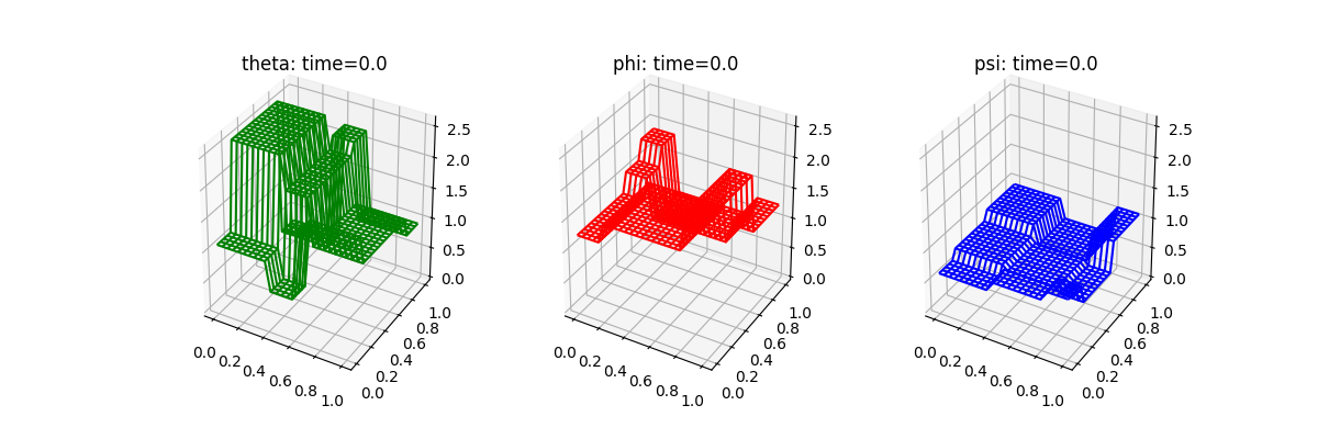
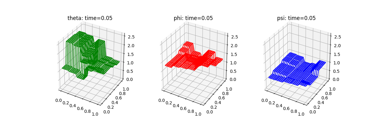
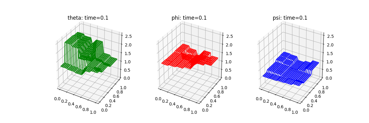
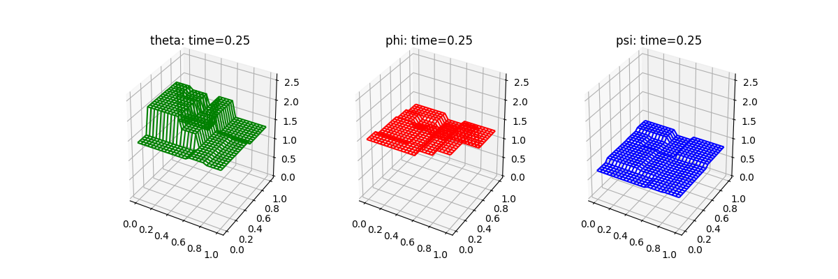
Figure 3: Numerical simulation of $SO(3)$-valued TV flow at $t=0.0,0.05,0.1,0.25$.

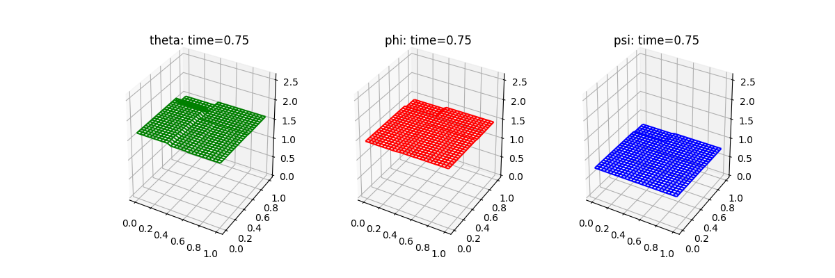
Figure 4: Numerical simulation of $SO(3)$-valued TV flow at $t=0.0,0.5,0.75,1.0$.

References

- (1) Absil, P.-A., Mahony, R., Sepulchre, R.: Optimization algorithms on matrix manifolds. xvi+224 pp., Princeton University Press, Princeton, NJ (2008)
- (2) Ambrosio, L., Gigli, N., Savare, G.: Gradient flows in metric spaces and in the space of probability measures. Lectures in Mathematics ETH Zürich, viii+333 pp., Birkhäuser Verlag, Basel (2005)
- (3) Barrett, J.W., Feng, X., Prohl, A.: On -harmonic map heat flows for and their finite element approximations. SIAM J. Math. Anal. 40, 1471–1498 (2008)
- (4) Basser, P.J., Mattiello, J., LeBihan, D.: MR diffusion tensor spectroscopy and imaging. Biophysics J. 66, 259–267 (1994)
- (5) Di Castroa, A., Giacomelli, L.: The 1-harmonic flow with values into a smooth planar curve. Nonlinear Anal. 143, 174–192 (2016)
- (6) Chefd’hotel, C., Tschumperlé, D., Deriche, R., Faugeras, O.: Constrained flows of matrix-valued functions: application to diffusion tensor regularization. Computer Vision-ECCV 2002, 251–265 (2002).
- (7) Chefd’hotel, C., Tschumperlé, D., Deriche, R., Faugeras, O.: Regularizing flows for constrained matrix-valued images. J. Math. Imaging Vision 20, 147–162 (2004).
- (8) Kovnatsky, A., Glashoff, K., Bronstein, M.M.: MADMM: A generic algorithm for non-smooth optimization on manifolds. Computer Vision-ECCV 2016, 680–696 (2016)
- (9) Christiansen, O., Lee, T.-M., Lie, J., Sinha, U., Chan, T.F.: Total variation regularization of matrix-valued images. International journal of biomedical imaging 2007, 11 pp. (2007)
- (10) Crandall, M.G., Liggett, T.M.: Generation of semi-groups of nonlinear transformations on general banach spaces. Amer. J. Math. 93, 265–298 (1971)
- (11) Feng, X., Yoon, M.: Finite element approximation of the gradient flow for a class of linear growth energies with applications to color image denoising. Int. J. Numer. Anal. Model. 6, 389–401 (2009)
- (12) Foote, R.L.: Regularity of the distance function. Proc. Amer. Math. Soc. 92, 1187–1220 (1984)
- (13) Giacomelli, L., Mazón, J.M., Moll, S.: The 1-harmonic flow with values into . SIAM J. Math. Anal. 45, 1723–1740 (2013)
- (14) Giacomelli, L., Mazón, J.M., Moll, S.: The 1-harmonic flow with values in a hyperoctant of the -sphere. Anal. PDE 7, 627–671 (2014)
- (15) Giacomelli, L., Łasica, M., Moll, S.: Regular 1-harmonic flow. arXiv:1711.07460, 24 pp. (2017)
- (16) Giga, M.-H., Giga, Y., Kobayashi, R.: Very singular diffusion equations, Proc. of the last Taniguchi Symposium (eds. Maruyama, M., Sunada, T.). Advanced Studies in Pure Math. 31, 93–125 (2001)
- (17) Giga, Y., Kobayashi, R.: On constrained equations with singular diffusivity. Methods Appl. Anal. 10, 253–278 (2003)
- (18) Giga, Y., Kuroda, H.: On breakdown of solutions of a constrained gradient system of total variation. Bol. Soc. Parana. Mat. 22, 9–20 (2004)
- (19) Giga, Y., Kuroda, H., Yamazaki, N.: An existence result for a discretized constrained gradient system of total variation flow in color image processing. Interdiscip. Inform. Sci. 11, 199–204 (2005)
- (20) Giga, Y., Kuroda, H., Yamazaki, N.: Global solvability of constrained singular diffusion equation associated with essential variation. Internat. Ser. Numer. Math. 154, 209–218 (2006)
- (21) Giga, Y., Kuroda, H.: A counterexample to finite time stopping property for one-harmonic map flow. Commun. Pure Appl. Anal. 14, 1–5 (2015)
- (22) Giga, Y., Ueda, Y.: Numerical computations of split Bregman method for fourth order total variation flow. J. Comput. Phys. 405, 190114 (2020)
- (23) Goldstein, T., Osher, S.: The split Bregman method for L1-regularized problems. SIAM J. Imaging Sci. 2, 323–343 (2009)
- (24) Helgason, S.: Differential geometry, Lie groups, and symmetric spaces. Pure and Applied Mathematics, 80. Academic Press, Inc. [Harcourt Brace Jovanovich, Publishers], New York-London, xv+628 pp. (1978)
- (25) Kobayashi, R., Warren, J.A.: Modeling the formation and dynamics of polycrystals in 3D. Phys. A 356, 127–132 (2005)
- (26) Kobayashi, R., Warren, J.A., Carter, W.C.: A continuum model of grain boundaries. Phys. D 140, 141–150 (2000)
- (27) Lai, R., Osher, S.J.: A splitting method for orthogonality constrained problems. J. Sci. Comput. 58, 431–449 (2014)
- (28) Łasica, M., Moll, S., Mucha, P. B.: Total variation denoising in anisotropy. SIAM J. Imaging Sci. 10, 1691–1723 (2017)
- (29) Li, G., Pong, T.K.: Global convergence of splitting methods for nonconvex composite optimization. SIAM J. Optim. 25, 2434–2460 (2015)
- (30) Oberman, A., Osher, S., Takei, R., Tsai, R.: Numerical methods for anisotropic mean curvature flow based on a discrete time variational formulation. Commun. Math. Sci. 9, 637–662 (2011)
- (31) Dal Passo, R., Giacomelli, L., Moll, S.: Rotationally symmetric 1-harmonic maps from to . Calc. Var. Partial Differential Equations 32, 533–554 (2010)
- (32) Pennec, X., Fillard, P., Ayache, N.: A Riemannian framework for tensor computing. International Journal of Computer Vision 66, 41–66 (2006)
- (33) Požár, N.: On the self-similar solutions of the crystalline mean curvature flow in three dimensions. arXiv:1806.02482, 28 pp. (2018)
- (34) Rulla, J.: Error analysis for implicit approximations to solutions to Cauchy problems. SIAM J. Numer. Anal. 33, 68–87 (1996)
- (35) Setzer, S.: Splitting methods in image processing, Ph.D thesis, Universitat Mannheim. 174 pp. (2009)
- (36) Taguchi, K.: On discrete one-harmonic map flows with values into an embedded manifold on a multi-dimensional domain. Adv. Math. Sci. Appl. 27, 81–113 (2018)
- (37) Tang, B., Sapiro, G., Caselles, V.: Color image enhancement via chromaticity diffusion. IEEE Transactions on Image Processing 10, 701–707 (2001)
- (38) Vese, L.A., Osher, S.J.: Numerical methods for -harmonic flows and applications to image processing. SIAM J. Numer. Anal. 40, 2085–2104 (2009)
- (39) Weinmann, A., Demaret, L., Storath, M.: Total variation regularization for manifold-valued data. SIAM J. Imaging Sci. 7, 2226–2257 (2014)
- (40) Wang, Y., Yin, W., Zeng, J.: Global convergence of ADMM in nonconvex nonsmooth optimization. J. Sci. Comput. 35 pp. (2018)
- (41) Zhang, J., Ma, S., Zhang, S.: Primal-Dual optimization algorithms over Riemannian manifolds: an iteration complexity analysis. arXiv:1710.0223, 44 pp. (2017)